Pipetting & eGels
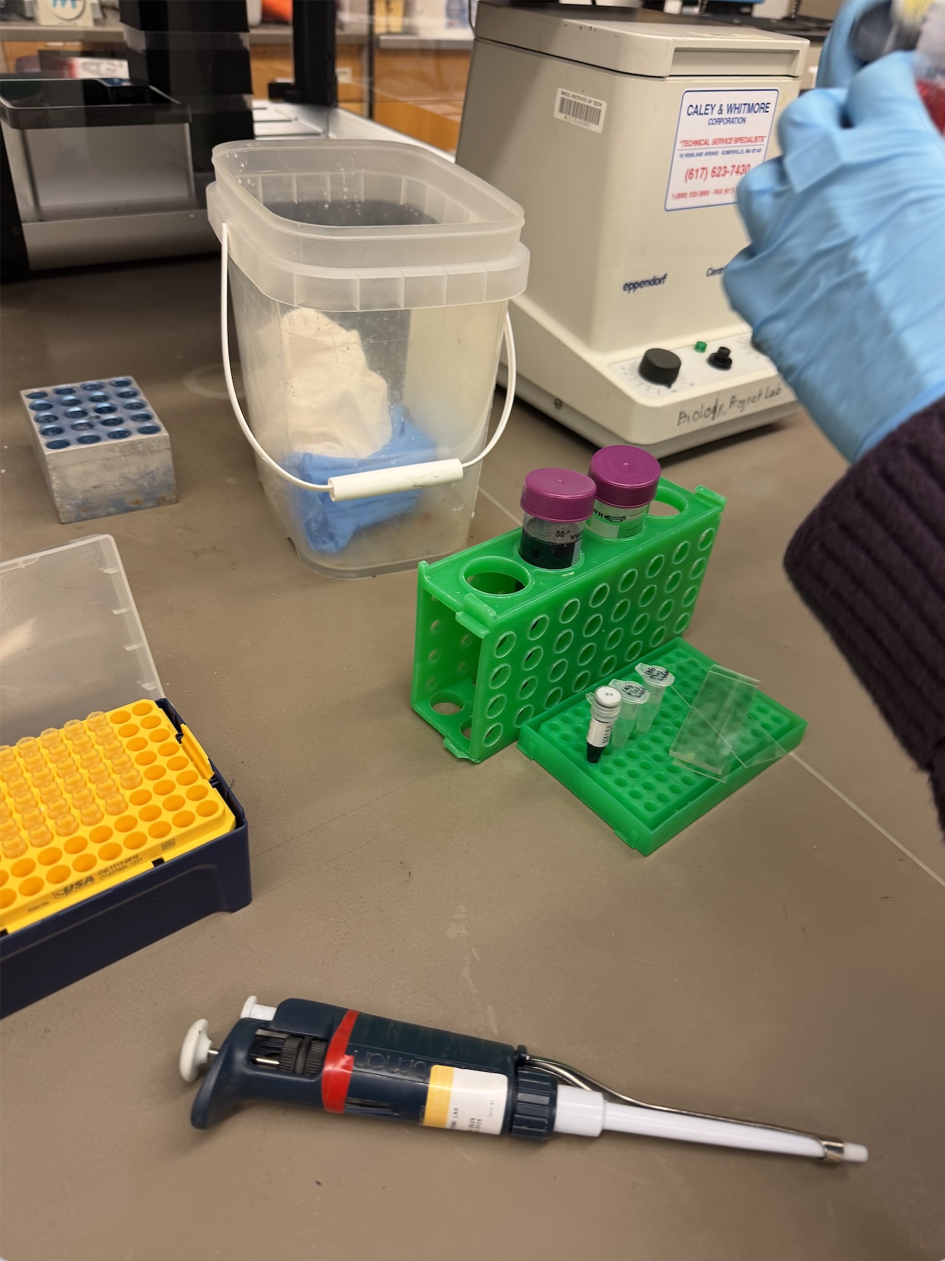
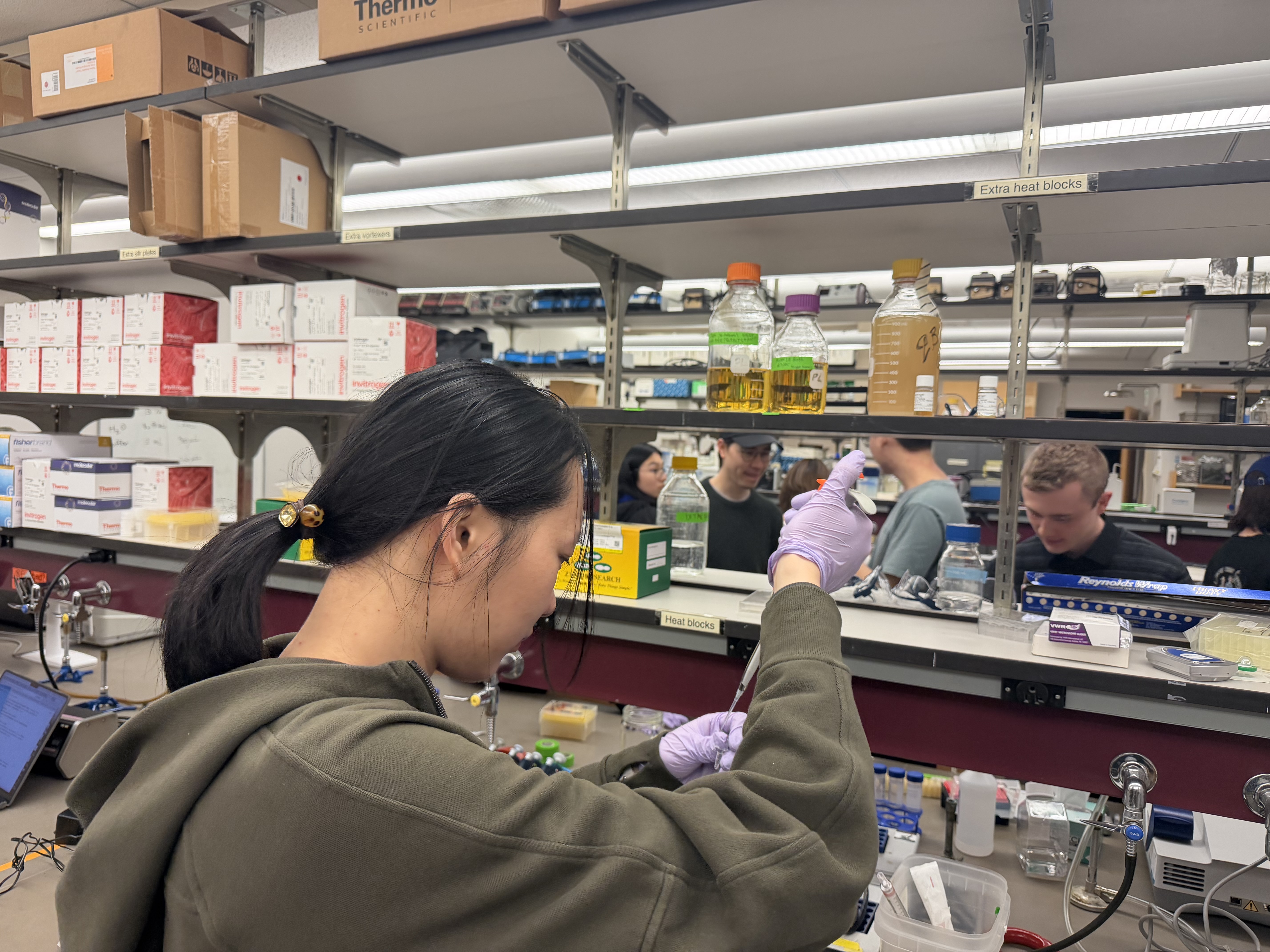
In this week’s lab, we were tasked with familiarizing ourselves with standard pipetting equipment. We utilized P20, P200, and P2000 micropipettes, along with petri dishes and glass slides. Having prior experience in a wet lab, it was fun to explore the equipment artistically.
I started by creating some “droplet art” on a glass slide using colored water.
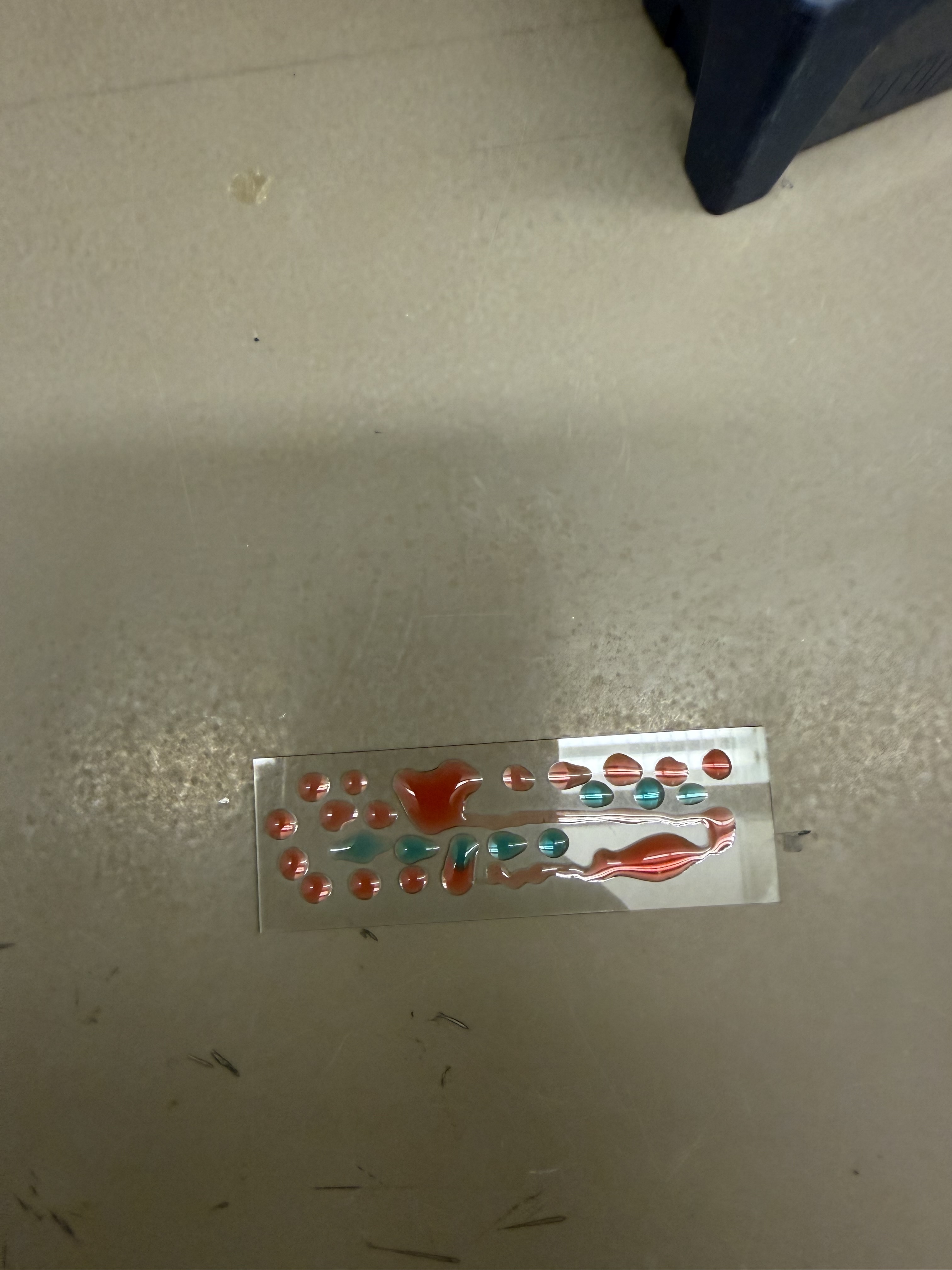
I then decided to make a smiley face and a DNA strand in the same fashion, pipetting individual droplets of colored water and “streaking” them to create lines.
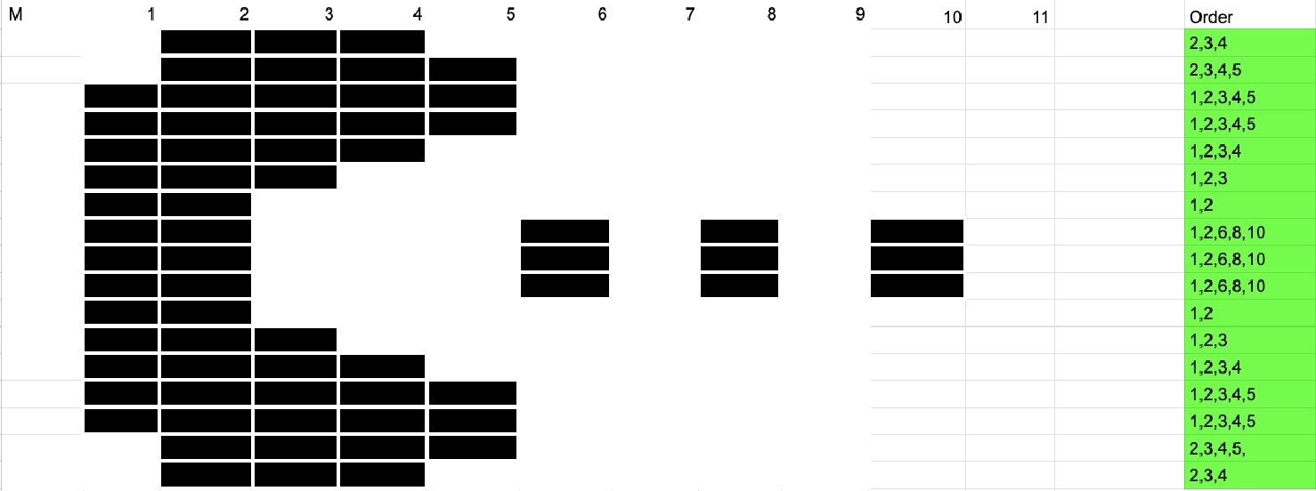
Lab: DNA Gel Art Today in lab, we attempted to make DNA Gel Art using restriction enzymes and software (Benchling). In recitation, we were given an example of someone using time-controlled gel work to create an image, so I came up with a plan to use that framework to create an image of Pac-Man.
I used SalI, which cuts only a single 500 bp strand from lambda DNA, for my digest to create my “blocks” that I would effectively “stack” as I pipetted them at interval times on the gel.
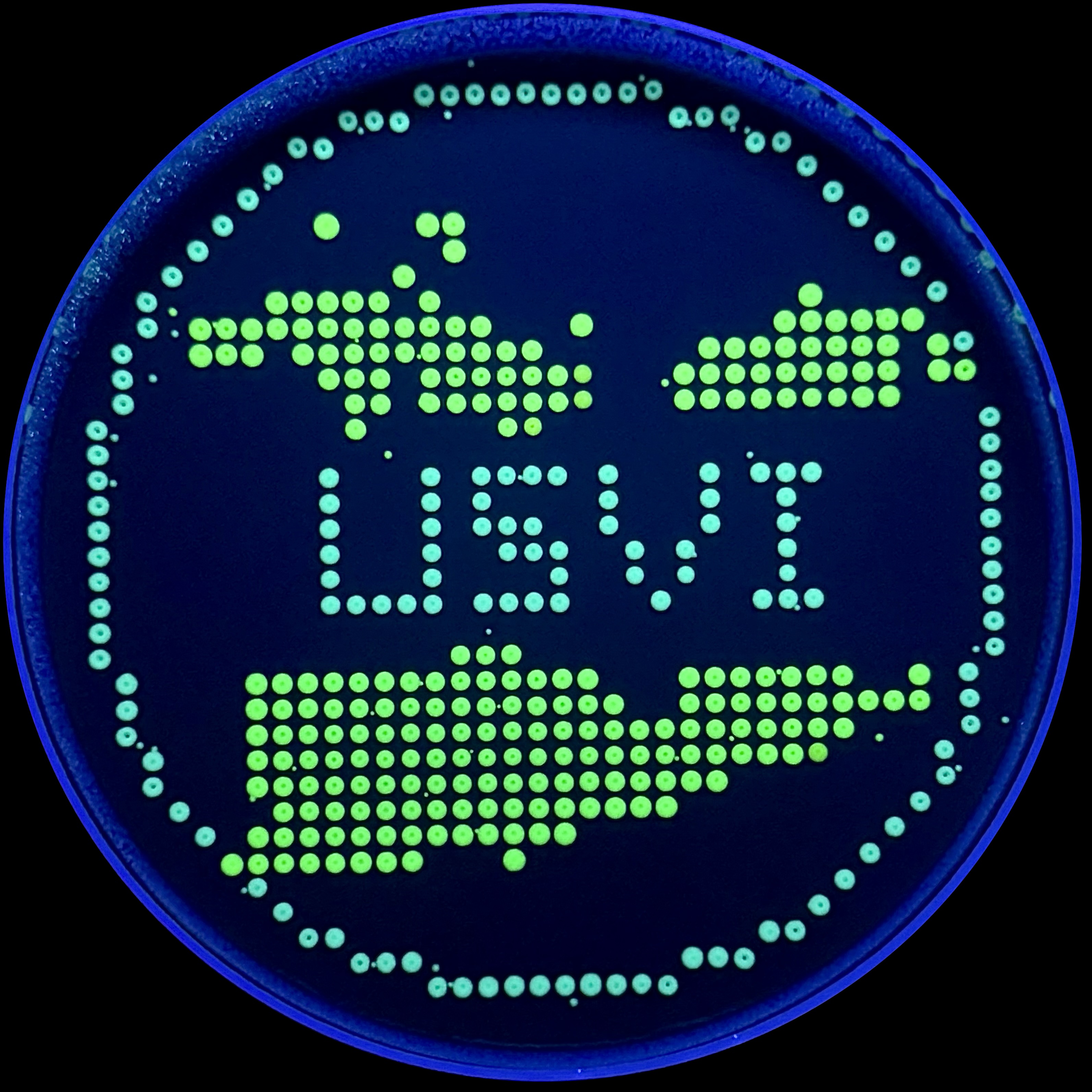
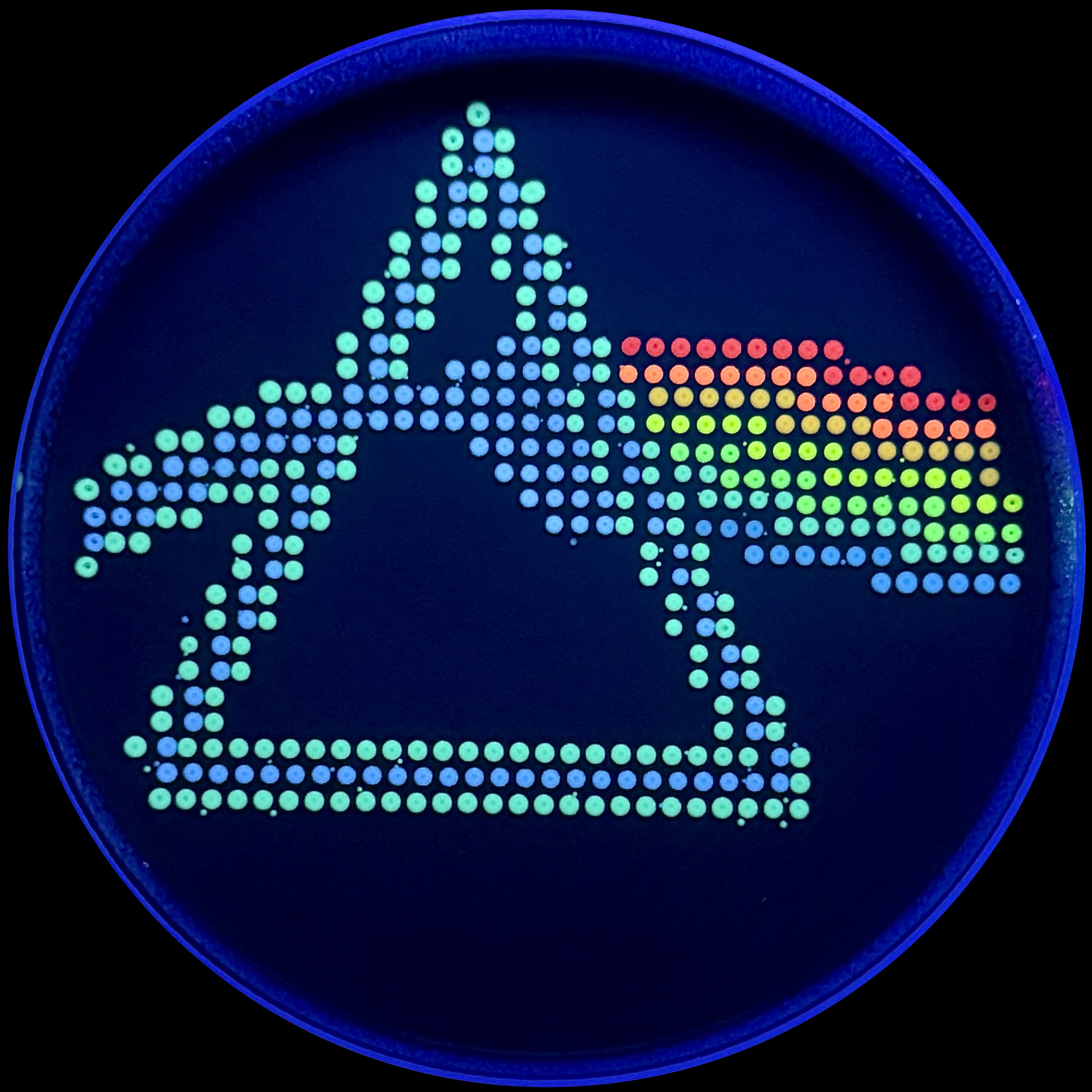
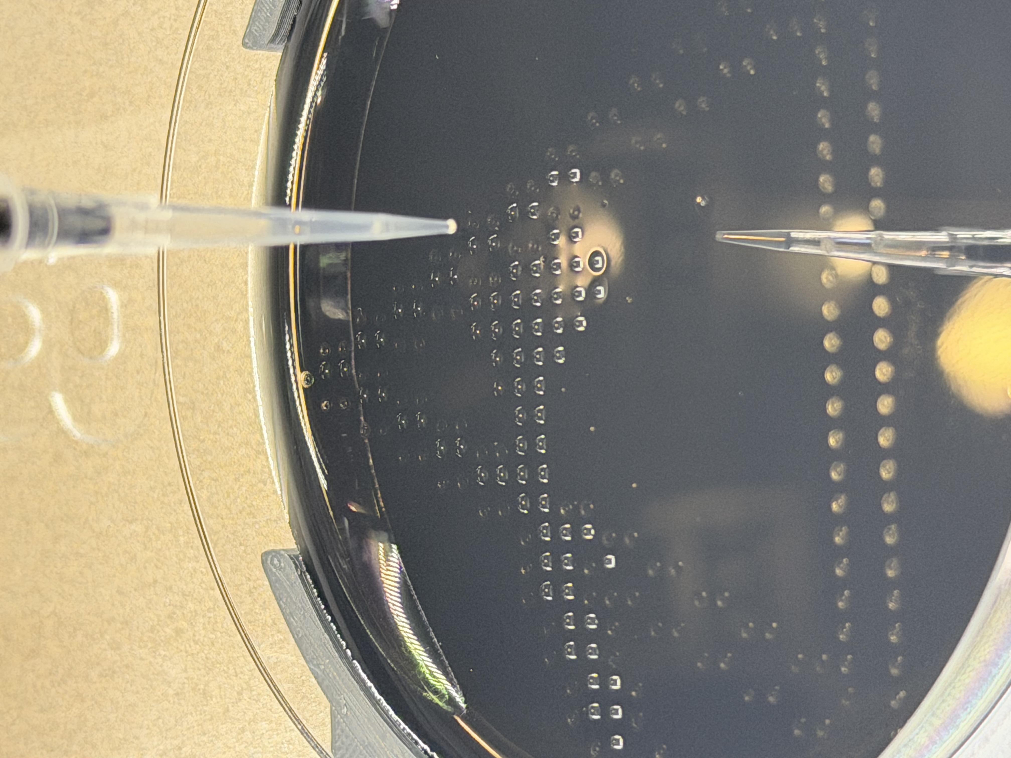
This week in lab, we used the Opentrons machine, giving us a taste of lab automation with an artistic twist. We pipetted flourescent, genetically engineered E.coli onto agar mixed with activated charcoal to create our design and canvas respectively. After a 16 hour incubation period, we were able to see images of our results under UV light! I decided to make two designs, one of the US Virgin Islands to pay homage to where I’m from, and the other was the Dark Side of the Moon Album Cover, as I thought it used a good variety of colors. The robot moved from top left to bottom right, which prompted a discussion with Ronan about the most optimal pathing system for the trajectory. The robot’s movement is controlled by a Python script, and Ronan created a website to generate the coordinates of each colored pixel, which the script implemented.
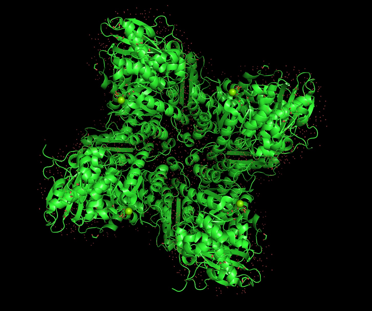
Protein Selection Briefly describe the protein you selected and why you selected it. Again, continuing with my idea for designing a carbon sequestration system, I am going to be looking at Rubisco, the most abundant protein on earth. Rubisco catalyzes photosynthesis in plants, converting atmospheric CO2 into an organic three-carbon acid that eventually is built up into sugars for plant growth. It is made of 8 large subunits and 8 small subunits.
Lab Option 1: L-Protein Mutational Analysis Experimental Validation & DMS This lab provides a Deep Mutational Scanning (DMS) style validation of the L-Protein. By cross-referencing experimental lysis results—where a score of 1 indicates functional lysis and 0 indicates non-functional—with the Log-Likelihood Ratio (LLR) Heatmap generated via ESM2, we can assess the predictive power of protein language models.
Day 1: Preparation of DNA Fragments Background In this two-day lab, we modified the color-generating chromophore of the purple Acropora millepora chromoprotein (amilCP) to create a variety of orange, pink, and blue mutants.
We performed two sets of Polymerase Chain Reactions (PCR) to prepare for a Gibson Assembly. The insert PCR region spans the 24 base pairs before the chromophore to just beyond the gene transcription terminator. The forward primer includes an intentional mismatch for site-directed mutagenesis of the mUAV DNA plasmid. These mutants were then expressed in chemically competent E. coli cells.
Intracellular Artificial Neural Networks (IANNs) In this two-day lab, we designed and built our very own IANN using a library of plasmids from the Ron Weiss lab and human embryonic kidney (HEK) 293 cells. IANNs differ from traditional synthetic genetic circuits because IANNs can perform analog computations, rather than being limited to digital computations. IANNs are also universal function approximators—given an adequate number of intracellular artificial neurons, you can use an IANN to achieve any input/output behavior you’d like.
Fungal Materials Follow-up The first thing we did was look at our mycelium molds (no pun intended). We are tracking the growth and structural integrity of the fungal networks as they colonize the substrates.
Protein Purification: An Introduction To isolate our protein of interest, we first had to grow the cells and then lyse them using a combination of B-PER (Bacterial Protein Extraction Reagent) and sonication. This process breaks open the cell membranes, resulting in a lysate solution (labeled as Tube A) that contains the total protein content of the cells.
Subsections of Labs
Week 1 Lab: Pipetting
Pipetting & eGels
In this week’s lab, we were tasked with familiarizing ourselves with standard pipetting equipment. We utilized P20, P200, and P2000 micropipettes, along with petri dishes and glass slides. Having prior experience in a wet lab, it was fun to explore the equipment artistically.
I started by creating some “droplet art” on a glass slide using colored water.
I then decided to make a smiley face and a DNA strand in the same fashion, pipetting individual droplets of colored water and “streaking” them to create lines.
I noticed another labmate using petri dishes for her art. Given the hydrophobic coating on the plate, the droplets formed more uniform spheres that maintained their geometry better than on the glass slides. I proceeded to create another drawing on the petri dish.
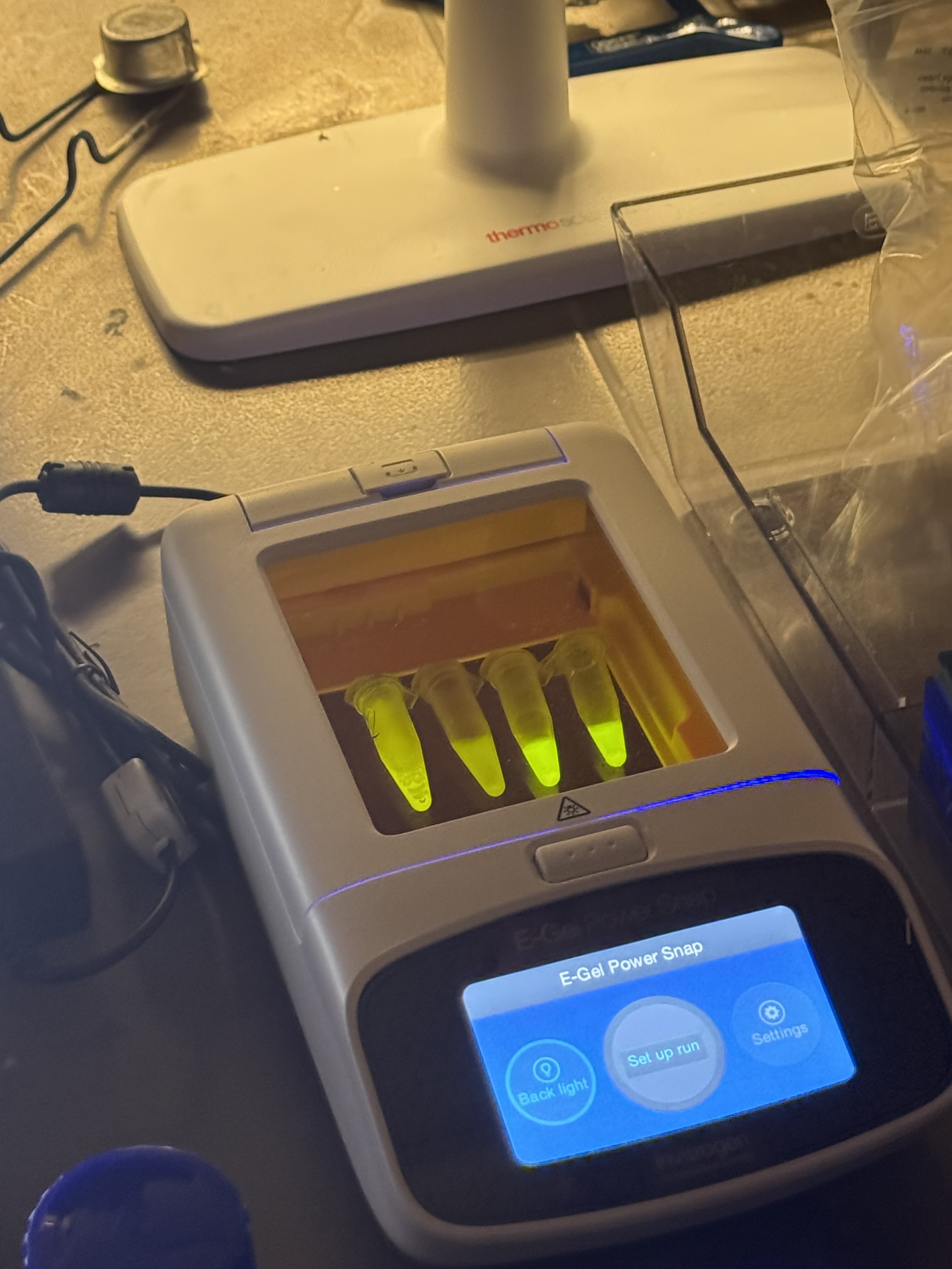
Finally, we used an eGel, a piece of technology I had never seen before. I was thoroughly impressed—no loading buffer, no separate imaging box, and no dye required. The process was incredibly streamlined. Another classmate and I alternated pipetting the provided ladder sample and dH2O into the lanes of the gel. The eGel even allows for mid-run imaging, which I was delighted to take advantage of.
The first lab has definitely made me excited to get my hands on the rest of the equipment we will use in this class, and it provided a nice artistic lens through which to view a simple task like pipetting. :)
Gemini AI was consulted for formatting
Week 2 Lab: DNA Gel Art
Lab: DNA Gel Art
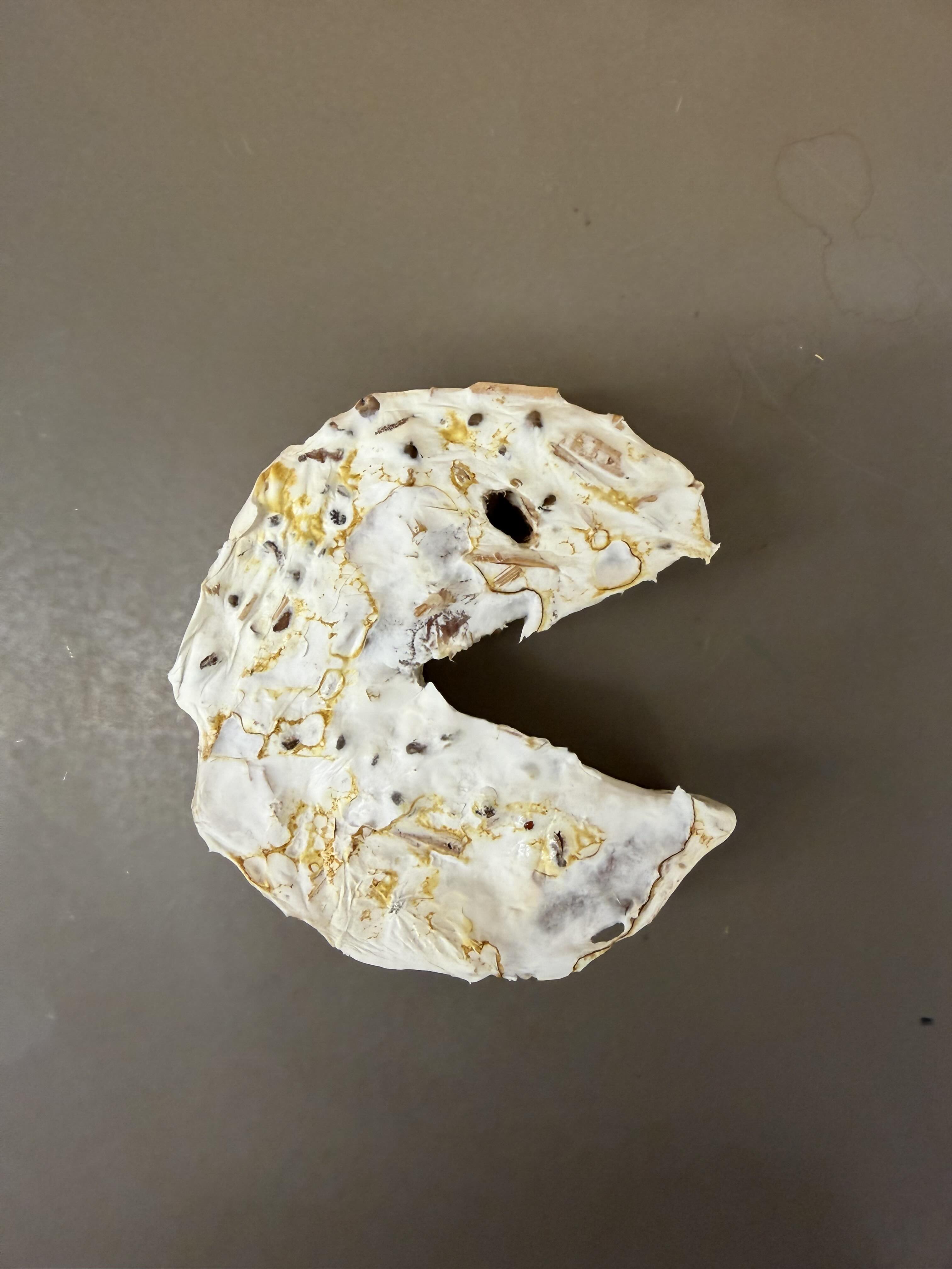
Today in lab, we attempted to make DNA Gel Art using restriction enzymes and software (Benchling). In recitation, we were given an example of someone using time-controlled gel work to create an image, so I came up with a plan to use that framework to create an image of Pac-Man.
I used SalI, which cuts only a single 500 bp strand from lambda DNA, for my digest to create my “blocks” that I would effectively “stack” as I pipetted them at interval times on the gel.
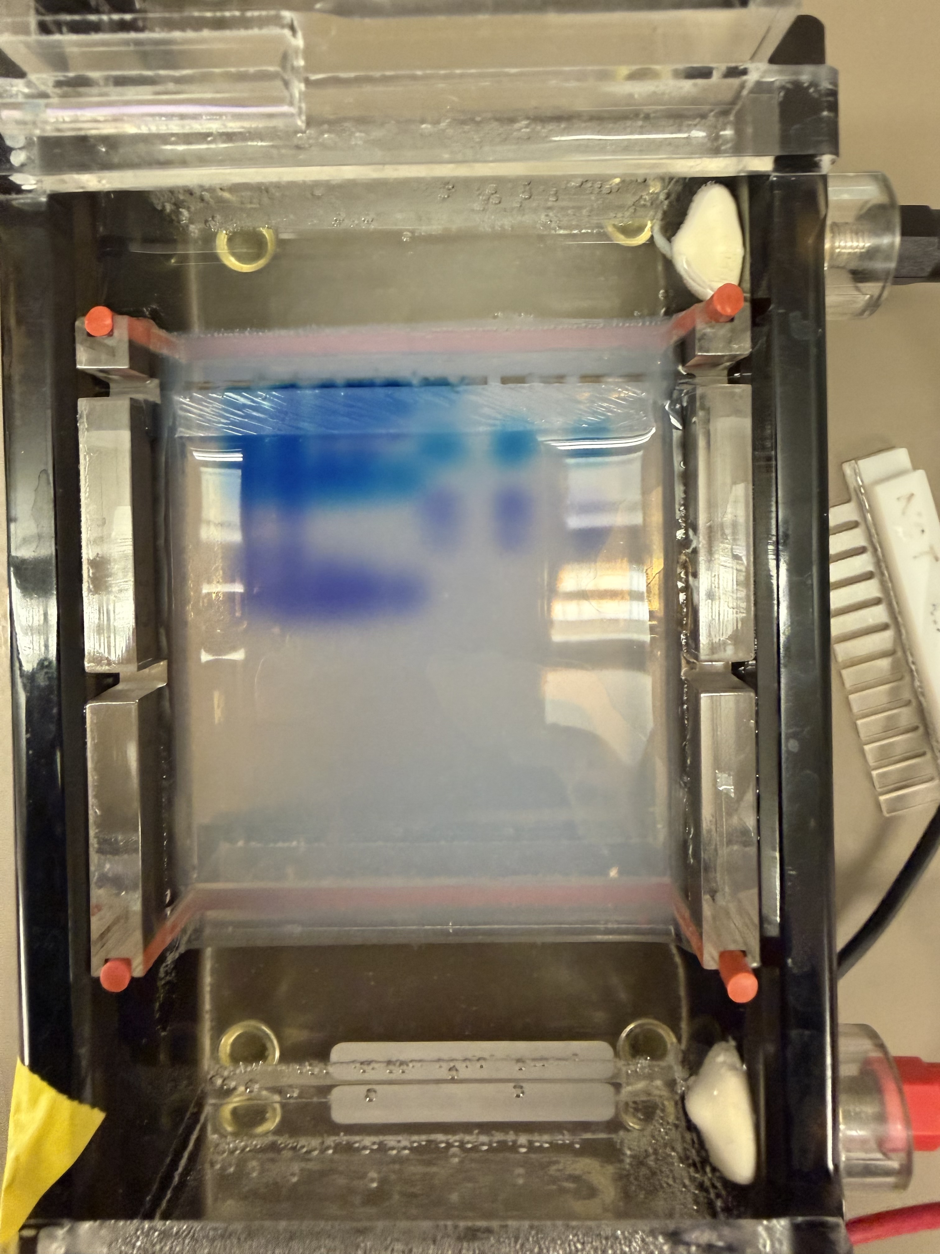
I worked with another classmate, Devorah, and together we created our gel with the agar and TAE buffer, and ran our gels at 150+ volts.
Devorah tried to make a dragonfly-looking structure, which required a variety of restriction enzymes. After making our gel, we let our digest reactions incubate for 30 minutes, then created the loading samples and ran the gels. I set serial, 4-minute timers that prompted me to pipette the next “row” to create my pacman image.
After I was finished, my gel took an unfortunate tumble to the ground, and was imaged in pieces.
In the end, it looks like the digestion did not go according to plan, as no DNA appeared to have traveled down the gel, and only the dye created the facade image. However, It is also entirely possible that by serially pipetting into the same wells, a buildup of DNA occurred and the 500bp strands that were supposed to fall into place got stuck (I am less inclined to believe this, though, because I would expect at least 1 500bp band to make it to the bottom, and none were present effectively). Overall, this was a fun project, and I took pleasure in trying to come up with an alternative approach to execute my creative goal, eventhough my results didn’t come out as expected.
Devorah’s design also wasn’t quite what we were expecting, and I think its also related to an improper digestion reaction.
Gemini AI was consulted for formatting
Week 3 Lab: Opentrons
This week in lab, we used the Opentrons machine, giving us a taste of lab automation with an artistic twist. We pipetted flourescent, genetically engineered E.coli onto agar mixed with activated charcoal to create our design and canvas respectively. After a 16 hour incubation period, we were able to see images of our results under UV light! I decided to make two designs, one of the US Virgin Islands to pay homage to where I’m from, and the other was the Dark Side of the Moon Album Cover, as I thought it used a good variety of colors. The robot moved from top left to bottom right, which prompted a discussion with Ronan about the most optimal pathing system for the trajectory. The robot’s movement is controlled by a Python script, and Ronan created a website to generate the coordinates of each colored pixel, which the script implemented.
Week 4 Lab: Protein Design Part I
Protein Selection
Briefly describe the protein you selected and why you selected it.
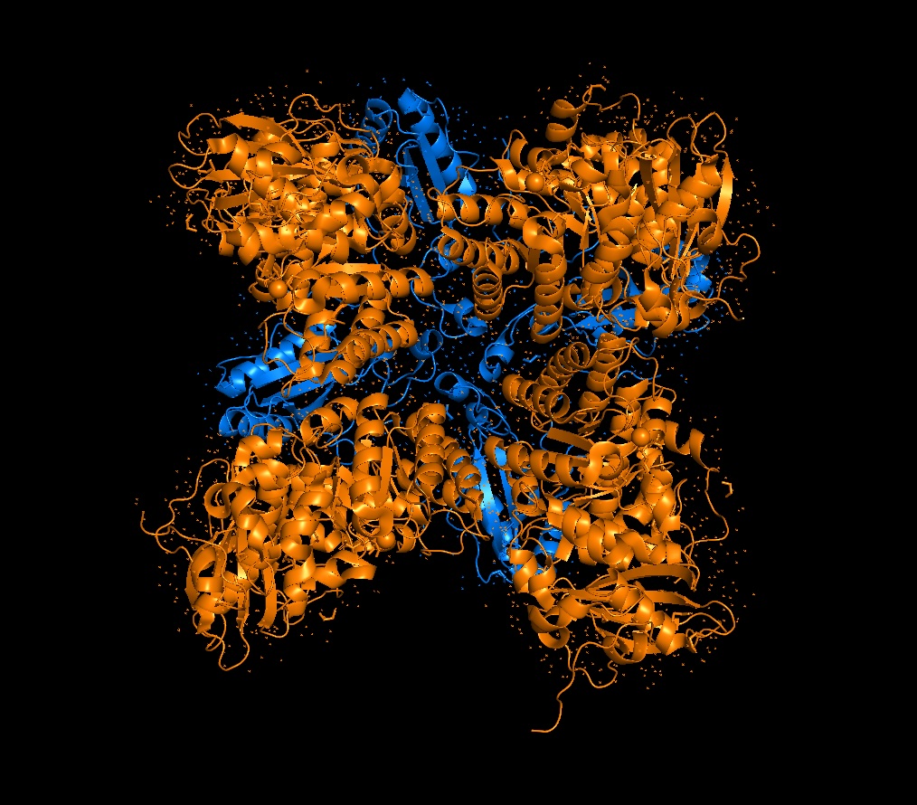
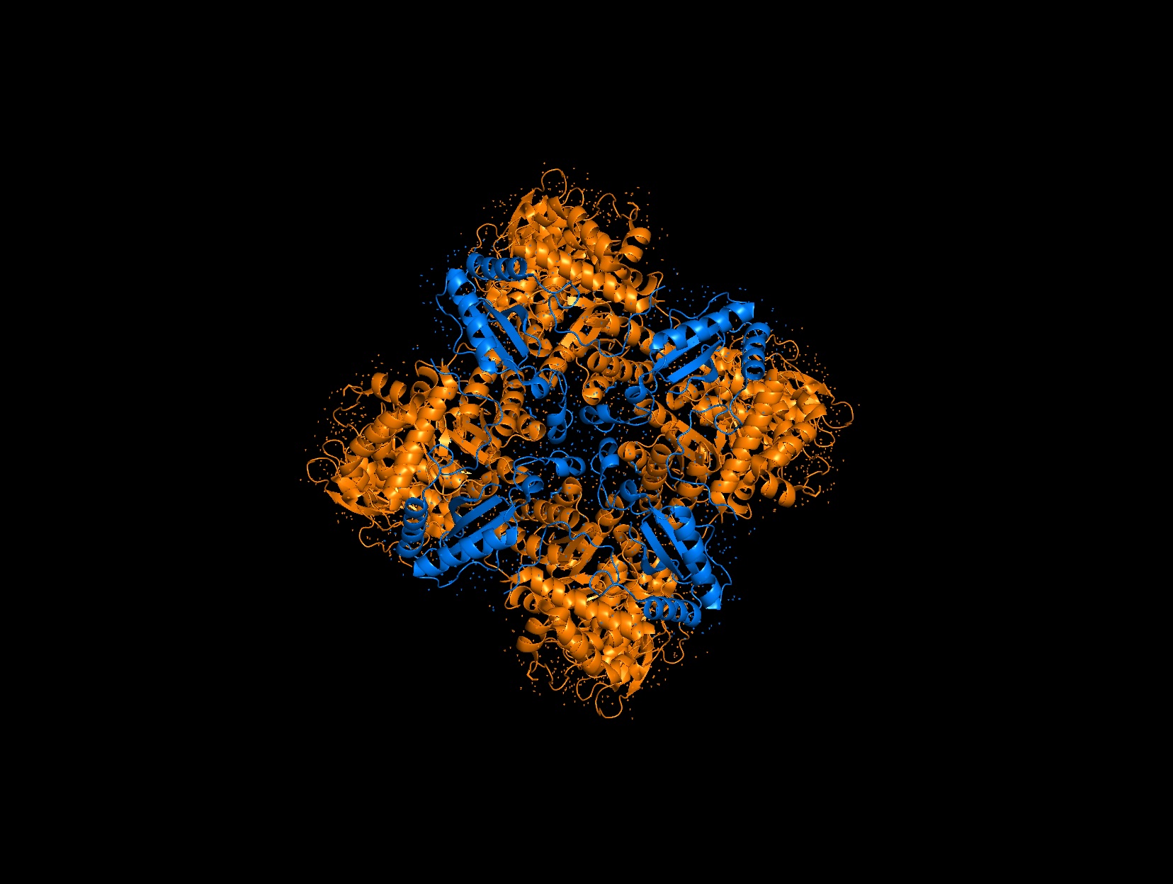
Again, continuing with my idea for designing a carbon sequestration system, I am going to be looking at Rubisco, the most abundant protein on earth. Rubisco catalyzes photosynthesis in plants, converting atmospheric CO2 into an organic three-carbon acid that eventually is built up into sugars for plant growth. It is made of 8 large subunits and 8 small subunits.
How long is it? What is the most frequent amino acid?
The Large Subunit is roughly 475 amino acids long and the small subunit is roughly 175 amino acids long. The most frequent amino acid is Alanine (A) in both subunits with ~13 A’s in the small chain and ~46 in the large chain.
Homologs and Structure
How many protein sequence homologs are there for your protein?
There are 8 versions of Rubisco Large and Small subunits that are marginally different and assemble together to create a 16-mer (hexadecamer) protein.
Does your protein belong to any protein family?
They belong to the Rubisco Large and Small subunit chain families.
When was the structure solved? Is it a good quality structure?
Form I, the 8L, 8S hexadecamer was solved in the 1990s with an initial resolution of 2.2 angstroms, with specific structures like that of Chlamydomonas reinhardtii being solved for 1.4 angstroms in 2001. This is a very good quality structure (smaller resolution is better, typically < 2.70 Å).
Are there any other molecules in the solved structure apart from protein?
Yes, magnesium ions and carbamylated lysine.
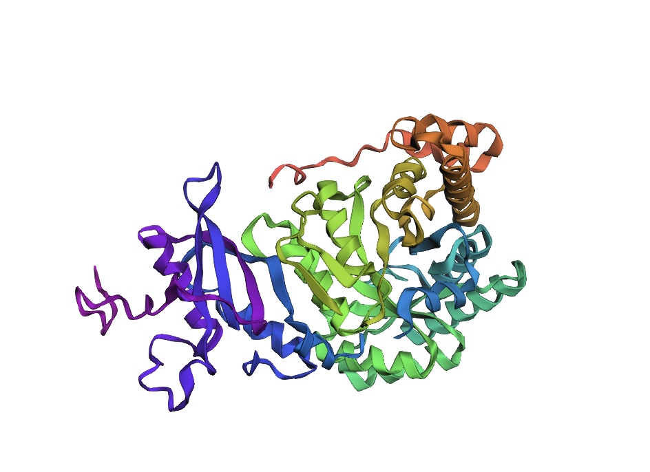
3D Molecule Visualization (PyMol)
Visualize the protein as “cartoon”, “ribbon” and “ball and stick”.
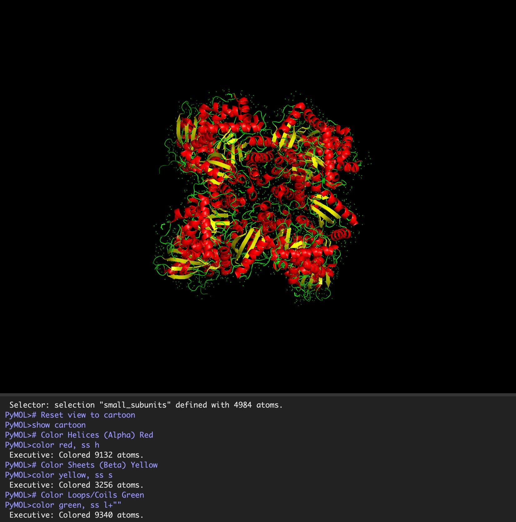
Color the protein by secondary structure. Does it have more helices or sheets?
It has roughly 40% helices and 20% beta sheets.
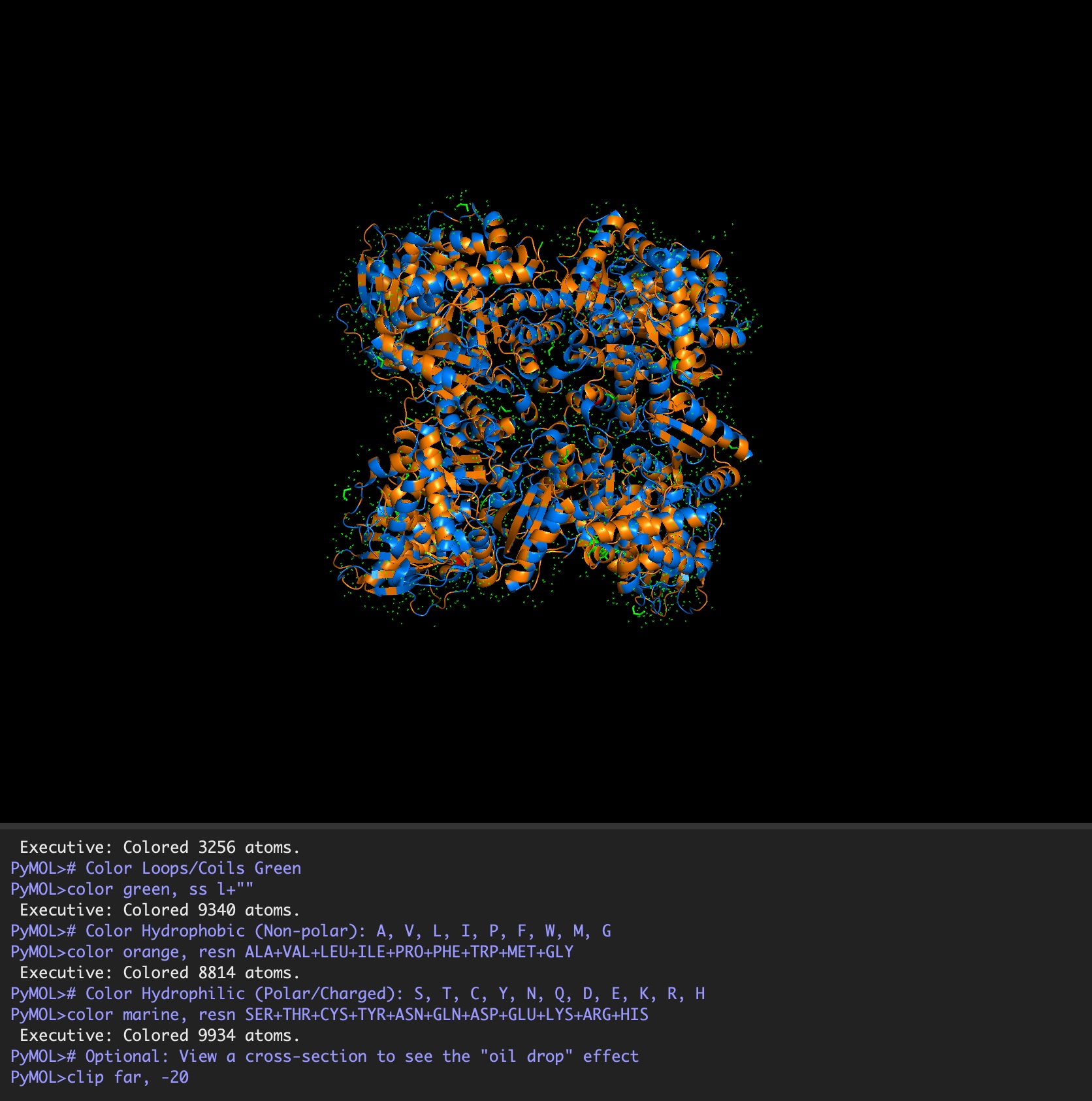
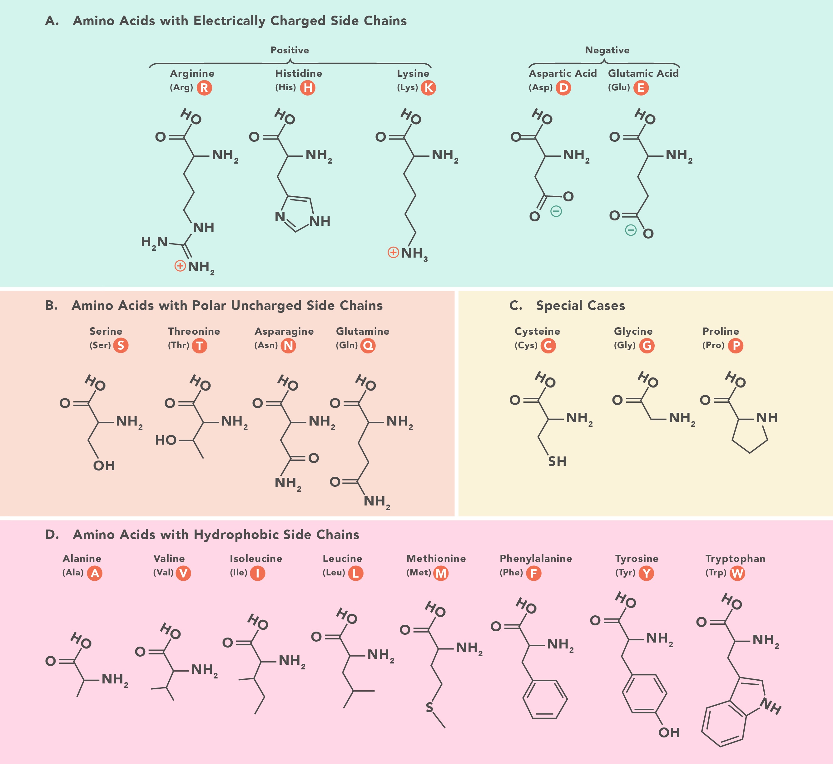
Color the protein by residue type. What can you tell about the distribution of hydrophobic vs hydrophilic residues?
It is a mosaic of hydrophobic and hydrophilic residues, making it efficient in aqueous environments but also able to interact with hydrophobic residues.
Visualize the surface of the protein. Does it have any “holes” (aka binding pockets)?
Because the holoenzyme is made of 8 large subunits, it has 8 identical active sites. The active pocket sites contain deep indentations located at the mouth of each TIM barrel. This is where Ribulose-1,5-bisphosphate and CO2 meet to be converted into sugar.
The central pore is visible from the “top” (along its axis of symmetry) and is a prominent hole/channel running through the center of the entire L8S8 complex. There are also smaller crevices between the small subunits and the large subunit core, which some researchers believe might play a role in gas or metabolite diffusion. Deep into those 8 pockets is where the magnesium ions are located, which coordinate the substrates and are necessary for the reaction to proceed.
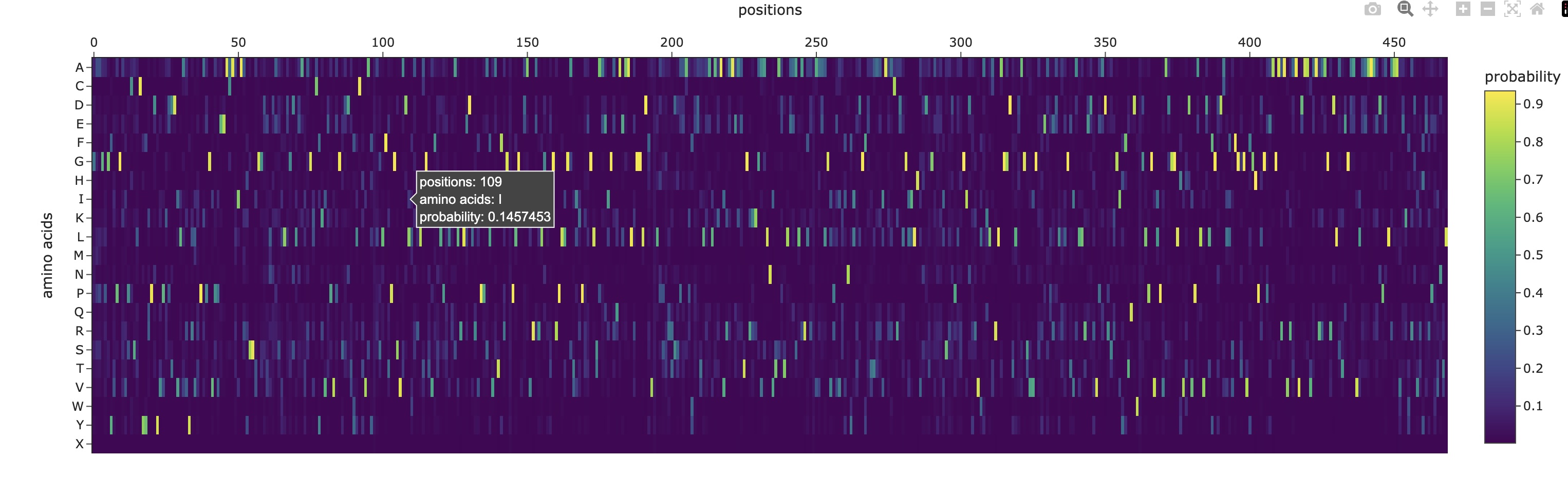
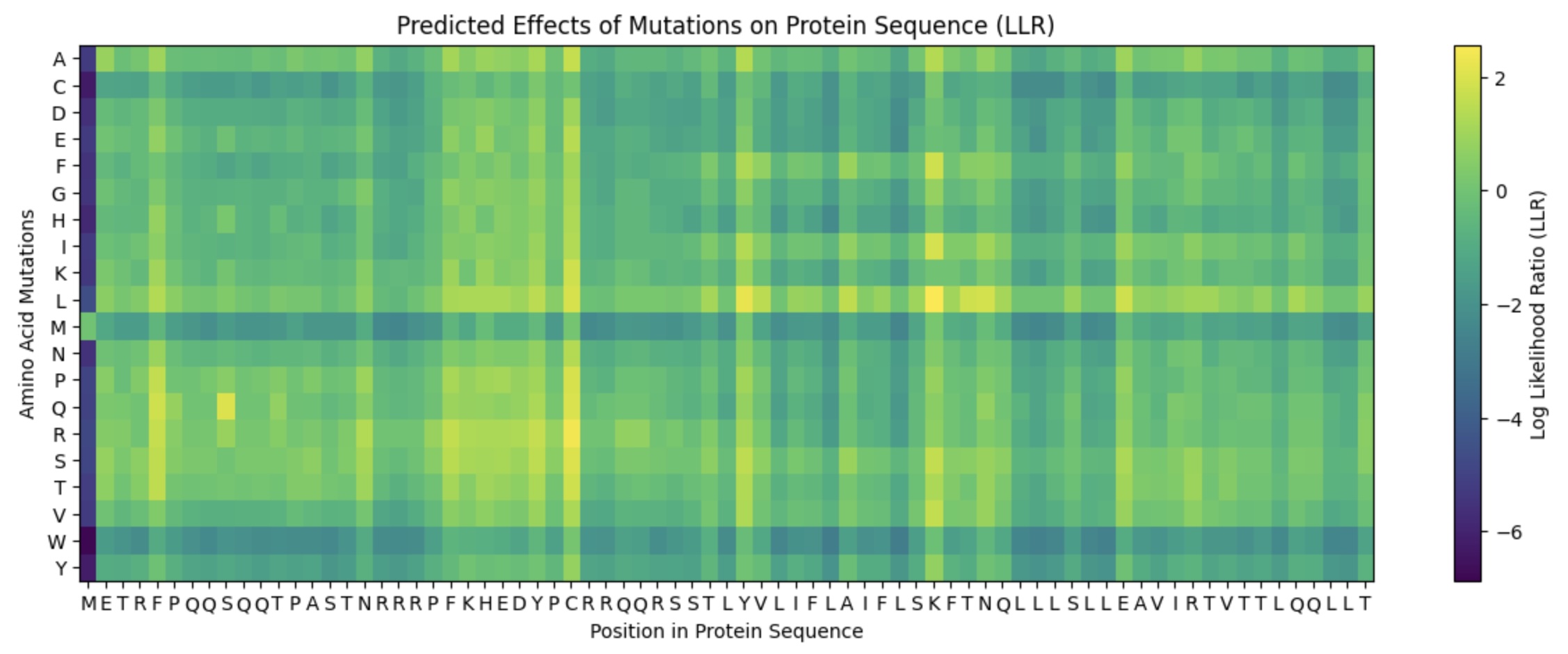
Deep Mutational Scans
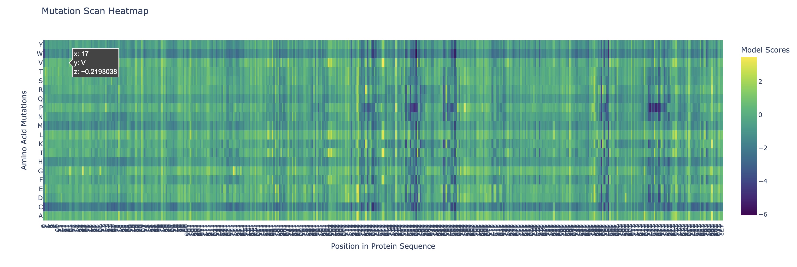
Use ESM2 to generate an unsupervised deep mutational scan of your protein based on language model likelihoods.
Can you explain any particular pattern? (choose a residue and a mutation that stands out)
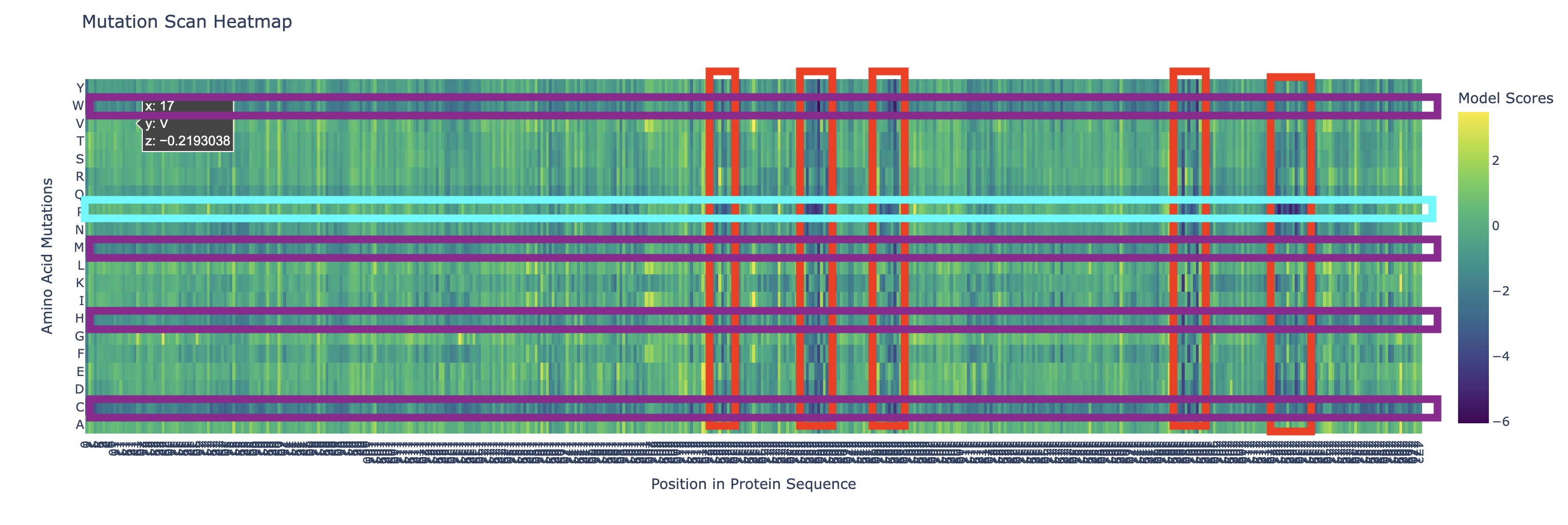
There are a couple of trends I’ve noticed from this mutational scan. There seem to be 5 main evolutionarily conserved sequences that result in catastrophic damage to the protein if substituted (these are the vertical lines I’ve highlighted in red). Additionally, there are many faintly dark vertical bands, indicating that Rubisco is generally highly conserved which I think is strongly supported by the fact that it’s the most abundant protein on earth (the sequence works and thus has resisted change over a long time scale).
Additionally, there are a couple main horizontal bands of negative change, mainly in amino acids W, C, M, H, Q (outlined in purple). This is actually not that surprising in my opinion. Methionine (M) and Cysteine (C) are unique in that they are the only two that contain sulfur atoms which could cause negative effects in a multitude of ways (sulfur is huge so steric hindrance is likely, it’s very polarizable so it makes an excellent nucleophile with higher reactivity, and its redox affinity allows for structural organizations like disulfide bridges to occur). Tryptophan (W) is a gigantic amino acid with its aromatic ring that again causes a lot of conformational changes due to sterics. Histidine (H) is one of three positively charged amino acid residues and altering electrostatic character (acidity/basicity) usually has significant effects. And Glutamine (Q) is a polar amino acid, again introducing a tangible change to binding character.
What I found interesting was that a substitution of Proline (P) (teal) across the protein was predicted to increase efficiency except at the highly conserved regions I highlighted earlier, where a substitution to proline was significantly more negatively impactful than other amino acids which I found a bit strange.
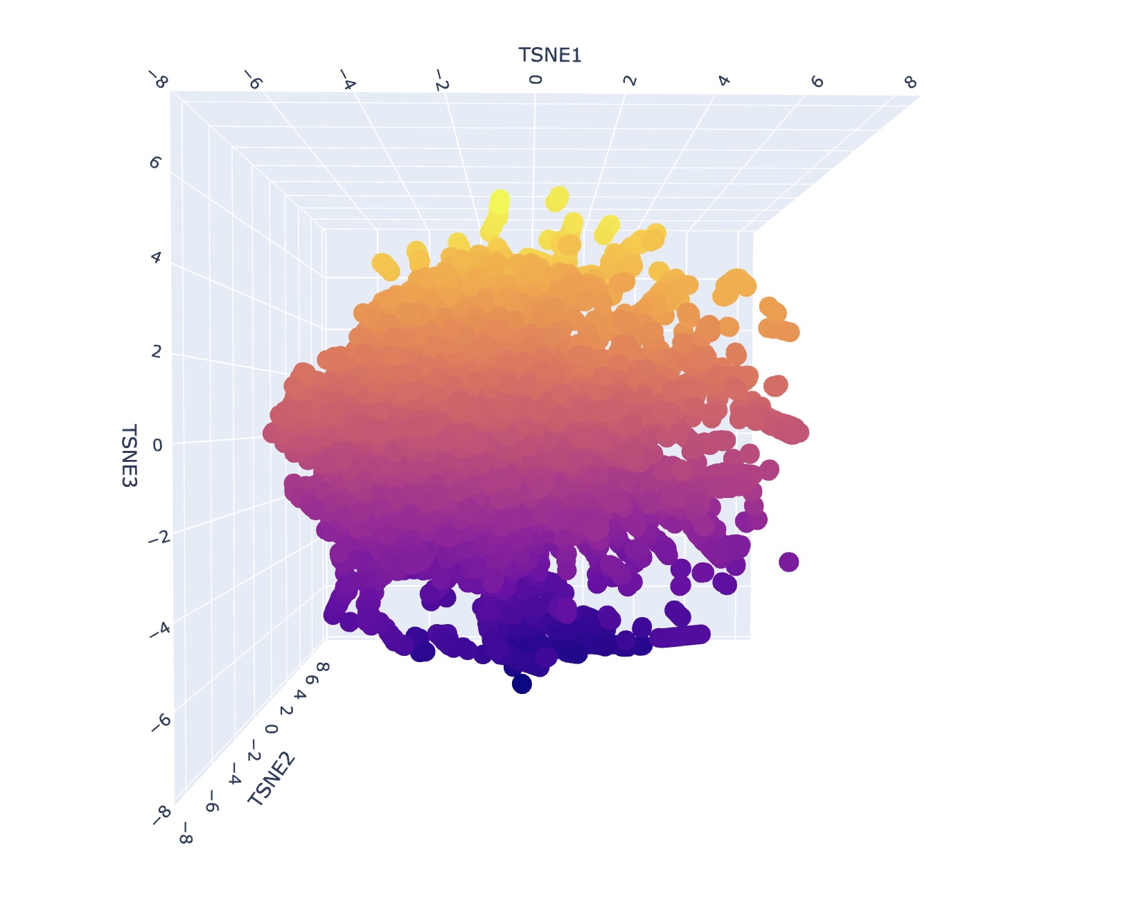
Latent Space Analysis
Use the provided sequence dataset to embed proteins in reduced dimensionality.
Analyze the different formed neighborhoods: do they approximate similar proteins?
I generally could not find super consistent themes or narratives when looking at different neighborhood clusters. I think this is reflective of how protein structure might appear similar but depending on the environment can have significantly different functional attributes. However, upon a second search, I saw that some families contained only bacterial proteins/prokaryotes. Some families also contained only human proteins or proteins of mammals.
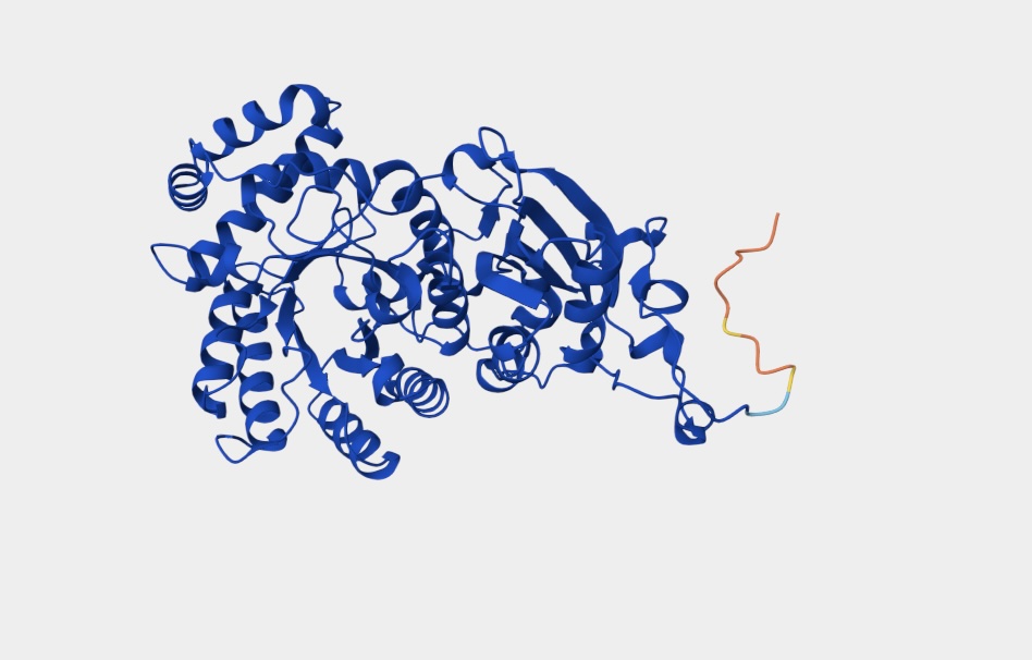
Folding a Protein
Fold your protein with ESMFold. Do the predicted coordinates match your original structure?
The predicted coordinates are similar to my original structure but not a perfect match.
Try changing the sequence, first try some mutations, then large segments. Is your protein structure resilient to mutations?
The protein structure is not resilient to mutations featuring distinct changes.
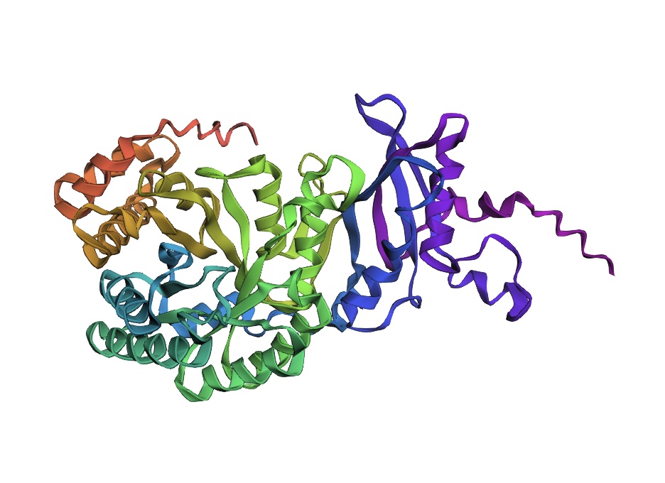
Inverse-Folding a Protein
Let’s now use the backbone of your chosen PDB to propose sequence candidates via ProteinMPNN.
Analyze the predicted sequence probabilities and compare the predicted sequence vs the original one.
Input this sequence into ESMFold and compare the predicted structure to your original.
The predicted structure is somewhat similar to the original structure indicating the viability of ESMFold readout for protein identification, modification, and discovery.
Week 5 Lab: Protein Design Part II
Lab Option 1: L-Protein Mutational Analysis
Experimental Validation & DMS
This lab provides a Deep Mutational Scanning (DMS) style validation of the L-Protein. By cross-referencing experimental lysis results—where a score of 1 indicates functional lysis and 0 indicates non-functional—with the Log-Likelihood Ratio (LLR) Heatmap generated via ESM2, we can assess the predictive power of protein language models.
Key Findings
Correlation: The agreement between the experimental data and the LLR Heatmap is remarkably high, approximately 90-95%.
Predictive Accuracy: The heatmap serves as a highly reliable predictor of whether a specific mutation will allow the protein to retain its ability to lyse bacterial cells.
Challenges: Designing mutants with high computational confidence remains difficult, highlighting the current limitations of some structure-based models.
Targeted Mutation Strategy
To identify promising variants, I cross-referenced the ESM2 scores with experimental lab data, specifically looking for residues that are not strictly conserved (via pBLAST) and show positive mutational effects.
Selection Criteria:
Soluble Region (N-tail): Targeted to assess how surface-exposed changes affect function.
Transmembrane Region: Targeted to test the hypothesis that the L-protein assembles to perforate the bacterial membrane.
Combined Effects: Testing synergistic effects of multiple “positive-score” mutations.
Proposed Mutants
Mutant
Substitution
Location
Index
Sequence Snippet
1
P –> Q
Soluble (N-tail)
6
METRFQQQSQQTPASTNRRRPFKHEDYPCRRNQRSST...
2
C –> S
Soluble (N-tail)
29
METRFPQQSQQTPASTNRRRPFKHEDYPSRRNQRSST...
3
S –> L
Transmembrane
49
...LYVLIFLAIFLLKFTNQLLLSLLEAVIRTVTTL...
4
K –> L
Transmembrane
50
...LYVLIFLAIFLSLFTNQLLLSLLEAVIRTVTTL...
5
C, K –> S, L
Combined
29 & 50
...PSRRNQRSSTLYVLIFLAIFLSLFTNQLLLSL...
Structural Hypothesis: Multimeric Assembly
A running hypothesis for L-protein function is that it assembles into a multimeric complex to create perforations in the bacterial membrane. To investigate this, I utilized AF2_Multimer to generate a predicted multimeric assembly.
By modeling these specific mutations (particularly those in the transmembrane region like Mutant 3 and 4) in a multimeric context, we can observe if the substitutions stabilize the pore-forming structure or increase the efficiency of membrane lysis.
Gemini AI was consulted for data organization and Markdown formatting
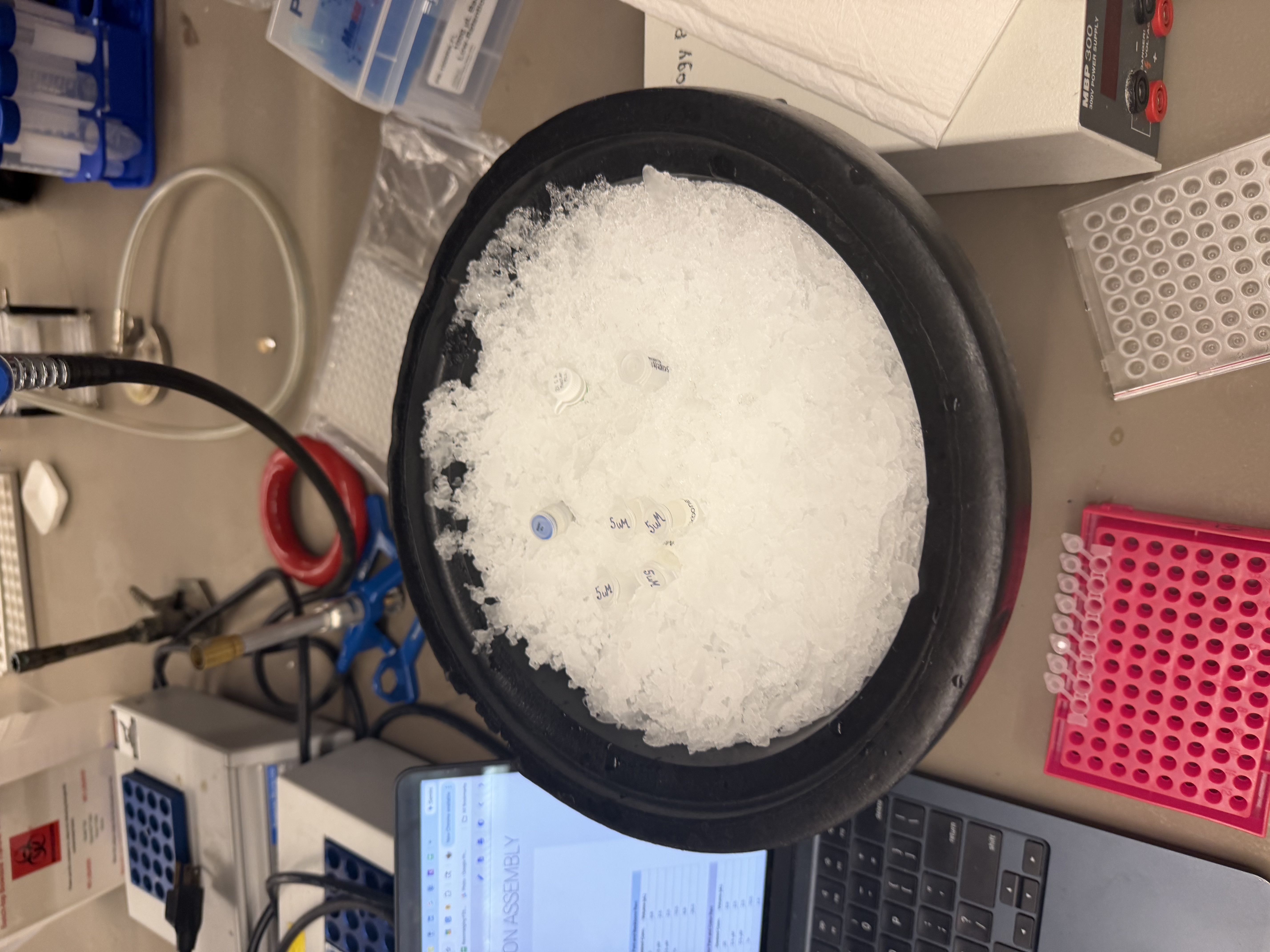
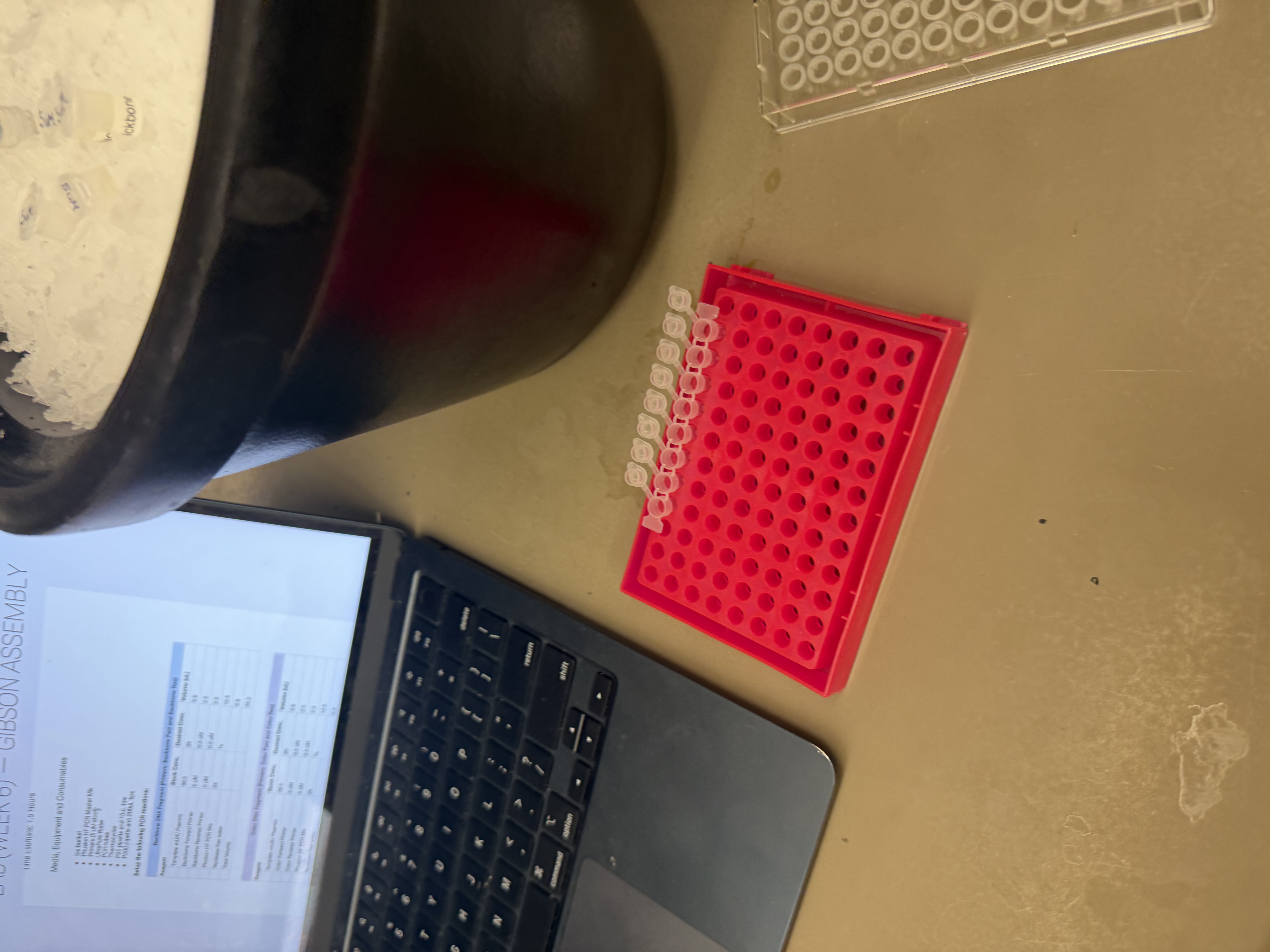
Week 6 Lab: Gibson Assembly
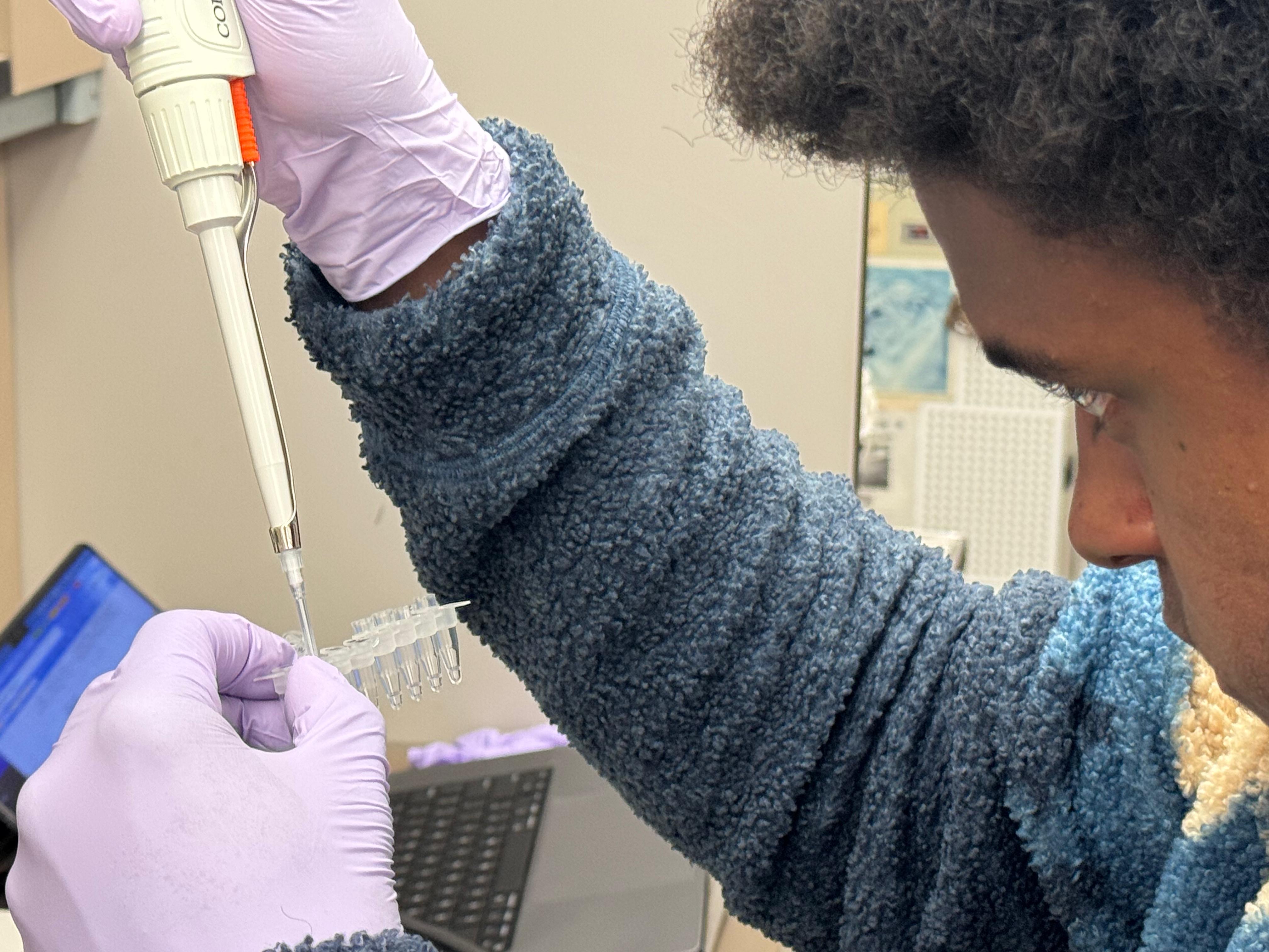
Day 1: Preparation of DNA Fragments
Background
In this two-day lab, we modified the color-generating chromophore of the purple Acropora millepora chromoprotein (amilCP) to create a variety of orange, pink, and blue mutants.
We performed two sets of Polymerase Chain Reactions (PCR) to prepare for a Gibson Assembly. The insert PCR region spans the 24 base pairs before the chromophore to just beyond the gene transcription terminator. The forward primer includes an intentional mismatch for site-directed mutagenesis of the mUAV DNA plasmid. These mutants were then expressed in chemically competent E. coli cells.
PCR Reaction Setup
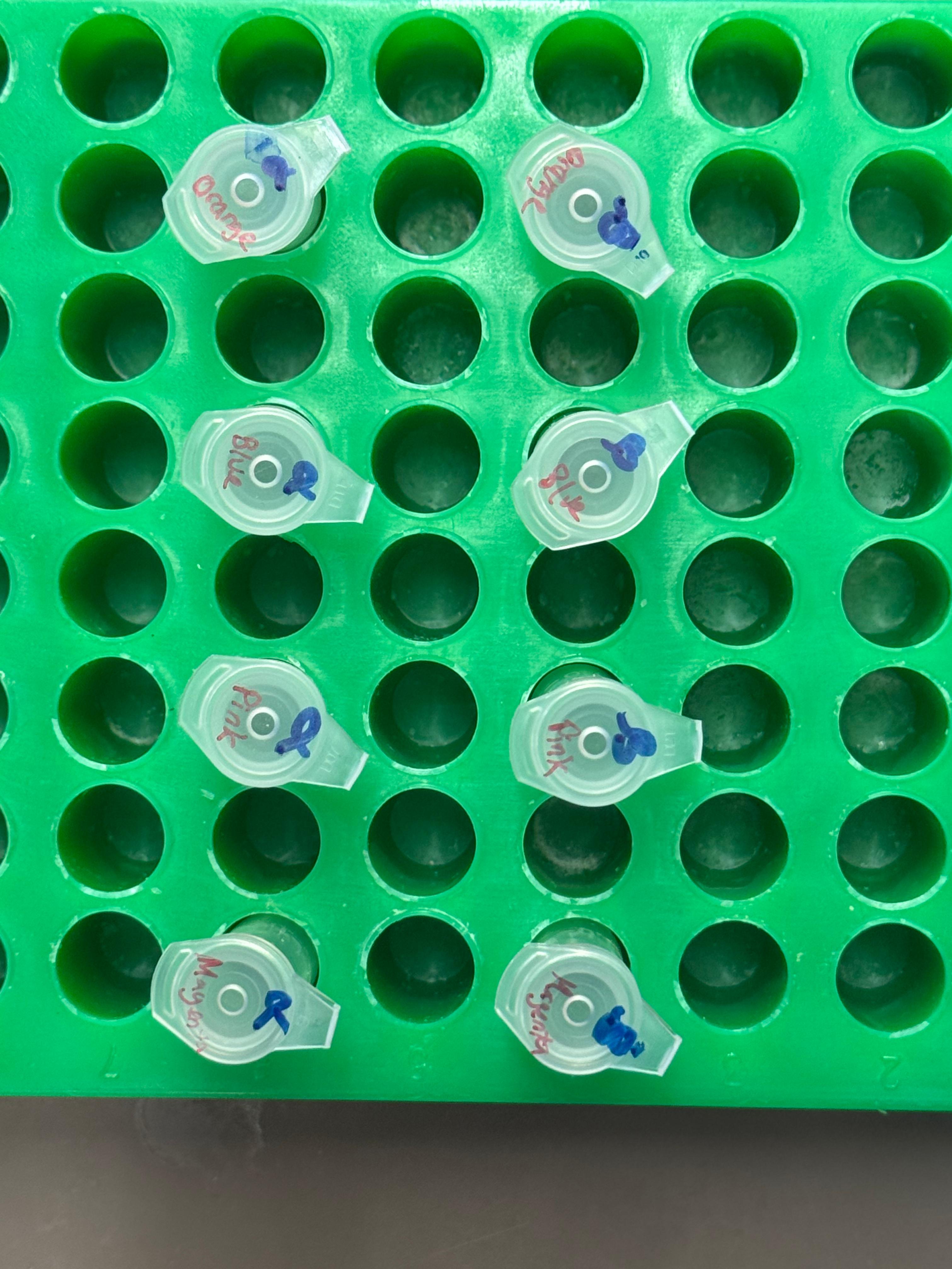
We prepared a backbone reaction alongside four color-specific reactions: Blue, Light Pink, Magenta, and Orange.
1. Backbone DNA Fragment
Primers: Backbone Fwd and Backbone Rev
Reagent
Stock Conc.
Desired Conc.
Volume (µL)
Template mUAV Plasmid
38.5 ng/µL
20 ng
0.8
Backbone Forward Primer
5 µM
0.5 µM
2.5
Backbone Reverse Primer
5 µM
0.5 µM
2.5
Phusion HF PCR Mix
2X
1X
12.5
Nuclease-free water
—
—
6.8
Total Volume
—
—
25.0
2. Color DNA Fragments
Primers: Color Fwd and Color Rev
Reagent
Stock Conc.
Desired Conc.
Volume (µL)
Template mUAV Plasmid
38.5 ng/µL
20 ng
0.8
Color Forward Primer
5 µM
0.5 µM
2.5
Color Reverse Primer
5 µM
0.5 µM
2.5
Phusion HF PCR Mix
2X
1X
12.5
Nuclease-free water
—
—
6.8
Total Volume
—
—
25.0
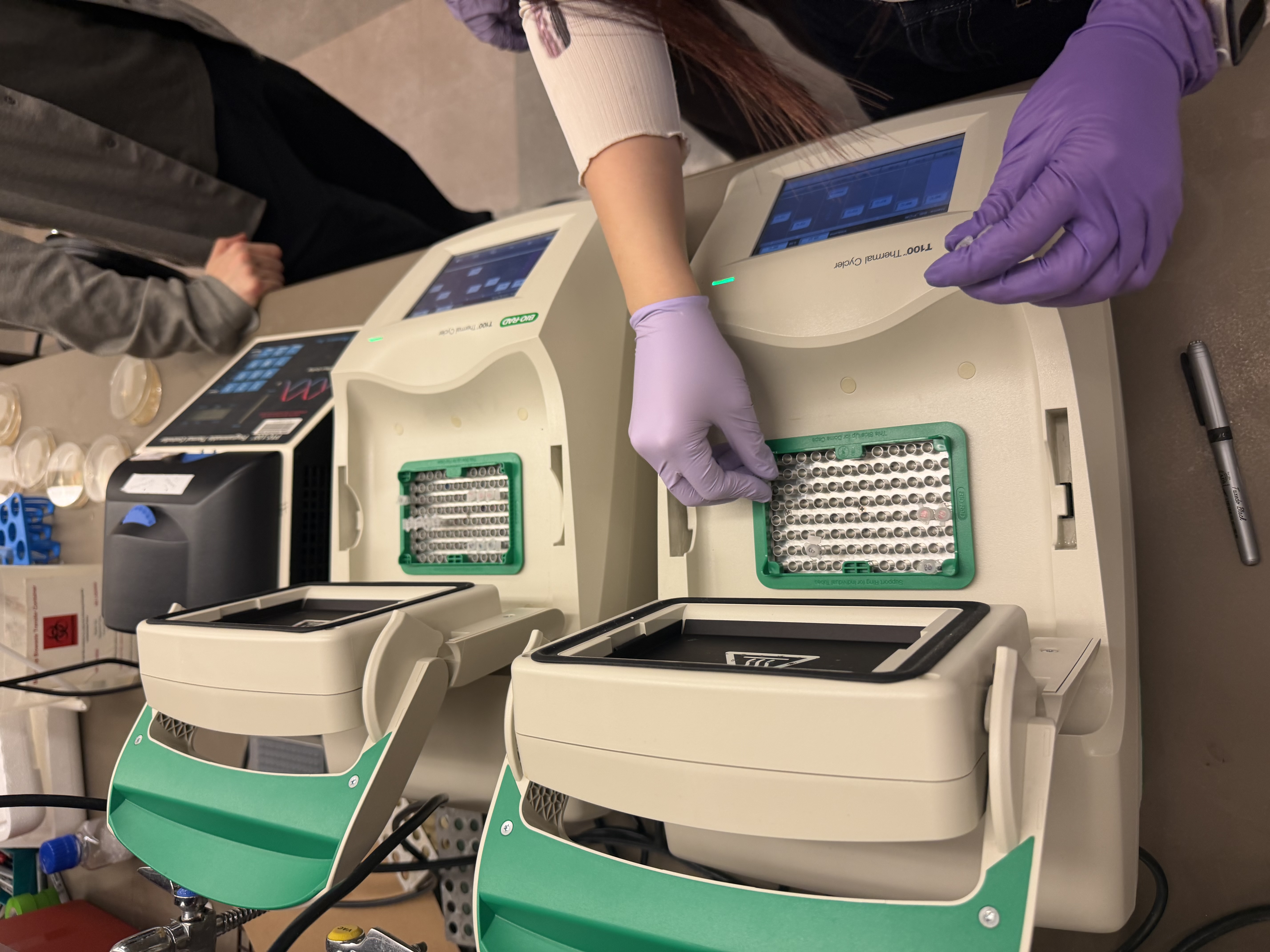
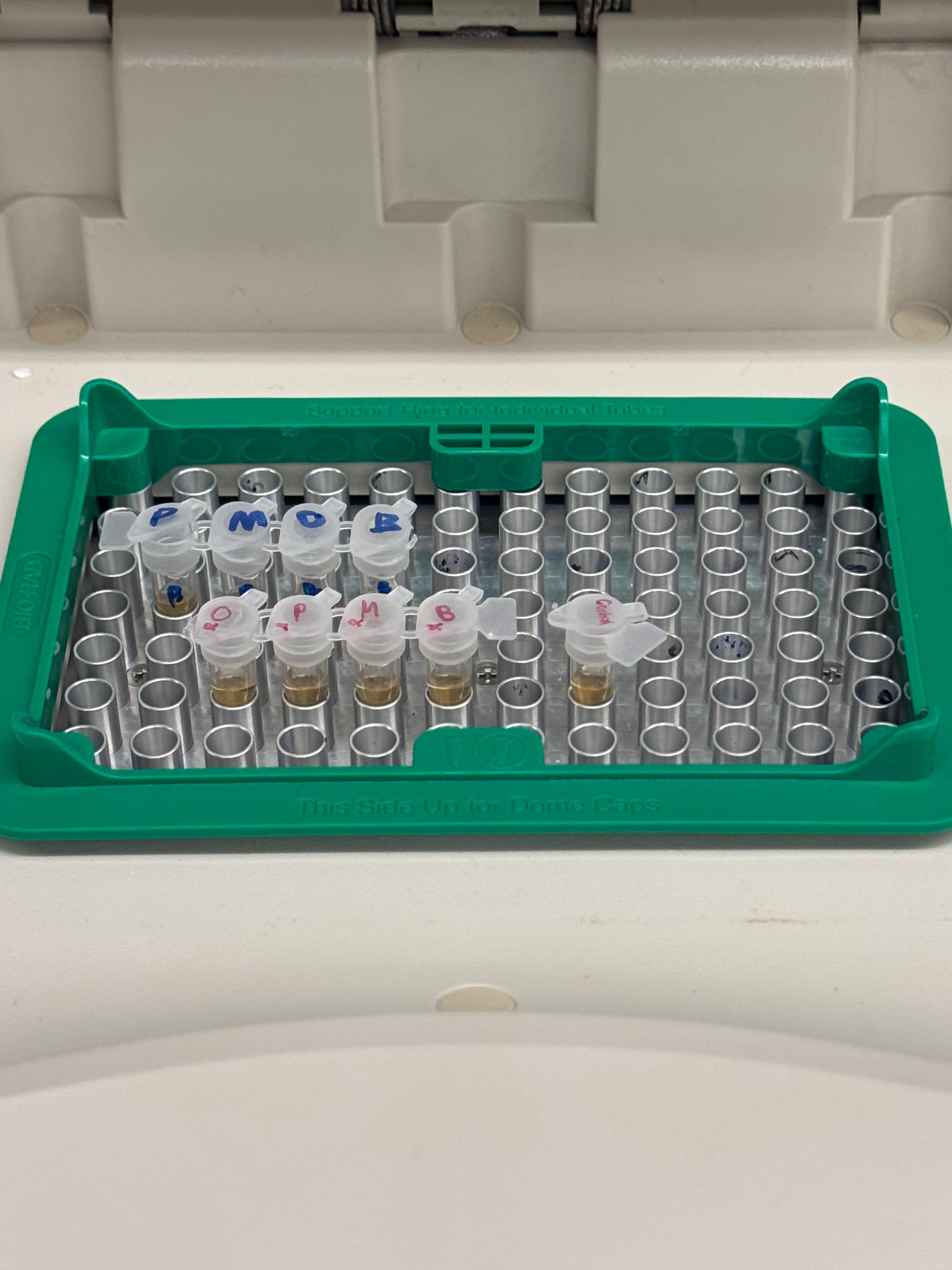
After mixing, the tubes were placed in the thermocyclers. The backbone was run on one specialized program while the color mutations were run on another.
Note: DpnI digest was skipped as our reactions did not contain methylated DNA.
Purification & Analysis
We purified the PCR products using the Zymo DNA Clean & Concentrator kit.
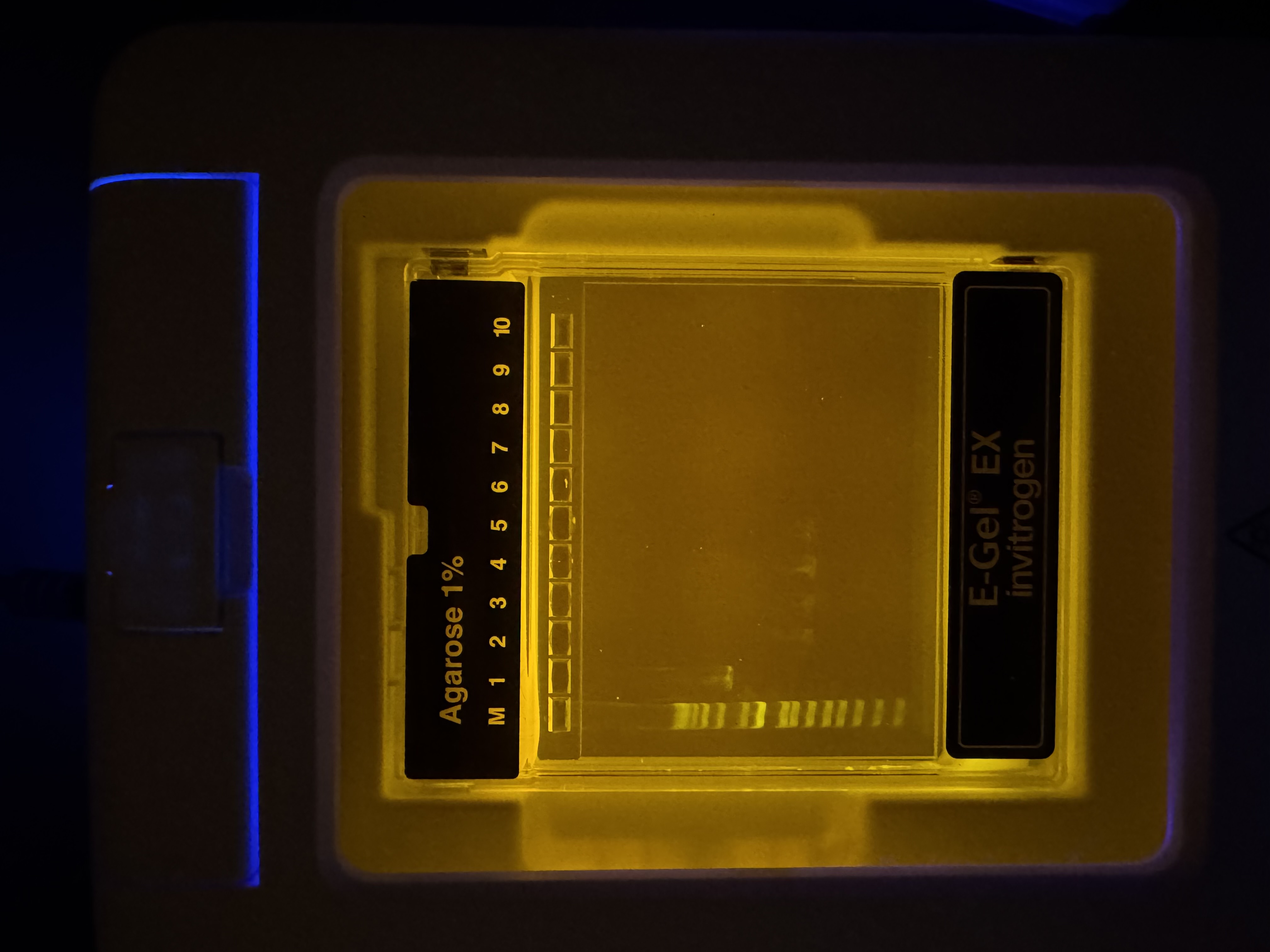
We utilized Zymo-Spin columns, performed two washes, and eluted the DNA for storage. The listed protocol was for 50µL of PCR product. We made 25µL total in our PCR reactions, so we used 20µL of PCR product (saved 5µL) in the purification process and scaled the other volumes to equal proportion. Gel electrophoresis was performed to verify the amplification.
Gel Results: We had a 1kb ladder furthest left, and Lane 1 contains the native plasmid. Lanes 2–5 show the expected amplified fragments for the Gibson Assembly, all roughly around 650bp. Our gel results were very convincing, we didn’t see formation of primer dimers or miscellaneous bands indiciating reduced PCR efficacy and polymerase fideltiy. Each sample contained a strong band at the expected bp length. Samples were then stored in fridge until the next lab day.
Day 2: Assembly & Transformation
Gibson Assembly
We diverged slightly from the standard protocol by utilizing unpurified PCR products for the assembly. This decision was made for a couple of reasons. We realized we had very small samples of each color in both the purified and unpurified results, effectively forcing us to chose between assaying the concentration via nano-drop or assembling the reaction with our theoretical maxium concentration. Additionally, other groups were reporting very low (almost negligible) concentrations when they tested purified PCR products. So, we decided to use our unpurified products and followed the rest of the protocol as stated (given our gel result, we deemed it reasonable to assume that the majority of DNA content was the desired amplicon.
Reagent
Stock Conc. (ng/µL)
Desired Conc (ng/µL)
Volume (µL)
Backbone Fragment
50
25
0.5
Color Fragment (Single)
50
50
1.0
Gibson Assembly Mix
2X
1X
5.0
Nuclease-free water
—
—
3.5
Total Volume
—
—
10.0
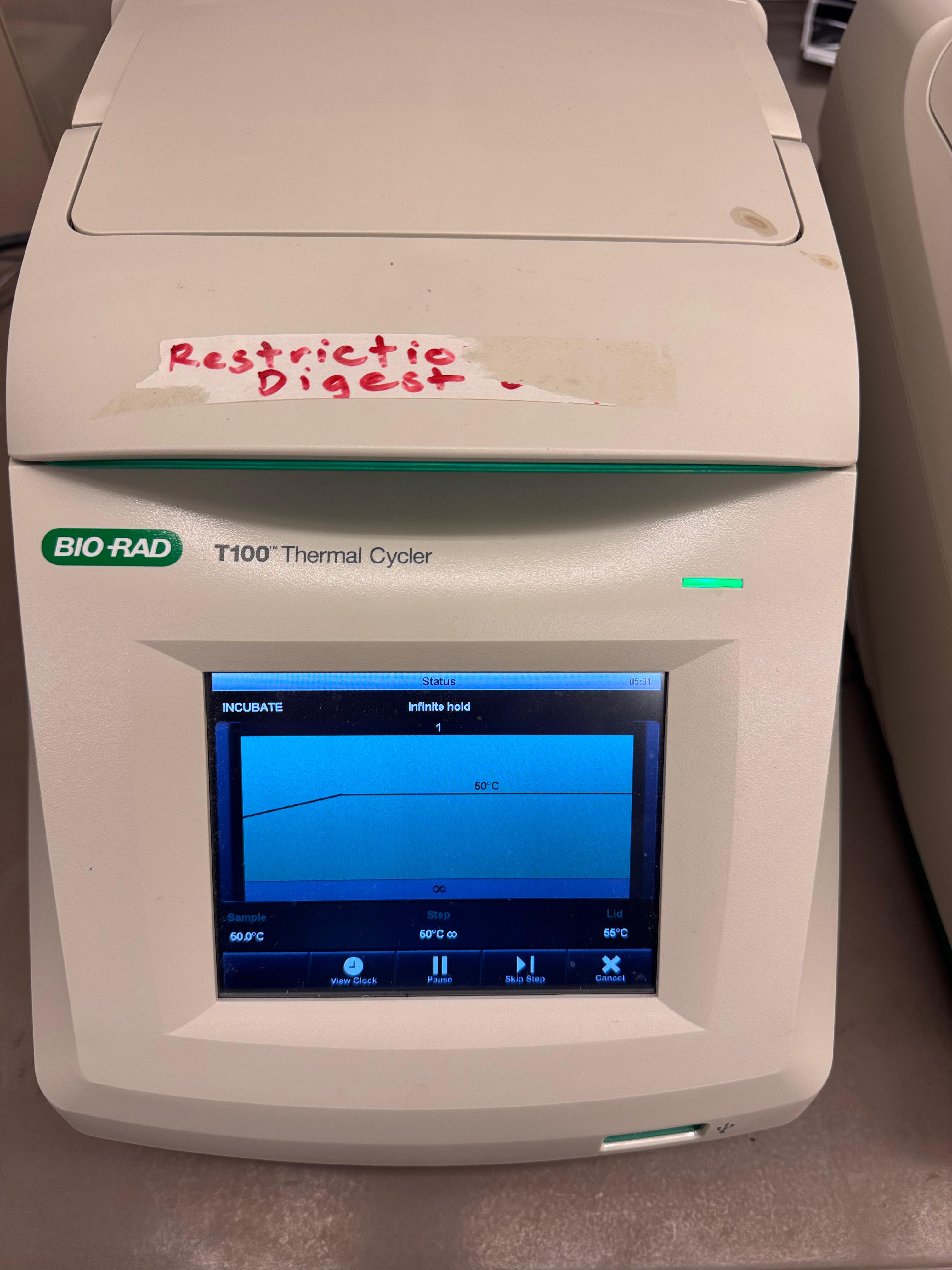
The reaction was incubated at 50°C in the thermocycler for 30 minutes.
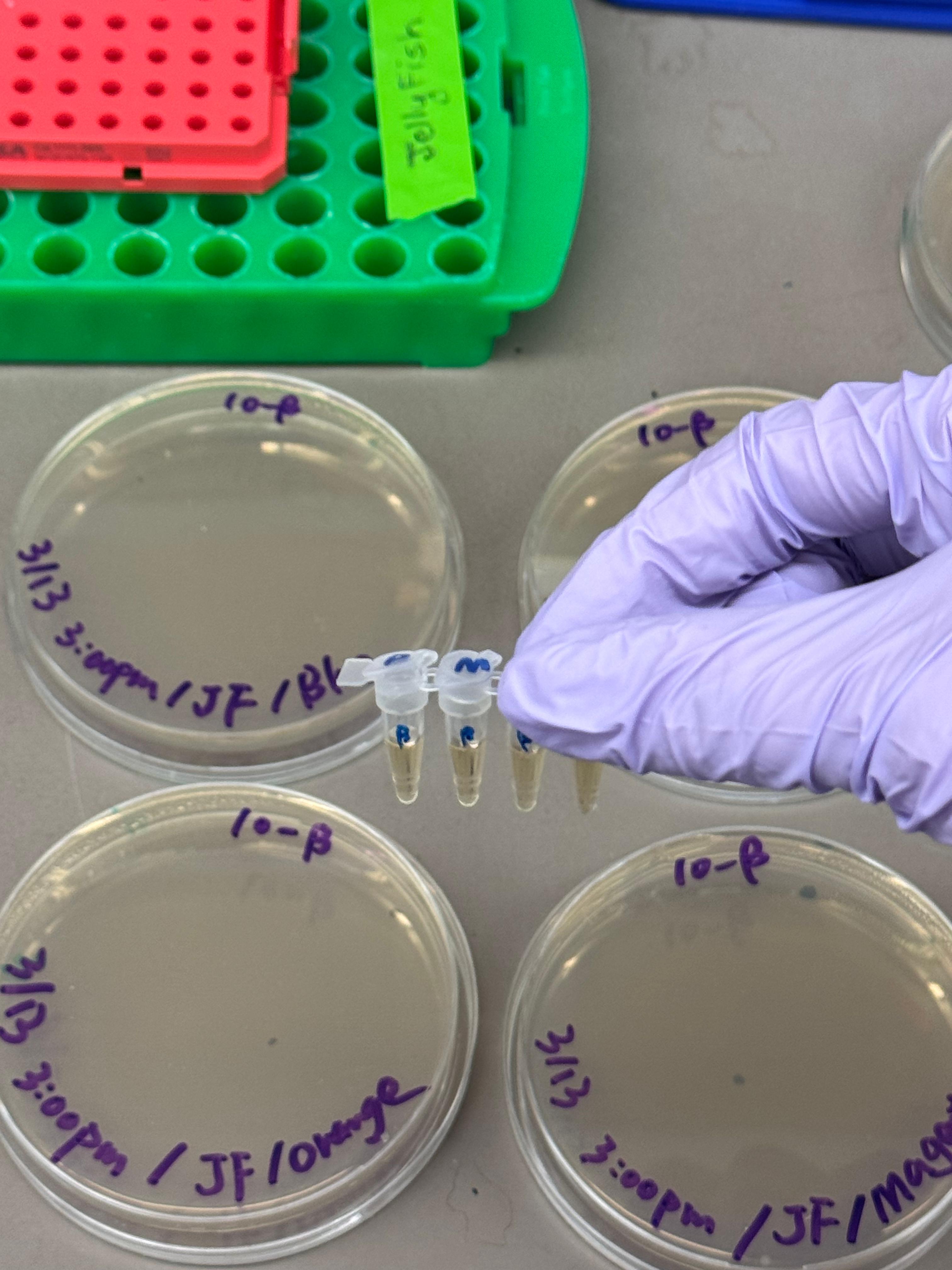
Transformation
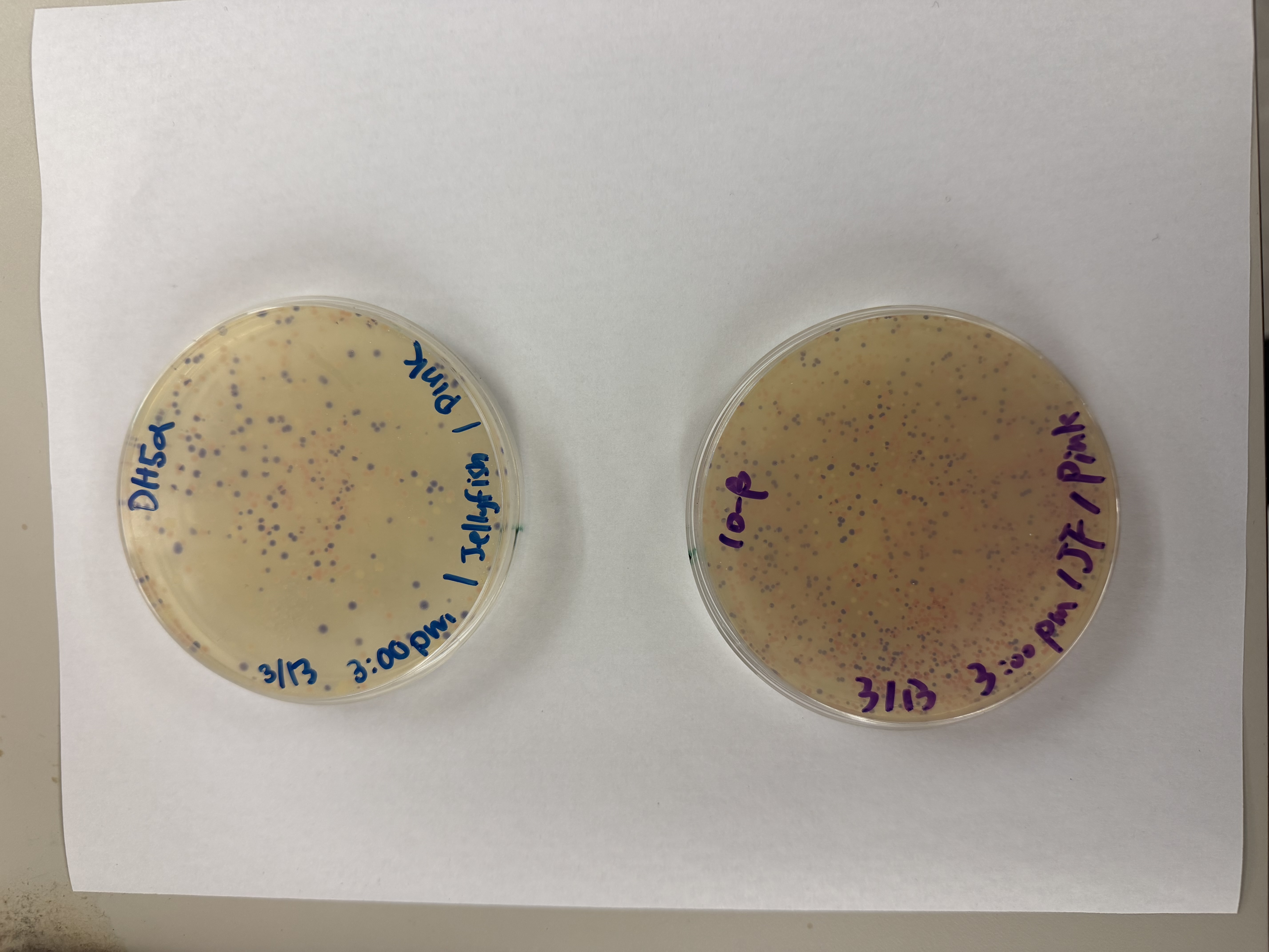
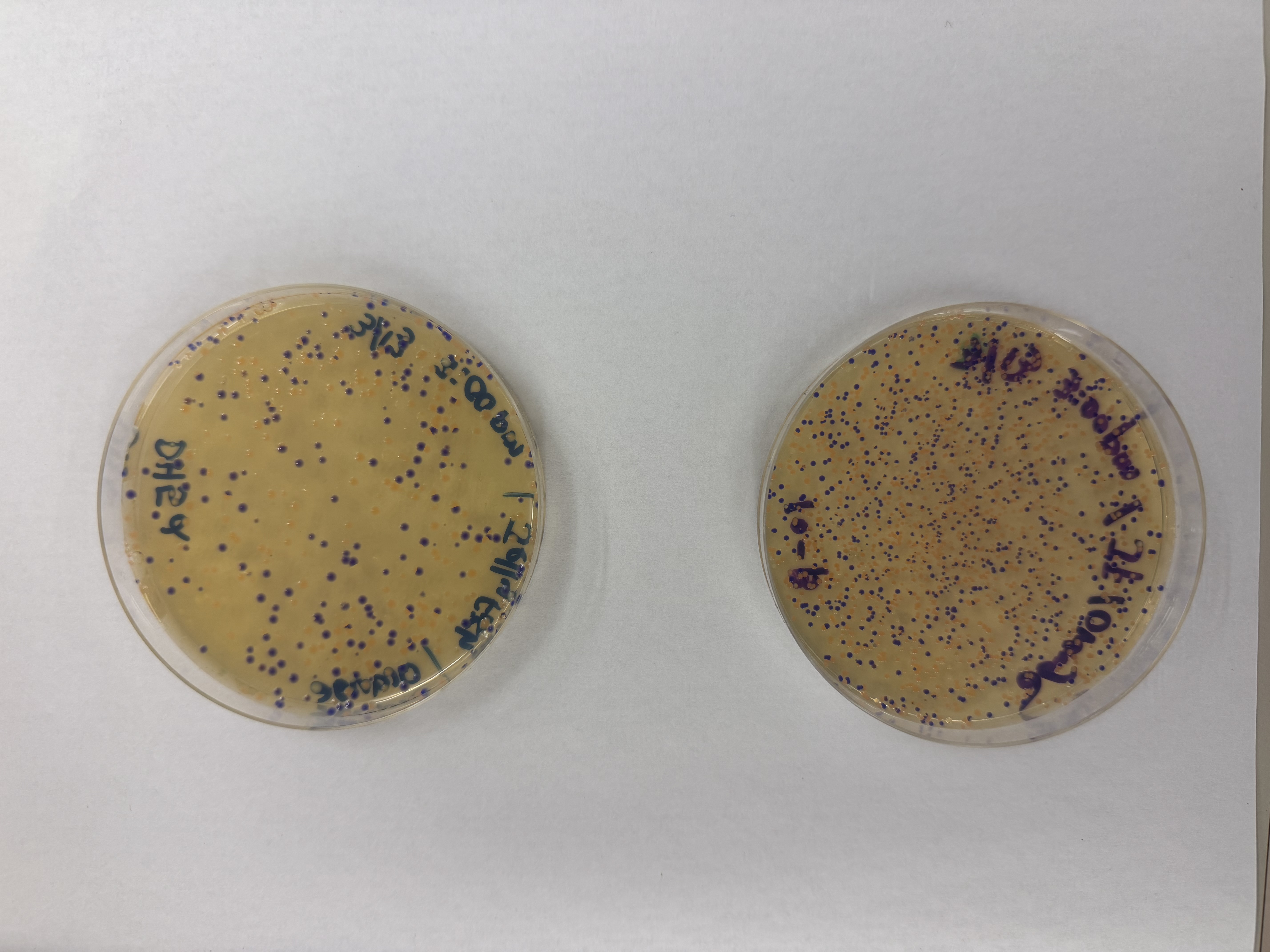
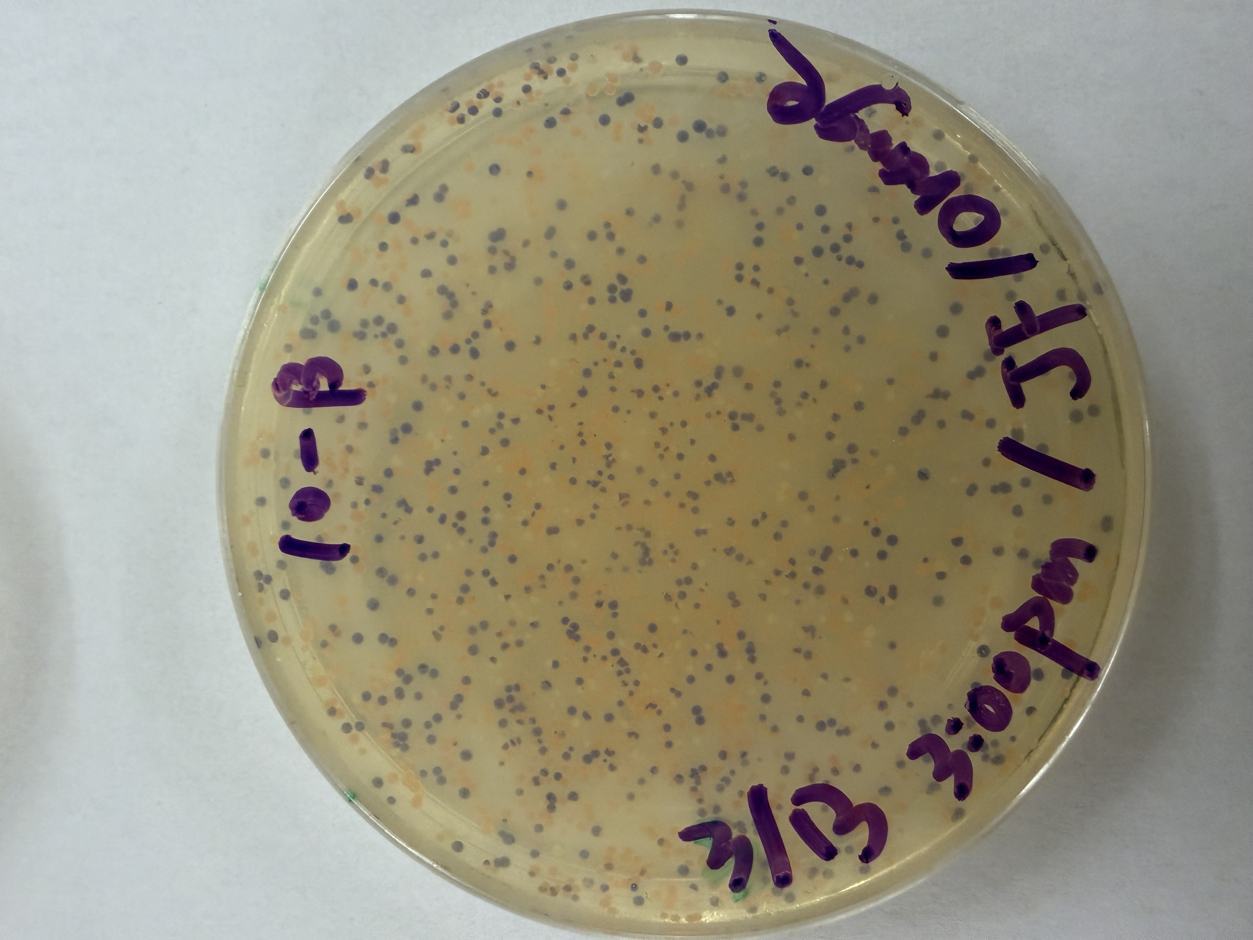
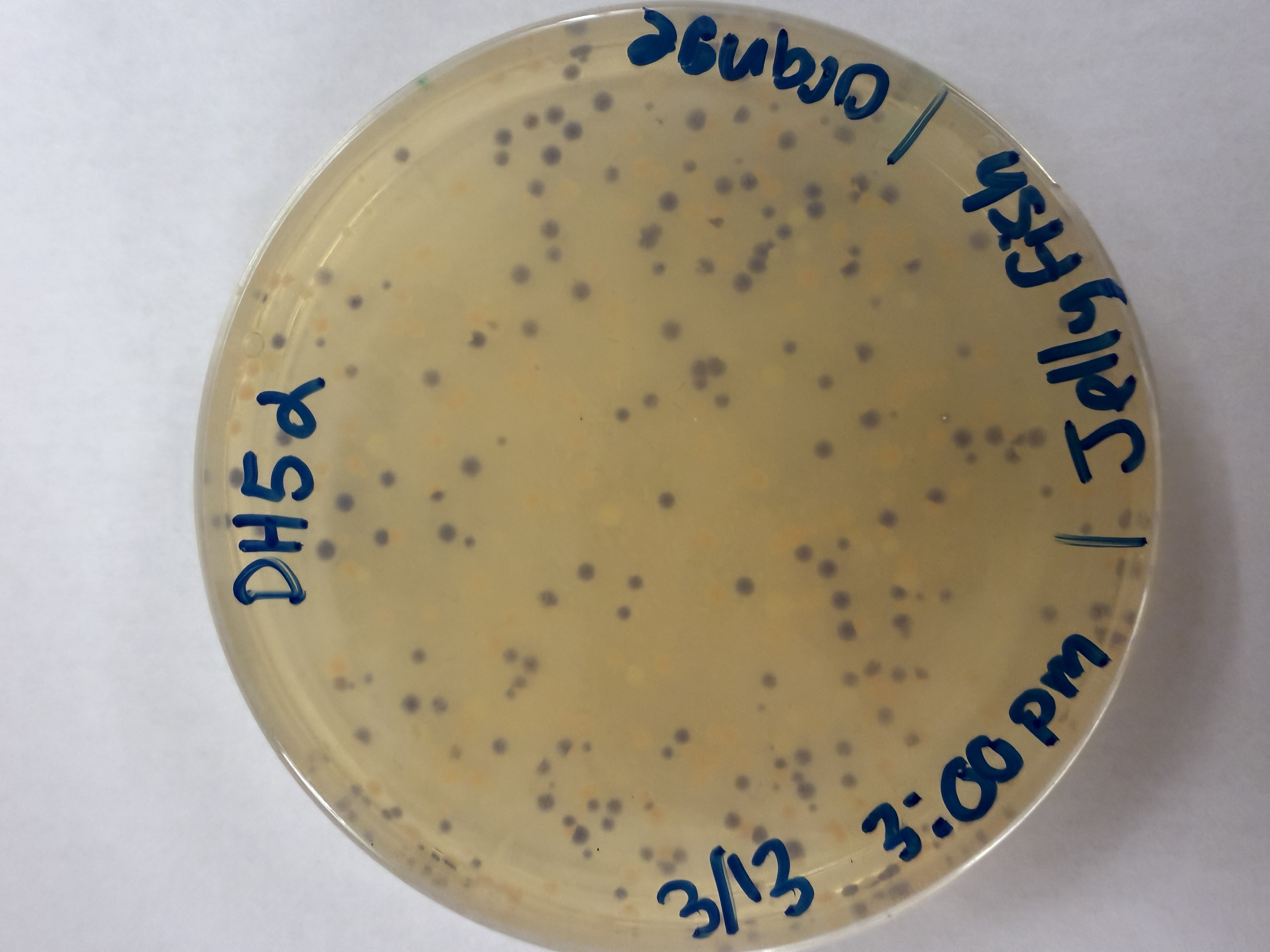
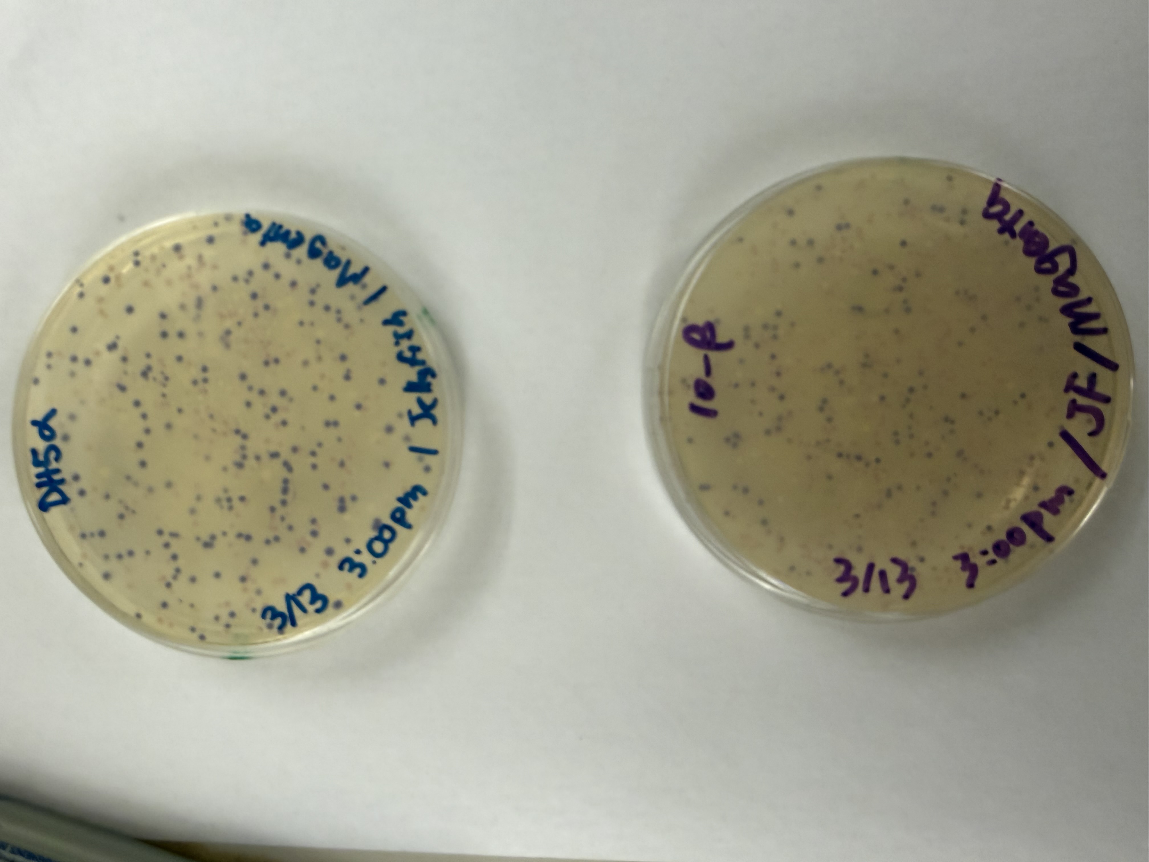
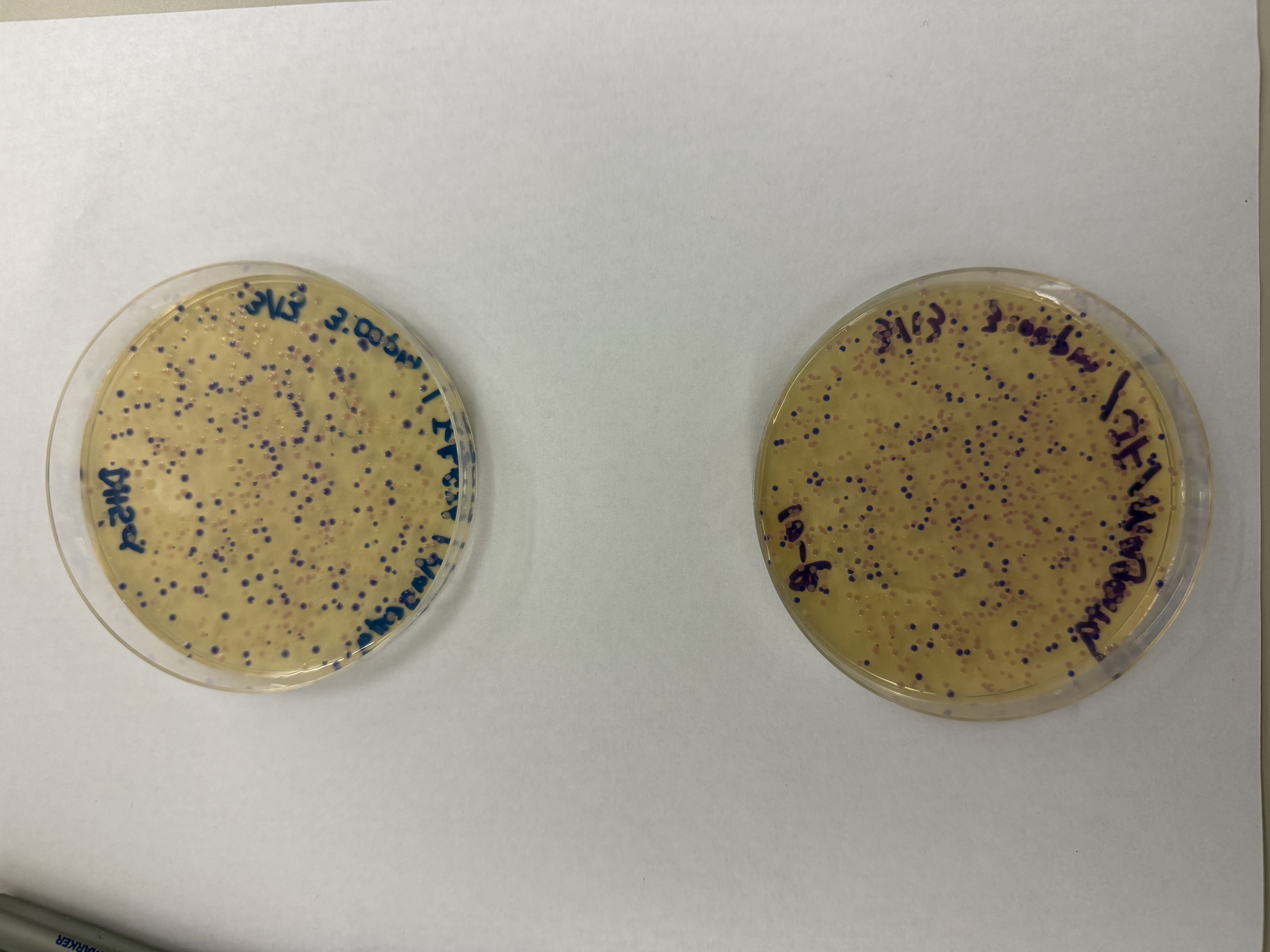
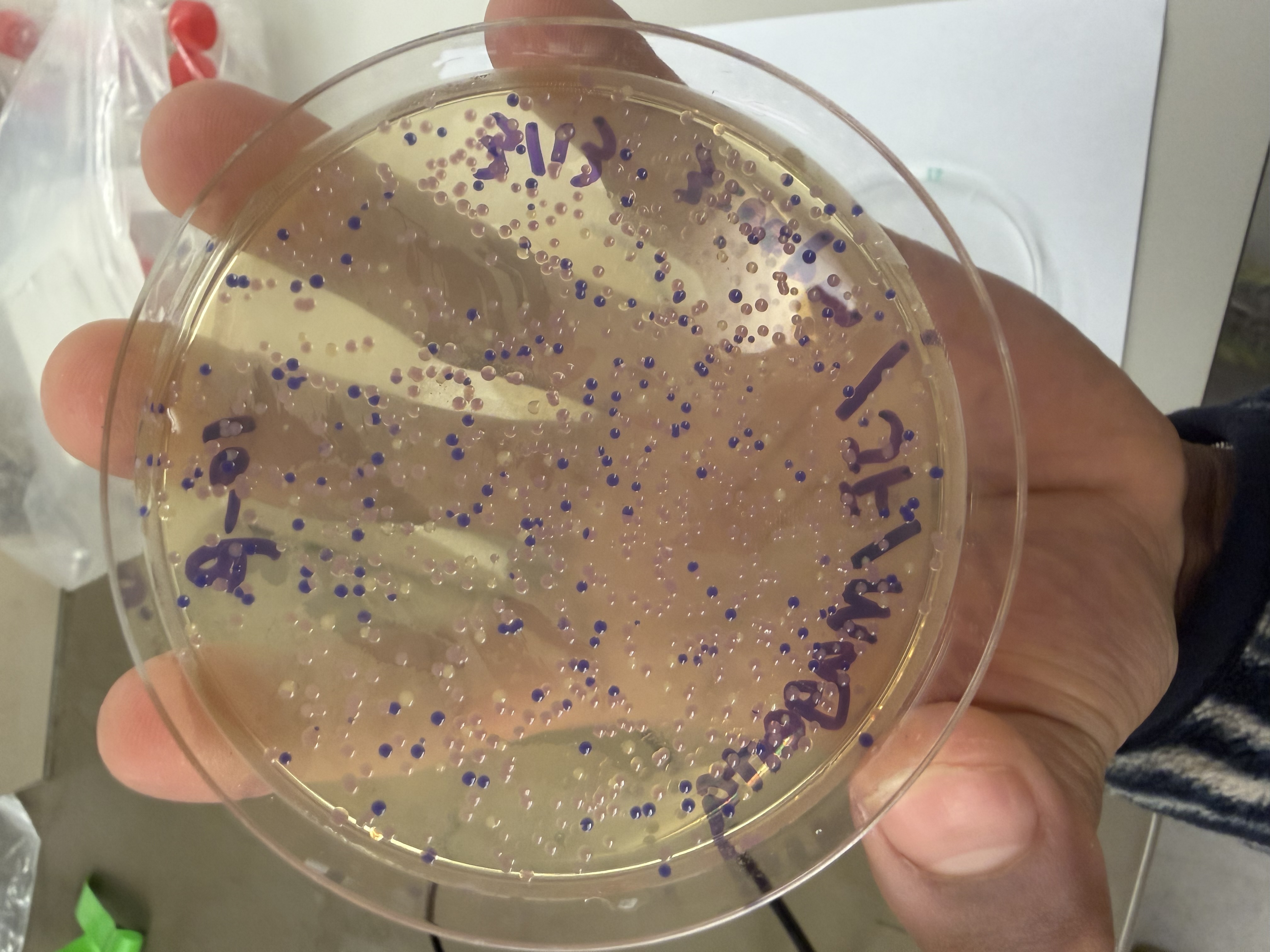
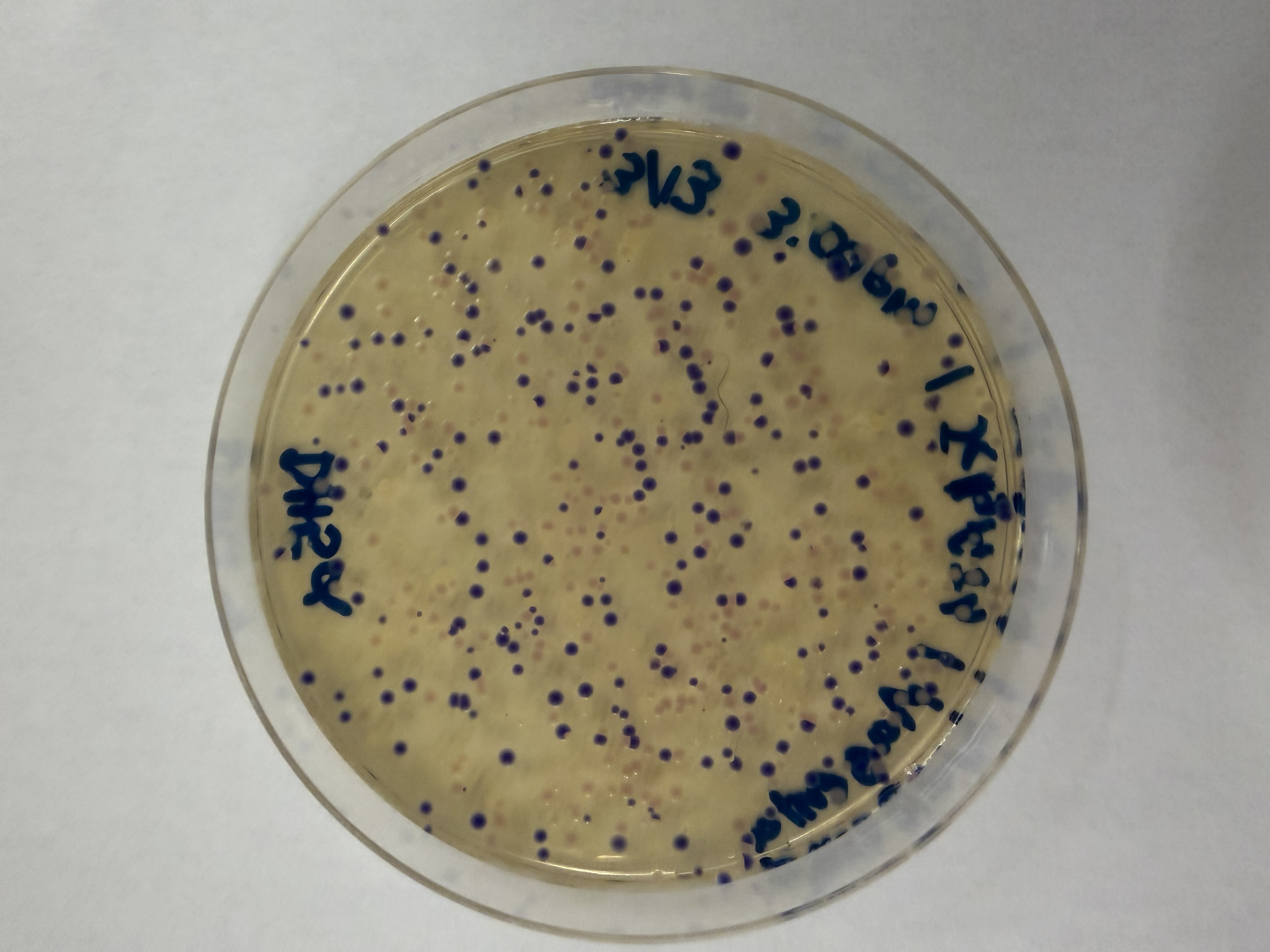
We compared two competent E. coli strains: DH5α and 10-beta.
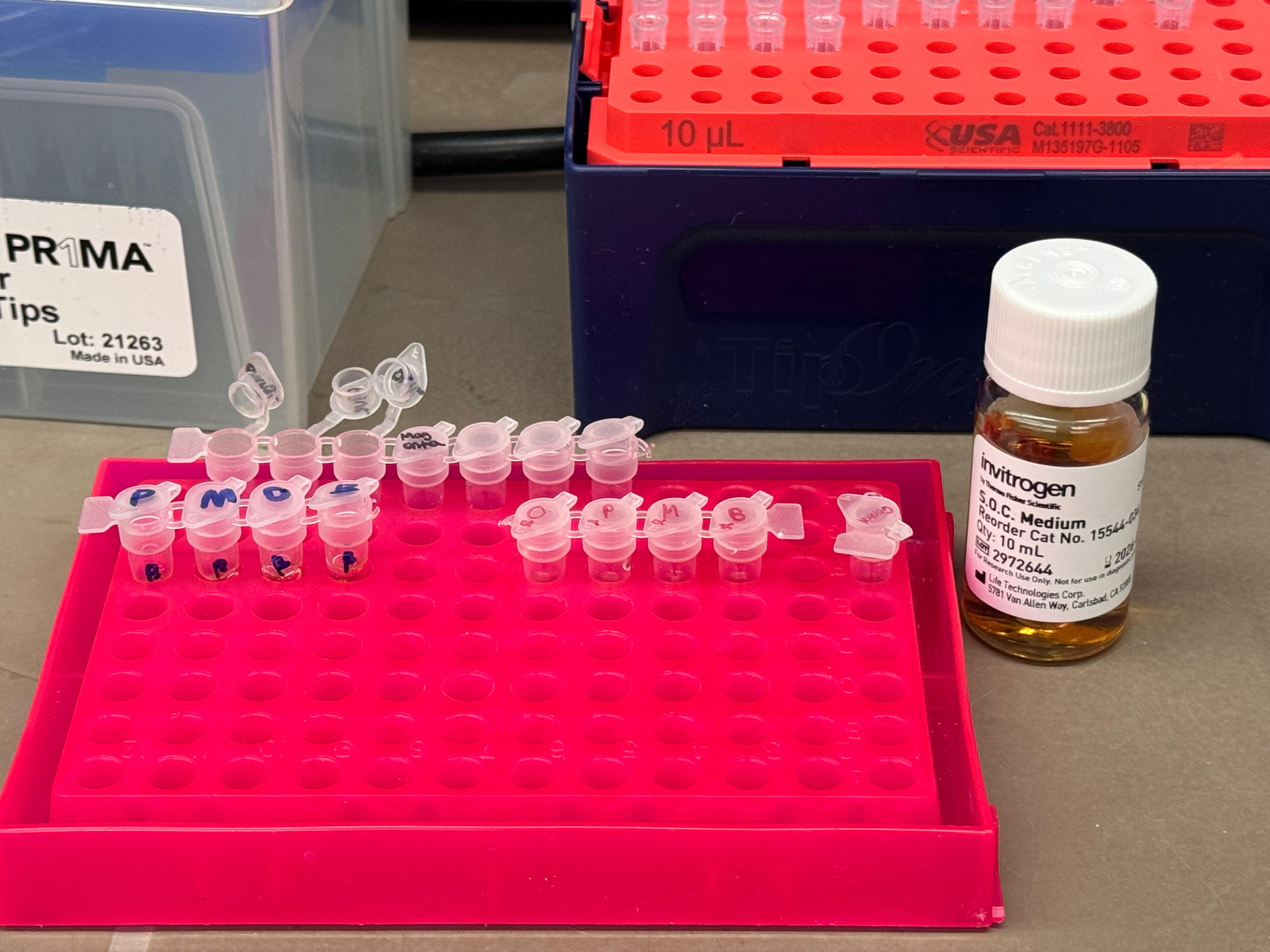
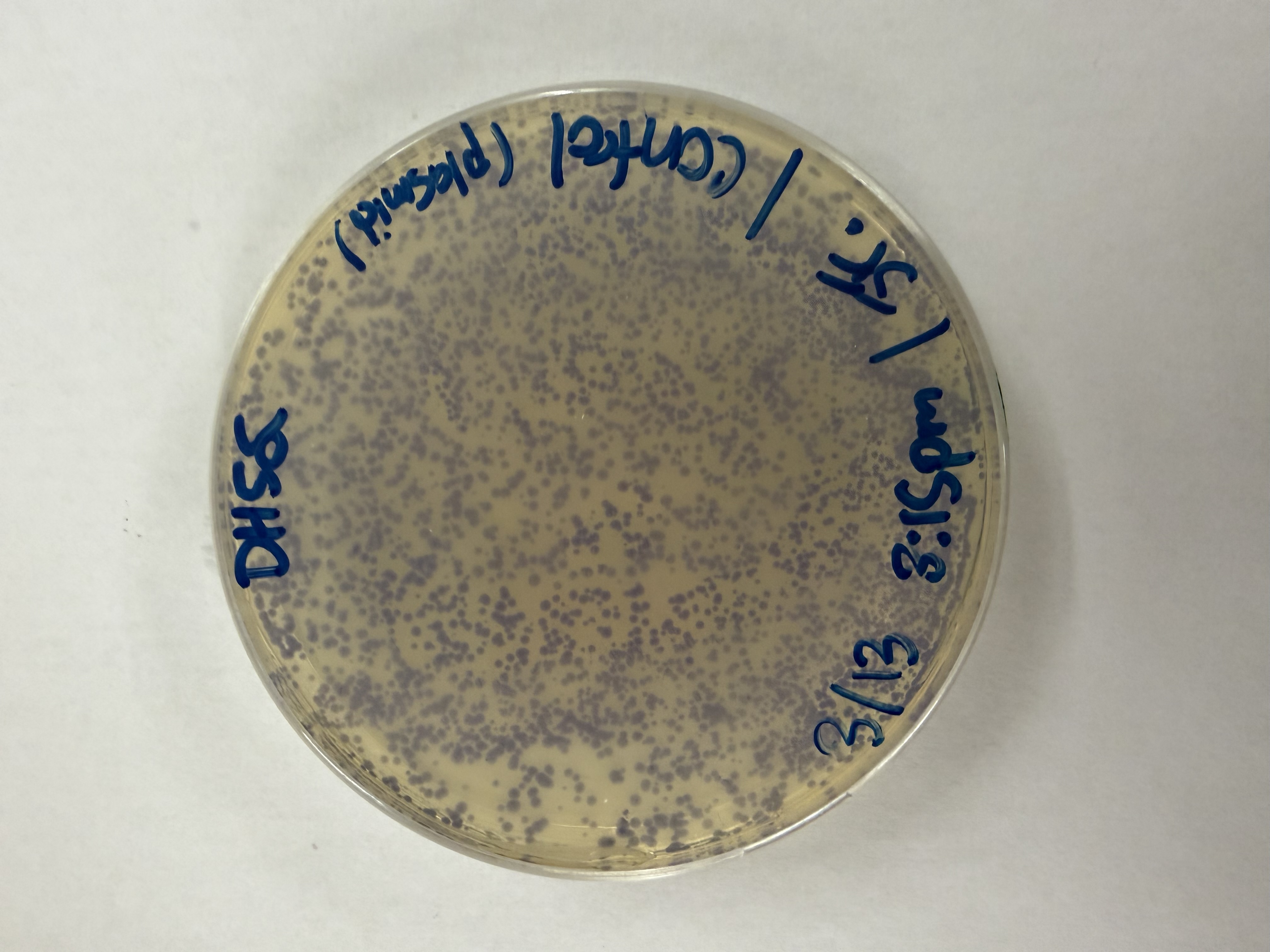
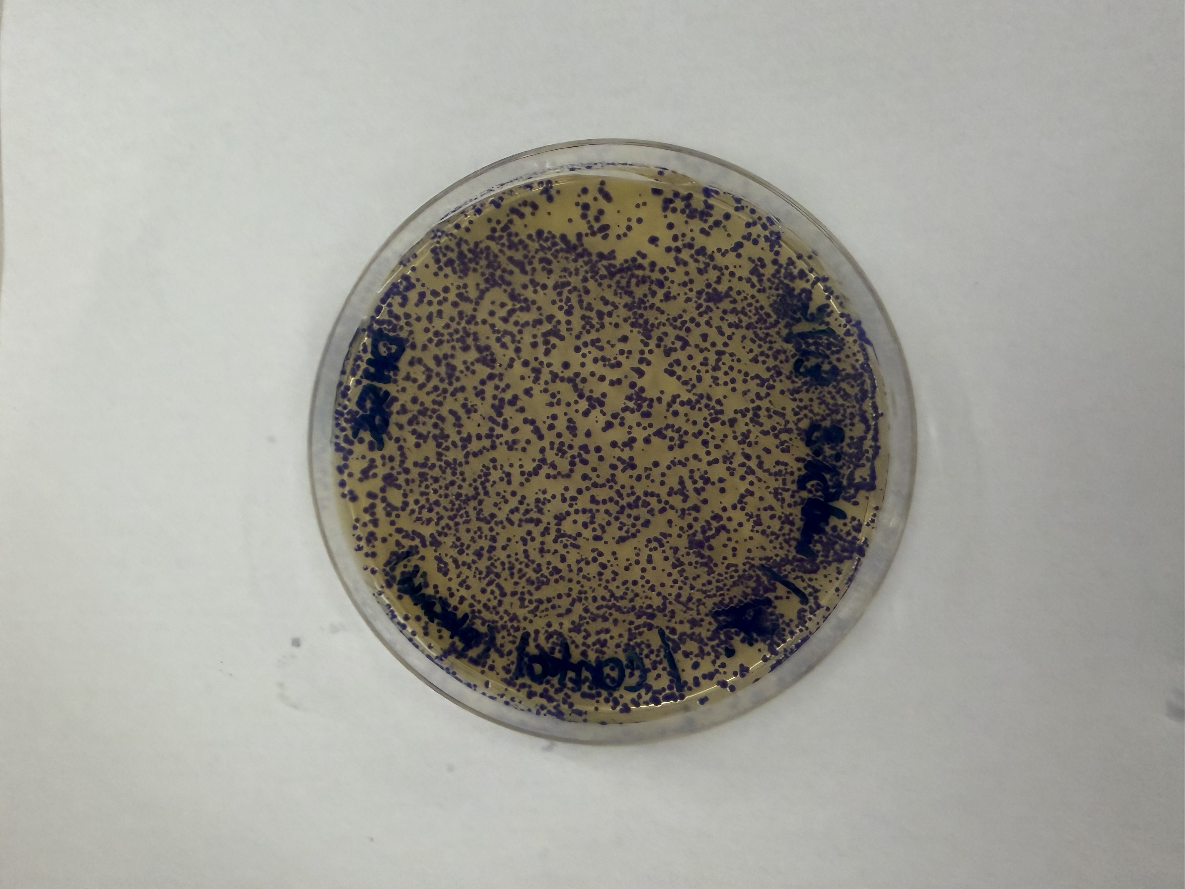
We thawed our competent cells, and mixed 20µL of cells with 4µL from each of our Gibson Assembly reactions and incubated for 30 minutes on ice. We also did an additional reaction with just the native plasmid (DH5α with mUAV) to serve as a positive control for successful transformation. To create the control, I only utilized 1µL of the plasmid to try and somewhat match the total concentration of the samples.
At this next step, we again diverged slightly from the protocol. We transfered the transformation reactions into PCR tubes containing 100µL of SOC medium and performed the heat shock step in that solution in the thermocycler. The heat shock importantly was only 45 seconds, and the cells were put on ice immediately after.
Incubation: Mixed competent cells with Gibson products and incubated on ice for 30 minutes.
Heat Shock: Performed in the thermocycler for 45 seconds in SOC medium, then immediately returned to ice.
Outgrowth: Incubated for 60 minutes (it was really ~45 minutes) using a makeshift shaker made from a pipette tip box.
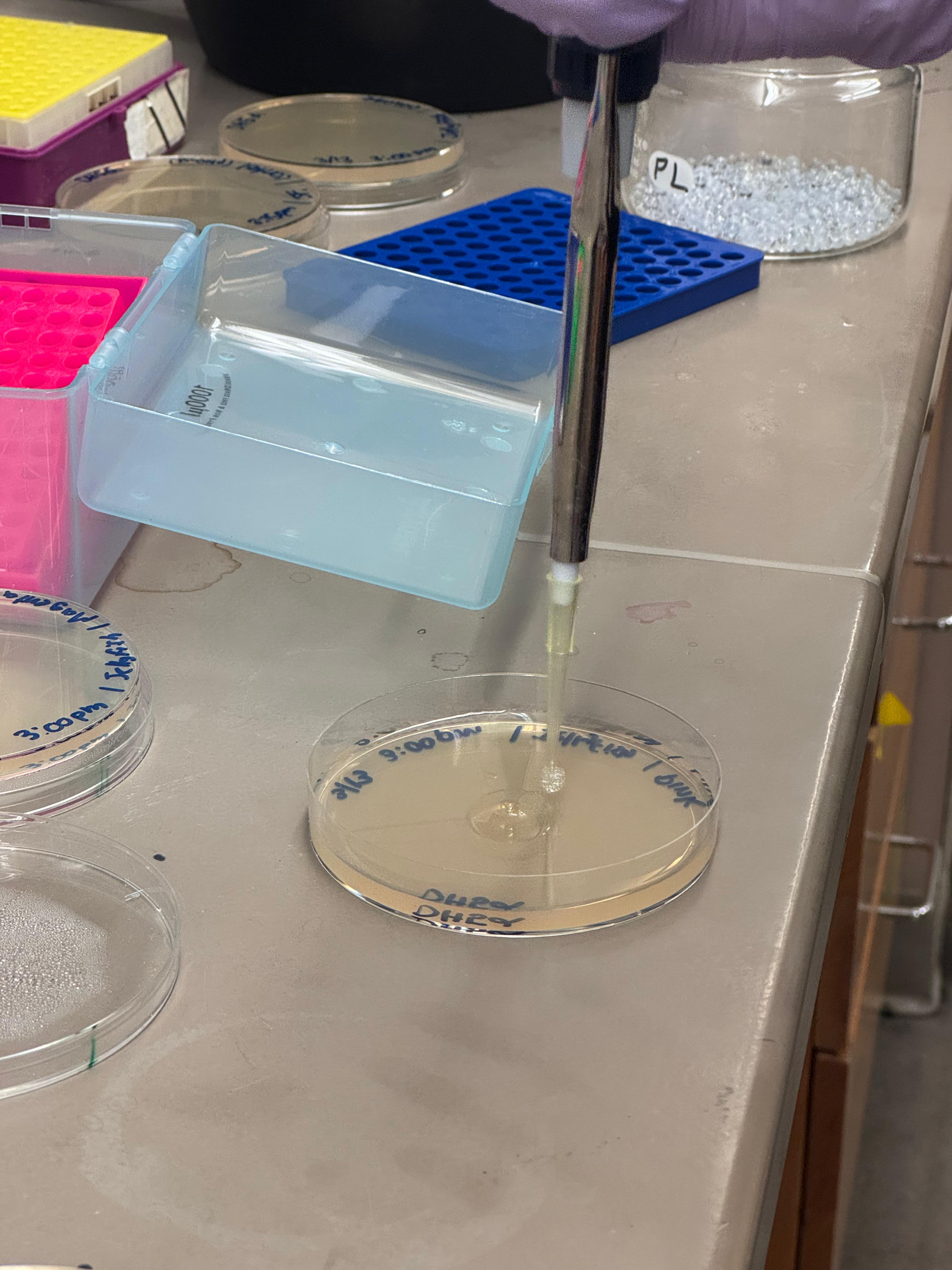
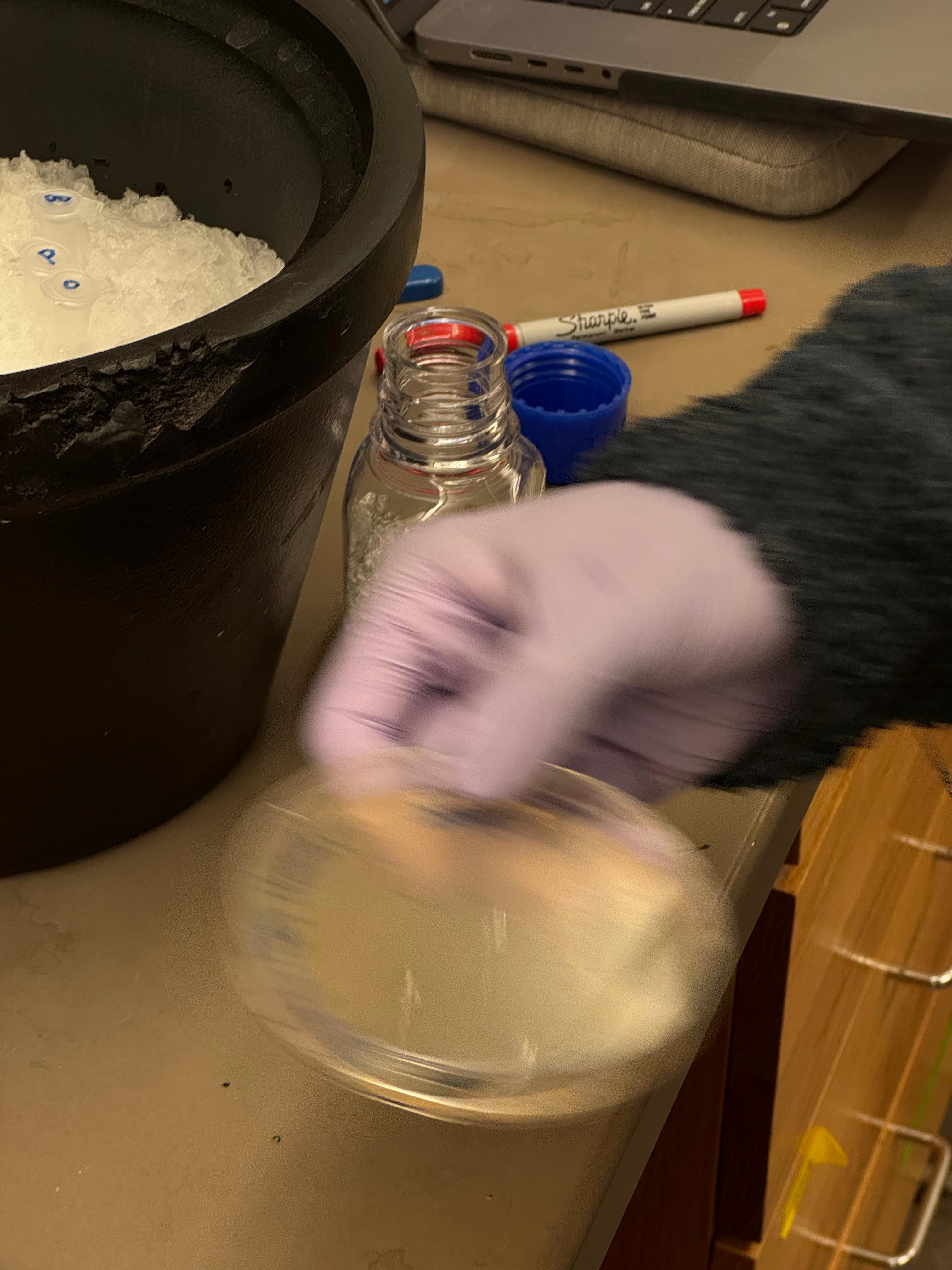
We plated the entire incubation (~124µL) of each transformation onto LB-Agar plates with Chloramphenicol using glass beads for even spreading.
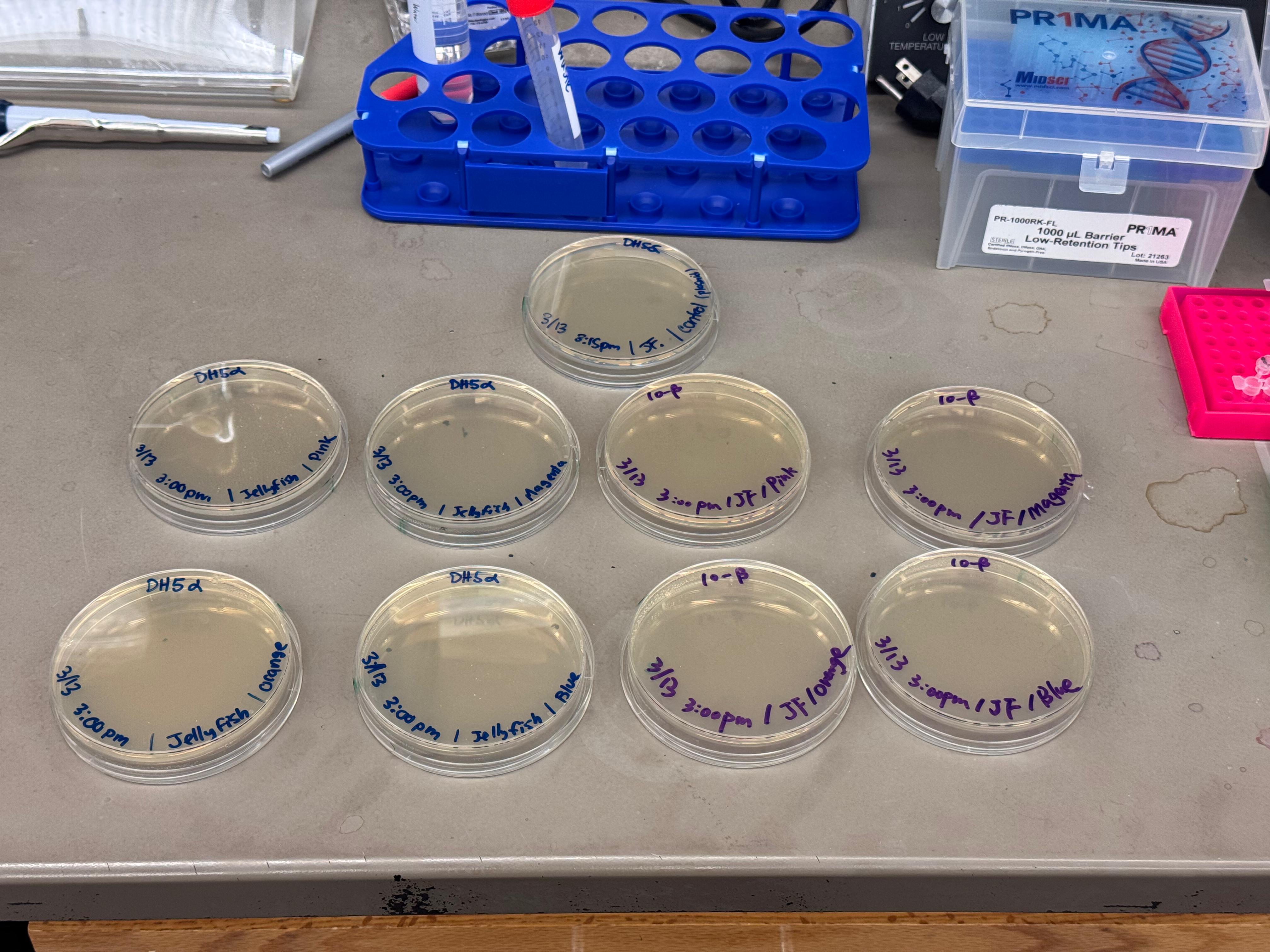
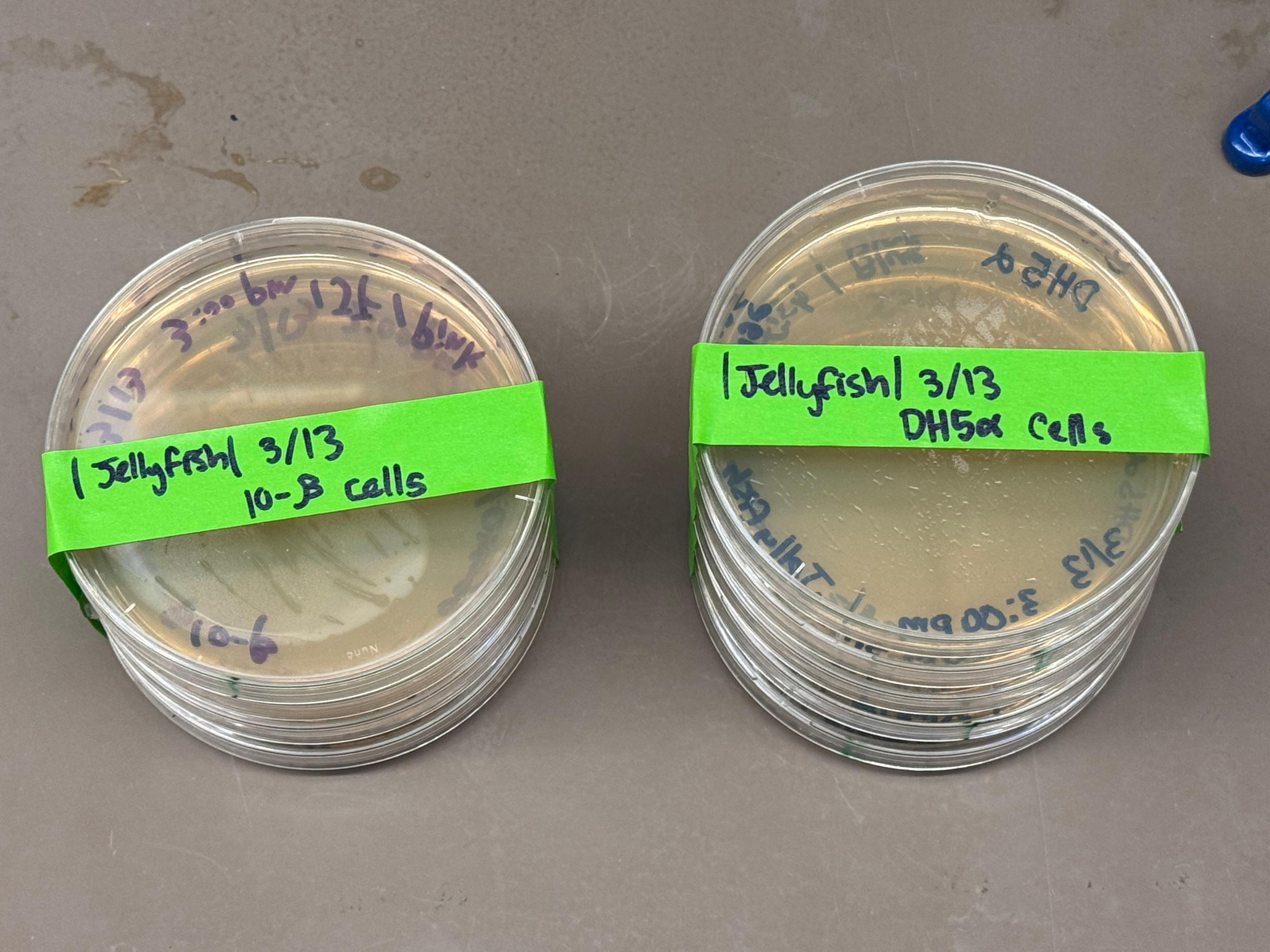
Results
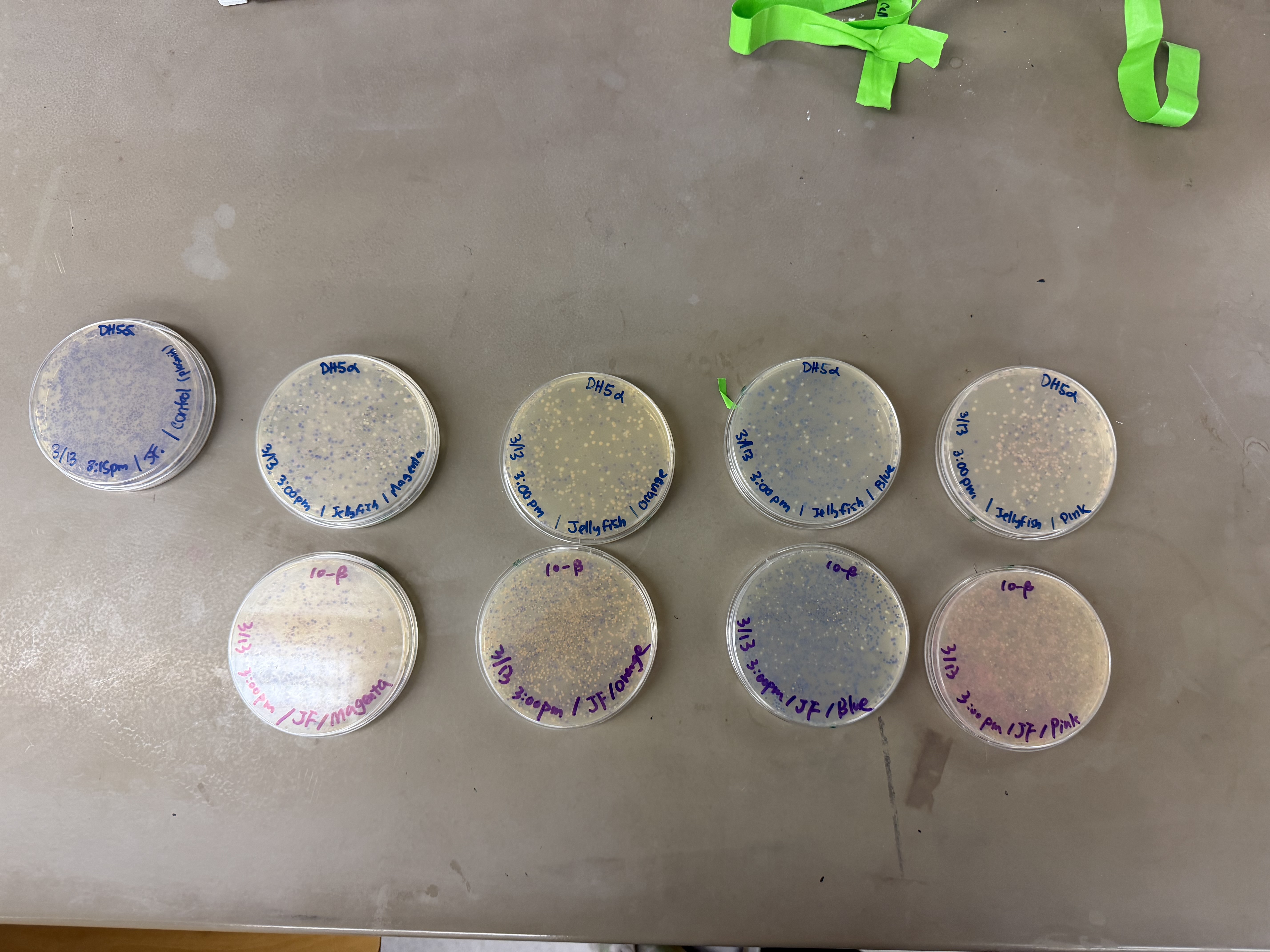
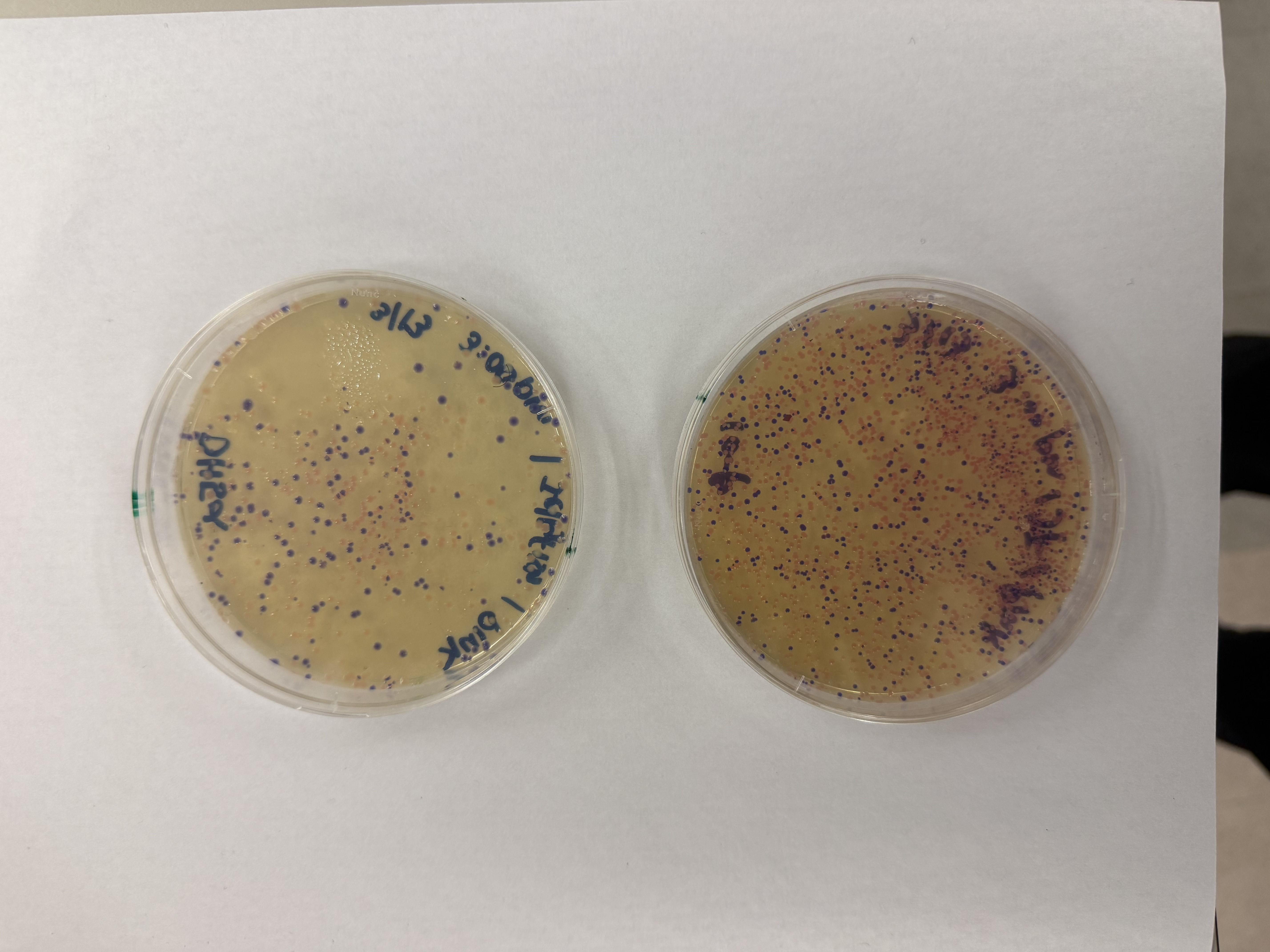
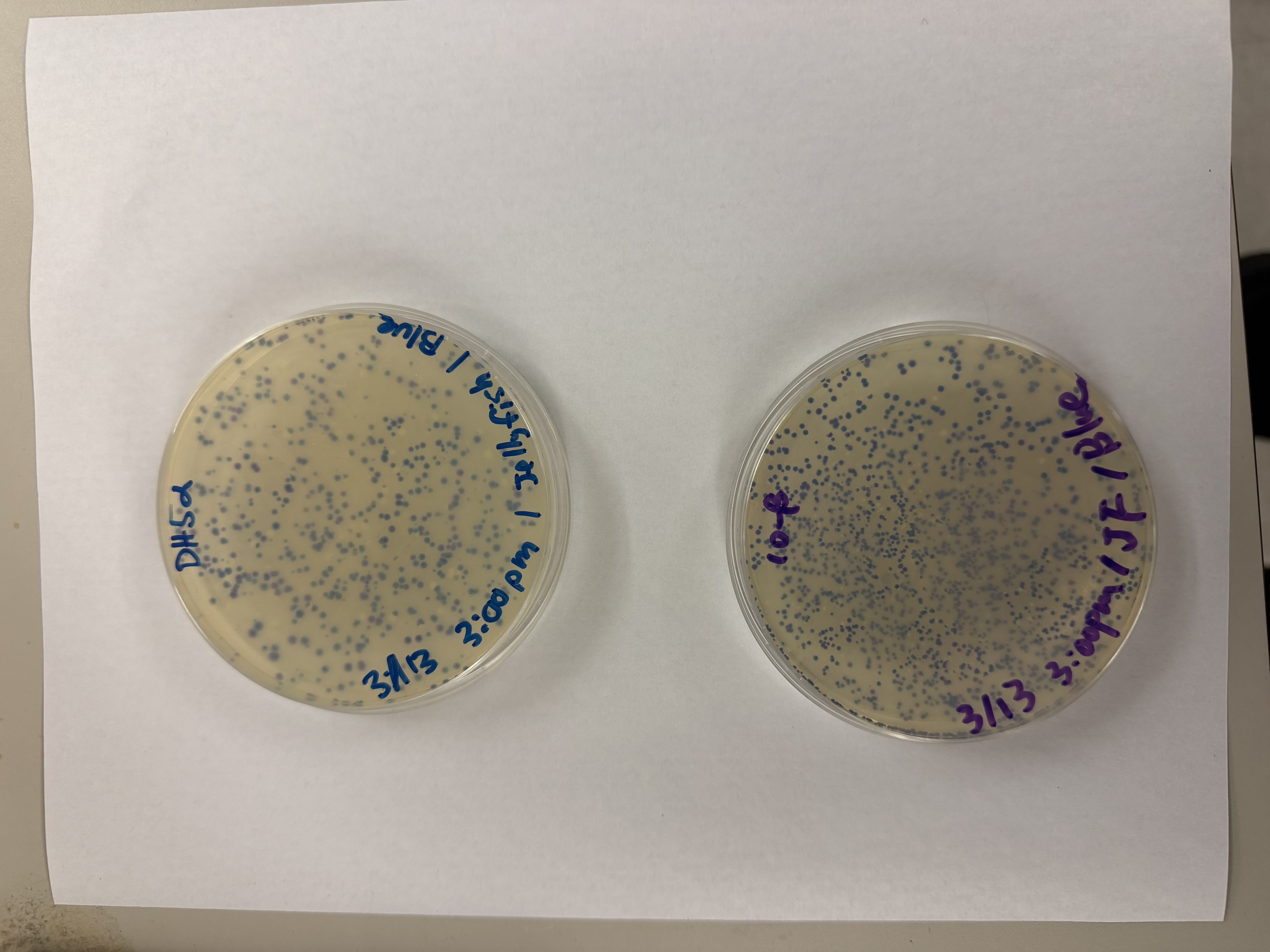
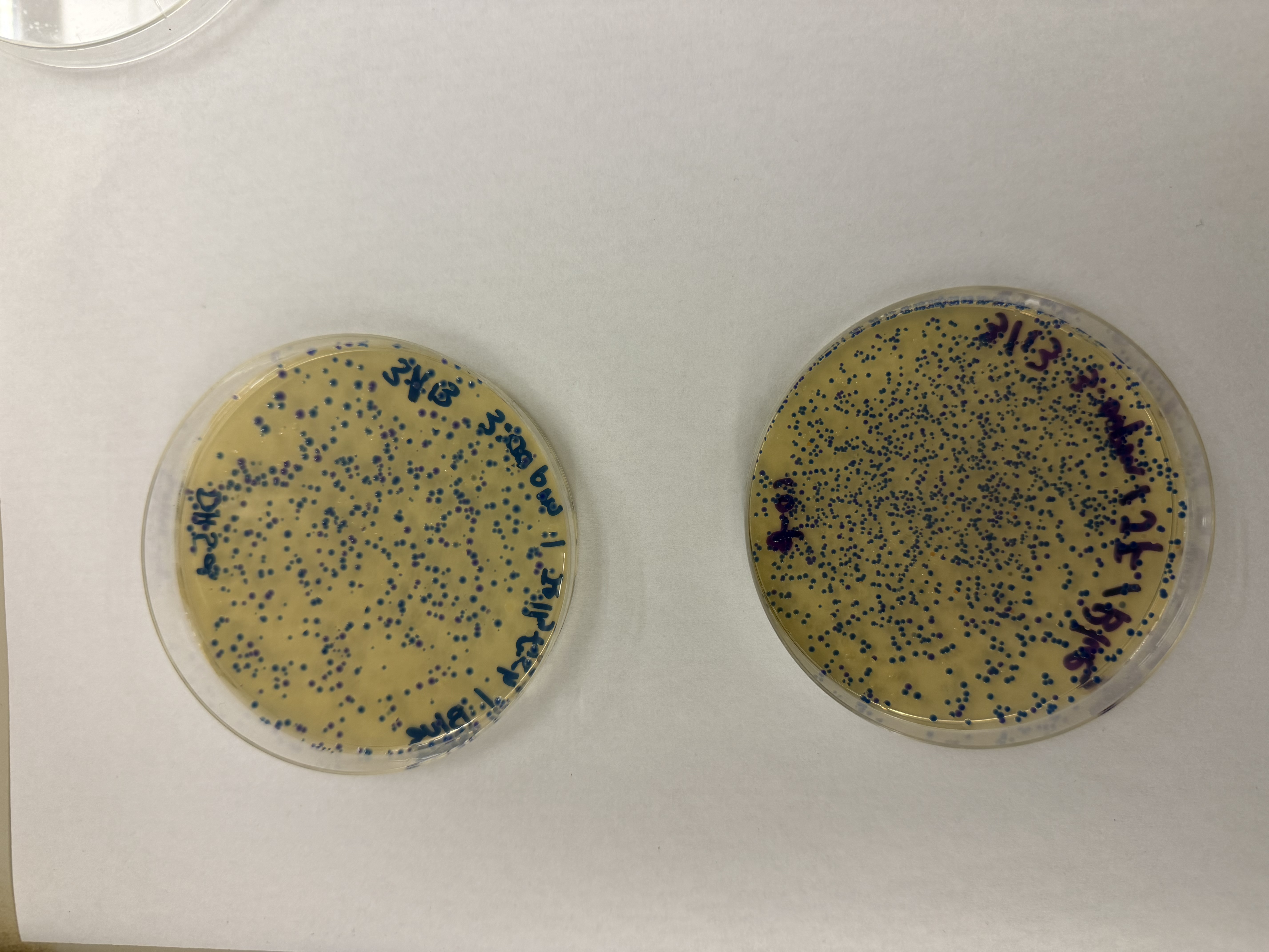
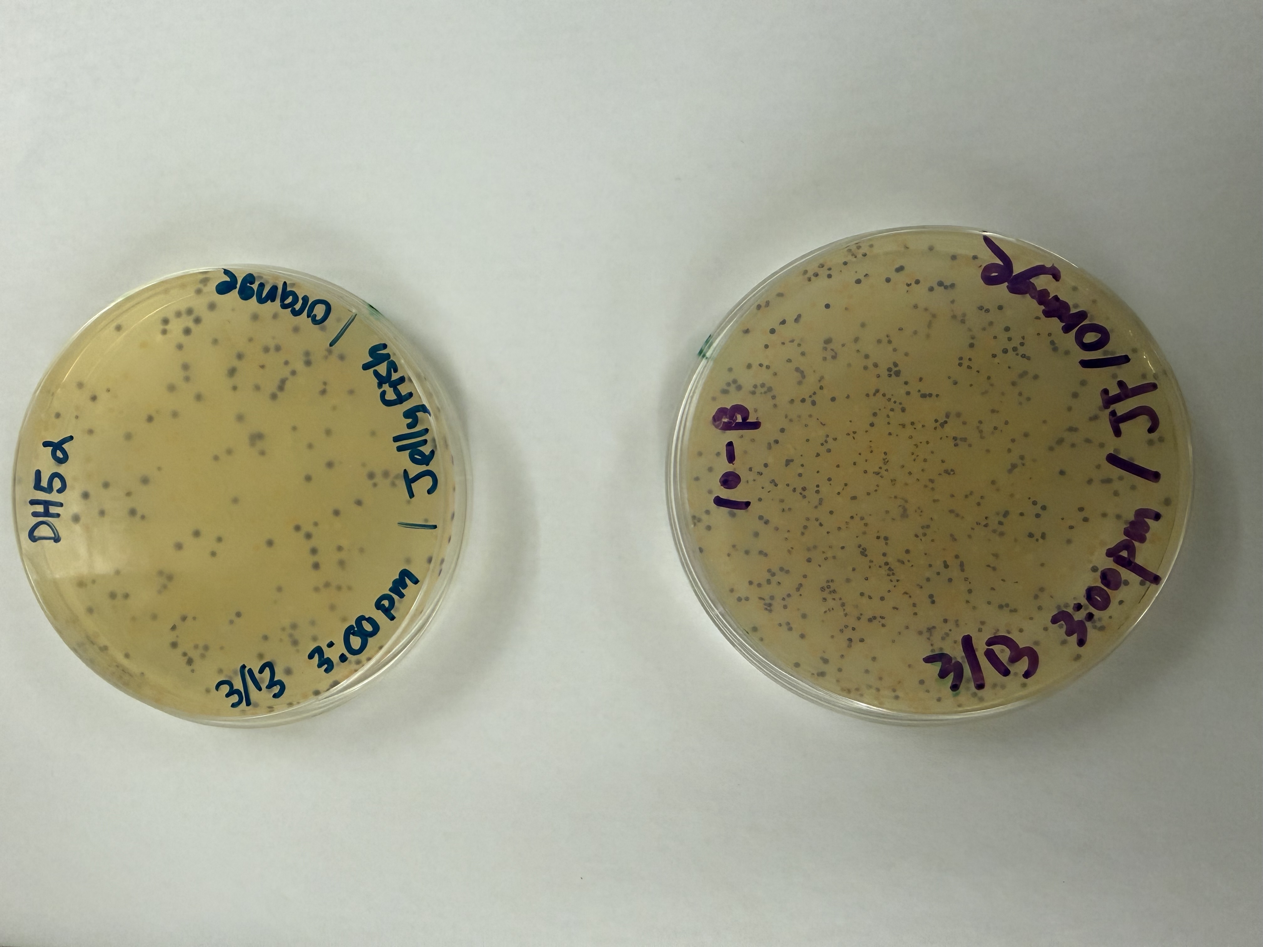
After 72 hours of incubation, the results were highly successful! We achieved the targeted chromophore mutations across both cell lines.
Analysis
The positive control confirmed the effectiveness of the assembly. While some purple colonies (native plasmid) were present on all plates, each plate showed distinct colored colonies (Orange, Pink, Blue, Magenta), indicating successful Gibson Assembly and transformation.
Control
Pink
Blue
Orange
Magenta
Gemini AI was consulted for formatting and content organization
Week 7 Lab: Neuromorphic Circuits
Intracellular Artificial Neural Networks (IANNs)
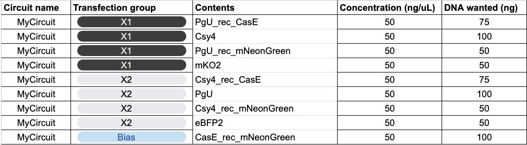
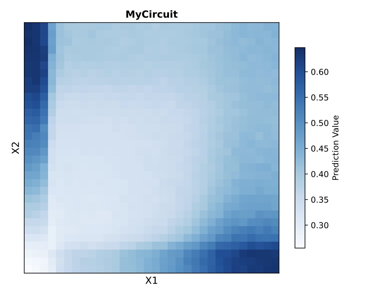
In this two-day lab, we designed and built our very own IANN using a library of plasmids from the Ron Weiss lab and human embryonic kidney (HEK) 293 cells. IANNs differ from traditional synthetic genetic circuits because IANNs can perform analog computations, rather than being limited to digital computations. IANNs are also universal function approximators—given an adequate number of intracellular artificial neurons, you can use an IANN to achieve any input/output behavior you’d like.
Day 1
I worked with a group of three, and this was the circuit we designed:
Here are the predicted results by the biocompiler:
Day 2
On day 2, we took a trip to the Weiss Lab and Evan started the protocol on the Opentrons machine to begin construction of our neuromorphic circuits. We also looked at some immortalized human cells on a microscope, giving insight to experimental mammalian cell biology.
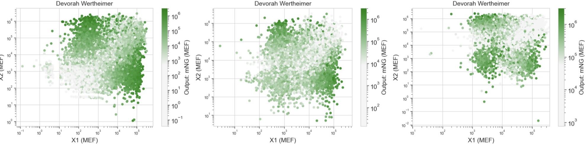
Results
Our results didn’t quite match the prediction. This is due to the fact that our uploaded circuit violated some of the “laws” governing the system’s design (we learned this later), but the computer still allowed these “illegal” circuits to be generated and simulated.
Gemini AI was consulted for formatting and content organization
Week 9 Lab: Protein Purification & Mycelium
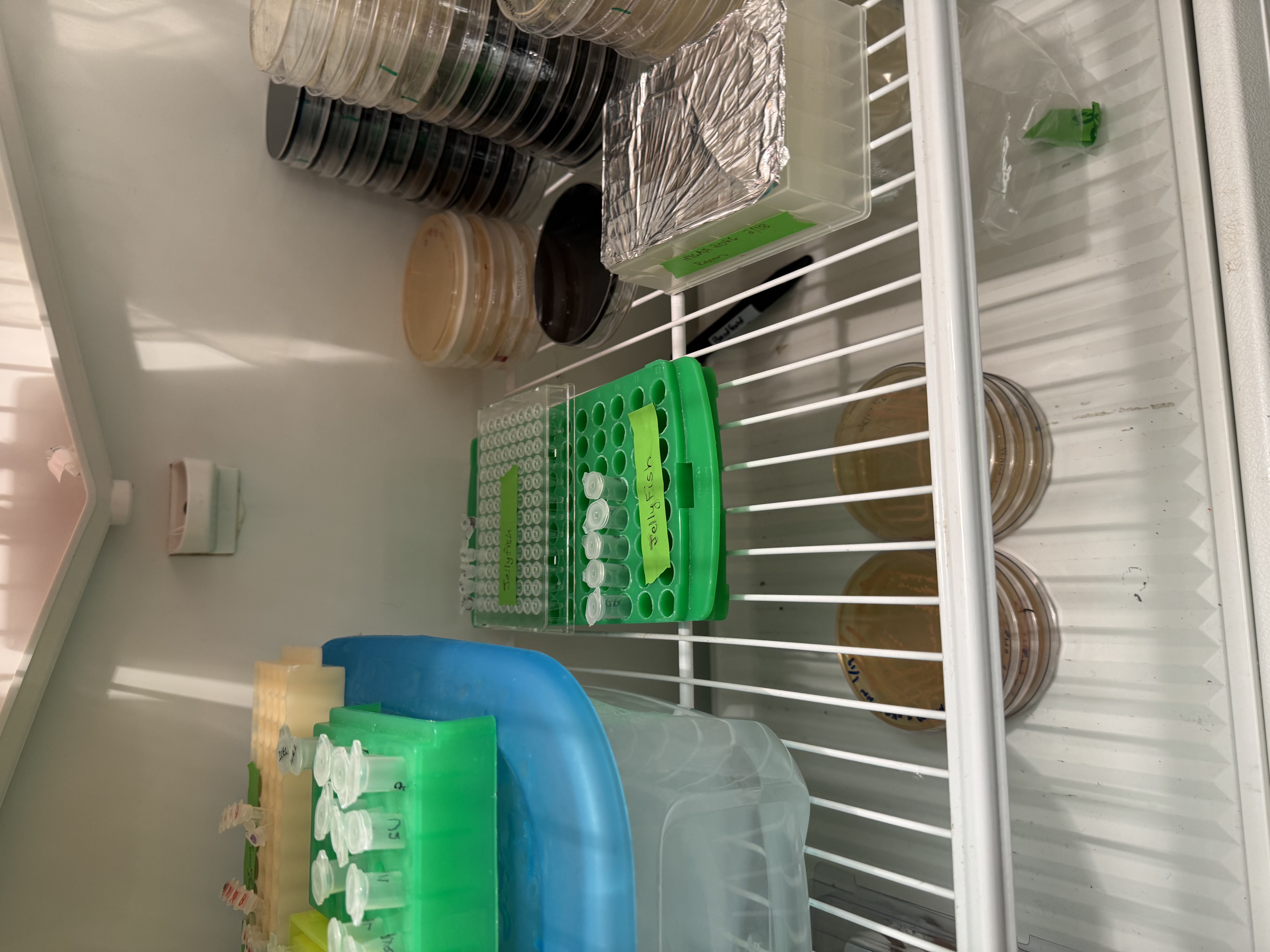
Fungal Materials Follow-up
The first thing we did was look at our mycelium molds (no pun intended). We are tracking the growth and structural integrity of the fungal networks as they colonize the substrates.
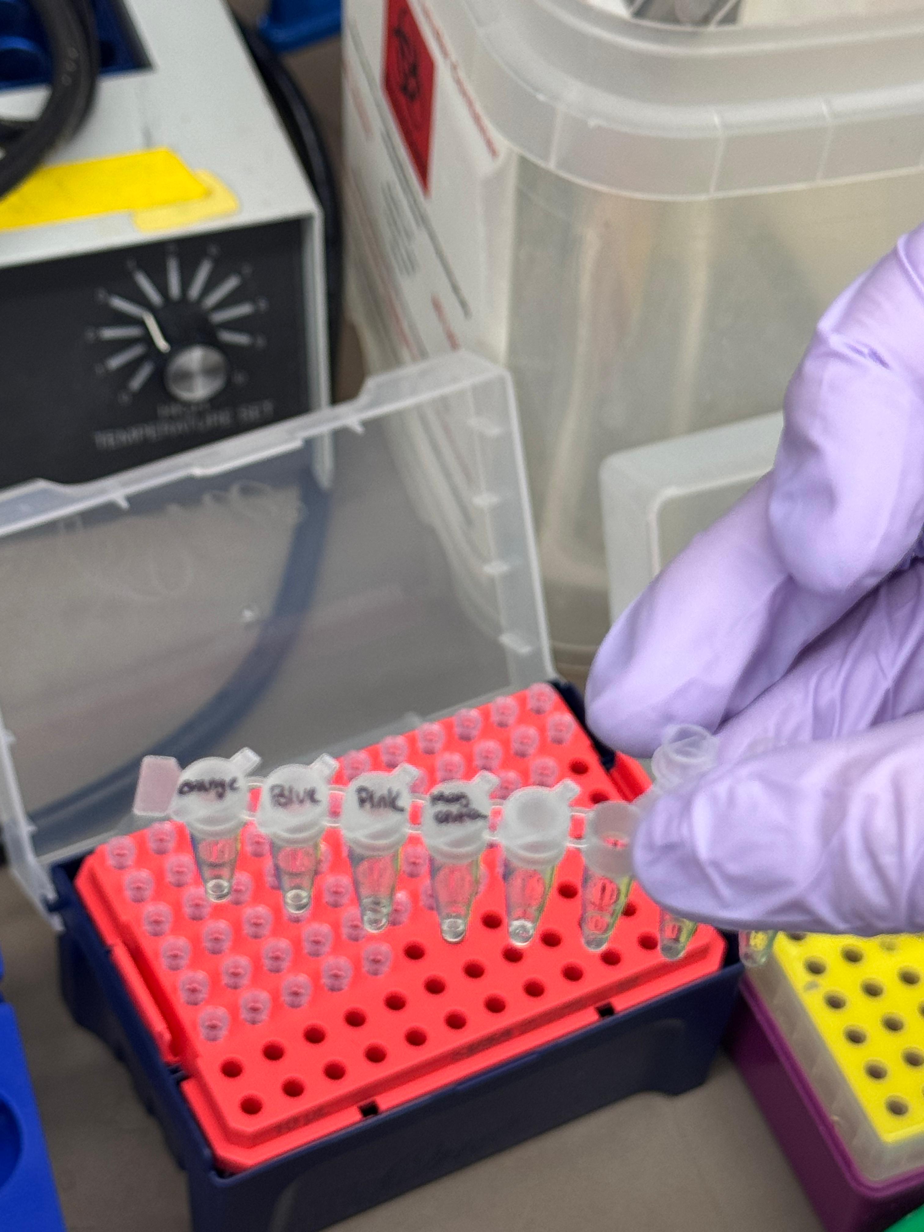
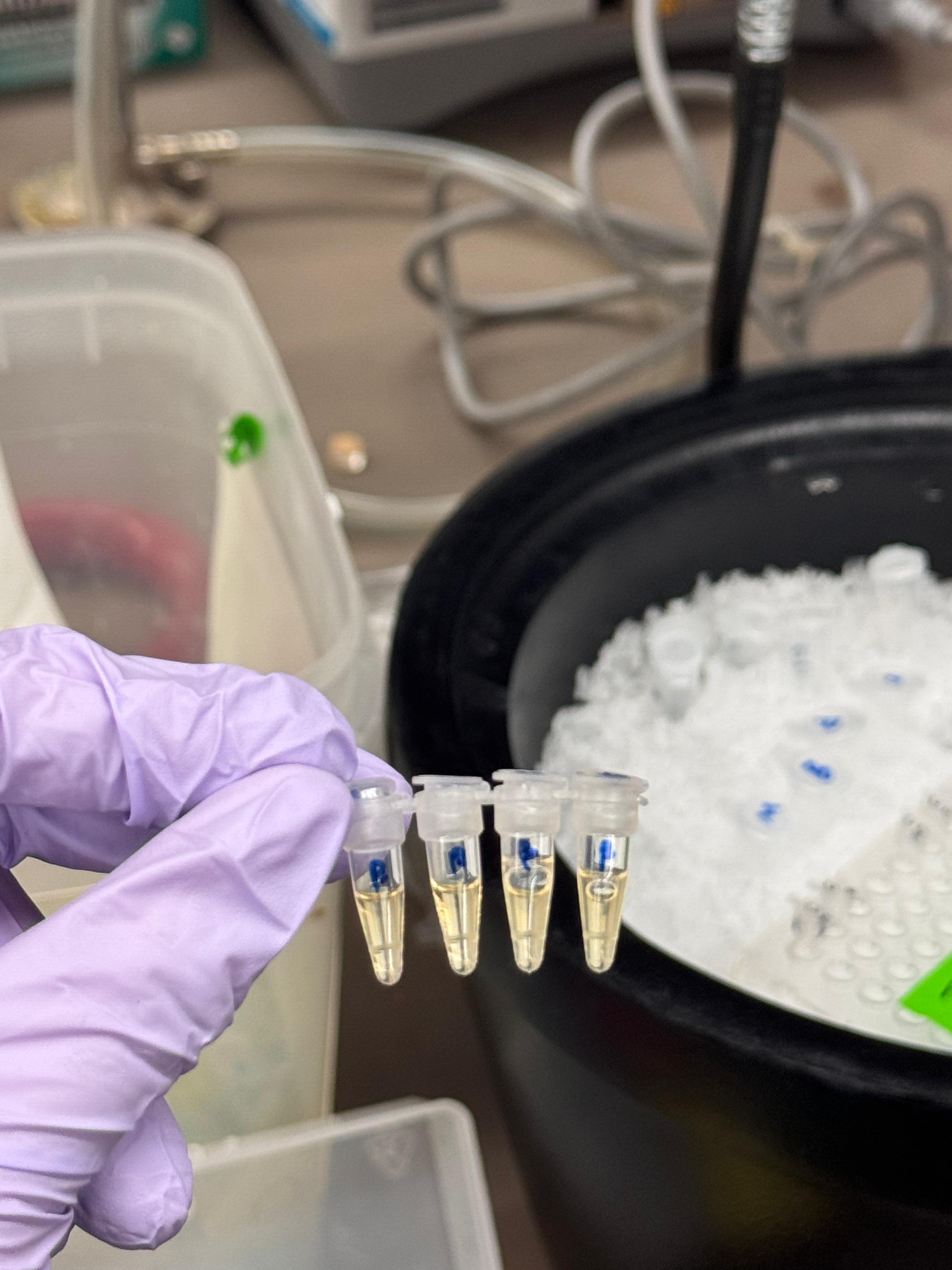
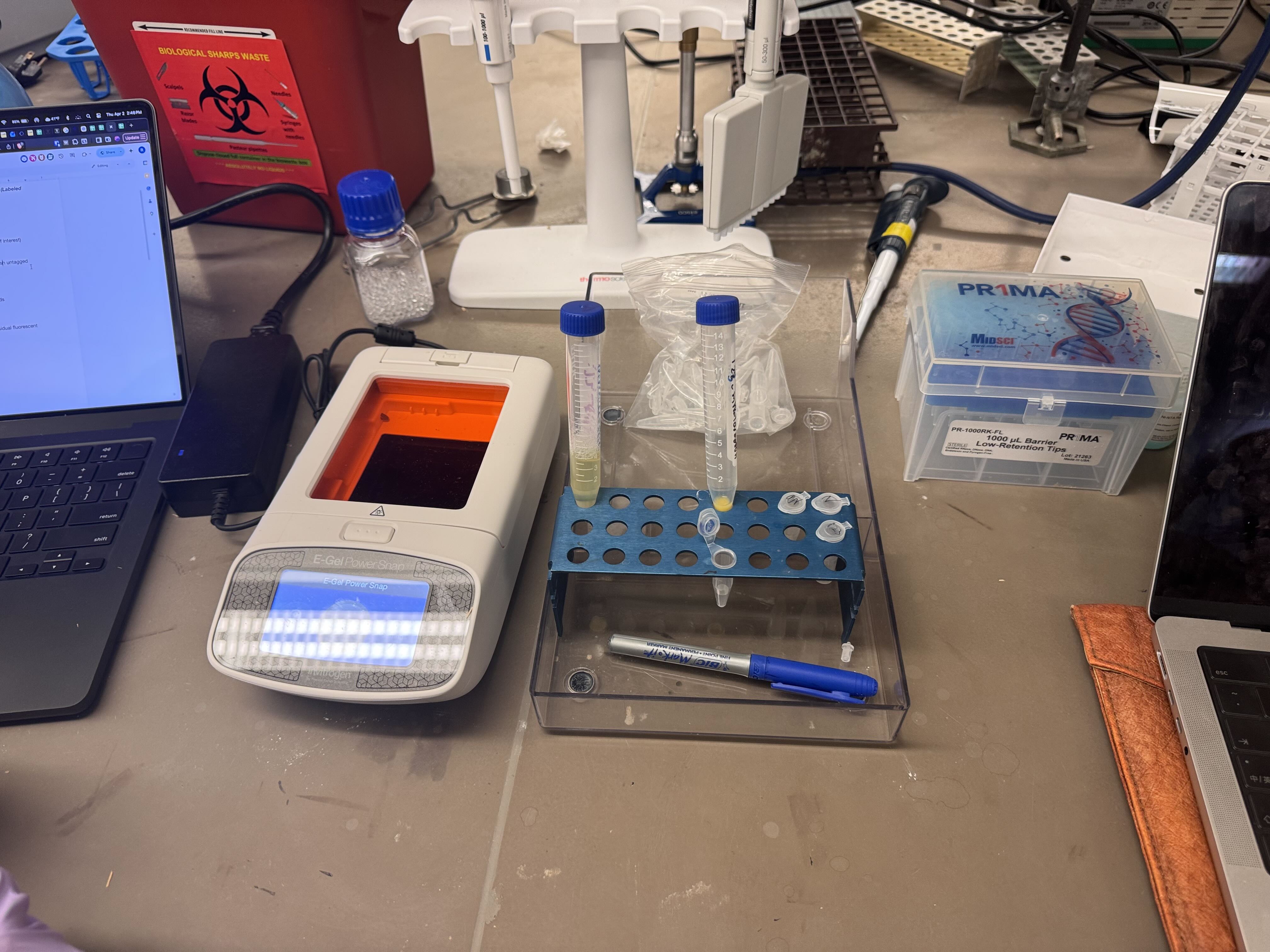
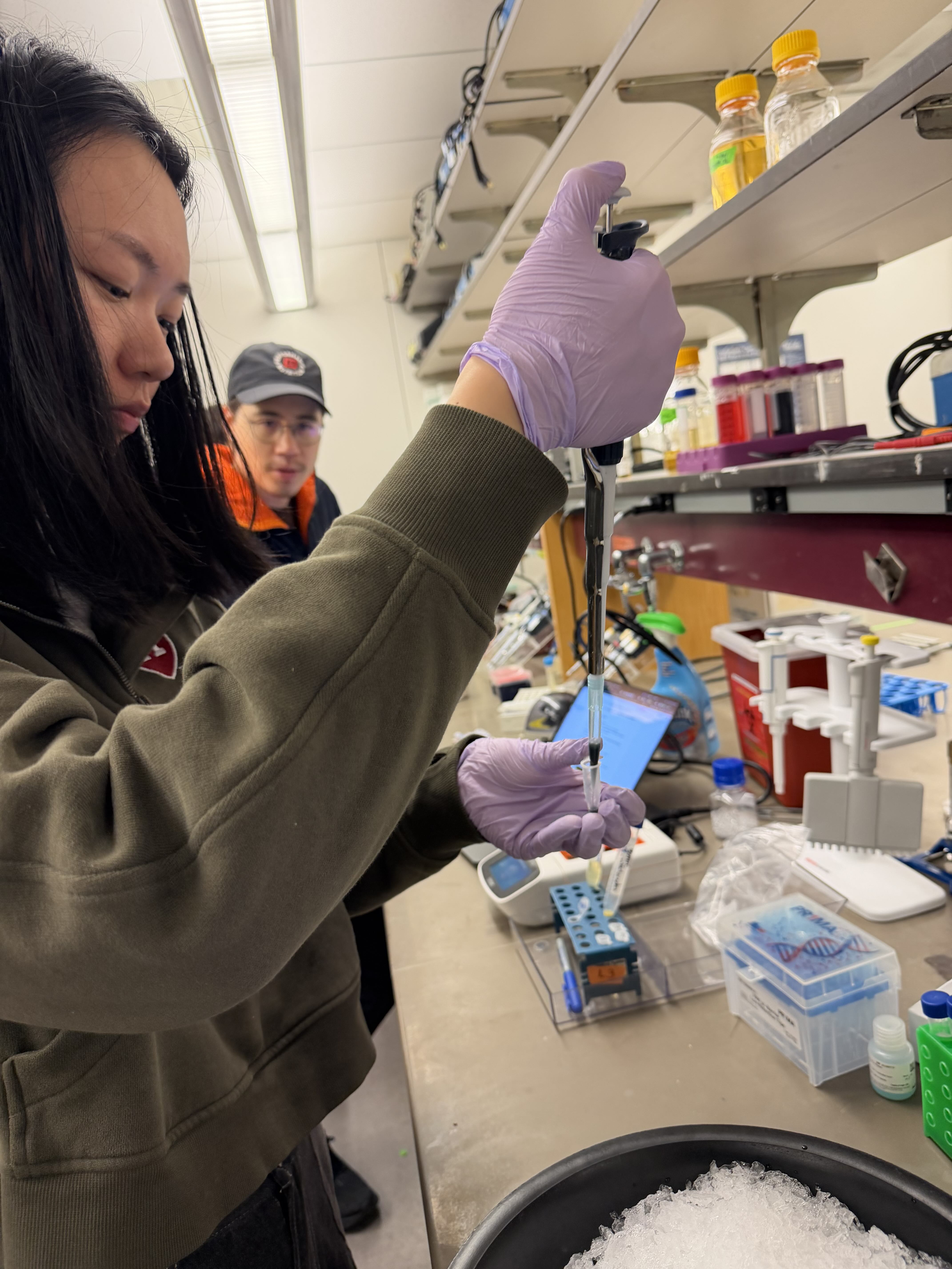
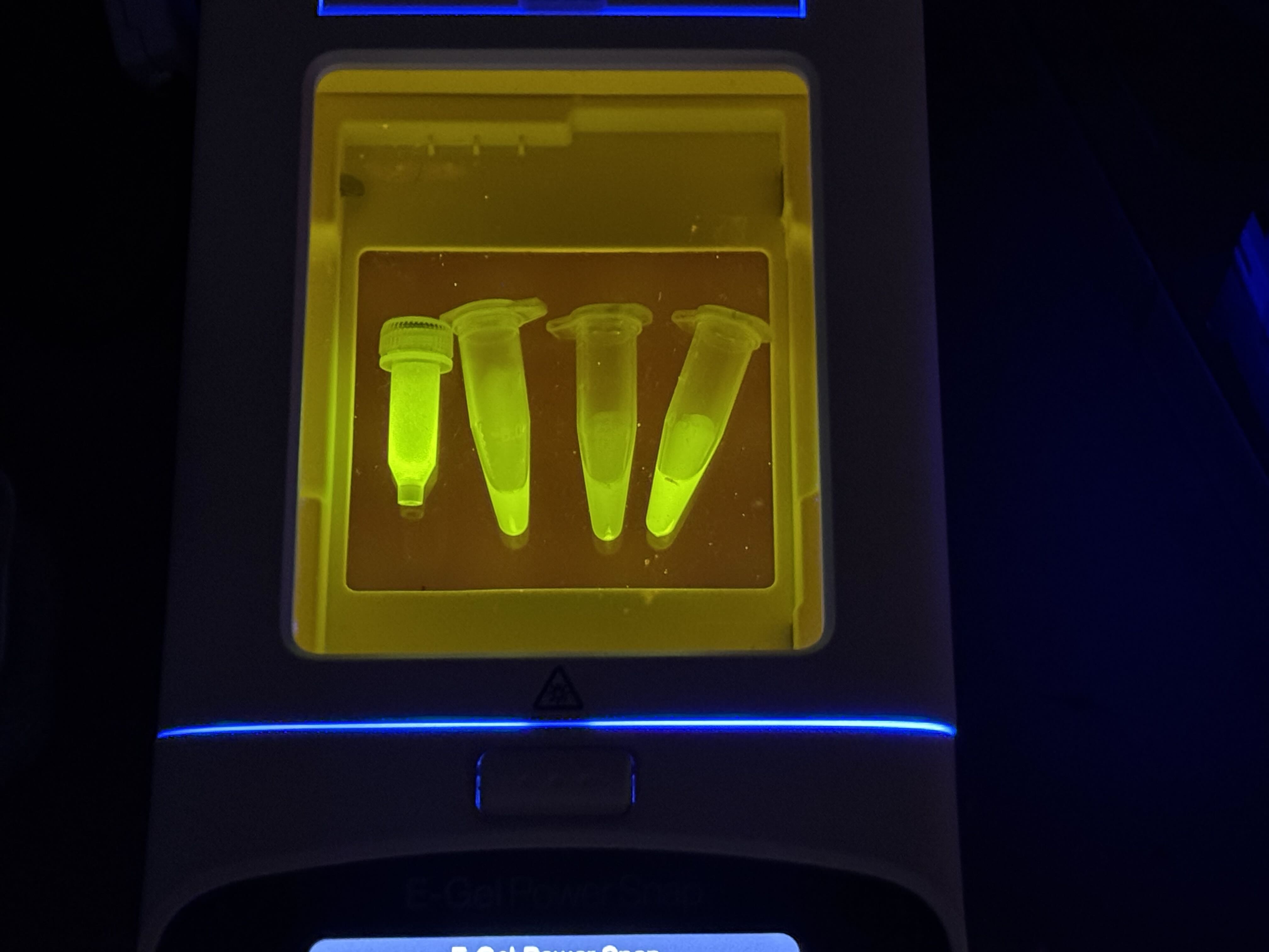
Protein Purification: An Introduction
To isolate our protein of interest, we first had to grow the cells and then lyse them using a combination of B-PER (Bacterial Protein Extraction Reagent) and sonication. This process breaks open the cell membranes, resulting in a lysate solution (labeled as Tube A) that contains the total protein content of the cells.
Method 1: Magnetic Bead Protein Purification
This method utilizes functionalized magnetic beads to “grab” tagged proteins out of the lysate.
The Procedure:
Binding: Added magnetic beads to the solution (labeled Tube B).
Separation: Took 500µL of the mWatermelon + mag beads and placed them onto a magnet tray. The beads (now bound to our protein of interest) sat tight against the magnet.
Clearing: Pipetted out the residual volume (excess proteins and buffer).
Washing: Added 500µL of Wash Buffer (containing a small amount of imidazole, 20mM) to wash any untagged, non-specific proteins from the beads. Mixed well and returned to the magnet tray to remove the wash.
Elution: Added 200µL of Elution Buffer (containing a high concentration of imidazole, 500mM) to strip the protein from the beads.
Collection: After the beads settled on the tray, we pipetted the liquid out. This is Solution 4.
Repeat: Repeated the elution step with another 200µL of Elution Buffer to catch any residual fluorescent protein. This resulted in Solution 5, which still contained a significant amount of FPs.
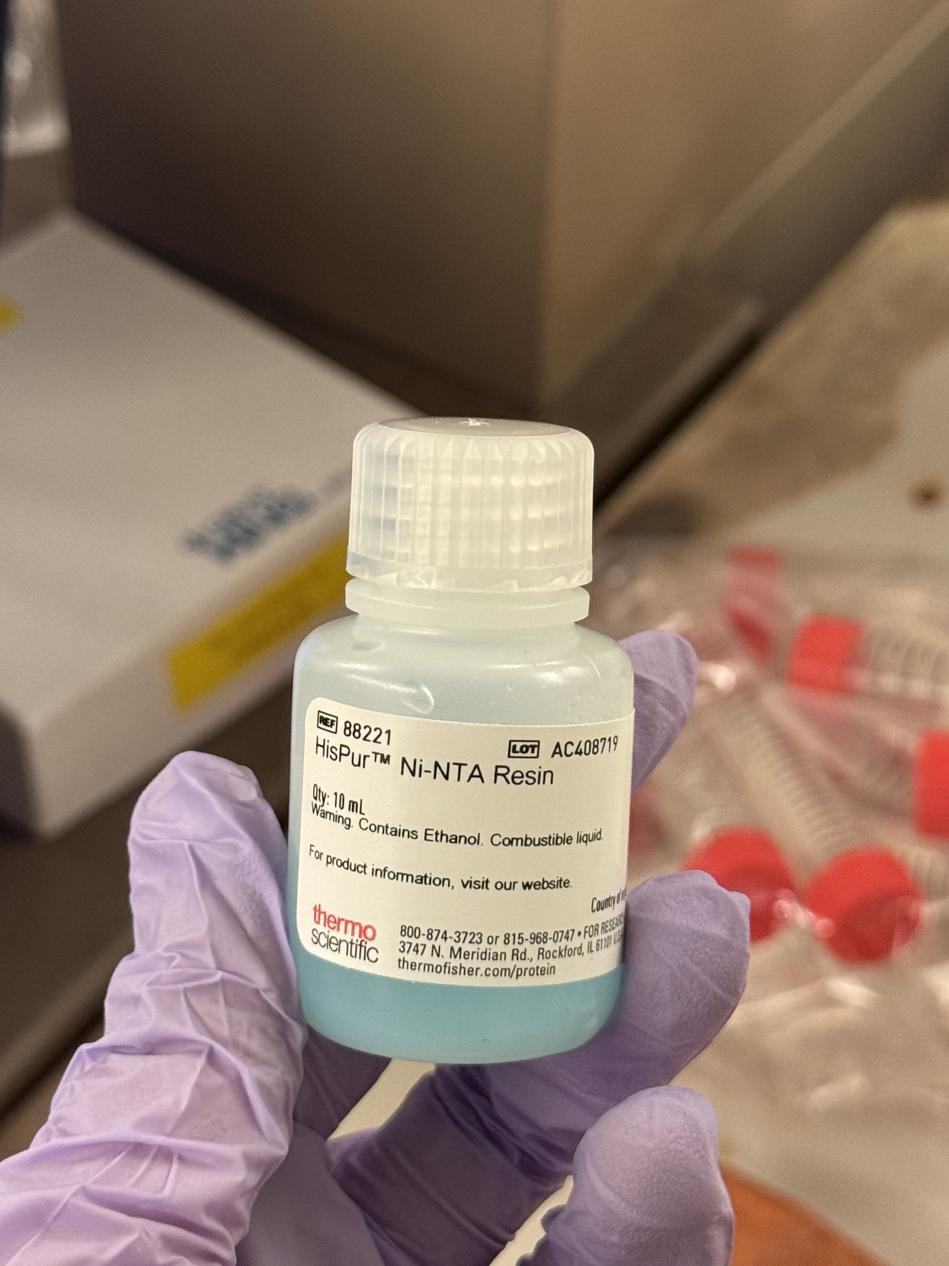
Method 2: Ni-NTA Spin Column Protein Purification
As an alternative to magnetic beads, we used Ni-NTA (Nickel-Nitrilotriacetic acid) beads in a spin column format, which relies on centrifugal force to move the buffers through the resin.
The Procedure:
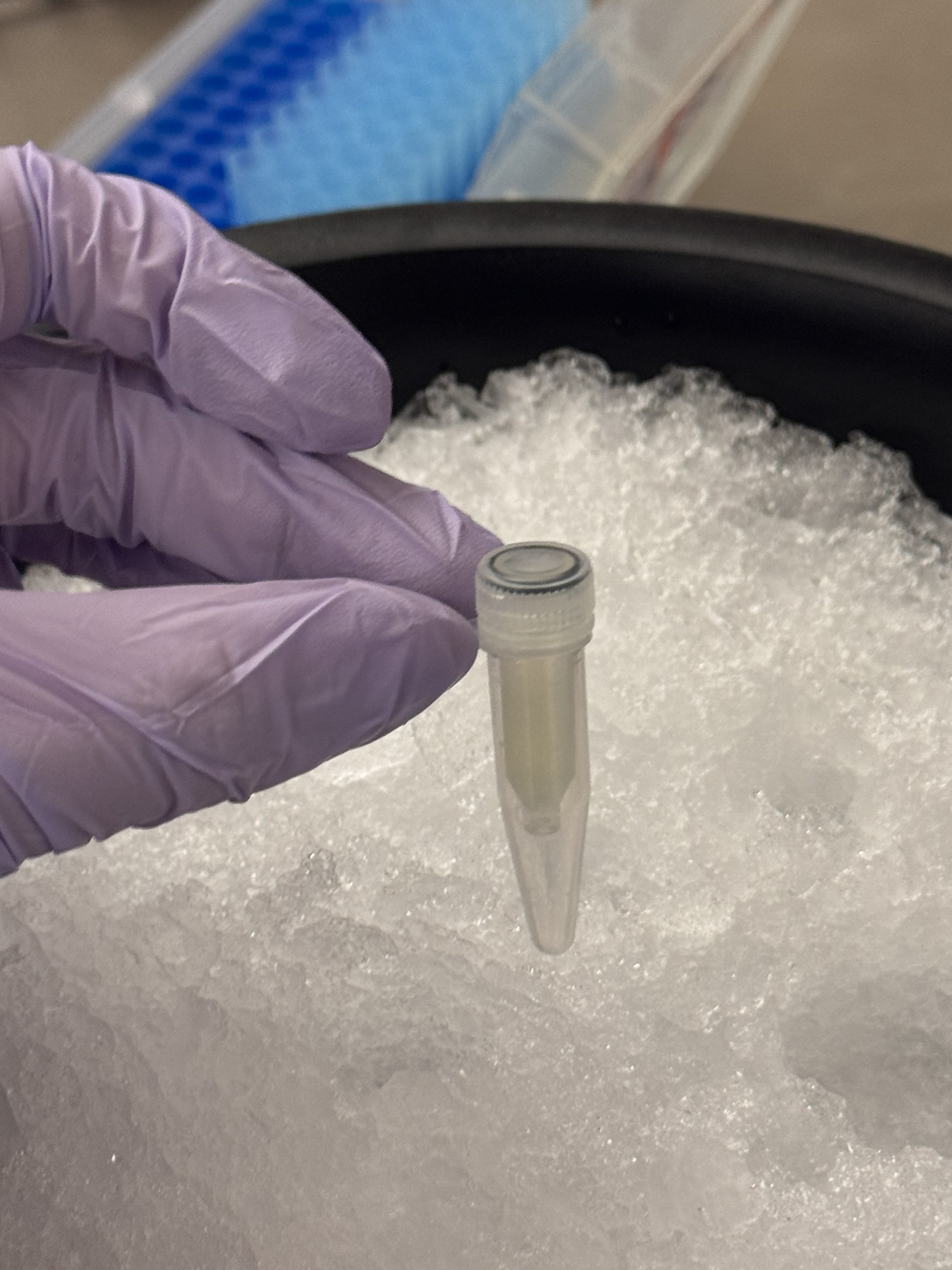
Incubation: Combined 200µL of Ni-NTA bead solution with 2mL of lysate. We let this incubate for 30 minutes to allow the His-tagged proteins to bind to the nickel resin.
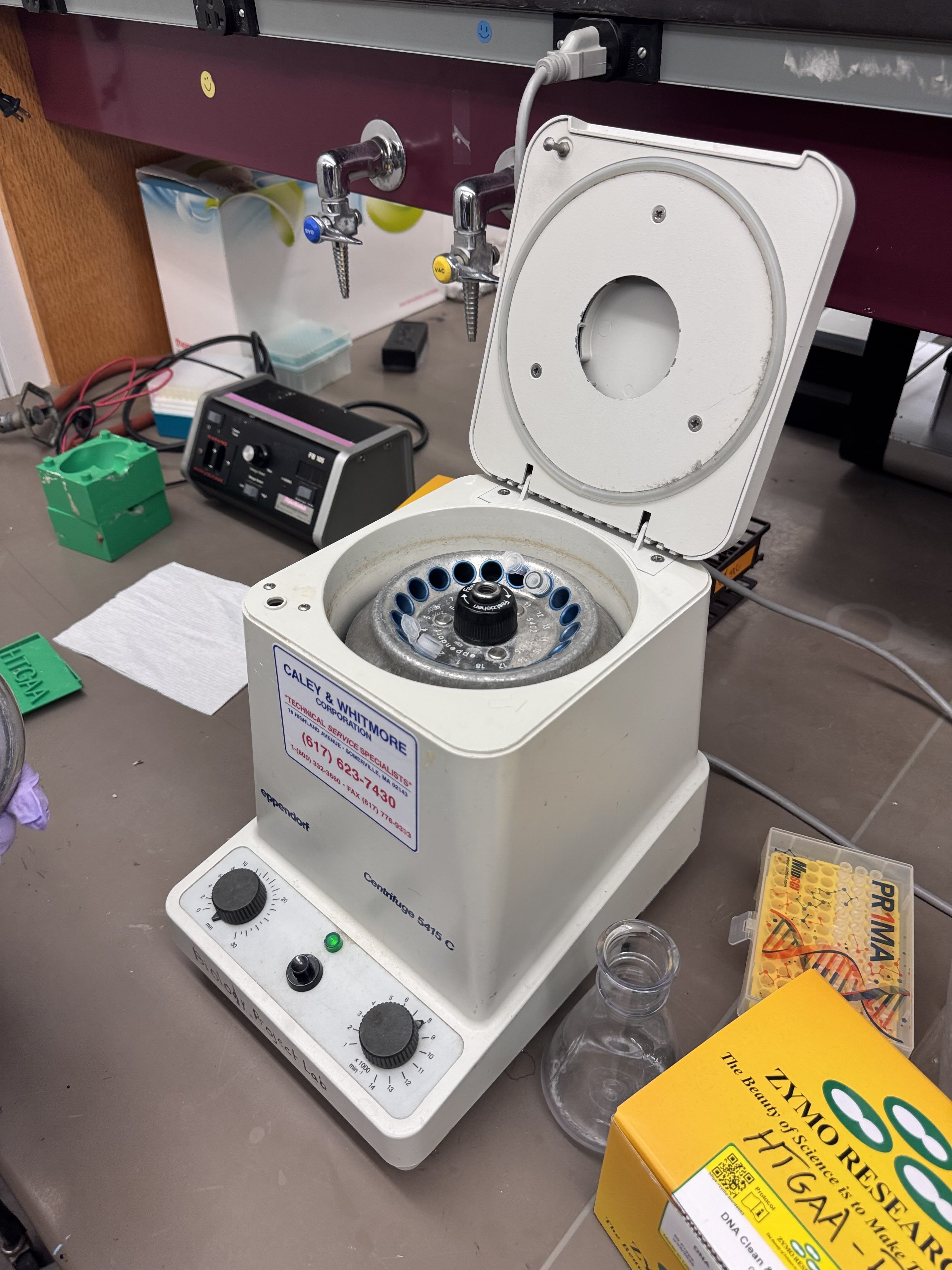
Binding Spin: Transferred to an eppy tube and spun at 8,000 RPM for 1 minute. We collected and observed the flow-through.
Wash Step: Added 500µL of wash buffer to the column and spun again at 8,000 RPM for 1 minute.
Elution: Added 200µL of Elution buffer and performed a final spin at 8,000 RPM for 1 minute.
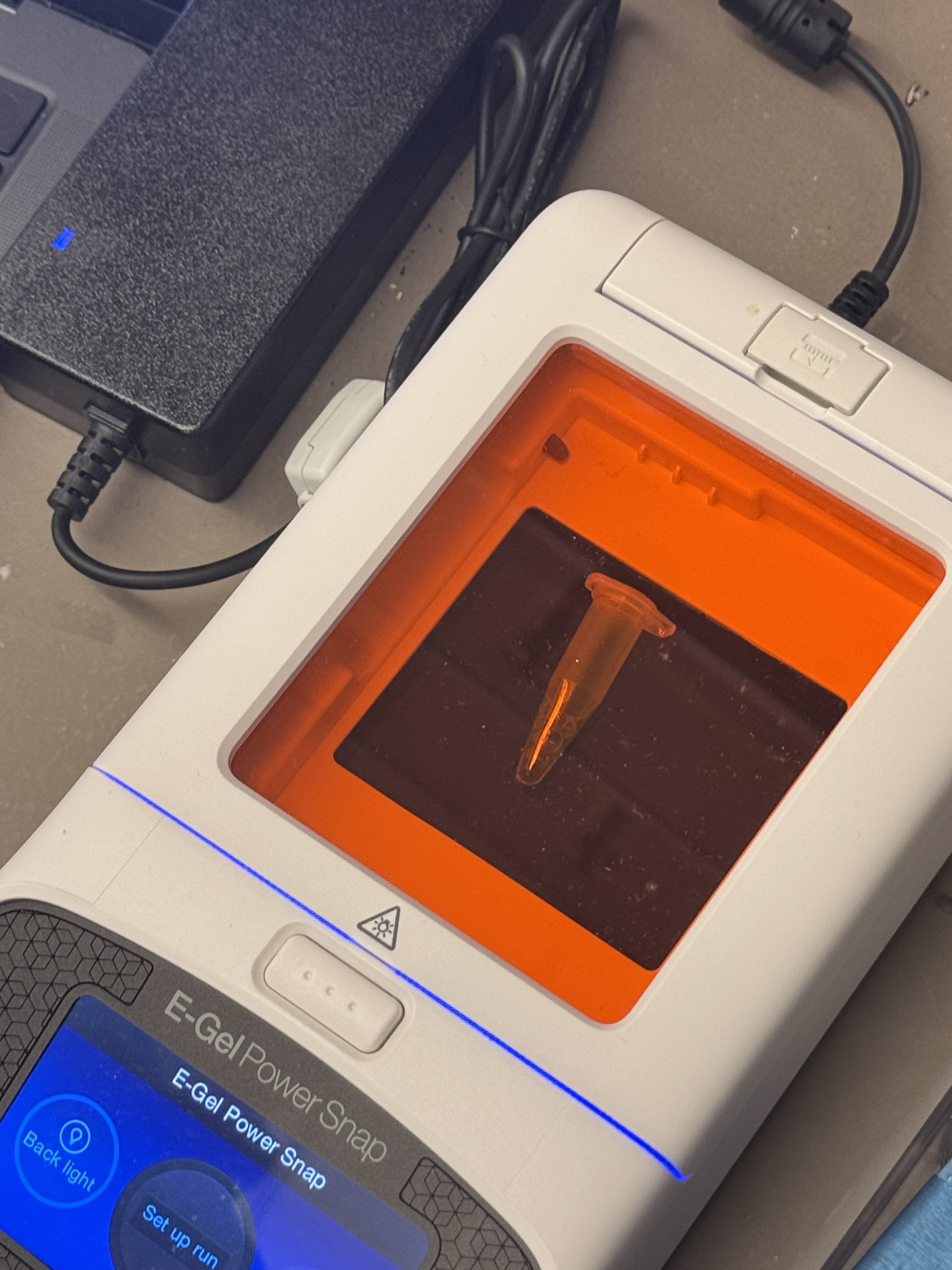
Observation: We analyzed the final flow-through to confirm the presence of our purified protein.
Gemini AI was consulted for formatting and content organization