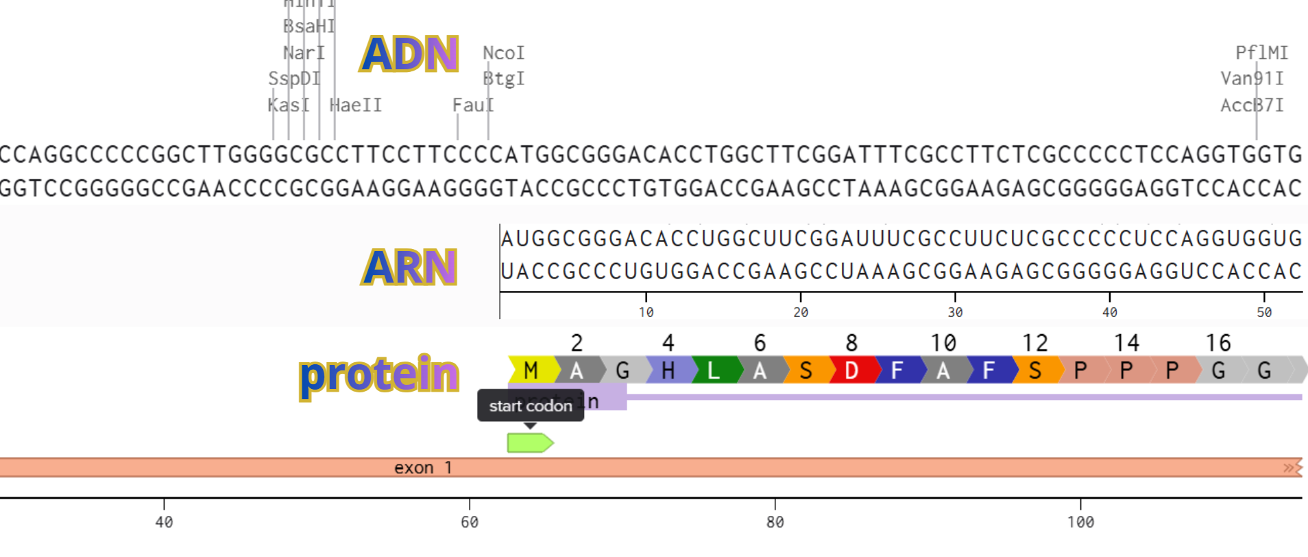
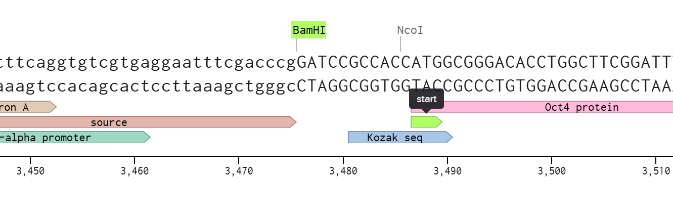
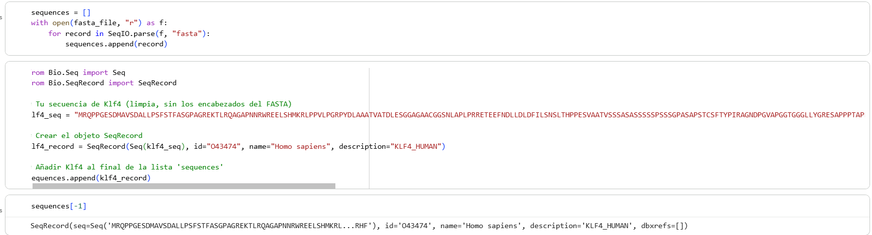
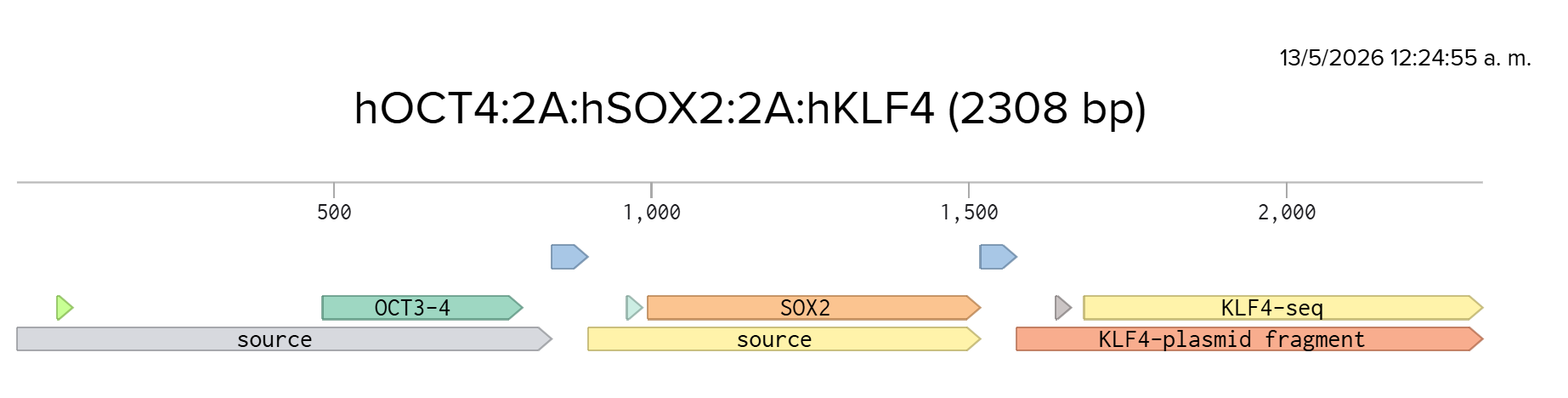
First I retrieved the sequence of the yamanaka factors from Addgene:
Oct3/4 (https://www.addgene.org/13366/) #13366
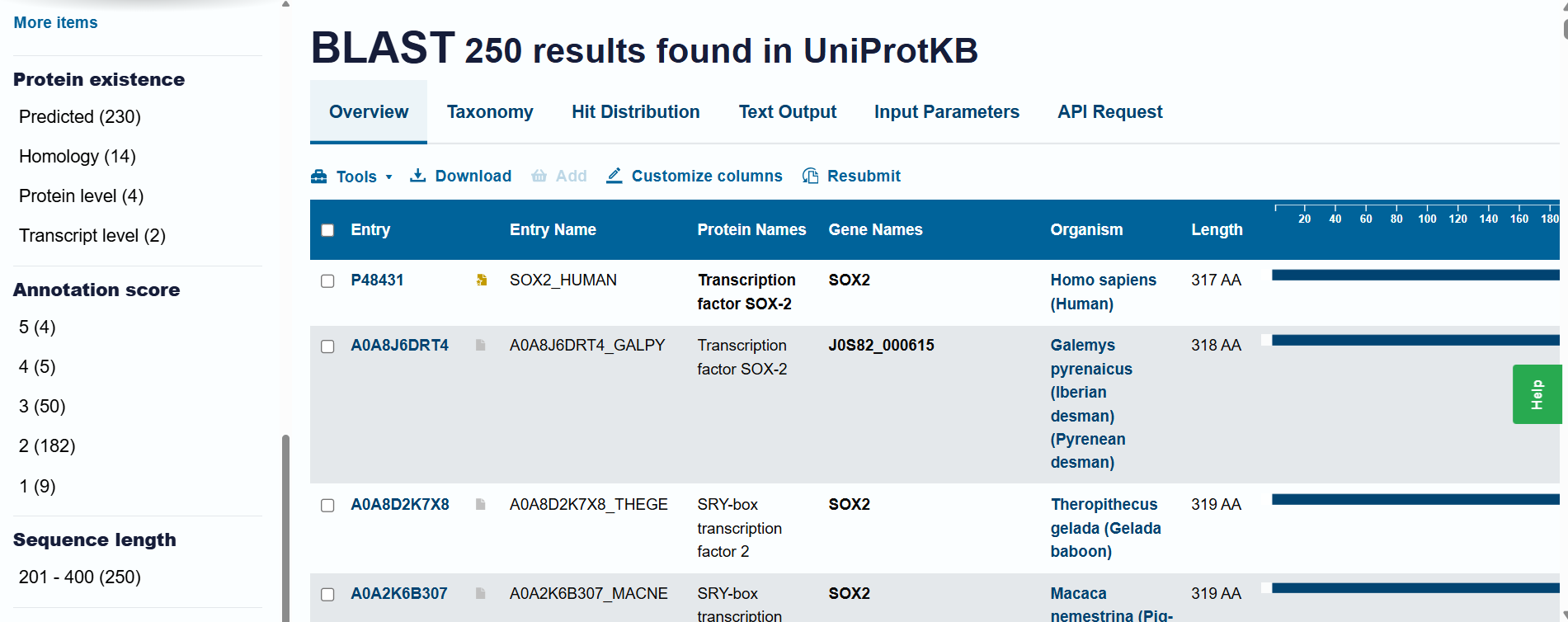
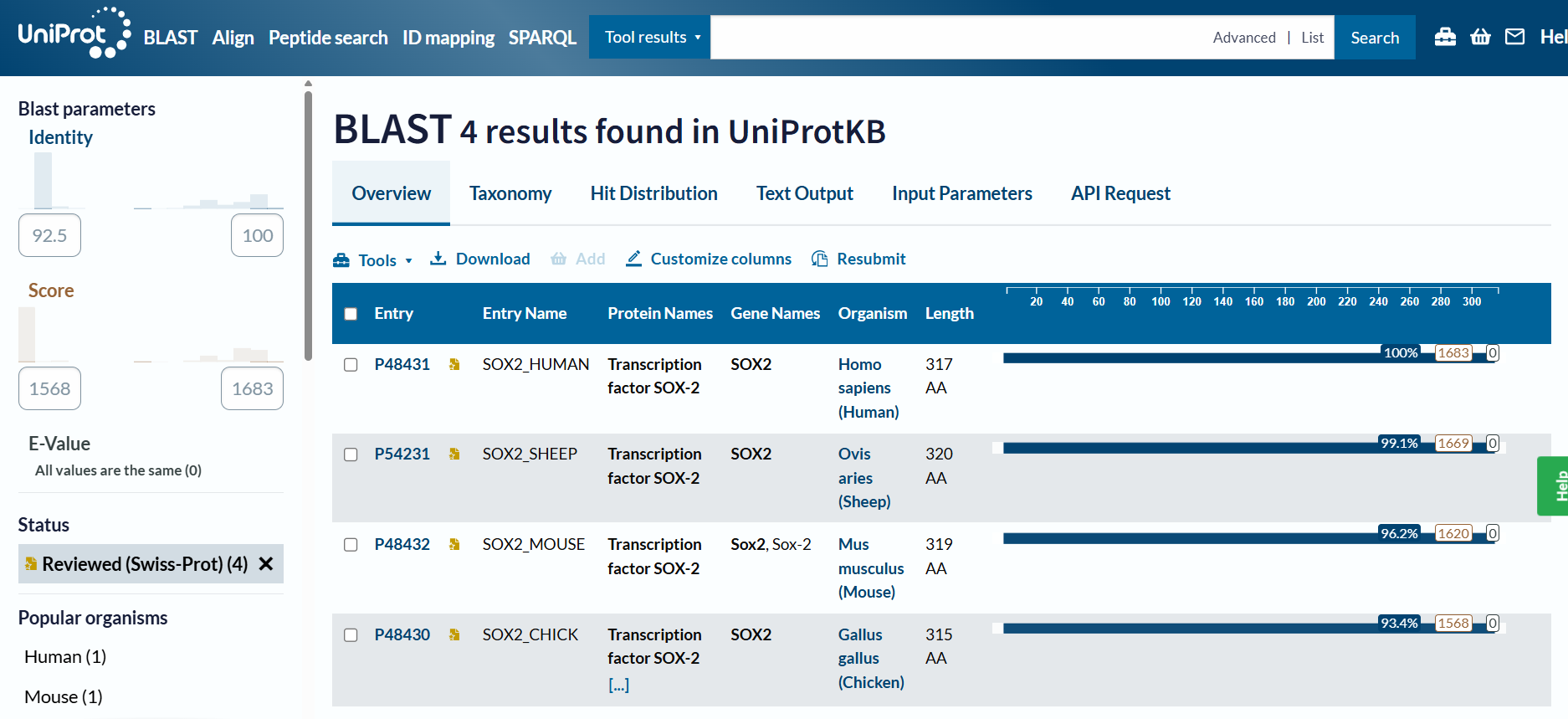
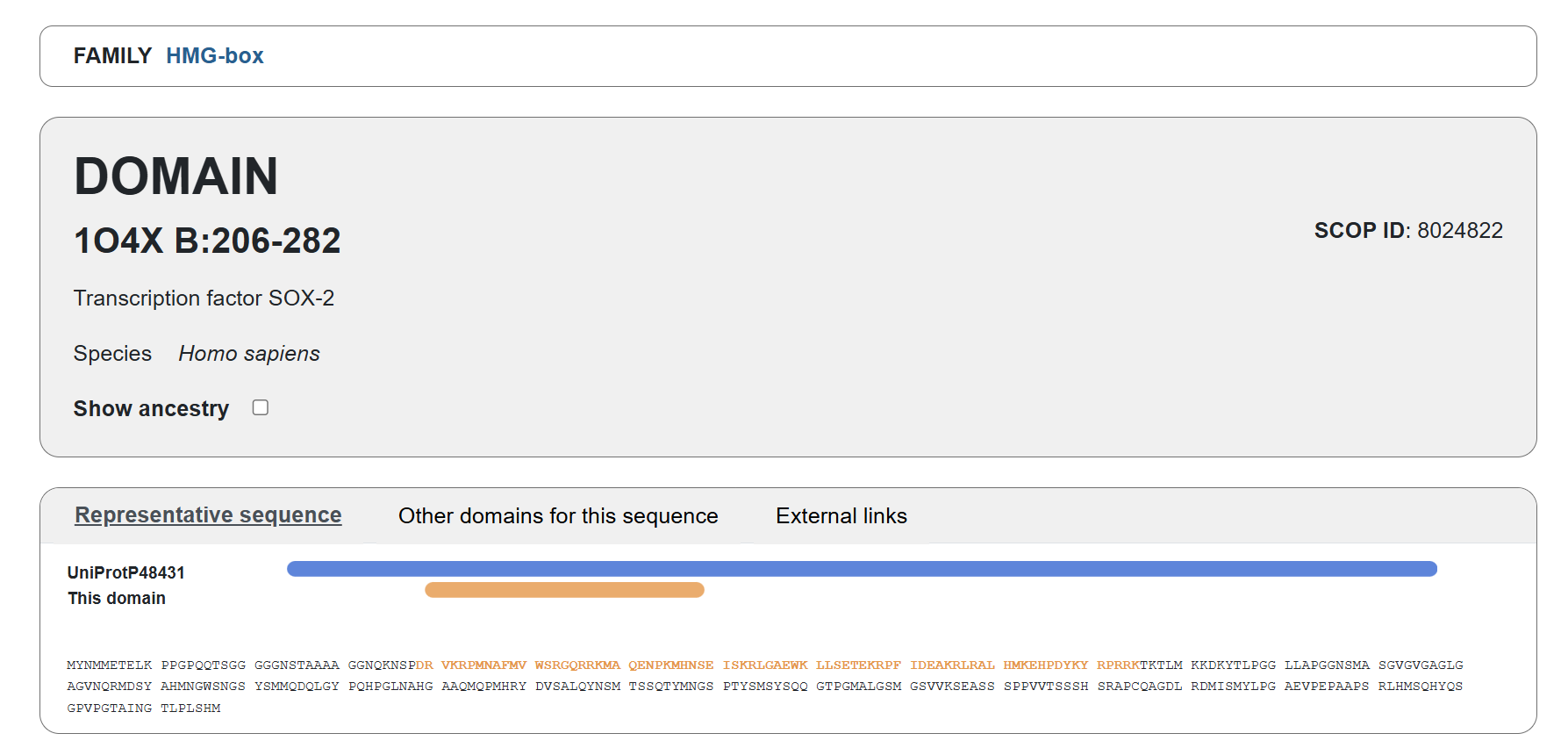
Sox2 (https://www.addgene.org/13367/) #13367
Klf4 (https://www.addgene.org/13370/) #13370
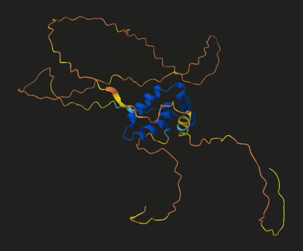
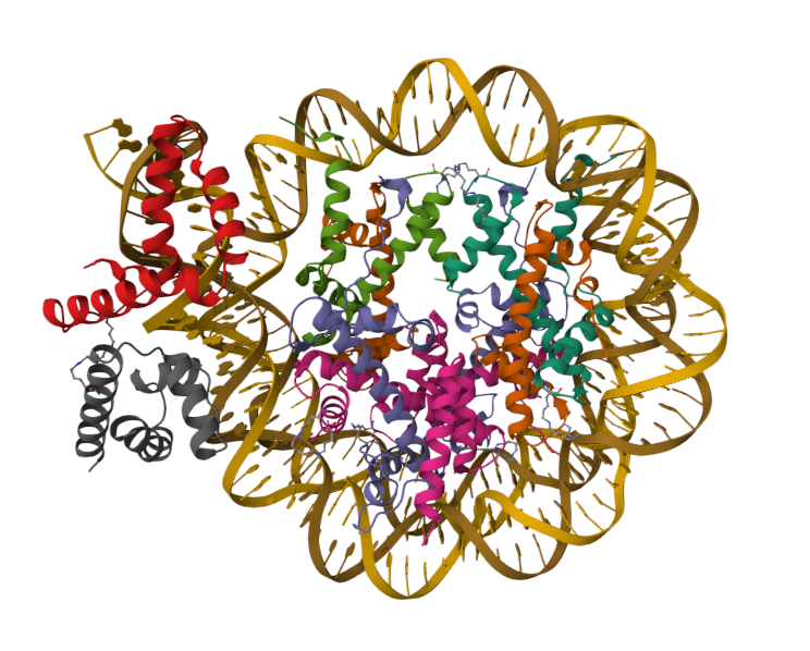
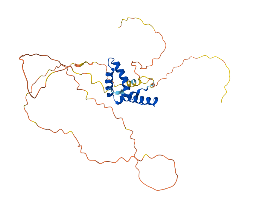
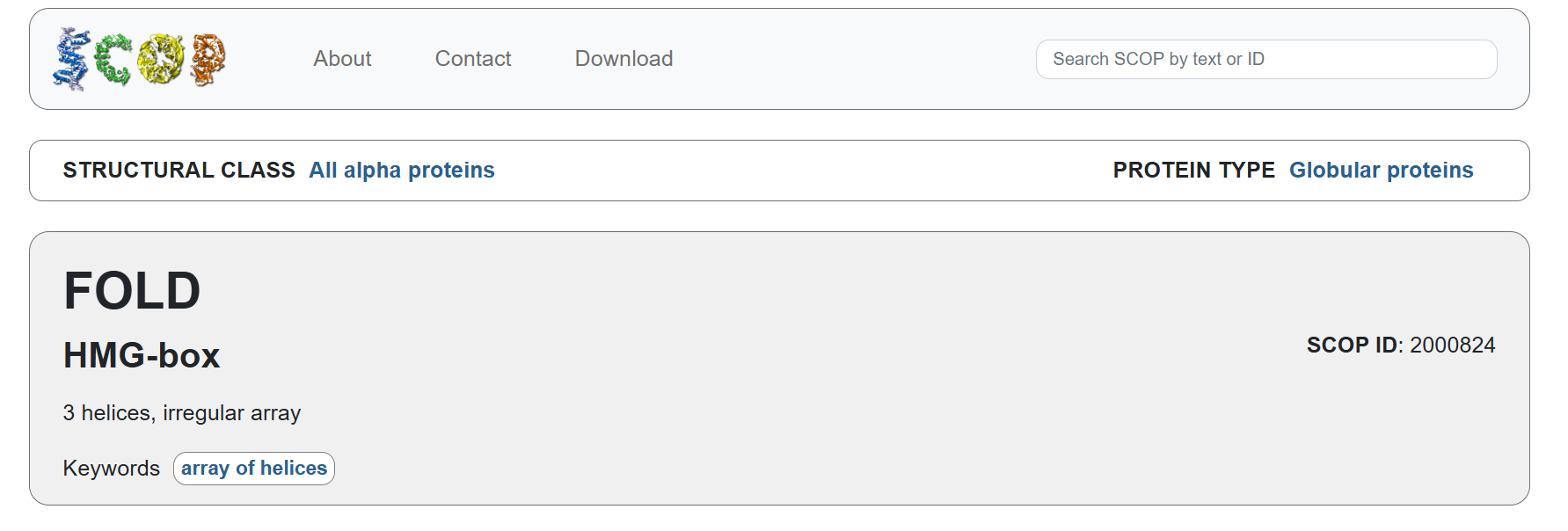
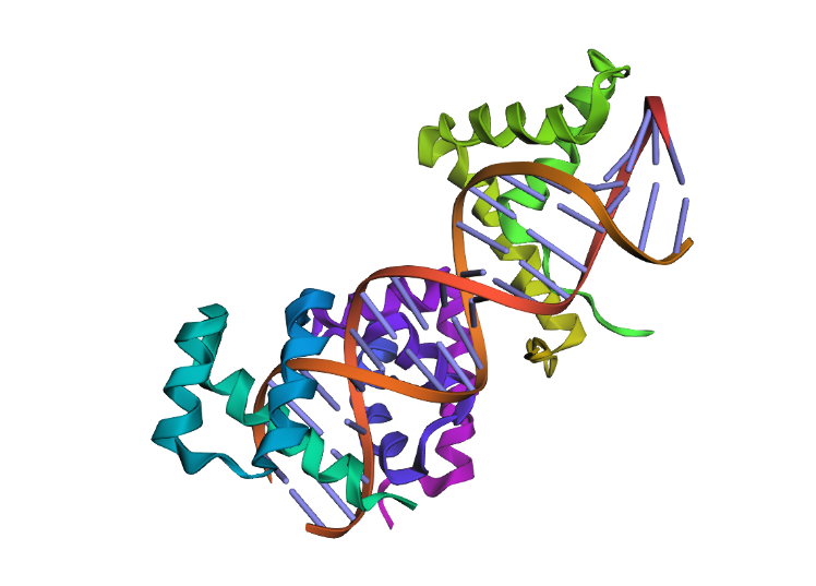
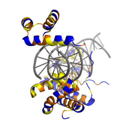
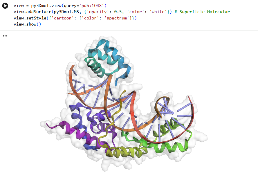
It was known since the 90’s that OCT4 and SOX2 can form a heterodimer that binds to a composite motif at thousands of sites in the genome, acting as pioneer trascription factors (the ones that maintains the accessibility of chromatin regions previously inaccessible).
Looking in the literature I found the degradation and protein stability values from OSK in mouse embryonic stem cells (ESC). These values were a reference, since the were obtained from studies in 2TS22C cell line and my cassete is intendent to be applied into old fibroblast
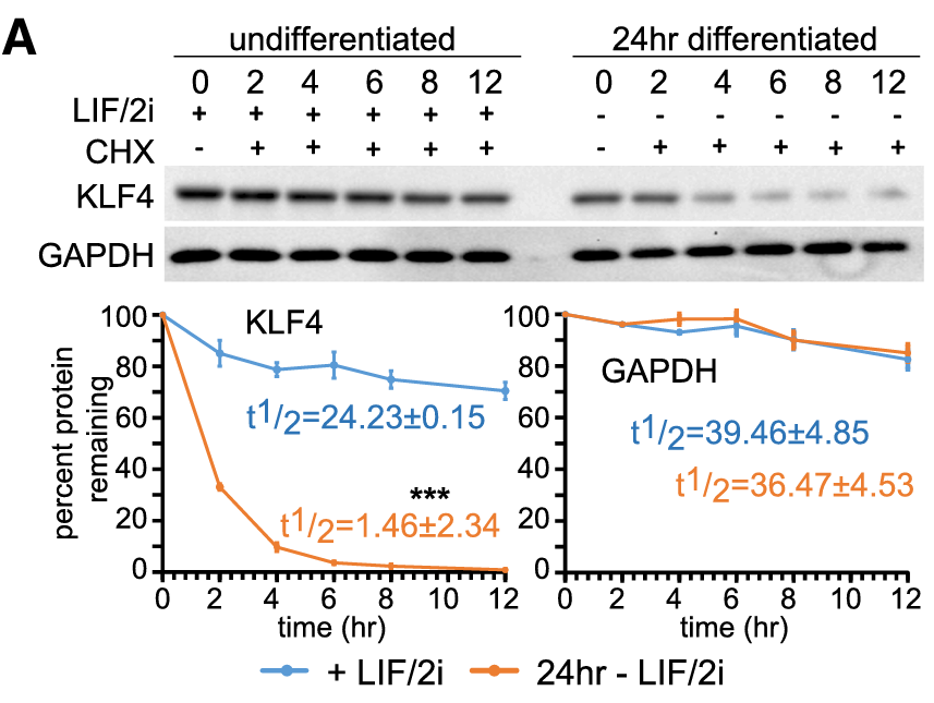
In the KLF4 protein case, Dhaliwal and peers in 2019 found that its stability was diminished in a 24h of differentiation ESC, but the presence of SOX2 and NANOG expression in differentiated cells restores KLF4 protein stability from t1/2 =2htot1/2=17 h in the case of Sox2 and from t1/2=1.5 h to t1/2=25 h in Nanog’s case.

Fig. 2.A from Dhaliwal et al. (2019) LIF referes to the Leukemia Inhibitory Factor serum in which the stem cells are cultivated to mantain cell plurypotency
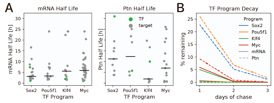
These proteins have different prevalence dependent on the cellular type being studied and the life stage of the cell. So, in order to get a better reference I used the half-life information indicated in the supplementary information of Roux et al. (2022), in which they considered the half-life of OSK factors in three days from being transfected into fibroblast
 Fig.S1 A and B from Roux et al. (2022) supplementary information
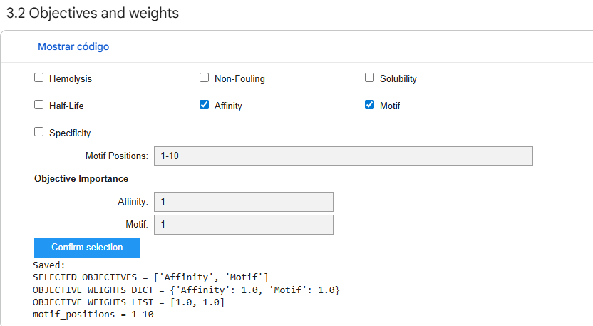
Now, with this search done, I proceded with a simple math model that will leverage iANNs loss function to optimize for the best promoters
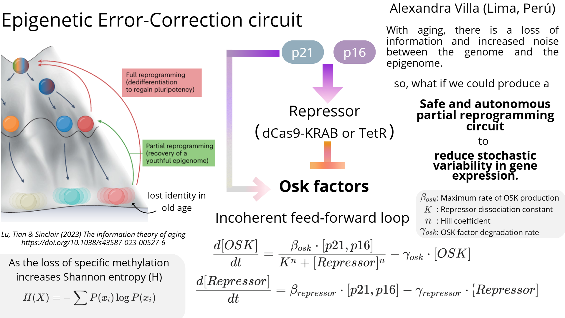
Mathematical Framework of the OSK Circuit
Formal Definition: The temporal evolution of the OSK concentration is modeled as a deterministic, continuous-time dynamical system. It is governed by a first-order ordinary differential equation (ODE) that balances non-linear thermodynamic synthesis with first-order kinetic decay.
The core mass-action kinetics of the system is defined by the following ODE:
$$ \frac{d[OSK]}{dt} = \alpha_{0} + \alpha - \gamma[OSK] $$
Where each term represents a distinct biophysical process:
Computational Integration: Rather than relying on arbitrary parameters, this ODE serves as the explicit physics constraint within our Physics-Informed Neural Network (PINN). By embedding this differential topology into the model's loss function, we ensure that in silico sequence designs strictly adhere to real-world kinetic boundaries.
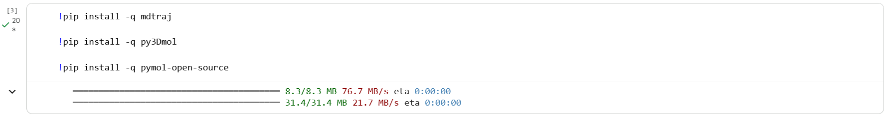
Now, since I’m still on diapers when it comes to programming, with help of Gemini.AI I code a synthetic transcriptome with the gathered information, almost all based on Roux et al. (2022), like the OSK ARNm virtually indicating 0 on the 10th and 15th days, just like the remaining < 0.05% remaining they got.
```
import numpy as np
import scanpy as sc
import anndata as ad
import pandas as pd
print("Generando transcriptoma sintético de MEFs con datos empíricos...")

# 1. Definimos los días de recolección (Pulse: 0 a 7, Chase: 7 a 15)
dias = [0, 3, 7, 10, 15]
celulas_por_dia = 200

# =========================================================================
# PARÁMETROS EMPÍRICOS EXTRAÍDOS DE LA LITERATURA
# =========================================================================
# Vidas medias de ARNm [horas] (Roux et al. Supplementary Information - Fig S1)
t_half_Pou5f1 = 3.2
t_half_Sox2 = 3.1
t_half_Klf4 = 5.5  # Nota: Dhaliwal et al. reporta >24h en ES, pero usamos el de transito de Roux

# Calculamos la constante de decaimiento kd en [días^-1] (kd = ln(2) / t_half_dias)
# Esto dictará la caída exponencial durante la fase de "Chase"
kd_Pou5f1 = np.log(2) / (t_half_Pou5f1 / 24)  # ~5.2 días^-1
kd_Sox2   = np.log(2) / (t_half_Sox2 / 24)    # ~5.3 días^-1
kd_Klf4   = np.log(2) / (t_half_Klf4 / 24)    # ~3.0 días^-1

X_list = []
obs_list = []

for t in dias:
    # -----------------------------------------------------------------
    # A. DINÁMICA DE LA IDENTIDAD SOMÁTICA (Col1a1, Thy1)
    # -----------------------------------------------------------------
    # [Paper: Roux et al. "Partial reprogramming transiently suppresses somatic identity"]
    # La expresión baja durante la inducción y se recupera tras el chase.
    if t <= 7:
        # Supresión transitoria durante el pulso
        media_somatica = 10 - t
        varianza = 0.5 + (t * 0.5) # Critical Slowing Down hacia la bifurcación
    else:
        # Re-establecimiento de la identidad tras retirar los factores
        delta_t_chase = t - 7
        media_somatica = 3 + (delta_t_chase * 0.8) # Recuperación lineal/exponencial
        varianza = 1.5

    genes_somaticos = np.random.normal(loc=media_somatica, scale=varianza, size=(celulas_por_dia, 2))
    genes_somaticos = np.clip(genes_somaticos, a_min=0, a_max=None) # No hay scRNA-seq negativo

    # -----------------------------------------------------------------
    # B. DINÁMICA DE LOS FACTORES DE REPROGRAMACIÓN (Pou5f1, Sox2, Klf4)
    # -----------------------------------------------------------------
    # [Paper: Roux et al. Suppl. Info - EDO decay model: p(t) = p(0)e^(-kt)]
    if t <= 7:
        # Fase PULSE: Acumulación hasta estado estacionario (steady-state)
        # Simulamos que alcanzan un nivel máximo (ej. log1p CPM = 8)
        media_Pou5f1 = t * 1.1
        media_Sox2   = t * 1.1
        media_Klf4   = t * 1.1
    else:
        # Fase CHASE: Decaimiento cinético estricto según kd empírico
        delta_t_chase = t - 7
        # Nivel máximo alcanzado en el día 7
        max_expr = 7 * 1.1

        # p(t) = p(0) * exp(-kd * t)
        media_Pou5f1 = max_expr * np.exp(-kd_Pou5f1 * delta_t_chase)
        media_Sox2   = max_expr * np.exp(-kd_Sox2 * delta_t_chase)
        media_Klf4   = max_expr * np.exp(-kd_Klf4 * delta_t_chase)

        # [Paper: Roux et al. - "By day 3 of chase, < 0.05% of mRNA remains"]
        # Las medias a partir del día 10 tenderán asintóticamente a 0 rápidamente.

    # Añadimos ruido técnico típico de scRNA-seq (ruido Poisson/Normal)
    gen_Pou5f1 = np.random.normal(loc=media_Pou5f1, scale=0.5, size=(celulas_por_dia, 1))
    gen_Sox2   = np.random.normal(loc=media_Sox2,   scale=0.5, size=(celulas_por_dia, 1))
    gen_Klf4   = np.random.normal(loc=media_Klf4,   scale=0.5, size=(celulas_por_dia, 1))

    genes_reprog = np.hstack([gen_Pou5f1, gen_Sox2, gen_Klf4])
    genes_reprog = np.clip(genes_reprog, a_min=0, a_max=None)

    # -----------------------------------------------------------------
    # C. ENSAMBLAJE DE LA MATRIZ DEL TIEMPO t
    # -----------------------------------------------------------------
    X_t = np.hstack([genes_somaticos, genes_reprog])
    X_list.append(X_t)

    # Metadatos
    obs_t = pd.DataFrame({
        'time_days': [t] * celulas_por_dia,
        'phase': ['Pulse' if t <= 7 else 'Chase'] * celulas_por_dia
    })
    obs_list.append(obs_t)

# 3. Ensamblamos el objeto AnnData (.h5ad)
X_total = np.vstack(X_list)
obs_total = pd.concat(obs_list, ignore_index=True)
var_total = pd.DataFrame(index=["Col1a1", "Thy1", "Pou5f1", "Sox2", "Klf4"])

adata_simulado = ad.AnnData(X=X_total, obs=obs_total, var=var_total)

# 4. Guardamos el archivo
ruta_archivo = "mef_simulado_parametros_empiricos.h5ad"
adata_simulado.write_h5ad(ruta_archivo)

print(f"¡Éxito! Archivo {ruta_archivo} creado.")
```
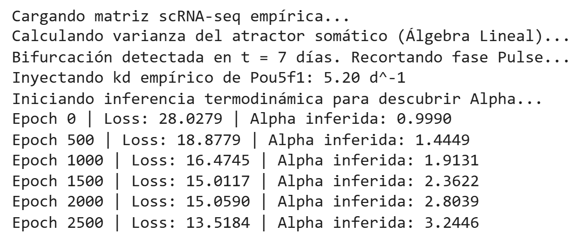
Then, the next step was coding the iANNs training to find the most suitable rate of transcription to match the incoherent feed-forward loop I was planning to add in the plasmid. So, again with Gemini’s help, the code was:
```
import torch
import torch.nn as nn
import scanpy as sc
import numpy as np
  # =====================================================================
  # 1. MÓDULO DE FÍSICA ESTADÍSTICA (Scanpy para Critical Slowing Down)
  # =====================================================================
  def extract_critical_dynamics(h5ad_path, somatic_genes, osk_gene_name):
      """
      Lee datos scRNA-seq, calcula la varianza somática para detectar el
      punto de bifurcación y extrae tensores para PyTorch.
      """
      print("Cargando matriz scRNA-seq empírica...")
      adata = sc.read_h5ad(h5ad_path)

      time_points = sorted(adata.obs['time_days'].unique())
      variances = []
      osk_means = []

      print("Calculando varianza del atractor somático (Álgebra Lineal)...")
      for t in time_points:
          cells_t = adata[adata.obs['time_days'] == t]

          X_somatic = cells_t[:, somatic_genes].X
          if hasattr(X_somatic, "toarray"):
              X_somatic = X_somatic.toarray()

          # Varianza como trazador de inestabilidad termodinámica
          var_t = np.var(X_somatic)
          variances.append(var_t)

          osk_expr = cells_t[:, osk_gene_name].X
          if hasattr(osk_expr, "toarray"):
              osk_expr = osk_expr.toarray()
          osk_means.append(np.mean(osk_expr))

      t_crit_idx = np.argmax(variances)
      t_crit = time_points[t_crit_idx]
      print(f"Bifurcación detectada en t = {t_crit} días. Recortando fase Pulse...")

      # Extraemos solo la fase "Pulse" (donde alpha está activo buscando el steady-state)
      t_empirical = np.array(time_points[:t_crit_idx + 1], dtype=np.float32).reshape(-1, 1)
      osk_empirical = np.array(osk_means[:t_crit_idx + 1], dtype=np.float32).reshape(-1, 1)

      t_tensor = torch.tensor(t_empirical, requires_grad=True)
      osk_tensor = torch.tensor(osk_empirical)

      return t_tensor, osk_tensor, t_crit


  import torch
  import torch.nn as nn

  # =====================================================================
  # 2. ARQUITECTURA PINN IFFL (Incoherent Feed-Forward Loop)
  # =====================================================================
  class iANN_OSK_IFFL(nn.Module):
      def __init__(self, kd_empirico):
          super(iANN_OSK_IFFL, self).__init__()
          self.net = nn.Sequential(
              nn.Linear(1, 32),
              nn.Tanh(),
              nn.Linear(32, 32),
              nn.Tanh(),
              nn.Linear(32, 1)
          )

          # PARÁMETROS QUE LA RED DEBE DESCUBRIR
          self.alpha = nn.Parameter(torch.tensor([5.0])) # Tasa transcripcional máxima

          # PARÁMETROS FÍSICOS FIJOS (Conocimiento a priori del IFFL)
          self.kd = kd_empirico

          # Parámetros del Represor (Puedes volverlos nn.Parameter si quieres que la red los infiera)
          self.tau = 1.5 # Retraso temporal (ej. 1.5 días / 36 horas para que empiece a frenar)
          self.n_hill = 3.0 # Coeficiente de Hill (cooperatividad del represor)
          self.k_represor = 2.0 # Qué tan rápido se acumula el represor tras el retraso

      def forward(self, t):
          return self.net(t)

  def compute_physics_loss_iffl(model, t_collocation):
      t_collocation.requires_grad = True
      OSK_pred = model(t_collocation)

      # 1. Diferenciación Automática para hallar d[OSK]/dt
      dOSK_dt = torch.autograd.grad(
          outputs=OSK_pred,
          inputs=t_collocation,
          grad_outputs=torch.ones_like(OSK_pred),
          create_graph=True
      )[0]

      # 2. Ecuación del Represor (Variable Latente)
      # Modelamos el represor [R] saturando el promotor después del tiempo tau
      # Usamos una sigmoide (función logística) para simular la acumulación del represor en el tiempo
      R_t = torch.sigmoid(model.k_represor * (t_collocation - model.tau))

      # 3. Función de inhibición de Hill: 1 / (1 + R^n)
      # Si R_t es 0 (antes de tau), el freno es 1 (faucet abierto).
      # Si R_t es 1 (después de tau), el freno tiende a 0 (faucet cerrado).
      freno_transcripcional = 1.0 / (1.0 + R_t ** model.n_hill)

      # 4. Nuevo Residual de la EDO con el IFFL incorporado
      produccion_real = model.alpha * freno_transcripcional
      residual = dOSK_dt - produccion_real + (model.kd * OSK_pred)

      return torch.mean(residual ** 2)

  # =====================================================================
  # 3. BUCLE DE ENTRENAMIENTO INTEGRADO
  # =====================================================================
  def train_pinn(model, t_data, OSK_data, epochs=3000):
      optimizer = torch.optim.Adam(model.parameters(), lr=1e-3)
      mse_loss_fn = nn.MSELoss()

      print("Iniciando inferencia termodinámica para descubrir Alpha...")
      for epoch in range(epochs):
          optimizer.zero_grad()

          # A. Pérdida Empírica (ScRNA-seq data)
          OSK_pred_data = model(t_data)
          loss_data = mse_loss_fn(OSK_pred_data, OSK_data)

          # B. Pérdida Física Continua
          t_collocation = torch.rand(100, 1) * t_data.max().item()
          loss_ode = compute_physics_loss(model, t_collocation)

          # C. Gradiente Global
          loss_total = loss_data + (0.5 * loss_ode)

          loss_total.backward()
          optimizer.step()

          if epoch % 500 == 0:
              print(f"Epoch {epoch} | Loss: {loss_total.item():.4f} | Alpha inferida: {model.alpha.item():.4f}")

  # =====================================================================
  # 4. EJECUCIÓN DEL PIPELINE
  # =====================================================================
  if __name__ == "__main__":
      # 1. Usamos el nuevo archivo con la métrica real
      ruta_geo = "mef_simulado_parametros_empiricos.h5ad"

      # 2. Genes reales del nuevo script (quitamos Fap que ya no está)
      genes_fibroblasto = ["Col1a1", "Thy1"]
      gen_diana = "Pou5f1"

      t_emp, osk_emp, t_c = extract_critical_dynamics(ruta_geo, genes_fibroblasto, gen_diana)

      # 3. Constantes empíricas (Paper: Roux et al. Suppl. Fig S1)
      # Pou5f1 mRNA half-life ~ 3.2 horas -> ~0.1333 días
      # kd = ln(2) / t_half = 5.2 días^-1
      kd_Pou5f1_empirico = np.log(2) / (3.2 / 24.0)
      print(f"Inyectando kd empírico de Pou5f1: {kd_Pou5f1_empirico:.2f} d^-1")

      # 4. Entrenamos
      modelo_osk = iANN_OSK(kd_empirico=kd_Pou5f1_empirico)
      train_pinn(modelo_osk, t_emp, osk_emp)
```
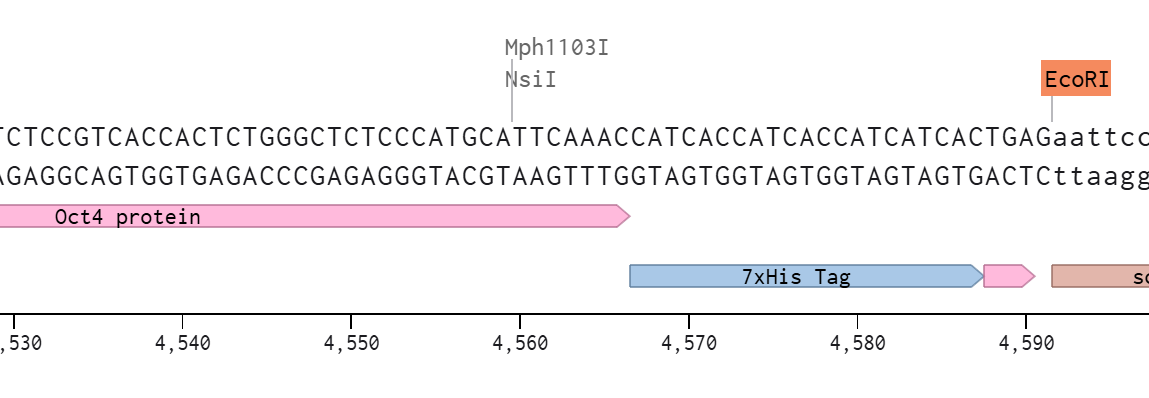
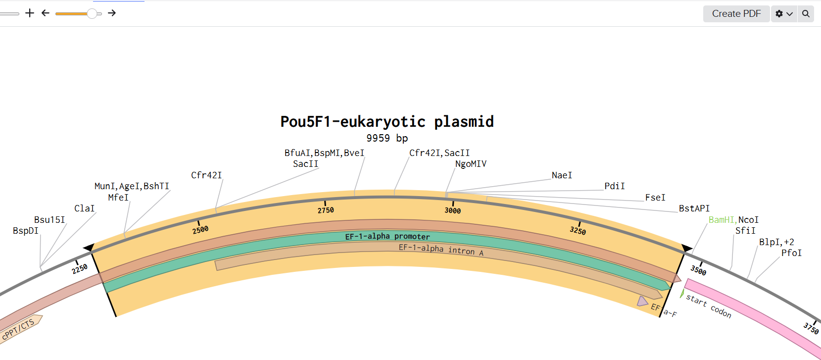
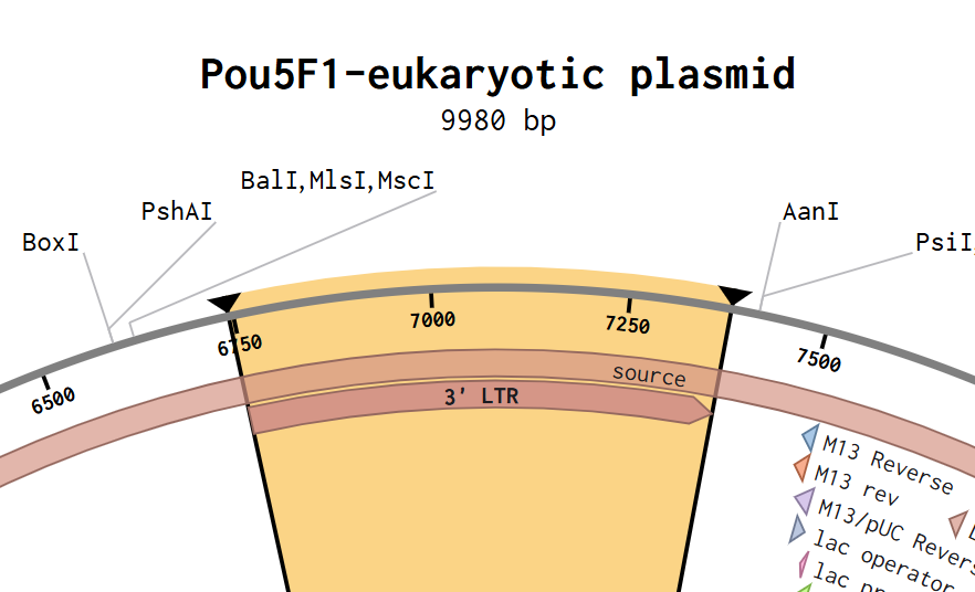
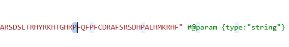
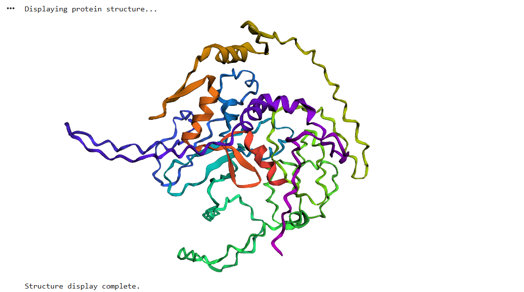
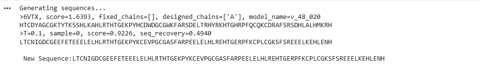
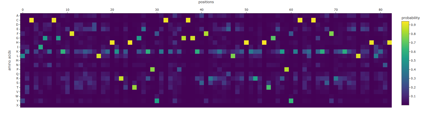
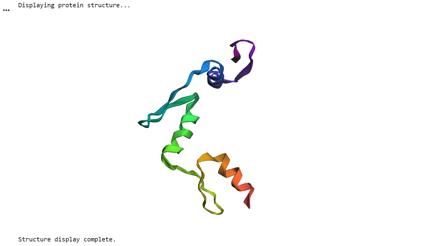
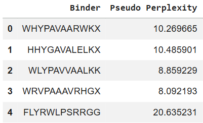
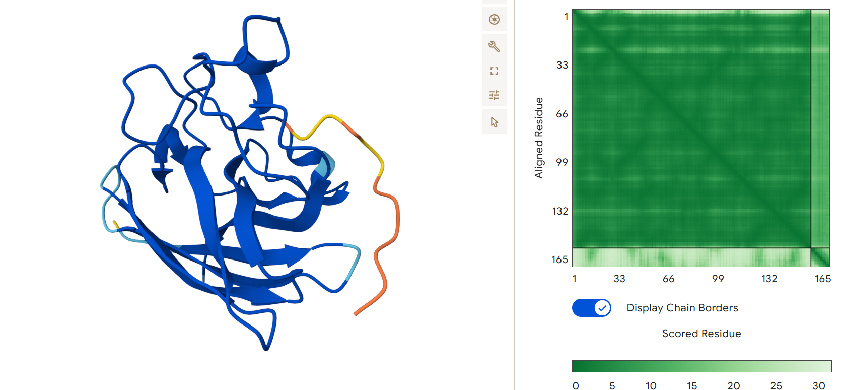
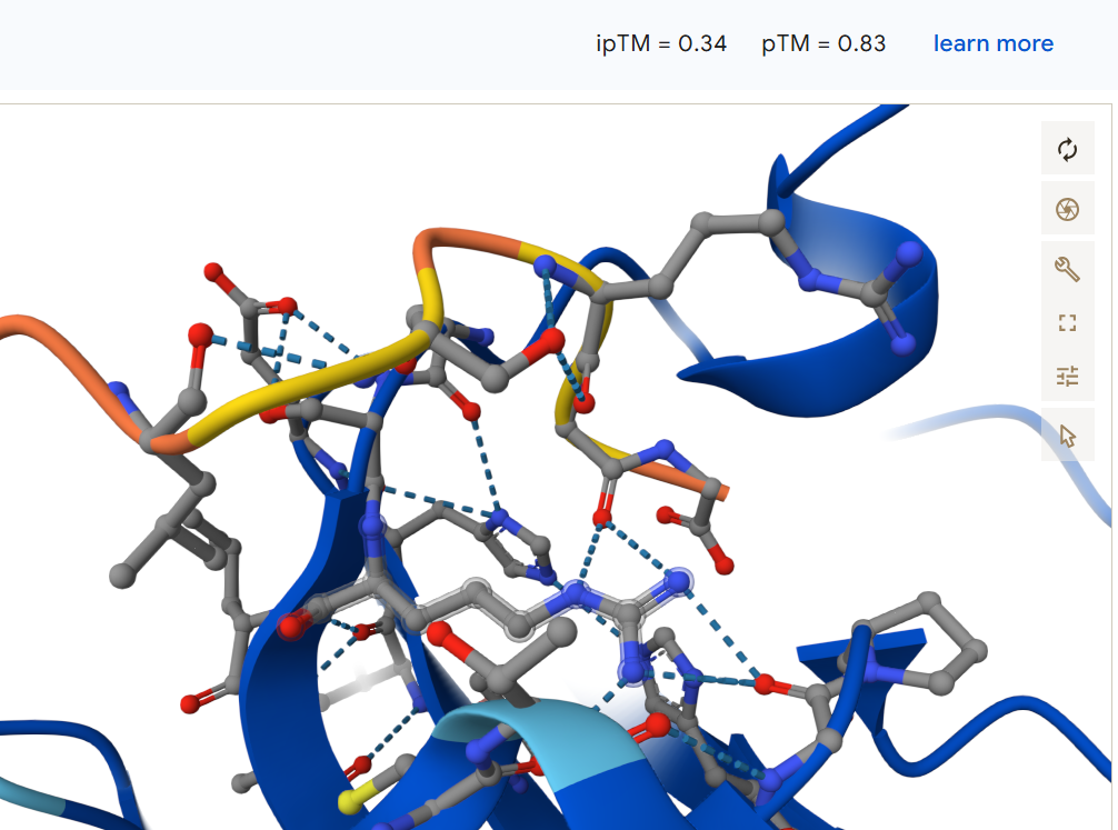
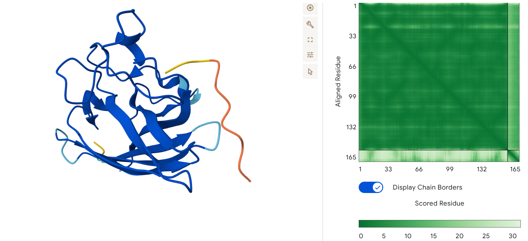
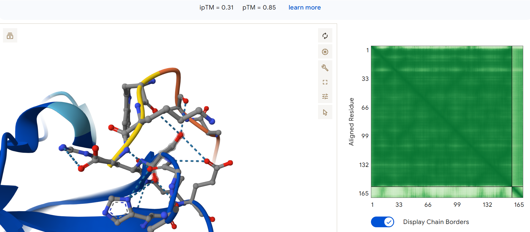
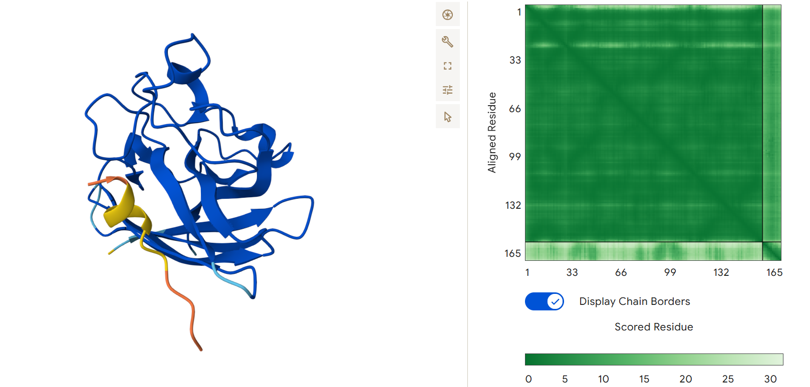
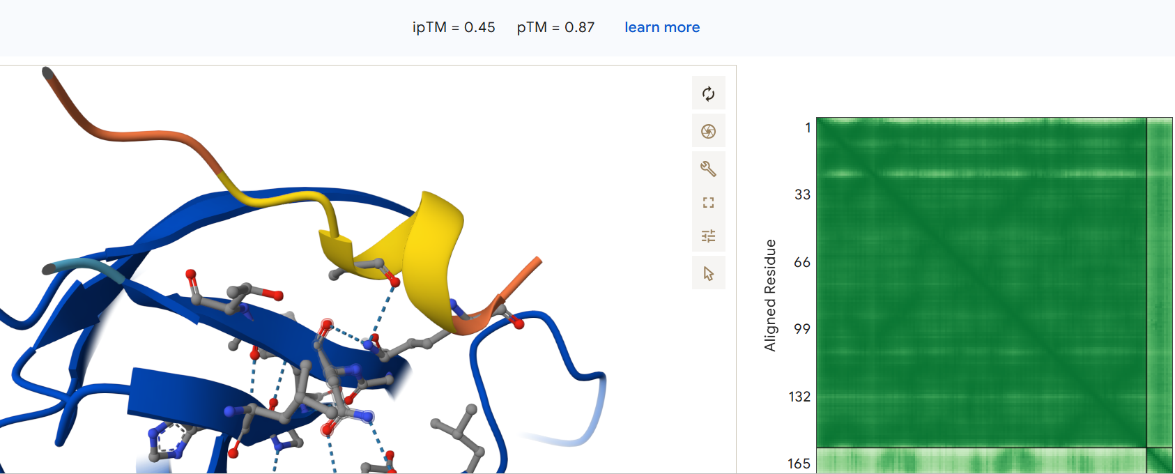
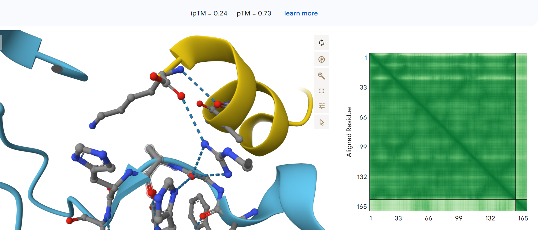
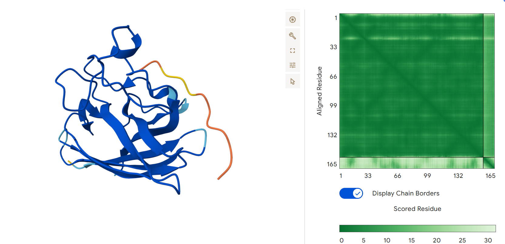
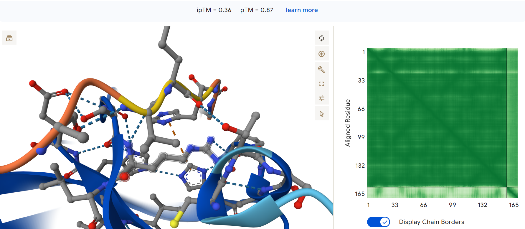
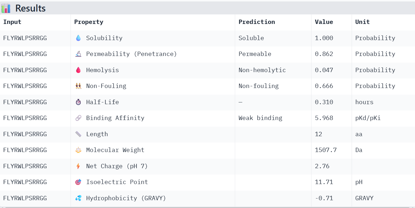
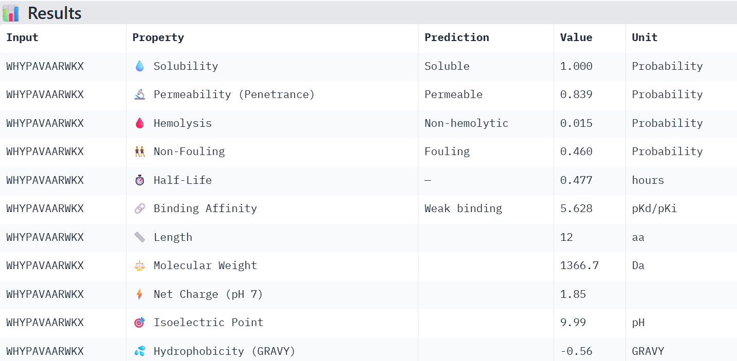
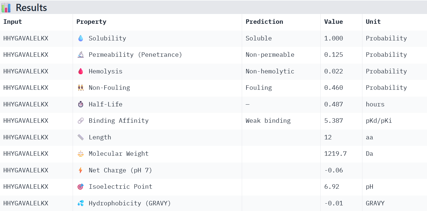
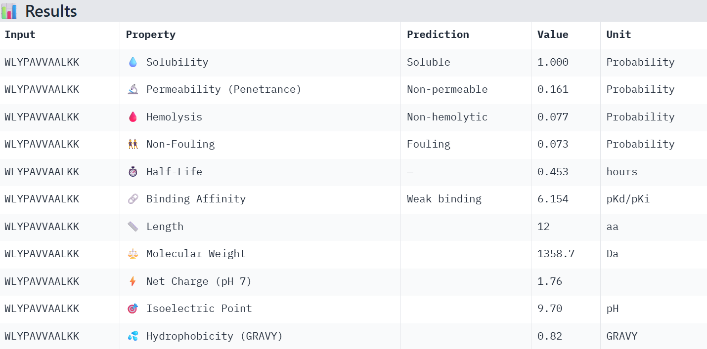
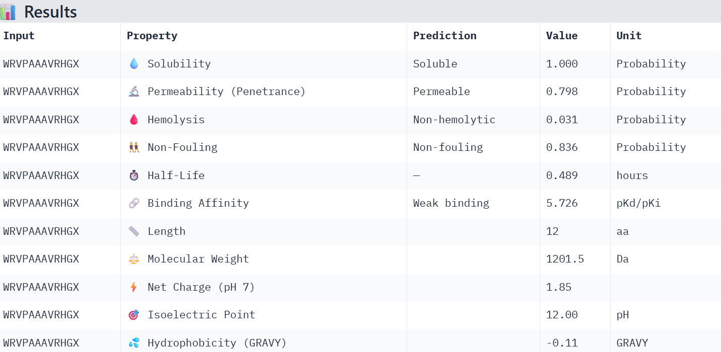
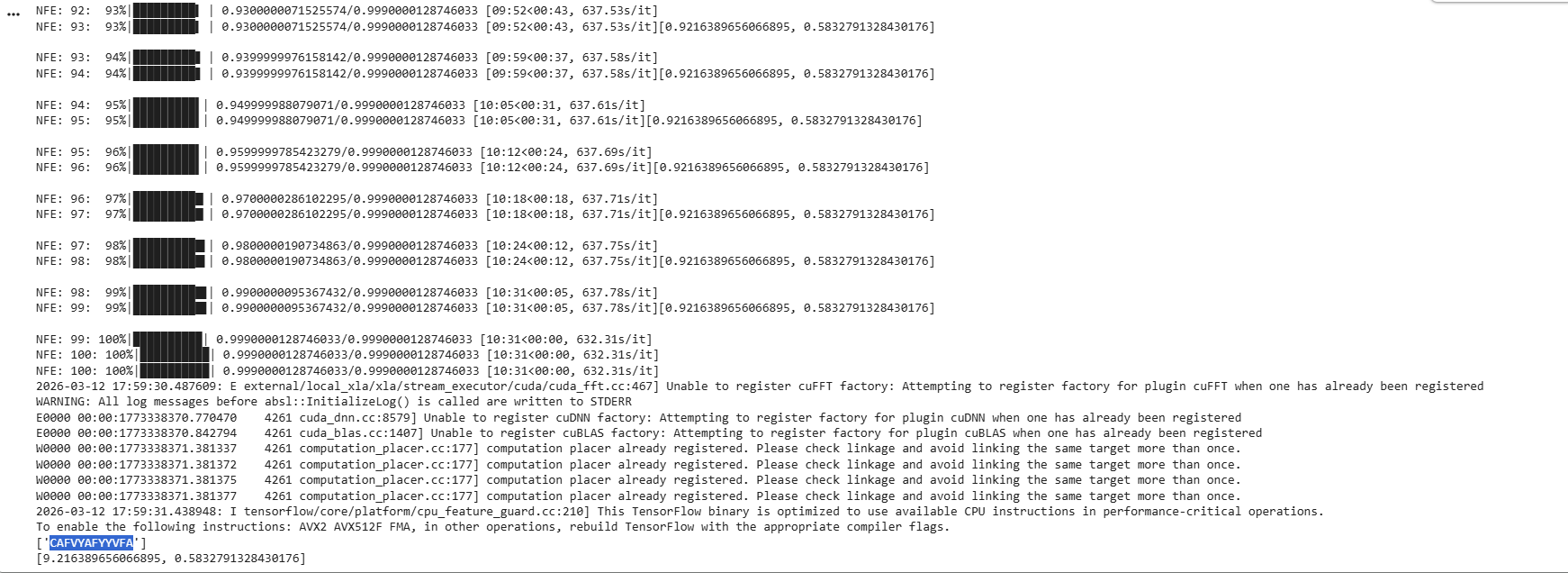
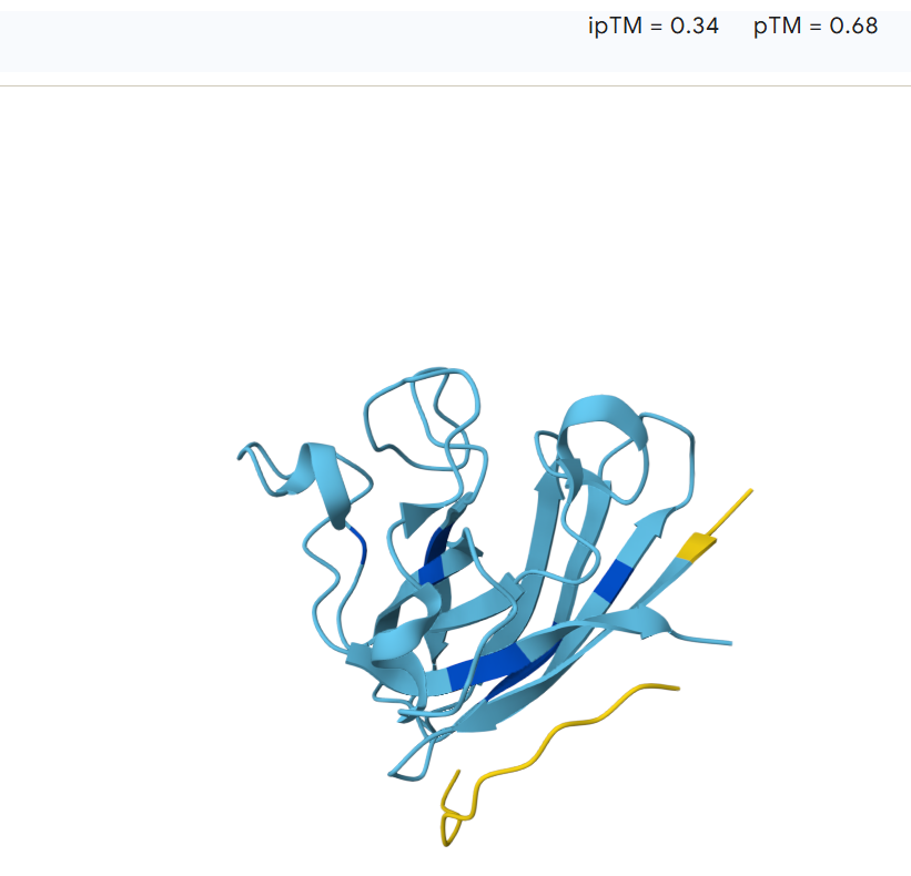
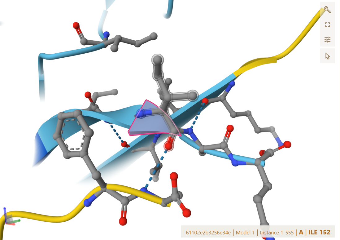
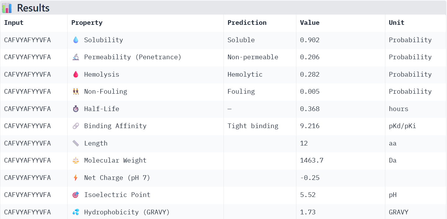
Finally obtaining