Week 1 HW: Principles and Practices

Living lab TerraPods, Lebanon

The halfpipe of Doom- How to grow good?

For the first weeks lecture we had an introduction to the fundamental principles of synthetic biology and the HTGAA program. The focus of the lecture was on the governance and ethics of synthetic biology. David S. Kong discussed the balance between decentralized and centralized synBio development and the importance of thrust (something we are lacking these days). As a global community we have largely agreed to certain rules (e.g. bioweapon treaty 1975) however emerging synBio technologies also allow a much broader audience to participate in the development (e.g. community labs/ biohackers) that might not necessary always align with large governmental policies. He draws the parallel to how the early governance of the internet have allowed for a decentralized scaling that have contributed to an increased “computer literacy”. This might allow us to make better (although not perfect) personal decisions for how to use this new technology. Coming from a background of community focused biolab practice this was an interesting topic and made me think of the importance for a global bio-literacy. It also got me to think about the importance to apply these principals in a simple enough way that it doesn’t stifle participation.

Questions that I tried to include in my homework:

1. Describe a biological engineering application

Programmable colors for bacterial cellulose production

The textile dyeing industry is a major source of chemical pollution and water use. Coloration of bacterial cellulose (BC) can also be technically challenging because pigments often diffuse slowly into the material’s dense nanofibrillar network, making post-growth dyeing difficult and time consuming. This project proposes a bioengineering approach to generate color in situ during BC growth, eliminating conventional dyeing steps.

Dyed BC I developed at TerraPods Lebanon

Prior work demonstrates the feasibility of embedding pigmentation into BC production. Walker et al.(2025) ¹ engineered the cellulose-producing bacterium Komagataeibacter rhaeticus to generate melanin during BC growth, producing pigmented material. Zhou et al. (2025) ² demonstrated a “one-pot” co-culture strategy coupling BC production by Komagataeibacter xylinus with pigments synthesised in engineered E. coli, enabling a broader palette by combining violacein derivatives (green/blue/navy/purple) and carotenoids (red/orange/yellow).

Zhou et al. (2025)

Building on these studies, the core concept here is light-patterned control of pigment production during BC formation. A cellulose-forming culture generates the sheet while a pigment-producing bacteria is engineered to be light-responsive, so that pigmentation occurs in illuminated regions. Patterned illumination via projection enables spatial control of coloration. Furthermore this technique would also enable varying projected patterns across growth phases that could yield multi-layer visual effects, (e.g. moiré-like effects).

Walker et al.(2025)

Drawing from my previous experiences on working in various community biolab the project is framed as a distributed biofabrication platform for community labs, which creates governance questions around biosafety practice in a decentralized settings, concider the relative complex technique I was for this excersice imagining a centralized organization providing the framework and digital infrastructure for the community labs to safetly experiment with the protocol. Although consumer product are less ethically complicated then for example medicine or bioweapon their came up important questions concerning consumer/skin-contact safety, environmental release and waste handling, and norms for responsible dissemination of methods and bacteria strains.

2. governance/policy goals

                CENTRAL PLATFORM / ORG
     (protocol repo + training + registry + reporting)
            |           |               |
     SOP minimums   pigment safety   open hardware stack
     (Option 1)      (Option 2)          (Option 3)
            |           |               |
            +-----------+---------------+
                        |
        -----------------------------------------
        |                  |                   |
   Community Lab A     Community Lab B     Community Lab C...
 (local biosafety)   (local biosafety)   (local biosafety)
   - containment        - containment       - containment
   - waste handling     - waste handling    - waste handling
   - incident reports   - incident reports  - incident reports
   - minimal tests + labeling (skin-contact, leaching, etc.)
                        |
  Local authorities / partners / funders
  (disposal rules, validation support, incentives)

• Actors: Community labs and networks, open-hardware designers, academic partners, funders, and (optionally) insurers.

A. Biosecurity

• A1: Reduce risk of malicious repurposing of organisms, materials, or protocols.
• A2: Improve traceability and incident reporting to support response.

B. Lab safety

• B1: Standardize safe practices (training, containment, waste handling) across labs.
• B2: Establish clear response procedures for spills, exposures, and contamination.

C. Environmental protection

• C1: Prevent release of organisms or harmful pigments/byproducts.
• C2: Enable remediation and corrective action after incidents.

D. User/consumer protection and social trust

• D1: Ensure skin-contact safety (low leaching, low irritation risk, stability).
• D2: Maintain low barrier access; avoid governance that excludes low-resource labs.
• D3: Require transparency and avoid misleading sustainability claims.

E. Feasibility and innovation

• E1: Keep requirements simple for community labs.
• E2: Avoid unnecessary friction to legitimate research and education.

3. Governance actions (three options)

➡️ Option 1 — Network baseline: certification + SOP minimums

Purpose: Reduce variability in biosafety practice across distributed labs.

Design: A lightweight participation standard for labs using the platform including training checklist; Standard operating procedure (SOP) templates for handling, contamination response, waste logs and periodic documentation checks.

Assumptions: Labs will opt in if benefits are tangible and the extra admistrive work is not to burdensome.

Risks: Uneven enforcement; exclusion of under-resourced labs if standards become to complex.

➡️ Option 2 — Pigment/material safety standard: whitelist + minimal testing + labeling

Purpose: Address the most important downstream risk for the product: skin-contact, pigment safety and environmental implications.

Design: Shared “allowable pigment classes” (whitelist) plus minimum evidence requirements for testing (basic leach, washfastness, disposal guidance, documentation of lab status). Standard labeling for intended use and safety-relevant claims.

Assumptions: Low-cost testing tools or institutional partners are available; whitelist stays current and not to restrictive.

Risks: The process to complex and hindering community engagement, or weak tests gives unreliable results, slowed innovation if the whitelist narrows too far.

➡️ Option 3 — Open-source hardware standards for safe, distributed BC biofabrication

Purpose: Reduce reliance on expensive proprietary equipment while lowering barriers to participation without lowering safety. The goal is to make safe practice easier by default through standardized, well-documented hardware and workflows suitable for community labs.

Design: an open-source “reference stack” that includes:

• Validated hardware designs for core needs (e.g., enclosed growth modules with spill containment, filtered airflow concepts, light/projection enclosures to reduce eye/UV exposure, basic sensing/logging for temperature/pH proxies where appropriate).
• A documentation package: build BOMs with substitutions, maintenance/calibration checklists, cleaning/decon compatibility notes, and safety labels.
• Inter-lab benchmarking: common test artifacts and reporting templates so labs can compare performance and identify failure modes early.

Assumptions:

• Standardizing equipment and documentation will reduce accidents and variability more effectively than rules alone.
• Community labs have enough fabrication capacity (or partner access) to build/maintain hardware.
• A shared reference design can remain adaptable across different local constraints.

Risk:

• Hardware reliability varies; incomplete documentation leads to unsafe modifications; lack of maintenance causes drift in performance.
• Lowered barriers increase scale of adoption faster than training capacity; designs are copied without safety context; fragmentation into many forks undermines standardization.

4. Score

5. Prioritization and recommendation

I would prioritize Option 1 + Option 2 as the baseline governance package, with Option 3 as a longer-term technical pathway. Option 1 provides uniform safety culture and response capacity across labs; Option 2 directly governs consumer-contact risks and environmental externalities specific to pigment-enabled textiles. Option 3 is desirable for uniformed implementation of option 1 and 2 in a community lab setting.

Primary audiences: community lab networks and lab leads (implementation), funders/partners, and local safety/environment authorities (alignment on waste and disposal practices).

ChatGBT 5.2 was used for brainstorming bioengineering ideas for BC production in a community based setting

Aswell as searching for academic literature

and correct spelling error and double checking if I understood the research correctly

and to make the code for the governance chart:

It was also used for debugging some of the problems that I had with the website build, I am not including those prompts here…

Homework Questions from Professor Jacobson

Homework Questions from Dr. LeProust:

Homework Question from George Church:

Week 2 HW: dna read write and edit

Part 1: Benchling & In-silico Gel Art

My original idea was to make a circle, but after some trial and error I realized it would be a bit too complicated—so I settled on an arch (bridge).

1a) I imported the sequence for lambda DNA.

1b) In Benchling, I ran all 7 restriction enzymes we had available to see which ones gave:

• a busy lane (many bands) → use as the “background” in most lanes
• a cleaner lane (fewer bands) → use to “carve out” the interior of the arch

Note:

• Lane = the vertical track DNA runs down from a single well
• Bands = the horizontal lines within a lane (different fragment sizes)

Based on the results above, I rearranged the enzymes to create the pattern:

Although it’s not the most beautiful arch, this was a great exercise for understanding the basics of in-silico digests and gel band patterns.

This tool is also great for quickly iterating on gel-art layouts: https://rcdonovan.com/gel-art

3.1. Choose your protein

In recitation, we discussed picking a protein for the homework that you personally find interesting. I chose CBM3.

Why CBM3?
CBM3 is interesting because it works like a modular “cellulose anchor”: you can fuse it to other proteins so they reliably stick to cellulose (including bacterial cellulose). Beyond simple labeling, CBM fusions are used as fluorescent probes to visualize cellulose organization and dynamics, as affinity tags for low-cost purification on cellulose, and as anchoring domains to immobilize enzymes on cellulose scaffolds—turning cellulose into a reusable biocatalyst support or functional capture material.

Simply put: it’s short, often expresses well, and it sticks to cellulose.
Reference: CBM3 (example paper)

In UniProt, I searched for “carbohydrate-binding module CBM cellulose-binding protein” and got many hits. A good way to narrow the options is to pick something that is:

1. Reviewed (Swiss-Prot) (more reliable annotation)
2. Short / manageable (ideally ~80–250 aa)
3. Clearly annotated as a CBM domain (cellulose-binding)

The UniProt entry I used was Q06851. The full protein is long, but UniProt makes it possible to extract only the domain/region relevant to the application:

1. Open the UniProt entry
2. Scroll to Family & Domains
3. Find the feature you are interested in (domain boundaries)

I chose the CBM3 (carbohydrate-binding module family 3) from the cellulosome scaffoldin CipA, because CBM3 specifically binds cellulose and is relevant for bacterial cellulose materials.

3.2. Reverse translate: Protein (amino acid) → DNA (nucleotide)

To extract only the CBM3 region, I downloaded the sequence and used the Gao Lab WebLab tool:
WebLab – range_extract_protein

I entered the range 365–523, which returned:

>CBM3_CipA_Q06851_res365-523
GAYAITKDGVFAKIRATVKSSAPGYITFDEVGGFADNDLVEQKVSFIDGGVNVGNATPTKGATPTNTATPTKSATATPTRPSVPTNTPTNTPANTPVSGNLKVEFYNSNPSDTTNSINPQFKVTNTGSSAIDLSKLTLRYYYTVDGQKDQTFWCDHAAI

Next, I pasted the CBM3 amino-acid sequence into the Sequence Manipulation Suite reverse-translation tool: bioinformatic – Reverse Translate

Finally, I double-checked the result in Benchling by pasting the reverse-translated DNA into a new sequence and using Benchling’s Translate feature to confirm it produced the same amino-acid sequence.

3.3. Codon optimization

I decided to codon-optimize for E. coli because it’s a common protein-expression host with well-established tools. Codon optimization matters because organisms have different codon bias / tRNA abundances, and matching preferred codons often improves translation efficiency, protein yield, and reduces stalling during expression. To do this, I used Twist’s codon-optimization workflow and selected Host: Escherichia coli. The optimization completed successfully (“Optimization was successful”) and the sequence scored Standard, indicating it is considered synthesize-able under Twist’s constraints. I then selected Use the optimized sequence and (as a sanity check) confirmed that the translated amino-acid sequence remained unchanged—only synonymous codons were swapped.

“I optimized for E. coli because it’s a common protein-expression host with well-established tools; the purified CBM can then be applied to bacterial cellulose to bind it.”

3.4. You have a sequence! Now what?

Now that I have a DNA sequence encoding CBM3, the next step is to express the protein. In a typical cell-dependent (in vivo) workflow, the codon-optimized CBM3 coding sequence is cloned into an E. coli expression plasmid under a promoter (e.g., T7/lac).

-An expression plasmid is designed to make lots of protein.

-A promoter is a DNA “on-switch” that tells the cell when to start making RNA from your gene.

-T7/lac is a common strong promoter system used to tightly control expression.

After transforming the plasmid into an expression strain, the cells are grown and expression is induced (often with IPTG).

IPTG releases repression in the lac system so the promoter becomes active, and the cells start producing CBM3.

Inside the cell, the DNA is transcribed by RNA polymerase into mRNA, and the mRNA is then translated by ribosomes into the CBM3 protein as tRNAs deliver amino acids according to the codons. The protein can then be purified (for example via an affinity tag such as His-tag) and used to bind/functionalize bacterial cellulose.

-His-tag lets you purify CBM3 using a matching resin (Ni-NTA), washing away everything else.

Alternatively, CBM3 could be produced using a cell-free expression system (TX-TL), where the DNA template (plasmid or linear) is added directly to a lysate containing RNA polymerase, ribosomes, and all required cofactors.

required cofactors: -RNA polymerase

-ribosomes

-tRNAs, amino acids

-energy + cofactors

In this setup the same steps—transcription to mRNA and translation to protein—happen in a test tube rather than inside living cells, which can be faster and easier for prototyping, though often at smaller scale.

Why do cell-free?

• Often faster for prototyping (no transformations, no growing cells).
• Convenient when testing multiple designs quickly.
• Downsides: usually more expensive per mg and often smaller scale/yield than growing E. coli.

Ethical and regulatory difference: Cell-free systems are generally considered safer because they are non-living reactions that cannot usually replicate or spread in the environment. They stop once substrates, energy, or cofactors are depleted. In contrast, in-cell genetic engineering uses living organisms, which can continue growing and may pose risks if accidentally released, such as persistence in the environment or transfer of engineered DNA to other organisms.

Part 4 — Build an E. coli expression cassette (Benchling → Twist-ready)

For this step I designed a complete E. coli expression DNA insert in Benchling by assembling the required genetic parts in the correct order:

1. Promoter (BBa_J23106)
2. RBS (BBa_B0034 + spacer)
3. Start codon (ATG)
4. Coding sequence: replaced the template CDS with my codon-optimized gene (from Part 3)
5. C-terminal His-tag (7×His)
6. Stop codon (TAA)
7. Terminator (BBa_B0015)

After pasting each piece, I annotated every region (promoter, RBS, start, CDS, His-tag, stop, terminator) directly on the Benchling sequence.

benchling

I also used Benchling’s Analyze/Translate to confirm the ATG (Open Reading Frame) is in frame from the ATG (Start codon) and that the sequence ends with the His-tag followed by a stop codon.

Benchling link: https://benchling.com/s/seq-YgFm33VIxUzvPdZpyOKk?m=slm-lYfXGHAomlD9Go7bgPWh

The plasmid backbone is the original vector framework containing essential elements such as the antibiotic resistance marker and origin of replication. The insert is the DNA fragment cloned into that backbone. The source annotation usually refers to the origin or overall sequence record and is not typically a functional genetic element itself.

In conclusion

• E. coli = the factory
• plasmid backbone = the delivery vehicle / operating template inside the factory
• insert = the custom cargo you added

Part 5 — DNA Read / Write / Edit (pigment-colored SCOBY / bacterial cellulose sheets)

This builds directly on my Week 1 project idea (“Programmable colors for bacterial cellulose production”):
https://pages.htgaa.org/2026a/alve-lagercrantz/homework/week-01-hw-principles-and-practices/index.html

5.1 DNA Read (sequencing)

(ii) What sequencing technology would you use and why?
Because SCOBY is a mix of different types of DNA (bacteria, yeast etc) I would use Oxford Nanopore long-read sequencing with shotgun metagenomic DNA from the SCOBY. One run can tell me both who is present (community composition) and help reconstruct full plasmids/inserts, which matters for checking stability during long fermentations.

• Generation: Third-generation (single-molecule, long-read sequencing).
• Input: Total genomic DNA extracted from the SCOBY (mixed community DNA).
• Essential prep steps: Extract DNA carefully (aim for high molecular weight) → optionally size-select / gently shear if needed → ligate Nanopore adapters (or use rapid prep) → load on flow cell.
• How bases are decoded (base calling): DNA passing through a nanopore changes the ionic current; a basecaller converts the signal into A/C/G/T sequences.
• Output: FASTQ (reads + quality scores) (often plus raw signal files) → downstream: taxonomic profiling + assembly to recover plasmids/contigs and verify constructs.

5.2 DNA Write (synthesis)

The Part 4 cassette I built is an E. coli expression-style design (promoter/RBS/terminator suited for E. coli). To make color, I can keep the same cassette architecture but swap the coding sequence to a pigment gene (or pathway). For SCOBY/BC specifically, there are two realistic “write” directions:

1. In-situ pigmentation inside the cellulose producer
   Engineer a cellulose-producing Komagataeibacter strain to biosynthesize pigment while it grows the pellicle. A strong example is melanin via tyrosinase expression, which yields dark, robust coloration in BC.¹

2. Co-culture / division-of-labor pigmentation
   Keep the cellulose producer focused on making BC, and pair it with a second microbe engineered to produce pigments (broad palette). A published example uses E. coli strains producing violacein derivatives and carotenoids alongside Komagataeibacter xylinus to generate multiple BC colors.²

Important design note: If the target host is Komagataeibacter (not E. coli), the regulatory parts (promoters/RBS/terminators, plasmid backbone) must be chosen for that host; otherwise the pigment genes may not express even if the coding sequence is correct.

Material/safety note (relevant for textiles/skin contact):

• Some pigments (e.g., violacein) are bioactive, so “write” decisions should also consider leaching, irritation risk, and safe handling/disposal pathways. ³

5.3 DNA Edit (genome editing)

For stable, repeatable colored BC (especially over long growth periods), genome editing can be attractive because it can:

• reduce dependence on plasmid maintenance,
• improve stability across generations,
• enable more predictable performance in a mixed or semi-open fermentation context.

Conceptually, “edit” could mean integrating a pigment function into the cellulose-producer genome, or tuning regulatory control (e.g., linking pigment production to growth phase or light-patterning concepts used in engineered living materials).

Bonus — a bacterial-cellulose (BC) face mask that changes color via cell-free pigment expression

BC is already a compelling cosmetic substrate because it holds a lot of water, conforms well to skin, and has been tested as a moisturizing sheet mask material. In one evaluation, a single application of a bacterial-cellulose mask increased facial skin moisture more than a moist towel control.⁴

Generated by ChatGBT

Instead of putting living engineered cells on the face, a safer “synthetic biology” route is to embed freeze-dried cell-free gene expression (TX-TL) into the BC sheet as small patterned “sensor dots.” These cell-free circuits stay inactive when dry, then turn on when the mask hydrates during wear; outputs can be colorimetric (visible) or optical.⁵

Because freeze-dried cell-free circuits activate upon rehydration, a conventional pre-hydrated sheet mask would trigger prematurely during storage. A practical design might be a dry-stored BC mask (or a separate paper sensor tab) that is activated only at time of use by releasing fluid.

How it could work:

• Input (skin/sweat biomarker): pH (skin barrier/irritation proxy), lactate (sweat/metabolic proxy).
• Sensing layer (cell-free circuit): a biomarker-responsive regulatory element controls whether a reporter is expressed.⁶
• Output (visible color): express a chromoprotein (strong color under normal light) so the mask visibly shifts color in specific zones without any instrument; chromoproteins are attractive for “naked-eye” readouts.⁷

Why this is interesting for BC masks:

• The mask provides hydration + intimate contact, which can reactivate freeze-dried cell-free systems.
• Patterning multiple “dots” enables a simple visual map (e.g., pH zones at cheeks vs T-zone), turning the mask into a wearable readout rather than just a carrier.

[^^1][^3]

References (footnotes)

Week 03 — Opentrons: Automation Art + Post-Lab Questions

Part 1 — Automation Art (OT-2 “printing” a design)

This week I designed a microscope icon as “automation art” and converted it into a grid of XY dot coordinates that can be dispensed by the Opentrons OT-2 onto an agar plate.

1) Design → coordinate map

I started from the course Automation Art Interface, which makes it easy to draw a dot pattern on a circular “canvas.”

2) Convert the pattern into points + sanity-check in Python

To avoid trial-and-error on the robot, I used a Colab notebook to:

• convert pixels/dots → (x, y) coordinate lists
• preview the design as a scatter plot
• separate two colors (main shape vs highlights)

Colab notebook:
https://colab.research.google.com/drive/1tLENS2Rs0mxdN-pJp5QNfm1K6dfg9xsS?usp=sharing

The preview below shows the final point-map I used:

• Green = main “microscope” body
• Red = highlight/accent points (mScarlet)

3) Implement in an OT-2 protocol

In my OT-2 protocol, the key idea is:

• store the design as coordinate lists (e.g., electra2_points, mscarlet_i_points)
• aspirate enough volume for a “chunk” of dots (so we don’t aspirate for every single point)
• dispense each dot using a small helper that moves down to dispense and back up to detach the droplet cleanly

Snippet (from my protocol):

# --- parameters ---
DOT_UL = 0.8      # volume per dot
GRID_MM = 1.0     # coordinate units → mm

designs = [
    ("Green", electra2_points),
    ("Red",   mscarlet_i_points),
]

for color_label, pts in designs:
    source = location_of_color(color_label)
    pipette.pick_up_tip()

    dots_per_chunk = int(pipette.max_volume // DOT_UL)

    i = 0
    while i < len(pts):
        chunk = pts[i:i + dots_per_chunk]
        vol = DOT_UL * len(chunk)

        pipette.aspirate(vol, source)

        for (x, y) in chunk:
            dest = center_location.move(types.Point(x=x * GRID_MM, y=y * GRID_MM, z=0))
            dispense_and_detach(pipette, DOT_UL, dest)

        i += len(chunk)

    pipette.drop_tip()

Part 2 — Post-Lab Questions (Opentrons paper + how it connects to my final project)

2.1 A published paper using Opentrons for a novel bio application

I chose Brown et al. (2025), “Semiautomated Production of Cell-Free Biosensors” (ACS Synthetic Biology) because it shows the OT-2 being used not just for “routine liquid handling,” but as a manufacturing platform for synthetic biology diagnostics.

In the paper, the authors use an Opentrons OT-2 to assemble large batches of cell-free biosensor reactions, then process them through a deployment-style pipeline: assemble → (optionally) lyophilize → rehydrate → measure output. They compare manual vs automated preparation and demonstrate reliable, scaled production (including a full 384-well plate format), which is exactly the kind of reproducibility you want when moving from “cool demo” to “repeatable product”.

2.2 How Opentrons could be “perfect” for producing a BC skincare sheet mask (pouch mask)

For my final project direction, I’m thinking of a skincare sheet mask, using bacterial cellulose (BC) as the carrier material. The OT-2 is a great fit because it turns a “handmade one-off” into a repeatable, batchable fabrication workflow.

Where OT-2 helps most

• Standardized loading of serum / actives: dispense precise volumes of humectants (e.g., glycerol), buffers, preservatives (if used), fragrance-free additives, etc. into pouches or soaking trays so every mask gets the same dose.
• Patterned deposition (“pixel printing”) onto BC: print micro-spots or zones of different formulations (e.g., soothing zone vs brightening zone) or a visible “QC pattern” to confirm even loading.
• Built-in controls + QC: include calibration spots or a reference color patch on each sheet (so each mask is self-verifiable in documentation/photos).

How this connects to the Brown et al. OT-2 paper Brown et al. use the OT-2 as a manufacturing platform for cell-free biosensor reactions (assemble → process → rehydrate → readout). My mask workflow is conceptually similar, just with a different substrate:

• assemble formulations (or cell-free mixes for R&D prototypes)
• deposit onto/into BC in a controlled way
• package / dry / store
• rehydrate on use (when the sheet mask is applied)

What I would document as “automation value”

• Repeatability across a batch (mass gain of BC after dosing, or volume dispensed per pouch)
• Uniformity (image-based check of a printed pattern across masks)
• Optional: a simple visual indicator that activates upon rehydration (e.g., a time/usage indicator patch for R&D proof-of-concept)

This makes the OT-2 useful not only for lab experiments, but for building a small-scale manufacturing pipeline for BC skincare sheet masks.

Reference

• Brown, D. M. et al. (2025). Semiautomated Production of Cell-Free Biosensors. ACS Synthetic Biology. DOI: 10.1021/acssynbio.4c00703

Links (for citation / screenshots):

PubMed: https://pubmed.ncbi.nlm.nih.gov/40073441/
ACS (journal page): https://pubs.acs.org/doi/10.1021/acssynbio.4c00703
PDF: https://jewettlab.org/wp-content/uploads/2025/06/brown-et-al-2025-semiautomated-production-of-cell-free-biosensors.pdf

Final Project Ideas

Idea 1 — OT-2 “manufactured” BC skincare sheet masks (pouch masks)

Concept: Use the Opentrons OT-2 as a small-scale manufacturing tool to reproducibly load / pattern skincare formulations onto bacterial cellulose (BC) sheet masks that come in a sealed pouch and sit on skin for ~1–2 hours.

• Problem: BC have excelant water holding capacity however handmade BC sheet masks are hard to standardize (dose, uniformity, repeatability across a batch).

• Hypothesis: Automation + coordinate-based dispensing can turn BC sheet masks into a consistent, documented “biofabrication pipeline.” bacteria can be engineered to “read” your skin health and express it in simple color cues.

• embed a cell-free color indicator patch as a “time / health/ hydration indicator.

• Approach (R&D workflow):

  • Grow/harvest BC sheets → press to target thickness → load into a deck jig/holder.
  • OT-2 dispenses exact volumes of serum/actives into:
    • (A) the pouch (soak method), and/or
    • (B) directly onto the BC in patterns/zones (“forehead zone”, “cheek zone”, etc.).

• MVP demo: 6–12 masks with identical dosing; photo + mass-gain and uniformity checks.

• What to measure: repeatability (dispensed volume, BC mass gain), uniformity (image analysis), user-facing consistency (feel, tack, wetness over time).

Idea 2 — Water-resistant BC “leather” via in-growth synbio

Concept: Reduce BC water uptake during growth by programming the system to deposit a cellulose-bound amphiphilic layer (e.g., a hydrophobin–cellulose binding domain fusion) that self-assembles on/within the BC network.

• Problem: When using BC as leather substitude (material production) one of the main problems is that it absorbs a lot of water + swells; tradtionally the solution have been different post-coatings different oils or waxes however they tend to not be very long lasting.

• Hypothesis: A cellulose-binding, self-assembling protein layer produced during growth period can reduce wetting and wicking without heavy post-treatment.

• Approach:

  • Engineer a production strain or a modular functionalization step to present hydrophobin–CBD/CBM at the BC interface.
  • Compare conditions:
    1. control BC
    2. BC + in-process hydrophobin–CBD functionalization
    3. BC + conventional post-coat (baseline comparison)

• MVP demo: small “bag panel” swatch set + simple rain/soak tests.

• What to measure: water uptake %, wicking height, thickness change after wetting, flex/crack after dry–wet cycles.

• Stretch goal: combine with in-growth pigment or optogenetic patterning for functional + aesthetic “self-finished” BC.

Idea 3 — Light-input → color-output BC bio-print for moiré effects (BC + engineered E. coli)

This project is based on week01 homework

Concept: A co-culture “living printer”: Komagataeibacter grows the BC sheet while engineered E. coli produces pigments under light control, enabling projected patterns. Two patterned layers with slightly different line frequencies create moiré interference when stacked.

• Problem: Dyeing BC is slow/uneven; patterning usually requires post-processing.
• Hypothesis: Optogenetics enables spatial control: light patterns → localized gene expression → localized color on/within a growing material.

• Approach (research plan):
  • Build/borrow a light-gated expression system in E. coli (red/green/blue input).
  • Drive a visible output (pigment pathway or chromoprotein).
  • Pattern with projector/photomask onto a co-culture or onto E. coli deposited on BC.
  • Grow/prepare two sheets with slightly offset gratings → overlay for moiré visuals.
• MVP demo: one light-patterned colored sheet + photo documentation of resolution/contrast.
• What to measure: pattern sharpness (edge blur), color contrast, stability after drying, moiré strength with layer overlay.
• Stretch goal: multi-color “logic-like” prints (different wavelengths → different pigments).

Reff. project 1:

1. Brown, D. M. et al. Semiautomated Production of Cell-Free Biosensors. ACS Synthetic Biology (2025). https://pubmed.ncbi.nlm.nih.gov/40073441/
2. Amnuaikit, T. et al. (2011). Effects of a cellulose mask synthesized by a bacterium on facial skin characteristics and user satisfaction. https://pmc.ncbi.nlm.nih.gov/articles/PMC3417877/
3. Nguyen, P.Q. et al. (2021). Wearable materials with embedded synthetic biology sensors for biomolecule detection. Nature Biotechnology. https://www.nature.com/articles/s41587-021-00950-3
4. Pardee, K. et al. (2014). Paper-Based Synthetic Gene Networks. Cell. https://pubmed.ncbi.nlm.nih.gov/25417167/
5. Ba, F. et al. Chromoproteins: visible tools for advancing synthetic biology. https://pubmed.ncbi.nlm.nih.gov/41309430/

Reff. project 2:

1. Puspitasari, N. Class I hydrophobin fusion with cellulose binding domain… (PDF thesis/report, 2021). https://repositori.ukwms.ac.id/id/eprint/31910/1/1-Class_I_hydrophobin_fusion_with_%28Nathania%29.pdf

Reff. project 3:

1. Walker, K. T., Li, I. S., Keane, J., Goosens, V. J., Song, W., Lee, K.-Y., & Ellis, T. (2025). Nature Biotechnology, 43, 345–354. https://doi.org/10.1038/s41587-024-02194-3
2. Zhou, H., Lin, P., Jeong, K. J., & Lee, S. Y. (2025). Trends in Biotechnology. https://doi.org/10.1016/j.tibtech.2025.09.019
3. Levskaya, A. et al. Synthetic biology: engineering Escherichia coli to see light. Nature (2005). https://pubmed.ncbi.nlm.nih.gov/16306980/

Week 04 HW: Protein design part 1

Shuguang Zhang — 9 Short Answers

(Skipped #4 and #11)

1. How many amino acid molecules are in 500 g of meat?

If 500 g of meat is about 20% protein, that gives about 100 g protein.
Since one amino acid is about 100 g/mol, that is about 1 mole, or ~6 × 10^23 molecules.

2. Why do we eat beef but do not become a cow?

Because our body digests food proteins into amino acids and then uses them to build human proteins.

3. Why are there only 20 natural amino acids?

Because evolution selected a set of 20 that gives enough chemical variety while still being efficient for life to use.

5. Where did amino acids come from before life started?

They likely formed through prebiotic chemistry, such as lightning, UV radiation, hydrothermal activity, or from meteorites.

6. What handedness would an α-helix made of D-amino acids have?

It would most likely form a left-handed helix.

7. Can there be additional helices in proteins?

Yes. Besides the α-helix, proteins can also have 3₁₀ helices and π-helices, and new ones can be designed.

8. Why are most molecular helices right-handed?

Because natural proteins are made from L-amino acids, which usually favor right-handed helices.

9. Why do β-sheets tend to aggregate?

Because β-strands can easily line up and make hydrogen bonds with each other.
The main driving force is backbone hydrogen bonding plus hydrophobic interactions.

10. Why do many amyloid diseases form β-sheets? Can amyloid β-sheets be used as materials?

Amyloid proteins often misfold into very stable β-sheet fibrils, which can build up in disease.
Yes, in controlled settings they can also be used as useful biomaterials.

Before diving deep into the homework here is some highlight from the lecture with Cale and Ahmed giving some fundational knowledge around protein design:

what does protein do?

When we look at protein design it is important to concider what type of abstraction we are looking at:

Proteins are build up from the 20 Amino acids each has a unique chemical structure, charge, physical propertie that will determine the protein structure and function:

this is an overview of the most important function of proteins:

Proteins are classified as CATH

This is a great website where you easily can “browse” the different classes:

cath

Distance maps are a tecnique to calculate distance between different parts in space of a protein structure and visualize it in 2D (scale: ångstrom)

Three scoring categories of the quality of predicted structure:

1. Physical / Energetic

• Stability, folding energy,
• Examples: Rosetta energy, ΔG folding

2. Structural

• RMSD, Packing, clashes

3. Models confidence

• AlphaFold pLDDT / PAE

plddt usage:

• Assessing confidence within a domain ((but not between domains))
• Identifying domains
• Identifying possible disordered regions

PAE usage:

• To assess relative domain positions
• If the value is less than 30 in the interface region means a good predictor of binding

full PDF

video slides

google docs

Part B — Protein Analysis and Visualization (BcsZ / PDB: 3QXF)

Table of contents

• 1. Protein choice
• 2. Amino acid sequence + basic analysis
• 3. Homologs (UniProt BLAST)
• 4. Protein family / domain classification
• 5. Structure page + structure quality
• 6. Structure classification (SCOP2 / CATH / ECOD)
• 7. 3D visualization in PyMOL
• Appendix: code + commands

1. Protein choice

I chose BcsZ (bacterial cellulose synthase subunit Z) from Escherichia coli K-12 (PDB: 3QXF) because it is part of the bacterial cellulose (BC) synthase system. BcsZ is annotated as a periplasmic endo-β-1,4-glucanase in glycoside hydrolase family 8 (GH8), meaning it can cut β-1,4 linked glucan chains (cellulose-like polymers) and is associated with efficient cellulose biosynthesis/translocation.

What “periplasmic endo-β-1,4-glucanase (GH8)” means

• Periplasmic: located in the periplasm, the space between inner and outer membranes in Gram-negative bacteria (like E. coli).
• Glucan: a chain of glucose units (cellulose is a glucan).
• β-1,4: the bond type between glucose units in cellulose.
• Endo-: cuts inside the chain (not only from the ends).
• GH8: a carbohydrate-enzyme family classification (shared fold + mechanism among related enzymes).

Why a cellulose-producing bacterium has a “cellulose cutter” Producing and exporting a long polymer is mechanically challenging. A periplasmic endoglucanase can help by:

• clearing jams / trimming chains that clog export
• processing cellulose during extrusion (helps proper fiber/network formation)
• helping polymer movement through the periplasm toward the export channel

2. Amino acid sequence + basic analysis

Sequence source: RCSB PDB sequence for 3QXF, chain A www.rcsb.org.
Sequence length: 355 aa (chains A–D are the same sequence).

FASTA (chain A)

>3QXF_A BcsZ (E. coli K-12) length=355
ACTWPAWEQFKKDYISQEGRVIDPSDARKITTSEGQSYGMFSALAANDRAAFDNILDWTQNNLAQGSLKERLPAWLWGKKENSKWEVLDSNSASDGDVWMAWSLLEAGRLWKEQRYTDIGSALLKRIAREEVVTVPGLGSMLLPGKVGFAEDNSWRFNPSYLPPTLAQYFTRFGAPWTTLRETNQRLLLETAPKGFSPDWVRYEKDKGWQLKAEKTLISSYDAIRVYMWVGMMPDSDPQKARMLNRFKPMATFTEKNGYPPEKVDVATGKAQGKGPVGFSAAMLPFLQNRDAQAVQRQRVADNFPGSDAYYNYVLTLFGQGWDQHRFRFSTKGELLPDWGQECANSHLEHHHHHH

Amino-acid frequency (from the Week 4 Colab)

I used the Week 4 Colab notebook to compute amino-acid frequencies from the FASTA sequence.

Most frequent amino acids (top 5):

• A (Alanine): 32
• L (Leucine): 31
• G (Glycine): 26
• S (Serine): 23
• K (Lysine): 22 (tied with D = 22)

I used ChatGBT to generate this code that could generate most frequent AA:

cleaned_sequence = protein_sequence.replace(" ", "").replace("\n", "").strip()
amino_acid_count = Counter(cleaned_sequence)

print("Length:", len(cleaned_sequence))
print("Top 10:", amino_acid_count.most_common(10))

3. Homologs (UniProt BLAST)

I ran UniProt BLAST (https://www.uniprot.org/blast) using the FASTA sequence above (default settings).

• Homologs found (displayed): 250 results in UniProtKB
• E-value range shown: from 0.0 (strongest) to about 4.1 × 10⁻¹²⁸ (least significant shown)
• Identity range shown: approximately 50.9% – 100%
• Example top hit (from Text Output): 99% identity (338/339), Expect = 0.0

Conclusion: With the displayed results, all 250 hits are >30% identity, and all are extremely significant by E-value.

Footnote:

• Homologs are proteins in other organisms (or strains) that are related by evolution—they come from a common ancestral gene.
• The E-value (expect value) is a BLAST statistic that answers: “If I searched a database this big with a random (unrelated) sequence, how many hits with this score would I expect to see just by chance?”
• Rule-of-thumb:
• E < 1e-3: usually meaningful similarity
• E < 1e-10: very strong
• E ~ 0.0 (BLAST rounds extremely tiny values to 0): essentially “as strong as it gets”

4. Protein family / domain classification

Does it belong to a protein family? Yes.

But first of all what is CATH, SCOP2 and ECOD:

CATH, SCOP2, and ECOD are all systems for classifying protein domains based on their three-dimensional structure and evolutionary relationships, but they organize proteins in slightly different ways. CATH uses a clear hierarchical scheme based on Class, Architecture, Topology, and Homologous superfamily, making it useful for describing both structural shape and evolutionary grouping. SCOP2 is an updated version of SCOP that also classifies proteins by structure and ancestry, but it uses a more flexible framework rather than a strictly rigid hierarchy. ECOD (Evolutionary Classification of Protein Domains) places particularly strong emphasis on evolutionary relationships and homology, aiming to group protein domains by shared ancestry. In summary, all three classify protein structure, but CATH is often seen as a geometry-based hierarchical system, SCOP2 as a flexible structure-and-evolution system, and ECOD as especially focused on evolutionary history.

• GH8 (Glycoside Hydrolase family 8): indicates BcsZ belongs to a known family of carbohydrate-active enzymes that hydrolyze glycosidic bonds (fits its endoglucanase/cellulase-like role).
• Six-hairpin glycosidase(-like) superfamily: describes the shared fold architecture (a helix-rich α/α toroid / alpha–alpha barrel-like fold) found in related carbohydrate enzymes, even when sequences vary.

5. Structure page + structure quality

From the RCSB structure page www.rcsb.org:

• PDB entry: 3QXF
• Method: X-ray diffraction
• Resolution: 1.85 Å (high quality; smaller Å = sharper structure)
• Released: 2011-03-30 (deposited 2011-03-01)
• Other molecules present: Other molecules present: no ligands/cofactors (HET atoms = 0), but the crystal includes waters (solvent); the protein was expressed with selenomethionine (MSE) residues.

6. Structure classification (SCOP2 / CATH / ECOD)

These classifications all point to a helix-rich α/α architecture typical of GH8-like glycosidases.

SCOP2

• SCOP2B Superfamily: Six-hairpin glycosidases

CATH

• Class: Mainly Alpha
• Architecture: Alpha/alpha barrel

ECOD

• Architecture: alpha superhelices
• Topology: alpha/alpha toroid
• Family name: Glyco_hydro_8

7. 3D visualization in PyMOL

I used PyMOL to visualize 3QXF (focusing on chain A for clarity).

7.1 Visualize as cartoon, ribbon, and ball-and-stick

• Ribbon

• Cartoon

• Ball-and-stick Full-protein ball-and-stick is visually dense but shows atomic detail.

fetch 3qxf, async=0
remove solvent
select prot, 3qxf and chain A
hide everything
show cartoon, prot
zoom prot

Why are we using this 3 ways of visualize the protein structure?

• Cartoon/ribbon answer: What is the big structural arrangement?
• Ball-and-stick answers: What is happening at the residue/atom level?

7.2 Color by secondary structure. Does it have more helices or sheets?

After coloring by secondary structure:

• Helices dominate (in red)
• There are fewer β-sheets (in yellow)
• Remaining regions are loops/turns

dss
color red,    prot and ss h
color yellow, prot and ss s
color gray70, prot and ss l+""

Conclusion: BcsZ is helix-rich (more helices than β-sheets), consistent with GH8 / α/α fold classifications.

7.3 Color by residue type. Hydrophobic vs hydrophilic distribution

select hydrophob, prot and resn ALA+VAL+ILE+LEU+MET+PHE+TRP+TYR+PRO+CYS
select polar,     prot and resn SER+THR+ASN+GLN+GLY
select charged,   prot and resn ASP+GLU+LYS+ARG+HIS

color orange, hydrophob
color cyan,   polar
color blue,   charged

After coloring residues by type:

• Hydrophobic residues (orang) cluster mostly in the protein core (stabilizing the fold).
• Polar and charged residues (cyan) are enriched on the protein surface, consistent with a soluble enzyme.
• charged is colored in blue
• The putative substrate-binding cleft shows a mix of polar/aromatic residues typical for carbohydrate-binding enzymes.

Note The small pink dots are likely selenium-containing atoms from selenomethionine (MSE) residues present in the crystal structure. Since MSE was not included in the custom residue-type selections, those atoms remained in the default viewer coloring.

7.4 Visualize the surface. Does it have any “holes” (binding pockets)?

hide everything
show surface, prot
set transparency, 0.25

When visualized as a surface, BcsZ shows a prominent groove/cleft rather than a deep enclosed cavity.

Conclusion: BcsZ has a clear binding pocket / cleft consistent with an enzyme that acts on polymeric substrates (cellulose-like chains), which often bind along an open channel rather than a small closed pocket.

• A small closed pocket is good for binding a small molecule.
• An open groove or cleft is better for binding a long chain, like cellulose.

To make the substrate-binding cleft clearer, I compared the apo BcsZ structure (3QXF) with the cellopentaose-bound BcsZ structure (3QXQ), which shows how a glucan chain can sit along the open cleft.

C1. Protein Language Modeling — Unsupervised Deep Mutational Scan (ESM2)

For my chosen protein (PDB: 3QXF), I used ESM2 to generate an unsupervised deep mutational scan by scoring every possible single amino-acid substitution at each position (language-model likelihood scores, mode="RELATIVE"). In the heatmap, each column is a residue position in the sequence and each row is a mutation-to amino acid. Brighter colors indicate mutations the model considers more plausible in context; darker colors indicate mutations that are strongly disfavored.

Overall pattern (what the heatmap shows)

Most positions show modest tolerance (many mutations cluster around neutral-ish scores), but there are clear vertical bands of strongly negative scores where almost any substitution is unlikely. These “dark stripes” suggest highly constrained positions, often linked to structural packing or important local geometry.

Finding standout mutations (min/max scores)

Because N- and C-termini can show edge effects in language-model scoring (and my sequence ends with a short His-tag tail), I selected a standout mutation after excluding:

• the first 5 residues (N-terminus edge effects)
• the last 7 residues (His-tag tail)

I used the code below to convert the heatmap matrix into a mutation table and extract the most damaging/tolerated substitutions:

import pandas as pd
import numpy as np

arr = np.array(heatmap)
aas = list("ACDEFGHIKLMNPQRSTVWY")
L = len(protein_sequence)

score_mat = arr[:20, :L]  # 20 amino acids x L positions

rows = []
for i in range(L):
    wt = protein_sequence[i]
    for aa_i, mut in enumerate(aas):
        if mut == wt:
            continue
        rows.append((i+1, wt, mut, float(score_mat[aa_i, i])))

df = pd.DataFrame(rows, columns=["pos","wt","mut","score"])

# exclude N-terminus edge effects + C-terminal His-tag tail
core = df[(df["pos"] >= 6) & (df["pos"] <= (L-7))]

print("Most damaging:")
print(core.sort_values("score").head(1).to_string(index=False))

print("Most tolerated:")
print(core.sort_values("score", ascending=False).head(1).to_string(index=False))

Standout example (a strongly constrained position)

Most damaging internal mutation: V98 → R, score −11.600975

This mutation replaces a small hydrophobic residue (Val) with a bulky, positively charged residue (Arg). That kind of change is typically unfavorable if the position is in a packed protein interior (it disrupts hydrophobic packing and can introduce an unsatisfied charge). The fact that multiple substitutions at the same site are also strongly negative suggests position 98 is broadly mutation-intolerant, consistent with it being structurally important.

Top 10 most damaging (excluding first 5 residues + His-tag tail)

Extra pattern note: several top hits are “structurally disruptive” mutation types (e.g., A→P can break secondary structure; aromatic/hydrophobic → charged can disrupt packing or interfaces), which matches the intuition that the darkest vertical bands in the heatmap correspond to constrained, structure-critical sites.

C1. Protein Language Modeling — Latent Space Analysis (ESM2 embeddings + 3D t-SNE)

To explore how a protein language model organizes sequence space, I embedded a provided dataset of ~15k protein sequences using ESM2 and then reduced the embeddings to 3 dimensions with t-SNE. Each point in the plot corresponds to one protein from the dataset; proteins that are close together are similar in ESM2 embedding space (i.e., the model considers them “sequence-context similar”).

Note: t-SNE axes (TSNE1/TSNE2/TSNE3) are arbitrary visualization coordinates (they don’t correspond to a specific physical property). The meaningful signal is local proximity / neighborhoods, not absolute axis values.

Dataset embedding + neighborhood structure

After generating mean-pooled ESM2 embeddings for the dataset, I visualized the results using a 3D t-SNE scatter plot. The dataset forms several dense regions and smaller “islands”, suggesting the embeddings capture recurring sequence/fold patterns and cluster related proteins into neighborhoods.

my protein in red

Placing my protein (3QXF) on the map

I then computed an embedding for my chosen protein (3QXF) using the same ESM2 embedding pipeline, appended it to the dataset, and re-ran t-SNE so that my protein appears on the same map as a highlighted point.

Nearest neighbors to 3QXF (cosine similarity in embedding space)

To make the neighborhood interpretation concrete, I computed cosine similarity between my protein’s embedding and every dataset embedding and extracted the top nearest neighbors. The similarities are very high (~0.97–0.99), indicating that 3QXF lands inside a tight neighborhood of closely related embeddings.

From the dataset annotations, the closest neighbors include multiple polysaccharide-active enzymes (e.g., alginate lyase, chondroitinase, and probable endoglucanase). Even though these enzymes may act on different substrates, they share common sequence/fold features typical of carbohydrate-active proteins, which likely explains why the language-model embeddings place them near each other.

Interpretation:
My 3QXF protein sits in a neighborhood enriched for carbohydrate/polysaccharide-processing enzymes, suggesting ESM2 embeddings capture higher-level similarities (shared fold/domain patterns and conserved sequence motifs) beyond exact function labels. This supports the idea that local neighborhoods in embedding space approximate “similar proteins” in terms of structure/function family.

Code snippet

• Generate mean-pooled ESM2 embeddings for the dataset sequences
• Compute my protein embedding and append it
• Run 3D t-SNE and plot
• Compute cosine similarity to retrieve nearest neighbors

C3. Protein Generation (Inverse Folding)

Picture Source:

1. Post from Sergey Ovchinnikov
2. Roney, Ovchinnikov et al. (2022). State-of-the-art estimation of protein model accuracy using AlphaFold. Phys. Rev. Lett. 129, 238101.

Goal

Use a fixed backbone from my chosen PDB (3QXF) to generate new sequence candidates with ProteinMPNN (inverse folding), then validate one designed sequence by folding it with ESMFold and comparing it to the native baseline.

1) ProteinMPNN: backbone → sequence candidates

I ran ProteinMPNN on PDB 3QXF, designing chain A while keeping chains B/C/D fixed in the scoring context. ProteinMPNN produced 16 candidate sequences at sampling temperature T = 0.1.

Important note about sequence length: ProteinMPNN designs only residues that exist in the PDB ATOM coordinates (i.e., modeled residues). That’s why the “native” chain segment used here is 337 aa, not the full-length annotated FASTA (which can include missing terminal residues and expression tags).

ProteinMPNN reports seq_recovery ≈ 0.51 for sample 1, meaning the designed sequence is ~51% identical to the modeled native chain segment while still being compatible with the same backbone.

2) Predicted sequence probabilities (ProteinMPNN)

ProteinMPNN also saves per-position amino-acid probabilities (distribution over 20 AAs per residue position) in:

• /content/mpnn_out/probs/3QXF.npz

These probabilities can be summarized as:

• max probability per position (how confident the model is at each residue)
• entropy per position (how uncertain the model is / how many choices are plausible)

(If you haven’t made these plots yet, you can generate them with the code snippet at the end of this section and add screenshots.)

3) ESMFold validation (sequence → structure)

Native baseline (PDB-modeled chain A)

I first folded the native modeled chain-A segment (same residue range ProteinMPNN used) using ESMFold.

• Length: 337 aa
• pTM: 0.940
• Mean pLDDT: 92.291
• Output PDB: native_chainA_6b6cf/ptm0.940_r3_default.pdb

ProteinMPNN-designed sequence (T=0.1, sample=1)

Next, I folded the ProteinMPNN-designed candidate (sample 1) with ESMFold:

• Length: 337 aa
• pTM: 0.948
• Mean pLDDT: 92.546
• Output PDB: mpnn_sample1_bf1be/ptm0.948_r3_default.pdb

Interpretation: Both native and designed sequences have very high pTM and pLDDT, and visually they form the same compact globular fold. This suggests ProteinMPNN successfully proposed a new sequence that remains compatible with the original backbone fold.

Figures

Saved ESMFold output PDBs (native vs designed):

ESMFold predicted structure — Native (modeled chain A, rainbow coloring):

ESMFold predicted structure — ProteinMPNN sample 1 (rainbow coloring):

Alternate view (same prediction, different camera angle):

( Code to generate ProteinMPNN probability plots

Use this to create the two plots (max probability + entropy).

import numpy as np
import matplotlib.pyplot as plt

data = np.load("/content/mpnn_out/probs/3QXF.npz")
print("Keys:", data.files)

# Find an array shaped like (..., 21) where 21 = 20 amino acids + 1 special token
probs = None
for k in data.files:
    arr = data[k]
    if arr.ndim in (2, 3) and arr.shape[-1] == 21:
        probs = arr
        print("Using key:", k, "shape:", arr.shape)
        break

assert probs is not None, "Could not find a probability array with last dimension = 21"

# If multiple samples exist, take sample 0
if probs.ndim == 3:
    probs_used = probs[0]
else:
    probs_used = probs

# Normalize in case these are logits/log-probs
probs_used = np.exp(probs_used - probs_used.max(axis=-1, keepdims=True))
probs_used = probs_used / probs_used.sum(axis=-1, keepdims=True)

max_prob = probs_used.max(axis=-1)
entropy = -(probs_used * np.log(probs_used + 1e-9)).sum(axis=-1)

plt.figure(figsize=(10,3))
plt.plot(max_prob)
plt.title("ProteinMPNN: max amino-acid probability per position")
plt.xlabel("Residue index")
plt.ylabel("Max probability")
plt.show()

plt.figure(figsize=(10,3))
plt.plot(entropy)
plt.title("ProteinMPNN: entropy per position (uncertainty)")
plt.xlabel("Residue index")
plt.ylabel("Entropy")
plt.show()

Inverse Folding with ProteinMPNN

For this part, I used the backbone of PDB: 3QXF and performed inverse folding with ProteinMPNN. I set the model to design chain A while keeping chains B, C, and D fixed.

ProteinMPNN generated a new sequence candidate for chain A based on the original backbone geometry. The native chain A sequence and the designed sequence were both 337 amino acids long. When I compared them, the designed sequence matched the native sequence at 175 out of 337 positions, giving a sequence identity of 51.93%. This means the model changed almost half of the residues while still proposing a sequence compatible with the same backbone fold.

The model also assigned a better score to the designed sequence than to the native one. The native score was 1.3309, while the sampled designed sequence had a score of 0.7779. Since this score reflects the model’s negative log-likelihood, the lower score suggests that ProteinMPNN considers the designed sequence highly compatible with the input backbone.

To further test the design, I folded the ProteinMPNN-generated sequence using ESMFold. The resulting predicted structure was then compared to the original 3QXF chain A structure. The comparison showed a Cα RMSD of 0.652 Å, which indicates that the predicted structure is extremely close to the original backbone. This suggests that the redesigned sequence preserves the same overall fold very well.

The confidence of the ESMFold prediction was also high. The output gave a mean pLDDT of 0.92 (with a minimum of 0.57 and maximum of 0.97), indicating that most of the structure was predicted with strong confidence.

Structural Overlay

Figure 1. Overlay of the original 3QXF chain A structure and the ESMFold-predicted structure for the ProteinMPNN-designed sequence. The two structures align very closely, with only minor deviations in a few flexible regions.

Side-by-Side Comparison

Figure 2. Side-by-side cartoon view of the original 3QXF chain A structure (left) and the ESMFold prediction of the redesigned sequence (right). The global fold is preserved, showing that the redesigned sequence remains compatible with the original backbone.

Amino Acid Probability Heatmap

Figure 3. Amino-acid probability heatmap from ProteinMPNN showing the predicted residue probabilities at each sequence position. Bright, high-probability peaks indicate strongly constrained positions, while darker regions suggest positions that can tolerate more sequence variation.

Overall, this inverse-folding experiment shows that ProteinMPNN can generate a substantially different sequence while still preserving the original fold. Even with only about 52% sequence identity, the redesigned sequence folds back into a structure that is nearly identical to the starting backbone, demonstrating the robustness of structure-guided protein design.

Part D — Bacteriophage Engineering Proposal

Selected Goal

I propose to focus on:

• Primary goal: Increasing stability of the phage lysis (L) protein
• Secondary goal: Modulating interaction with host machinery (e.g., E. coli DnaJ)

This direction is computationally tractable and aligns with available protein design tools while still connecting to functional outcomes (lysis efficiency and phage fitness).

Rationale

The L protein is responsible for host cell lysis and is therefore a key determinant of bacteriophage replication efficiency. Improving its structural stability could:

• Increase protein lifetime inside the host
• Improve folding efficiency
• Potentially increase effective lysis activity

Additionally, modifying interactions with host proteins (e.g., DnaJ chaperone system) could alter:

• Protein degradation pathways
• Folding dynamics
• Toxicity and timing of lysis

These properties make the L protein a suitable target for computational protein engineering concepts.

Proposed Computational Approach

1. Sequence Analysis & Baseline Characterization

• Use UniProt / BLAST to identify homologs
• Generate multiple sequence alignment (MSA)
• Identify conserved vs variable regions

Goal: Identify mutation-tolerant regions

2. Structure Prediction

• Predict structure using ESMFold or AlphaFold2

Goal: Obtain structural model for downstream design

3. In Silico Mutagenesis (Protein Language Models)

• Use ESM-2 to perform:
  • Deep mutational scanning (in silico)
  • Likelihood scoring of mutations

Goal: To identify mutations likely to improve stability without disrupting function

4. Sequence Optimization

• Use ProteinMPNN:
  • Redesign selected regions (not the full protein, to preserve function)
  • Generate candidate sequences

Goal: Improve packing, stability, and foldability

5. Structural Validation

• Re-run ESMFold / AlphaFold on designed variants
• Compare:
  • pLDDT (confidence)
  • Structural deviations

Goal: Filter unstable designs

6. Interaction Modeling

• Use AlphaFold-Multimer:
  • Model interaction with host proteins (e.g., DnaJ)

Goal: Evaluate whether mutations alter interaction in the host organism

Pipeline Schematic

 
Input: L protein sequence
        ↓
Homology search (BLAST / MSA)
        ↓
Structure prediction (ESMFold / AlphaFold)
        ↓
In silico mutagenesis (ESM-2)
        ↓
Sequence redesign (ProteinMPNN)
        ↓
Structure validation (AlphaFold)
        ↓
(Optional) Complex modeling (AlphaFold-Multimer)
        ↓
Output: Candidate stabilized L protein variants

Why These Tools

• Protein Language Models (ESM-2):
  Capture evolutionary constraints → useful for predicting tolerated mutations

• ProteinMPNN:
  Enables structure-based redesign → improves stability via better packing

• AlphaFold / ESMFold:
  Provide fast structural validation → essential for screening designs

• AlphaFold-Multimer:
  Allows hypothesis testing of host–phage interactions

Together, these tools enable a pipeline from sequence to function hypothesis.

Potential Pitfalls

• Lack of experimental validation

  • Computational predictions may not correlate with real folding or function

• Limited training data for phage proteins

  • Models are biased toward well-studied proteins
  • Phage-specific interactions may be poorly captured

• Over-optimization risk

  • Increasing stability may reduce functional dynamics needed for lysis

Conclusion

This approach focuses on stability engineering as an accessible entry point into bacteriophage design. By combining protein language models, structure prediction, and sequence redesign, it is possible to generate testable hypotheses for improved phage function, while staying within the scope of computational tools introduced in HTGAA.

References

• Rives, A. et al. (2021) — Biological structure and function emerge from scaling unsupervised learning
  https://doi.org/10.1101/622803

• Lin, Z. et al. (2023) — ESMFold: Evolutionary-scale prediction of atomic-level protein structure with a language model
  https://www.science.org/doi/10.1126/science.ade2574

• Jumper, J. et al. (2021) — Highly accurate protein structure prediction with AlphaFold
  https://www.nature.com/articles/s41586-021-03819-2

• Dauparas, J. et al. (2022) — Robust deep learning–based protein sequence design using ProteinMPNN
  https://www.science.org/doi/10.1126/science.add2187

Week 5 HW: Protein design part 2

Part 1: Generate Binders with PepMLM

For this exercise, I used the human SOD1 target protein and introduced the A4V mutation. I then used PepMLM to generate four candidate 12-amino-acid peptide binders against the mutant target sequence. As requested in the assignment, I also included the known binder peptide FLYRWLPSRRGG for comparison.

What is a A4V mutation:

• A = alanine
• 4 = position 4
• V = valine
• So it means the alanine at that position is replaced by valine. . In SOD1, A4V is a famous mutation. It is often described as one of the more aggressive SOD1-linked variants.

*What is SOD1:

• Stands for superoxide dismutase 1. It is the gene/protein for an enzyme that helps protect cells from oxidative damage by breaking down superoxide radicals, which are harmful oxygen byproducts of normal metabolism. Human SOD1 is the well-known copper/zinc superoxide dismutase found in the cytoplasm

Target sequence used

A4V mutant SOD1 sequence:

MATKVVCVLKGDGPVQGIINFEQKESNGPVKVWGSIKGLTEGLHGFHVHEFGDNTAGCTSAGPHFNPLSRKHGGPKDEERHVGDLGNVTADKDGVADVSIEDSVISLSGDHCIIGRTLVVHEKADDLGKGGNEESTKTGNAGSRLACGVIGIAQ

| Peptide ID   | Sequence       | Length | Perplexity |
| ------------ | -------------- | -----: | ---------: |
| PepMLM-1     | `WSDDAVVDAVHA` |     12 |     2.8559 |
| PepMLM-2     | `WDWDSAAAAAAK` |     12 |     1.8068 |
| PepMLM-3     | `WHSGPGAAAAAK` |     12 |     2.1700 |
| PepMLM-4     | `HHSGSGGAAGKH` |     12 |     2.9582 |
| Known binder | `FLYRWLPSRRGG` |     12 |        N/A |

Interpretation

• PepMLM produced four short peptide candidates for the mutant SOD1 target. Based on the perplexity values, PepMLM-2 (WDWDSAAAAAAK) is the most promising candidate, because it has the lowest perplexity, which indicates the highest model confidence among the generated sequences. PepMLM-3 ranked second, while PepMLM-1 and PepMLM-4 had higher perplexity and are therefore less favored by the model.
• It is also interesting that the generated peptides are quite different in composition from the known binder FLYRWLPSRRGG. The PepMLM outputs are enriched in small, polar, and acidic residues such as A, G, D, H, and S, while the known binder contains more hydrophobic and basic residues such as F, L, W, R, and Y. This suggests that the model explored a different part of sequence space while still proposing candidate binders for the same target.
• Overall, the strongest candidate from this step is PepMLM-2, which I would prioritize for the next stage of structural evaluation.

Part 2: Evaluate Binders with AlphaFold3

I evaluated each peptide by submitting the A4V mutant SOD1 sequence together with each peptide as separate chains in AlphaFold Server. For each prediction, I recorded the ipTM score and visually inspected where the peptide appeared to bind on SOD1. The goal was to see whether the peptide localized near the N-terminus/A4V region, the β-barrel surface, or the dimer interface. AlphaFold Server reports ipTM as a confidence measure for predicted interfaces in complexes, so higher values suggest a more confident protein–peptide interaction.

What is??

• ipTM stands for interface predicted TM-score. It is a confidence score for the relative positioning of the chains basically, how believable the predicted interaction interface is between the protein and the peptide. Higher is better. A commonly used rough interpretation is: above 0.8 = strong confidence, below 0.6 = likely weak or failed prediction, and 0.6–0.8 = gray zone where the pose may or may not be right.

• N-terminus / A4V region is the beginning of the protein chain. In SOD1, the A4V mutation is right near that beginning region: alanine is replaced by valine close to the N-terminal end. In the A4V mutant, the overall SOD1 structure is mostly preserved, studies report increased disorder around the N-terminus and a shift in how the two SOD1 subunits sit together. Reff

• β-barrel is a protein fold made from multiple β-strands that wrap around into a barrel-like shape. SOD1’s monomer is built around an eight-stranded antiparallel β-barrel, and SOD1 is a dimer of two such β-barrels. The β-barrel surface means the outside exposed face of that folded barrel.

• Dimer interfaceSOD1 normally functions as a homodimer, meaning two identical SOD1 subunits bind together. The dimer interface is the set of surfaces and contacts where those two subunits touch each other Reff

AlphaFold results

Structural observations

PepMLM-1

The top-ranked model for PepMLM-1 gave an ipTM of 0.52, which was moderate but not especially convincing. In the chain-colored view, the peptide is close to SOD1 but still looks somewhat detached rather than tightly docked. I interpreted this as a weak or ambiguous interaction, not a strongly defined binding mode.

PepMLM-2

Although PepMLM-2 had the best PepMLM perplexity score in Part 1, the AlphaFold result was less convincing. Its top-ranked model had an ipTM of 0.49, and the peptide appears offset from the protein surface rather than packed into a clear binding site. This suggests that sequence plausibility from PepMLM did not translate into the strongest structural interface.

PepMLM-3

PepMLM-3 performed best in the AlphaFold comparison, with a top-ranked ipTM of 0.64. Visually, this peptide follows the SOD1 surface much more closely than the others and appears to form a broader, more continuous contact region. Even though this is still not an extremely high-confidence interface, it is the most convincing binding pose among the five peptides tested.

PepMLM-4

For PepMLM-4, the top-ranked model had an ipTM of 0.39. The peptide touches the protein surface, but the interaction looks elongated and weak, without a compact docking geometry. I therefore considered this a poor candidate relative to PepMLM-1 and especially PepMLM-3.

Known binder

The known binder surprisingly gave the weakest structural result in this AlphaFold screen, with a top-ranked ipTM of 0.33. In the chain-colored view, the peptide remains mostly separate from the protein and does not adopt a clear bound conformation. This does not necessarily mean it cannot bind experimentally, but in this prediction set it was less convincing than the best PepMLM-generated candidate.

Interpretation

Overall, PepMLM-3 (WHSGPGAAAAAK) was the most promising peptide in the AlphaFold evaluation because it had the highest ipTM (0.64) and the most convincing surface-bound pose. PepMLM-1 was intermediate, while PepMLM-2, PepMLM-4, and the known binder all looked weaker in the structural screen.

An interesting result is that the peptide with the lowest PepMLM perplexity was PepMLM-2, but the peptide with the best AlphaFold complex prediction was PepMLM-3. This shows that sequence-level model confidence and structure-level interface confidence are related but not identical. In this case, I would prioritize PepMLM-3 for follow-up testing.

Another important observation is that none of the peptides clearly docked directly at the extreme N-terminal A4V mutation site itself. Instead, the predicted interactions were mostly distributed over broader exposed surfaces of SOD1. So the best candidate here appears to behave more like a surface-binding peptide than a mutation-site-specific binder.

Final ranking from Part 2

1. PepMLM-3 — best overall AlphaFold interface
2. PepMLM-1 — moderate but weaker than PepMLM-3
3. PepMLM-2 — weaker structural support despite best PepMLM perplexity
4. PepMLM-4 — poor interface
5. Known binder — weakest in this AlphaFold screen

Part 3: Evaluate Properties of Generated Peptides in PeptiVerse

This part answers even if this peptide looks like the best binder, is it also a realistic peptide to pursue?

To further compare the PepMLM-generated peptides, I evaluated each one in PeptiVerse using the A4V mutant SOD1 sequence as the protein target. I recorded the required outputs from the homework prompt: predicted binding affinity, solubility, hemolysis probability, net charge (pH 7), and molecular weight.

why is predicted binding affinity, solubility, hemolysis probability, net charge (pH 7), and molecular weight important metrics and what do they acctually mean?

• binding affinity A stronger binder usually means the peptide is more likely to stay attached long enough to have an effect. If binding is very weak, the peptide may just drift away and not do much.

• solubility This is very important because most biological experiments happen in aqueous environments. If a peptide is poorly soluble, it may:

• Hemolysis means breaking open red blood cells. So hemolysis probability is a prediction of whether the peptide might damage cell membranes strongly enough to lyse red blood cells. This matters because a peptide might bind a target but still be too toxic or membrane-disruptive to be a good therapeutic lead. low hemolysis probability = safer-looking peptide, high hemolysis probability = warning sign for toxicity

• Net charge at pH 7 This is the peptide’s overall electrical charge around neutral pH. Some amino acids are positively charged, some negatively charged, and some neutral. When you add them up, you get the peptide’s net charge. This matters because charge affects: a) solubility b) how the peptide interacts with proteins c) how it interacts with membranes d) whether it tends to stick nonspecifically to other molecules

• Molecular weight how heavy the peptide is,for a peptide, this is closely related to how many amino acids it contains and what those amino acids are.

Why all of these matter?:

• able to bind reasonably well
• soluble enough to test
• not obviously toxic
• have a reasonable charge
• have a manageable size

PeptiVerse results

Individual PeptiVerse outputs

PepMLM-1

PeptiVerse predicted that PepMLM-1 is fully soluble and non-hemolytic, but it had the highest hemolysis probability of the four peptides and was also the most negatively charged. It showed the highest predicted binding affinity in PeptiVerse, although it was still classified as weak binding overall.

PepMLM-2

PepMLM-2 was also predicted to be fully soluble and non-hemolytic. Compared with PepMLM-1 it had a slightly lower predicted binding affinity, lower hemolysis probability, and a less negative charge. This makes it somewhat more balanced than PepMLM-1 from a developability perspective.

PepMLM-3

PepMLM-3 had full predicted solubility, very low hemolysis probability, and a slightly positive net charge, which could be favorable for interaction with exposed protein surfaces. Its predicted binding affinity was lower than PepMLM-1 and PepMLM-2 in PeptiVerse, but it still looked attractive overall because of its better safety/developability profile.

PepMLM-4

PepMLM-4 had the lowest predicted binding affinity of the four peptides, but it was also fully soluble, very low in hemolysis probability, and the lightest peptide by molecular weight. It looked like a safe and soluble candidate, but less promising from a binding perspective.

Interpretation

A clear pattern from PeptiVerse is that all four peptides were predicted to be soluble, and all four had low hemolysis probabilities, so none of them looked immediately problematic from a basic safety/solubility perspective. The differences were mainly in relative binding affinity, charge, and molecular weight.

If I rank the peptides by PeptiVerse predicted binding affinity alone, the order is:

1. PepMLM-1 — 5.632
2. PepMLM-2 — 5.027
3. PepMLM-3 — 4.698
4. PepMLM-4 — 4.201

However, PeptiVerse and AlphaFold did not rank the peptides in the same way. In Part 2, PepMLM-3 gave the best AlphaFold complex result with the highest ipTM and the most convincing surface-bound pose, while PepMLM-1 only showed a weaker and more ambiguous interface. This means that the peptide with the highest predicted affinity in PeptiVerse was not the same peptide that gave the strongest structural complex prediction.

Final decision

Based on the combined results from PepMLM, AlphaFold, and PeptiVerse, I would advance PepMLM-3 (WHSGPGAAAAAK).

My reasoning is:

• it had the strongest AlphaFold result from Part 2,
• it remained fully soluble in PeptiVerse,
• it had a very low hemolysis probability (0.016),
• it had a relatively low molecular weight (1123.2 Da),
• and its slightly positive net charge (0.85) may be more favorable than the strongly negative charge of PepMLM-1.

So even though PepMLM-1 had the highest PeptiVerse binding score, PepMLM-3 appears to offer the best overall balance between predicted binding geometry and peptide properties. For that reason, PepMLM-3 would be my lead candidate for follow-up testing.

Part 4: Generate Optimized Peptides with moPPIt

For the final design step, I used moPPIt to generate peptides that were explicitly guided toward a selected region of the target protein, rather than only sampling general binders from sequence context as in PepMLM. I used the A4V mutant SOD1 sequence as the target and chose a motif around the N-terminal region (residues 1–8) in order to bias the model toward the area surrounding the disease-associated A4V mutation.

Input settings used

• Target protein: A4V mutant SOD1
• Targeted motif / residue region: 1–8
• Peptide length: 12 aa
• Guidance enabled: Affinity + Motif
• Number of samples requested: 3

moPPIt-generated peptides

Interpretation

Compared with the PepMLM peptides, the moPPIt peptides look quite different in sequence composition. The earlier PepMLM candidates were enriched in small and simple residues such as A, G, S, and D, while the moPPIt peptides contain more clearly designed features, including charged residues in moPPIt-1 and aromatic residues in moPPIt-2. This makes sense, because moPPIt was run with an explicit motif-targeting objective rather than only sequence-conditioned peptide generation.

The most important difference is conceptual:

• PepMLM generated peptides that behaved mostly like general surface binders
• moPPIt was used here to bias peptide design toward the N-terminal A4V-adjacent region

So even though I have not yet structurally validated these new peptides, they are more directly aligned with the biological goal of targeting the mutation-associated region of SOD1.

Limitation of this run

The moPPIt run was interrupted by Colab GPU usage limits before the third sample completed, so I only obtained two finished peptides in this session. I therefore treat this as a partial design round rather than a complete final screen.

Comparison to PepMLM peptides

In Parts 1–3, the best overall PepMLM candidate was PepMLM-3 (WHSGPGAAAAAK), because it showed the strongest AlphaFold interface while also maintaining good PeptiVerse properties. However, those PepMLM peptides did not clearly dock at the extreme A4V/N-terminal site. The moPPIt design step was therefore useful because it shifted the strategy from simply finding plausible binders to generating peptides that are more likely to engage the chosen mutation-adjacent motif.

How I would evaluate the moPPIt peptides before advancing them

Before considering these peptides as therapeutic leads, I would next:

1. predict their complexes with AlphaFold to check whether they actually bind near residues 1–8 of SOD1,
2. evaluate their binding affinity, solubility, hemolysis, charge, and molecular weight in PeptiVerse,
3. compare them directly against PepMLM-3, which was the strongest candidate from the previous steps,
4. test whether they show better site specificity for the mutant N-terminal region rather than general surface sticking.

After computational screening, the next stage would be experimental validation, including peptide synthesis, in vitro binding assays, comparison between wild-type and A4V mutant SOD1, and functional assays related to aggregation or stabilization.

Conclusion

Even with only two completed outputs, moPPIt was useful because it produced a new set of peptides specifically optimized toward the A4V-adjacent N-terminal motif of SOD1. The two peptides generated in this run were:

• RSKTKLCGEKQV
• GCGDLFTYYYYG

These would be the next candidates I would test computationally against PepMLM-3 to see whether motif-guided design can produce a more mutation-focused binder than the original PepMLM approach.

Part C — Mutation Analysis with ESM

To explore how mutations may affect the stability and plausibility of my protein sequence, I used the ESM protein language model to perform a single-site mutational scan across the entire sequence. This analysis calculates a log-likelihood ratio (LLR) score for substituting each amino acid at each position in the protein.

The LLR score estimates how likely a mutation is according to the learned statistical patterns of natural proteins.

• Positive LLR values indicate that the mutation is plausible or tolerated.
• Negative LLR values suggest that the mutation may destabilize the protein or be less compatible with natural sequence patterns.

This approach allows us to identify positions that are mutation-tolerant and potentially useful for protein design.

Global Mutation Landscape

The heatmap below shows the predicted effects of all possible amino acid substitutions across the protein sequence.

• X-axis: position in the protein sequence
• Y-axis: substituted amino acid
• Color: predicted mutation effect (LLR score)

Brighter yellow regions represent mutations predicted to be more favorable, while darker blue/purple regions represent unfavorable substitutions.

From this visualization we can see that:

• Some positions are highly constrained (mostly negative scores), suggesting that mutations there would likely disrupt the protein.
• Other positions show several neutral or positive substitutions, indicating that these sites may tolerate mutation.
• A few positions show strong positive signals for specific amino acids, suggesting potential candidates for protein engineering.

Detailed View of Mutation Effects

The following heatmap provides another view of the mutation landscape, confirming the overall pattern of mutation tolerance across the sequence.

In both visualizations, several residues show clusters of positive LLR values for specific substitutions, suggesting that these positions may accommodate changes without disrupting the protein fold.

Protein Representation Learned by ESM

The ESM model also generates a high-dimensional representation (embedding) of the protein sequence. These embeddings capture patterns such as evolutionary constraints and structural signals.

The visualization below shows the representation dimensions learned by the model across the sequence.

Although the representation values appear relatively uniform across most positions, subtle variations encode contextual information about each residue within the protein sequence.

Candidate Mutations

Based on the LLR mutation analysis, I selected several candidate mutations with relatively favorable scores. These mutations occur at positions where the model predicts that substitutions may be tolerated.

Example candidate mutations include:

• S9Q
• C29R
• Y39L
• K50L
• N53L

These mutations were chosen because they showed relatively high LLR scores compared to other substitutions at the same positions, suggesting that the protein language model considers them compatible with natural protein sequence patterns.

Residue 39 appeared particularly permissive to mutation, with multiple substitutions showing similar scores. This suggests that this region may tolerate amino-acid changes without strongly disrupting the protein structure.

Interpretation

The ESM mutational scan provides a data-driven way to identify potentially tolerable mutations in a protein sequence. While these predictions do not guarantee functional improvements, they highlight mutations that are consistent with evolutionary patterns learned by the model.

In protein engineering workflows, such predictions can be used to:

• prioritize mutations for experimental testing
• explore sequence space while maintaining structural plausibility
• identify flexible regions of the protein

Overall, the analysis suggests that several positions in this protein may tolerate mutation and could serve as starting points for further design or optimization.

google_collab

week-06-hw-genetic-circuits-part-i

Assignment: DNA Assembly

1. What are some components in the Phusion High-Fidelity PCR Master Mix and what is their purpose?

The Phusion High-Fidelity PCR Master Mix contains at least three key components: Phusion DNA polymerase, deoxynucleotides (dNTPs), and an optimized reaction buffer that includes MgCl₂. The polymerase is the enzyme that synthesizes new DNA strands during PCR, the dNTPs are the nucleotide building blocks incorporated into the new DNA, and the buffer/MgCl₂ provide the chemical environment and cofactor needed for efficient polymerase activity. According to the website of (New England)[https://www.neb.com/en/products/m0531-phusion-high-fidelity-pcr-master-mix-with-hf-buffer?srsltid=AfmBOorWPUiBMtKsQJJH0VLGPzLYHtMYELtt0wf7AQB0YZYF4nrTfFsz] the main benefit of rgw Master mix is high fidelity (50X comparing to Taq) and fast extension times.

image: ChatGBT

2. What are some factors that determine primer annealing temperature during PCR?

The main factor is the melting temperature (Tm) of the primers. Tm depends on the primer’s sequence length, and base composition.

• Base composition: GC primers generally bind more strongly than AT-rich ones and therefor require higher Tm.
• sequence length: Longer sequences tend to bind better since their is more base pairs that can bind to eachother.

Good primer pairs should usually have Tms that are close to each other. The lab notes suggest a binding-region Tm around 52–58°C and within about 5°C of the partner primer, and annealing is chosen about 2–5°C below the lower primer Tm. Reaction conditions also matter; for example, additives such as DMSO can lower primer Tm, so the annealing temperature may need to be reduced. In our lab protocol the backbone PCR and insert PCR use different annealing temperatures (57°C vs 53°C) because the primer sets differ.

3. There are two methods from this class that create linear fragments of DNA: PCR, and restriction enzyme digests. Compare and contrast these two methods, both in terms of protocol as well as when one may be preferable to use over the other.

PCR creates a linear DNA fragment by using primers and a DNA polymerase to amplify a chosen region through repeated cycles of denaturation, annealing, and extension. Its biggest advantage is flexibility: it can amplify almost any desired region and can also add useful sequence features through the primers, such as mutations, overlaps for Gibson assembly, or restriction sites. That makes PCR preferable when a fragment must be engineered, when no convenient restriction sites exist, or when only a small defined region should be copied.

A restriction digest, by contrast, creates linear DNA by cutting at specific recognition sequences with restriction enzymes. This is often simpler and very reliable when the needed sites are already present in the plasmid or multiple cloning site, and it is especially useful for subcloning, plasmid linearization, or diagnostic digests. Its limitation is that it depends on sequence context: the enzyme sites must be present where you need them and absent where you do not want cuts. So in practice, restriction digestion is often preferable when the construct already has good enzyme sites, while PCR is preferable when you need more freedom in fragment boundaries or sequence design.

4. How can you ensure that the DNA sequences that you have digested and PCR-ed will be appropriate for Gibson cloning?

For Gibson assembly, the most important requirement is that adjacent DNA fragments have matching homologous overlaps (similar in position). In the lab, the primer design guidelines specify about 20–22 bp overlaps.

Beyond design, you should verify the fragments experimentally. In this protocol, that means using DpnI (a restriction enzyme that cuts methylated DNA at the sequence GATC) to remove methylated parental plasmid template after PCR, purifying the PCR products, checking DNA concentration, and running a diagnostic gel to confirm that the backbone and insert have the expected sizes. For the assembly itself, the lab recommends an approximately 2:1 insert:vector molar ratio, which also helps improve successful Gibson cloning. It is also possible to confirm the whole assembly in silico in Benchling before doing the wet lab step, to make sure the overlap sequences are exact and nothing missing.

About (Gibsom assembley)[https://www.youtube.com/watch?v=tlVbf5fXhp4]

5. How does the plasmid DNA enter the E. coli cells during transformation?

Plasmid DNA enters the E. coli cells by heat-shock transformation of chemically competent cells. The cells are kept on ice with the DNA, then briefly exposed to 42°C, which causes the membrane to become transiently permeable. The lab handout explains this as the membrane “opening up,” after which the plasmid enters the cells by diffusion. The cells are then allowed to recover in SOC medium for about an hour so they can repair their membranes and begin expressing the antibiotic-resistance marker before they are plated on selective agar.

SOC medium is a growth medium for bacteria

6. Describe another assembly method in detail: Golden Gate Assembly

Golden Gate Assembly is a DNA assembly method that uses a Type IIS restriction enzyme such as BsaI or BsmBI together with T4 DNA ligase in a single reaction. Unlike standard restriction enzymes, Type IIS enzymes cut outside their recognition sequence, so the researcher can design custom overhangs that determine exactly which fragments join to each other. Because the recognition sites are placed so they are removed during assembly, the final product is usually scarless and cannot be re-cut in the same way, which allows digestion and ligation to happen in the same tube. This makes Golden Gate especially useful for assembling multiple fragments in a defined order, such as promoter–RBS–CDS–terminator constructs in synthetic biology. A major design requirement is that the parts must not contain unwanted internal sites for the Type IIS enzyme being used; if they do, the sequence must be “domesticated” first. Compared with Gibson, Golden Gate is excellent for modular, repeatable multi-part assembly, while Gibson is often more convenient when overlaps are easier to design than restriction-site architecture.

Simple diagram of Golden Gate Assembly:

Week 07 HW: Genetic circuits part ii

Assignment Part 1: Intracellular Artificial Neural Networks (IANNs)

What advantages do IANNs have over traditional genetic circuits, whose input/output behaviors are Boolean functions?**

Intracellular artificial neural networks (IANNs) have a major advantage over traditional Boolean genetic circuits because they can process graded, continuous signals rather than only treating inputs as ON/OFF states. In biological systems, many relevant signals such as metabolite concentration, RNA abundance, stress level etc are not naturally binary. Neural-network-like circuits are better suited to integrate these analog inputs and make decisions based on their combined strength. Rizik e.g 2022

A second advantage is that IANNs can implement more flexible and complex computations such as classification, soft majority decisions, analog-to-digital conversion, and multistage signal processing. Rizik (2022) show multilayer “perceptgene” circuits that compute a soft majority function, perform analog-to-digital conversion, and implement a ternary switch and argue that neuro-inspired circuit design can be more reliable, resource-efficient, and reconfigurable for different tasks.

A third advantage is better compatibility with biological noise and nonlinearity. The same paper reports that logarithmic-domain neuromorphic computing is more suitable than a linear-domain perceptron for their gene circuits, and that it is more robust to noise at low signal concentrations. This is important because intracellular environments are noisy and variable from cell to cell. In that sense, IANNs are often better matched to real biological computation than rigid Boolean logic alone.

Overall, Boolean circuits are useful when a strict yes/no rule is enough, but IANNs are more powerful when the task requires integrating multiple imperfect signals, weighting them differently, and producing a graded or thresholded response.

2. Describe a useful application for an IANN; include a detailed description of input/output behavior, as well as any limitations an IANN might face to achieve your goal.

One useful application for an IANN would be a cell-state classifier for targeted cancer detection or therapy. The idea would be to engineer a mammalian cell circuit that reads several intracellular biomarkers at once, such as microRNA levels, stress-response signals, or hypoxia-associated signals, and then decides whether the overall profile matches a diseased cell state. Synthetic biology has already been used to build multi-input circuits for identifying specific cancer cells, and broader synthetic signal-processing systems are being developed for diagnostics and therapies. Z. Xie 2011

In this application, the inputs would be several intracellular markers, for example: high miR-21, high miR-155, low activity from a tumor-suppressor-associated pathway, and a hypoxia-related signal. Instead of applying a strict Boolean rule such as “all markers must be present,” the IANN would assign different effective weights to each input. In the first layer, each biomarker would influence production of a regulatory RNA or protein. In a hidden layer, those intermediate signals would be combined into a weighted internal score. In the output layer, if the total score crosses a threshold, the circuit could activate an output such as GFP for detection, a therapeutic protein, or a kill-switch effector. This makes the system more tolerant of noisy or partially matching disease signatures.

The main limitation is that real cells have limited shared resources for transcription and translation. Synthetic genes compete for these resources, which can make otherwise separate modules interfere with one another and cause the actual circuit behavior to differ from the intended design. This is a serious issue for multilayer circuits because each additional node increases the load on the cell.

A second limitation is orthogonality and crosstalk. Endoribonuclease-based platforms are powerful because they are modular and composable, but not every regulator is perfectly orthogonal with every other one. The PERSIST platform Di Adreth 2022 showed that most endoRNases were orthogonal, but some pairs showed cross-reactivity and should be avoided. That means a practical IANN needs careful part selection and calibration.

A third limitation is that large intracellular neural circuits are still difficult to scale. The neuromorphic computing paper notes that these systems support only a limited number of distinct inputs, and multilayer gene circuits can also face issues such as slow dynamics, variability between cells, and tuning difficulties. So while the concept is powerful, achieving a reliable therapeutic IANN would require careful optimization and validation.

4. Diagram for an intracellular multilayer perceptron

Left / Layer 1: X1 = DNA encoding endoRNase 1 Middle / Hidden layer: DNA encoding endoRNase 2 with mRNA 2 containing target site for endoRNase 1 Right / Output layer: DNA encoding fluorescent protein with mRNA 3 containing target site for endoRNase 2

-X1 = DNA encoding endoribonuclease -Layer 1 output = endoribonuclease protein -X2 = DNA encoding fluorescent protein -Layer 2 = reporter transcript/protein regulated by the endoribonuclease from layer 1 -Y = fluorescence

References

1. HTGAA Spring 2026, Week 7 — Genetic Circuits Part II: Neuromorphic Circuits. Course assignment page listing the Part 1 questions and the multilayer perceptron drawing task.
   https://2026a.htgaa.org/2026a/course-pages/weeks/week-07/index.html

2. Rizik, L. et al. (2022). Synthetic neuromorphic computing in living cells. Nature Communications, 13, 5602.
   https://www.nature.com/articles/s41467-022-33288-8

3. DiAndreth, B. et al. (2022). The PERSIST platform provides programmable RNA regulation using CRISPR endoRNases. Nature Communications, 13, 2582.
   https://www.nature.com/articles/s41467-022-30172-3

4. Gao, Y., Wang, L., and Wang, B. (2023). Customizing cellular signal processing by synthetic multi-level regulatory circuits. Nature Communications, 14, 8415.
   https://www.nature.com/articles/s41467-023-44256-1

5. Frei, T. et al. (2020). Characterization and mitigation of gene expression burden in mammalian cells. Nature Communications, 11, 4641.
   https://www.nature.com/articles/s41467-020-18392-x

6. Xie, Z. et al. (2011). Multi-input RNAi-based logic circuit for identification of specific cancer cells. Science, 333(6047), 1307–1311.
   https://www.science.org/doi/10.1126/scisignal.4189ec246

   Assignment Part 2: Fungal Materials

Fungi are eukaryotic organisms, meaning they belong to the same broad domain as animals and plants, but they form their own biological kingdom. This group includes yeasts, molds, and mushrooms. Unlike bacteria and archaea, fungi have complex cells with a nucleus. Their unique growth behavior, especially through filamentous networks called mycelium, has made them highly interesting for biomaterial research.

Mycology is the branch of biology concerned with the study of fungi and their many roles and applications, including:

• pathogenic activity
• drug discovery
• ecology
• bioremediation
• biomaterials

In the context of material design, the most important part of the fungus is often the mycelium, the root-like vegetative network that grows through a substrate. In recent years, mycelium has been widely explored as a biomaterial for packaging, construction, insulation, acoustic panels, and leather-like alternatives for fashion.

A major reason for this interest is that fungal materials can be grown on cheap and abundant feedstocks, such as sawdust, straw, wood chips, or other agricultural waste. They are also attractive because they are generally lightweight, biodegradable, and relatively fast to cultivate compared with many conventional manufacturing processes.

The material chart below suggests that mycelium composites often behave more like foams or lightweight natural materials than like dense polymers, ceramics, or metals. This makes them especially promising where low weight, cushioning, insulation, or biodegradability are more important than very high structural strength.

red dots are mycelium

Examples of existing fungal materials

1. Mycelium leather-like materials

One of the best-known applications of fungal materials is in the fashion industry, where mycelium is used to create leather-like sheets and surfaces. Companies such as Bolt Threads and their material Mylo helped popularize this category by presenting fungal alternatives for bags, shoes, and accessories.

Mylo Bolt threads

Mylo Bolt threads

These materials are interesting because they can be developed either from liquid-grown fungal biomass or from solid-substrate growth systems, depending on the intended texture and manufacturing process.

Advantages over traditional leather:

• animal-free
• potentially lower environmental impact
• can be grown rather than fully extracted from animals
• texture, thickness, and surface finish can be tuned
• can fit circular and bio-based design strategies

Disadvantages:

• often still require coatings or backing layers for durability
• may not yet match the longevity of high-quality animal leather
• industrial scaling and consistency are still developing
• some products are expensive compared with conventional synthetic leather or mass-market leather

Compared with synthetic “vegan leather” made from plastics, fungal leather alternatives may also offer a more bio-based route, although in practice some current products still include polymer coatings, so they are not always fully biodegradable.

2. Mycelium packaging

Another important example is mycelium packaging, especially developed by companies such as Ecovative. In this case, mycelium is grown through agricultural waste to form protective packaging shapes that can replace expanded polystyrene or other petrochemical foams.

Ecovative

Uses:

• protective packaging for bottles, electronics, and fragile goods
• molded cushioning forms
• compostable alternatives to foam packaging

Advantages over conventional foam packaging:

• biodegradable and compostable
• grown from low-cost waste streams
• lower dependence on fossil-based plastics
• good shock absorption and lightweight performance

Disadvantages:

• more sensitive to moisture than plastic foams
• less suitable for very long-term wet storage
• can be bulkier or less standardized than industrial plastic packaging
• production speed and storage conditions may be more demanding than mass-produced plastic

3. Acoustic and interior panels

Mycelium is also being used for acoustic panels, tiles, and interior surfaces. Companies such as Mogu have developed products that use fungal composites for sound absorption and architectural finishes.

Mogu

These materials work well because their internal porous structure can help absorb sound, while their low density can also contribute to thermal insulation.

Advantages over conventional acoustic materials:

• bio-based and renewable
• visually distinctive and suitable for interior design
• lightweight
• can provide acoustic and thermal benefits at the same time

Disadvantages:

• usually better suited to indoor than exposed outdoor use
• may require treatment for moisture resistance and durability
• performance can vary depending on substrate, density, and fabrication process
• still less common and less standardized than mineral wool, foam, or gypsum-based systems

4. Architectural and construction experiments

Mycelium has also been used in architecture, especially in experimental pavilions and temporary installations. One famous example is the Hy-Fi pavilion, which demonstrated the potential of mycelium-grown bricks for lightweight, low-carbon construction.

MoMa

We have also seen exhibition pavilions such as MY-CO SPACE, which use mycelium-based building elements in semi-protected environments.

My-co Space

These projects show that fungal materials can be used not only for products, but also for spatial design and architectural expression.

Advantages over traditional building materials:

• low weight
• grown from renewable waste-based feedstocks
• low embodied energy compared with many fired or petrochemical materials
• biodegradable and visually unique
• suitable for temporary structures, exhibitions, and circular design experiments

Disadvantages:

• limited durability in outdoor conditions without protection
• vulnerable to moisture, weathering, and biological degradation
• lower mechanical strength than brick, concrete, or many engineered panels
• building regulations and long-term structural reliability remain challenges

Conclusion

Fungal materials are a rapidly growing area of biomaterial research and design. Existing examples already include packaging, leather-like materials, acoustic panels, and architectural installations. Their main advantages are that they are lightweight, bio-based, biodegradable, and can be grown on cheap waste substrates. However, compared with traditional materials, they still face important limitations in durability, water resistance, standardization, and structural performance.

For these reasons, fungal materials are especially promising in applications where low weight, sustainability, compostability, and material experimentation are more important than maximum strength or long-term outdoor durability. Rather than replacing all conventional materials, they are currently most valuable as specialized alternatives in design, packaging, interiors, and temporary architecture.

What might you want to genetically engineer fungi to do and why? What are the advantages of doing synthetic biology in fungi as opposed to bacteria?

Compared with bacteria and yeasts, the synthetic biology infrastructure for filamentous fungi is still less mature. One recent review states that, relative to bacteria and yeasts, synthetic biology in filamentous fungi is “rather underdeveloped,” especially in mushroom-forming species, and links this to factors such as slower growth, lower-throughput transformation, unwanted enzyme secretion, and limited plasmid tools [1]. At the same time, this gap is beginning to close. Recent work has developed a modular synthetic biology toolkit for filamentous fungi that includes natural and synthetic promoters, terminators, fluorescent reporters, selection markers, transcriptional regulatory domains, and components for CRISPR-based technologies [2]. This means fungi are no longer only interesting as natural material producers, but are increasingly becoming engineerable biological chassis.

Fungi also offer some major advantages over bacteria for biomaterial-based synthetic biology. Unlike most bacteria, filamentous fungi naturally grow as multicellular, spatially distributed mycelial networks that branch and intermesh across large areas [1]. These networks are well suited for the development of macroscopic living materials that can sense, respond, and potentially compute across space. In addition, filamentous fungi secrete enzymes that degrade lignocellulosic biomass, allowing them to grow on cheap and abundant waste feedstocks [1]. This makes them especially attractive for biomaterials and biomanufacturing, because the fungus can function both as the material itself and as the engineered sensing or production chassis.

Adamsky

An especially interesting direction is the idea of fungi as living sensory-computational materials. Research by Adamatzky and others suggests that mycelial networks behave as electrically active distributed systems. Fungal colonies generate measurable extracellular voltage spikes, and these spike trains vary in duration, amplitude, and temporal patterning [3]. In related work, Adamatzky and colleagues argue that mycelium exhibits neuron-like spiking behaviour and a wide range of non-linear electrical properties, and they show that electrical signals in Aspergillus niger colonies can in principle be used to implement logical gates and circuits [4]. In that study, they also used an A. niger strain expressing green fluorescent protein (GFP) from the glucoamylase (glaA) promoter [4]. Although this line of research is not always synthetic biology in the strict sense, it provides a compelling conceptual basis for future engineered fungal systems.

Adamsky

It would therefore not be far-fetched to imagine genetically engineering fungi to detect vibration, touch, humidity changes, or electrical activity, and to convert these signals into readable outputs such as fluorescence, color change, altered growth patterns, or production of a specific metabolite. Such systems could be useful for self-monitoring building materials, environmental sensing, smart packaging, or living interfaces. This idea is strengthened by recent evidence that fungi may also respond to sound: Robinson et al. found that acoustic stimulation increased fungal biomass and enhanced Trichoderma harzianum conidia activity [5]. Synthetic biology could extend these native electrical and environmental response behaviours into programmable sensing and response systems.

Overall, bacteria remain easier and faster to engineer in many contexts, but fungi offer a different set of advantages. Their value lies not mainly in engineering simplicity, but in their eukaryotic biology, secretion capacity, growth on low-cost substrates, and ability to form large living material networks [1]. For applications in which the organism itself is meant to become part of a responsive, structural, or computational material, fungi may offer possibilities that bacteria cannot provide as easily.

References

[1] Jo, C., Zhang, J., Tam, J. M., Church, G. M., Khalil, A. S., Segrè, D., & Tang, T.-C. (2023). Unlocking the magic in mycelium: Using synthetic biology to optimize filamentous fungi for biomanufacturing and sustainability. Materials Today Bio, 19, 100560. https://pmc.ncbi.nlm.nih.gov/articles/PMC9900623/

[2] Mózsik, L., Pohl, C., Meyer, V., Bovenberg, R. A. L., Nygård, Y., & Driessen, A. J. M. (2021). Modular Synthetic Biology Toolkit for Filamentous Fungi. ACS Synthetic Biology, 10(11). https://pubs.acs.org/doi/10.1021/acssynbio.1c00260

[3] Adamatzky, A. (2022). Language of fungi derived from their electrical spiking activity. Royal Society Open Science, 9(4), 211926. https://doi.org/10.1098/rsos.211926

[4] Adamatzky, A., Ayres, P., Beasley, A. E., Roberts, N., & Wösten, H. A. B. (2022). Logics in Fungal Mycelium Networks. Logica Universalis, 16(4), 655–669. https://doi.org/10.1007/s11787-022-00318-4

[5] Robinson, J. M., Annells, A., Cando-Dumancela, C., & Breed, M. F. (2024). Sonic restoration: Acoustic stimulation enhances plant growth-promoting fungi activity. Biology Letters, 20(10), 20240295. https://doi.org/10.1098/rsbl.2024.0295

Final Project

I know this part of the homework is not really required for our node but I will use part of the template to try to evaluate some of the ideas that I have. Idea 1 is now canceled and I have narrowed down my research to 2 different ideas

IDEA 1 — BC Face Mask as a cell-free biosensing textile

IDEA 2 — “Water-resistant BC leather” via in-growth synbio functionalization

IDEA 3 — Light-input → color-output BC “bio-print” for moiré effects (E. coli + BC co-culture)

1. Your abstract should briefly address the following elements:

The signafiance: both projects are adressing two separate problems with bacterial cellulose usecases in the textile industry, but they both lead to a clear patch towards a more sustainable fashion industry and have a clear industrial importance concidering the environmental impact of fashion. The Broad Objective: for both projects would be to find sustainable ways to produce textile using bacterial cellulose.

SECTION 3: BACKGROUND

Background and Literature Context Provide background research that explains the current state of knowledge and identifies the gap in knowledge or capability that your project addresses.

IDEA 2 — “Water-resistant BC leather” via in-growth synbio functionalization

These two papers are useful for my final project because they address different parts of the same material problem: how to reduce the strong water absorption of bacterial cellulose by attaching a hydrophobic function to the cellulose surface. The first paper provides a practical fusion-protein strategy. It shows that a class I hydrophobin, HGFI, can be fused to a cellulose-binding domain (CBD), which improves its soluble expression in E. coli and allows the fusion protein to bind directly to bacterial cellulose. This is important for my project because it demonstrates that a CBM/CBD–hydrophobin fusion is a realistic way to deliver a hydrophobic function onto a cellulose material. [1]

The second paper is useful in a different way. Rather than focusing on hydrophobin production, it identifies a new cellulose-binding module, CBM104, which binds very selectively to native crystalline cellulose I and does so with much higher adsorption efficiency than the more common fungal CBM1. The authors also suggest that CBM104 binds to hydrophilic regions of cellulose microfibrils, while CBM1 recognizes hydrophobic surfaces. This matters for my project because it suggests that the cellulose-binding part of the fusion is not just a generic anchor: choosing a different CBM could change how strongly and where the hydrophobic protein attaches to bacterial cellulose. [2]

It might be possible to speculate that CBM104 could be used as targeted “glue” attaching on the specific part of (hydrophilic regions) that is interesting for me.

Together, these papers suggest a clear strategy for addressing the BC water-absorption problem. The first paper offers a practical method for building and expressing a hydrophobin–CBM fusion, while the second paper suggests a way to improve that strategy by selecting a more specific cellulose-binding domain. For my project, this means I could design a hydrophobin-based bio-finish for bacterial cellulose and compare a standard CBD/CBM with CBM104 to test whether more selective binding to native crystalline cellulose improves water resistance and overall material performance. The research gap is that the first paper does not test water-resistant BC finishing directly, and the second paper does not test a hydrophobin fusion at all, so my project would combine these two ideas into a new BC-finishing approach. [2]

Next research stept:

Paper 1 — Hydrophobin–CBM fusion (HGFI–CBD)

• Design fusion construct (Hydrophobin + linker + CBM)
• Order DNA (e.g. Twist)
• Clone into expression vector (e.g. pET28a)
• Transform into E. coli (Top10 → BL21(DE3))
• Protein expression (IPTG induction)
• Cell lysis (sonication)
• Collect cell-free extract (CFE) or purify protein
• Grow BC pellicles (Komagataeibacter in HS)
• Ex situ: coat BC with fusion protein
• or In situ: add CFE during BC growth
• Dry / process pellicle
• Test hydrophobicity (contact angle)

Paper 2 — CBM104 discovery / application direction

• Select CBM (CBM104 vs CBM1)
• Design fusion construct (Hydrophobin + linker + CBM104)
• Order DNA (Twist)
• Clone into expression vector
• Transform into E. coli
• Protein expression
• Cell lysis → collect CFE / purify
• Grow BC pellicles
• Apply fusion protein to BC (ex situ or in situ)
• Compare binding / performance vs CBM1
• Test material properties (hydrophobicity, absorption)

Future research needed:

1. Hydrophobic protein alternatives What other hydrophobin could be interesting?

• Class I vs Class II hydrophobins
• BslA (bacterial hydrophobin-like protein) ← already proven for BC
• Amphiphilic peptides (shorter, easier expression)
• Elastin-like polypeptides (ELPs) (tunable hydrophobicity)
• Lipid-binding proteins / oleosins
• Designed peptides (ProteinMPNN / simple repeats)

2. CBM selection strategy

Compare:

• Standard CBM1 / CBD
• CBM104 (paper 2)
• Possibly bacterial CBMs vs fungal CBMs

What to research:

• Binding strength
• Binding location (hydrophilic vs hydrophobic cellulose faces)

3. Expression system: E. coli vs Komagataeibacter (VERY IMPORTANT)

Option A — E. coli (current paper approach) pro:

• Easy
• High expression
• Fast con:
• Not integrated into material
• Post-processing step

Option B — Komagataeibacter (KIK / KTK system)

I havent found any researh on this but should maybe be possible to use KTK (Komagataeibacter Tool Kit) cloning system to clone the system straight into Komagataeibacter

4. In situ vs ex situ functionalization Compare: Ex situ coating (CFE / purified protein) In situ addition (add protein during growth) Fully engineered BC producer (genetic insertion) Research:

• diffusion into pellicle
• stability of protein during growth
• whether proteins get trapped vs surface-localized

6. Material performance metrics

• Water contact angle (WCA)
• Water uptake % (swelling ratio)
• Mechanical properties (tensile strength, flexibility)
• Durability after drying

References

[1] Puspitasari, N., & Lee, C.-K. (2021). Class I hydrophobin fusion with cellulose binding domain for its soluble expression and facile purification. International Journal of Biological Macromolecules, 193, 38–43.
article

[2] Kojima, Y. et al. (2025). A cellulose-binding domain specific for native crystalline cellulose in lytic polysaccharide monooxygenase from the brown-rot fungus Gloeophyllum trabeum. Carbohydrate Polymers, 347, 122651.
article

[3] Gilmour, K. et al. (2025). *Environmentally conscious hydrophobic spray coatings on bacterial cellulose for sustainable and reusable textiles_ [article](https://www.sciencedirect.com/science/article/pii/S0959652625011254#bib15

IDEA 3 — Light-input → color-output BC “bio-print” for moiré effects (E. coli + BC co-culture)

The most important paper is the 2025 Nature Biotechnology study on self-pigmenting bacterial cellulose. It shows that Komagataeibacter rhaeticus can be engineered to produce black bacterial cellulose through tyrosinase expression, and that this pigmentation can be combined with optogenetic control to pattern gene expression in the growing pellicle. This is directly relevant to my project because it proves that BC can be colored from within the growth process itself, rather than only by post-dyeing, and that light can be used as a programmable input for spatial patterning. At the same time, the paper also shows the current limitation: patterned eumelanin still has high background pigmentation and limited contrast, so accurate visual patterning remains a research gap [1].

A second reference is the paper by Levskaya et al., which is one of the foundational demonstrations of bacterial optogenetics. Although it was done in E. coli rather than Komagataeibacter, it established the key idea that a projected light pattern can be converted into a two-dimensional biological image. For my project, this paper is useful as conceptual background: it shows that light can function as a precise design input for pattern formation, which supports the idea of using projected light to “bio-print” patterns into a growing cellulose material [2].

To make this feasible in Komagataeibacter, the genetic toolkit papers are also important. The KTK paper shows that K. rhaeticus can be engineered using a modular Golden Gate cloning system for multigene constructs, while the expanded Acetobacteraceae toolkit provides characterized promoters, RBSs, terminators, and reporter systems for fine control of gene expression in cellulose-producing bacteria. Together these papers show that Komagataeibacter is not only a BC producer, but also a realistic synthetic biology chassis for building more complex circuits such as light-responsive melanin production [3][4].

The more recent Trends in Biotechnology paper by Zhou et al. is useful mainly as a future-direction reference. It shows that colored BC can also be produced through a co-culture strategy using pigment-producing E. coli and BC-producing K. xylinus, achieving seven different colors. This paper might be less relevant as the immediate experimental route, because it is more complex and requires co-culture with E. coli. However, it is valuable because it shows that melanin-based black BC is only one starting point, and that in the future a light-programmed BC system could potentially be extended toward a broader color palette [5].

Together, these papers suggest a direction for my final project. The Nature Biotechnology paper provides the direct experimental basis for light-programmed melanin patterning in bacterial cellulose, Levskaya provides the conceptual foundation for using projected light as a spatial control system, and the KTK / Acetobacteraceae toolkit papers show that Komagataeibacter can realistically be engineered as the host. The research gap is not simply whether BC can be colored, because that has already been shown, but whether higher-fidelity, lower-background, spatially programmable patterning can be achieved in BC, and whether such patterned pellicles can be used to create multilayer optical effects such as moiré.

Potential process

• Design output system (mCherry for prototyping, tyr1 for melanin as final output)
• optogenetic switch construct (light-control system (Opto-T7RNAP))
• Order DNA parts (Twist)
• Assemble constructs KTK / Golden Gate where compatible other cloning strategy if needed for optogenetic parts
• Transform into E. coli for plasmid build/propagation
• Transform engineered plasmids into K. rhaeticus
• Validate reporter expression in liquid culture
• Test and optimize light response with mCherry first
• Grow thin BC pellicles with engineered K. rhaeticus
• Project patterned light during pellicle growth
• Image / quantify pattern quality with mCherry
• Swap reporter to PT7-tyr1
• Grow BC pellicles under patterned light
• Transfer pellicles to melanin development buffer and develop visible eumelanin pattern
• Compare pattern quality
• Grow two separately patterned thin pellicles, overlay them to test moiré effects

Next research stept:

• which Opto-T7RNAP variant is most suitable
• blue-light requirements
• dynamic range

Output choice: mCherry vs tyr1

3. Pattern fidelity in BC

• diffusion / blur during growth
• how pellicle thickness affects resolution
• how long you can expose before patterns spread whether thin pellicles give better contrast

4. Reactor / growth geometry

• whether to grow each layer separately

5. Komagataeibacter toolkit options

• KTK for modular multigene assembly in K. rhaeticus
• promoter / RBS / terminator choices from the expanded Acetobacteraceae toolkit whether you need one plasmid or two antibiotic markers and compatibility

7. Development chemistry for melanin

• melanin development buffer composition effect of pH
• effect of tyrosine and copper
• whether development can be made faster or cleaner

8. Future color expansion

• whether melanin should stay the final target
• whether the Zhou co-culture platform is better as a future direction for broader color range
• whether one-color high-fidelity patterning is stronger than many colors with weak control

References

[1] Walker, K. T. et al. (2025). Self-pigmenting textiles grown from cellulose-producing bacteria.
Article

[2] Levskaya, A. et al. (2005). Synthetic biology: engineering Escherichia coli to see light.
Article

[3] Goosens, V. J. et al. (2021). Komagataeibacter Tool Kit (KTK): A Modular Cloning System for Multigene Constructs and Programmed Protein Secretion from Cellulose Producing Bacteria.
PDF

[4] Teh, M. Y. et al. (2019). An Expanded Synthetic Biology Toolkit for Gene Expression Control in Acetobacteraceae.
Article

[5] Zhou, H., Lin, P., Jeong, K. J., & Lee, S. Y. (2026). One-pot production of colored bacterial cellulose.
Article

Week 09 HW: cell free systems

1. Advantages of cell-free systems Cell-free protein synthesis (CFPS) offers a highly flexible and controllable environment compared to in vivo expression systems. Because there are no living cells, experimental conditions such as pH, ionic strength, redox environment, DNA concentration, cofactors, and additives can be directly tuned without affecting cell viability. This enables rapid optimization and prototyping of genetic constructs.

Additionally, CFPS is significantly faster, allowing protein production within hours instead of requiring cell growth, transformation, and induction steps.

Cell-free systems are particularly advantageous in cases such as:

• Toxic proteins: proteins that would inhibit or kill host cells can be produced safely
• Membrane proteins: can be expressed with detergents, liposomes, or nanodiscs to improve folding and functionality

*Generated by ChatGBT)

A real-world example is freeze-dried paper-based diagnostics, where cell-free reactions are dried onto paper and then reactivated by adding a liquid sample. Instead of growing engineered bacteria, the paper contains the transcription–translation machinery needed to make a reporter protein when a target molecule is detected. This is useful for low-resource testing because it avoids maintaining living genetically modified cells and can be made portable.

This is one interesting Example project

2. Components of a cell-free system

A typical cell-free expression system includes:

Cell extract / TX-TL machinery

• Provides ribosomes, tRNAs, enzymes, and factors required for transcription and translation
• DNA or mRNA template - Encodes the protein of interest
• Amino acids Building blocks for protein synthesis
• Nucleotides (ATP, GTP, CTP, UTP) - Required for transcription and energy transfer
• Energy regeneration system - Maintains ATP/GTP supply during the reaction
• Buffer + cofactors (Mg²⁺, K⁺, etc.) - Maintain optimal biochemical conditions
• Optional additives (chaperones, lipids, detergents)- Help folding or membrane protein insertion

3. Why energy regeneration is critical

ATP and GTP are consumed during:

• transcription
• tRNA charging
• ribosomal translation
• Without regeneration, the reaction stops quickly.

Solution: Use an energy regeneration system such as: phosphoenolpyruvate (PEP) + pyruvate kinase or creatine phosphate + creatine kinase. These systems continuously regenerate ATP, allowing sustained protein production.

4. Prokaryotic vs eukaryotic systems

   For a prokaryotic CFPS system, I would express GFP or sfGFP because it is a small, well-characterized reporter protein that folds efficiently in bacterial systems and gives an easy fluorescent readout.

For a eukaryotic CFPS system, I would express a human receptor fragment or a glycosylated protein, because eukaryotic systems are better suited for proteins that require complex folding, disulfide bonds, or post-translational modifications. For example, a mammalian lysate would be more appropriate for testing a human membrane receptor than an E. coli lysate.

5. Designing a membrane protein experiment

Challenges:

• Poor solubility
• Misfolding
• Aggregation Approach:
• Add detergents or liposomes to mimic membranes
• Include chaperones
• Optimize Mg²⁺, temperature, and energy system

Membrane proteins are challenging because their hydrophobic regions normally need a lipid membrane to fold correctly. In a cell-free experiment, I would express the same DNA template under different membrane-like conditions, such as no additive, mild detergent, liposomes, nanodiscs, or membrane vesicles.

I would compare total protein yield using a tag such as GFP or His-tag, but also test function, because a membrane protein can be expressed but still misfolded. Key variables to optimize would include DNA concentration, magnesium/potassium concentration, temperature, incubation time, and lipid or detergent concentration.

Main challenges include aggregation, incorrect folding, and additives interfering with the cell-free reaction. I would address these by testing membrane mimics, using lower temperatures for slower folding, and including a soluble reporter control such as GFP to check that the cell-free system still works.

6. Troubleshooting low protein yield Low yield could have several causes:

1. Poor DNA template design
The promoter, ribosome binding site, or coding sequence may not work well.
Troubleshooting: Check the sequence, use the correct promoter such as T7, test another RBS/UTR, and compare with a GFP control.

2. Reaction conditions are not optimized
Salt, magnesium, DNA concentration, temperature, or energy mix may be suboptimal.
Troubleshooting: Run a small optimization matrix testing DNA amount, Mg²⁺/K⁺ levels, temperature, and incubation time.

3. The protein is unstable or misfolded
The target protein may aggregate, degrade, or require cofactors/chaperones.
Troubleshooting: Lower the temperature, add folding helpers, cofactors, detergents, liposomes, or nanodiscs, and check the product by SDS-PAGE or fluorescence.

Homework question from Kate Adamala

Design of a useful synthetic minimal cell: I ask myself would it be possible to construct my final project idea completly as syntetic cell? Light-controlled bacterial cellulose patterning

1. Pick a function and describe it

The function of this synthetic minimal cell would be to translate a light pattern into a chemical signal that controls bacterial cellulose production in a nearby engineered bacterial cellulose culture.

Instead of asking the synthetic cell to produce cellulose itself, It would problebly be more feasible to design a light-responsive signaling protocell. When exposed to blue light, the synthetic cell would produce or release a small molecule signal, such as AHL, which could activate a genetic circuit in engineered Komagataeibacter rhaeticus. This would connect the minimal cell homework to my final project logic:
light → genetic regulation → changed cellulose production → patterned material structure.

My final project already proposes using optogenetic control to spatially regulate bacterial cellulose production in K. rhaeticus, with the long-term goal of creating patterned differences in cellulose density, thickness, and structure during growth. In the original final project, the proposed logic is:
Light → Opto-T7RNAP → PT7 → sRNA → ↓ UGPase → ↓ cellulose.
For the synthetic minimal cell version, I would slightly modify this into a communication system:
Light → synthetic minimal cell → AHL signal → engineered K. rhaeticus → sRNA → ↓ UGPase → ↓ cellulose.
This keeps the same material goal, but makes the synthetic cell act as a programmable signaling layer.

a) What would the synthetic cell do?

The synthetic cell would sit in or near a bacterial cellulose growth system and respond to projected blue light.

Input:
A spatial blue-light pattern, for example stripes, dots, gradients, or moiré-like projected patterns.

Internal operation:
Inside the synthetic cell, a cell-free transcription/translation system would express a light-controlled signaling module. When illuminated, the system would produce or release AHL.

Output:
A diffusible AHL signal that activates a receiver circuit in engineered K. rhaeticus. The bacteria would then express an sRNA targeting UGPase, reducing UDP-glucose supply and therefore locally reducing cellulose biosynthesis.

Material output:
Regions exposed to light would produce less cellulose, while dark regions would produce more cellulose. After growth and drying, this could create a bacterial cellulose sheet with spatial differences in thickness, density, flexibility, or optical structure.

Illustration generated by ChatGBT

b) Could this be done by cell-free Tx/Tl alone, without encapsulation?

Partly, but not as well.

A bulk cell-free Tx/Tl reaction could express a reporter, enzyme, or signaling molecule in response to DNA-programmed logic. However, without encapsulation, the reaction would not behave like a cell-like unit. The components would diffuse freely, and the spatial boundary between “on” and “off” regions would be poorly defined.

For my project, encapsulation is useful because the synthetic cell acts as a localized microreactor. The membrane keeps the Tx/Tl machinery, DNA, enzymes, and cofactors together, while allowing selected small molecules to move in or out. This is important if the goal is spatial patterning rather than only bulk expression.

So, cell-free Tx/Tl alone could demonstrate the molecular logic, but encapsulation is needed to make it a synthetic minimal cell with compartmentalized behavior.

c) Could this function be realized by a genetically modified natural cell

Yes. In fact, my final project mainly proposes a genetically modified natural cell: engineered Komagataeibacter rhaeticus.

A natural-cell version could contain the full circuit directly inside K. rhaeticus:
Light → Opto-T7RNAP → PT7 → UGPase-targeting sRNA → reduced cellulose production.

This is probably the most direct route for making a real bacterial cellulose material, because K. rhaeticus naturally produces bacterial cellulose at the air–liquid interface. However, the synthetic minimal cell version is interesting because it separates the sensing/signaling layer from the cellulose-producing organism. This could make the system more modular and safer to test: the minimal cell does not grow, divide, or evolve like a natural genetically modified organism.

d) Desired outcome of the synthetic cell operation

The desired outcome is a bacterial cellulose pellicle whose material structure is patterned by light.

After projecting a light pattern during growth, the material would show local differences in:

• cellulose thickness
• density
• transparency
• mechanical stiffness or flexibility
• possibly layered moiré-like visual or structural effects

This connects to the long-term goal of my final project: moving bacterial cellulose from passive sheet growth toward programmable biofabrication, where light becomes a design interface for controlling material formation during growth.

2. Components of the synthetic minimal cell

a) Membrane

The membrane would be a phospholipid liposome, because liposomes are commonly used as compartments for synthetic cell prototypes and can encapsulate cell-free Tx/Tl reactions. A possible simple membrane composition would be:

• POPC as the main phospholipid
• cholesterol to improve membrane stability
• a small fraction of fluorescent lipid for microscopy tracking, for example Rhodamine-PE or NBD-PE

The membrane should be semi-permeable. Small molecules such as nutrients, ions, and possibly AHL should be able to exchange with the environment, while large components such as ribosomes, DNA, enzymes, and Tx/Tl machinery remain trapped inside.

b) Encapsulated inside

The inside of the synthetic cell would contain:

• bacterial cell-free Tx/Tl system
• DNA templates encoding the light-responsive circuit
• amino acids
• NTPs
• energy regeneration system
• salts and magnesium
• cofactors
• AHL-producing enzyme module or AHL-release module
• optional fluorescent reporter for debugging

c) Tx/Tl system

I would use an E. coli-based Tx/Tl system. Bacterial Tx/Tl is appropriate because the circuit does not require mammalian post-translational modifications. A mammalian system would only be needed if I wanted to use mammalian regulatory systems such as Tet-ON or mammalian promoters. For this project, bacterial expression is enough.

E. coli Tx/Tl is also commonly used for synthetic cell prototypes, including liposome-encapsulated systems expressing reporters and membrane proteins such as alpha-hemolysin and MscL.

d) Communicate

The synthetic cell would communicate chemically with engineered K. rhaeticus through AHL.

AHL is useful because it is a small quorum-sensing molecule and can diffuse between compartments more easily than large biomolecules such as proteins or RNA. This matters because the synthetic cell membrane should not need to release large genetic components.

To improve exchange, I could include a membrane pore or channel. A possible gene is:

• hla from Staphylococcus aureus, encoding alpha-hemolysin, a pore-forming protein
• alternatively mscL from E. coli, encoding the mechanosensitive channel of large conductance

Alpha-hemolysin is often used in synthetic-cell work because it can form pores in lipid membranes and allow small-molecule exchange. It has also been expressed using cell-free systems and inserted into phospholipid membranes.

In the receiver bacteria, K. rhaeticus would contain a LuxR/pLux-based AHL receiver system. This is close to the original cellulose-control work by Florea et al., where bacterial cellulose production was externally controlled using a genetic toolkit in K. rhaeticus.

Synthetic minimal cell genes

Light-control / expression layer

• Split T7 RNA polymerase system, Opto-T7RNAP
• nMagHigh1 / pMag light-induced dimerization domains
• T7 promoter, PT7
• optional reporter: sfGFP or mCherry

Communication output

Option A: AHL production

• luxI: AHL synthase gene, produces AHL signal

Option B: AHL release / permeability support

• hla: alpha-hemolysin pore from Staphylococcus aureus
• or mscL: mechanosensitive channel from E. coli

Engineered K. rhaeticus receiver genes

• luxR: AHL-responsive transcription factor
• pLux promoter: activated by AHL-LuxR
• sRNA targeting UGPase mRNA
• optional Hfq-binding region to support sRNA function
• target pathway: UGPase / UDP-glucose pathway controlling cellulose precursor supply

In the receiver cell, the output logic would be:
AHL → LuxR/pLux → sRNA → lower UGPase → less UDP-glucose → reduced cellulose production.

3. Experimental setup

I would grow engineered K. rhaeticus in a shallow bacterial cellulose culture system. Synthetic minimal cells would be added into or near the growth interface. A blue-light projector or LED mask would expose defined regions of the culture.

I would test simple light patterns first:

• full light
• full dark
• stripes
• dots
• gradient
• offset stripe layers for moiré-like effects

Controls

Important controls would include:

• no synthetic cells
• synthetic cells without DNA
• synthetic cells without light
• full-light positive control
• K. rhaeticus receiver without LuxR/pLux
• reporter-only version before connecting to cellulose regulation

Measurements

I would measure function at two levels.

1. Molecular / circuit function

• fluorescence reporter output from synthetic cells
• AHL response using a reporter strain or pLux-GFP receiver
• microscopy to confirm synthetic cell localization
• time-course fluorescence under light and dark conditions

2. Material output

After cellulose growth, I would measure:

• pellicle thickness
• dry weight
• transparency / optical density
• image contrast between light and dark regions
• mechanical properties such as tensile strength or flexibility
• microscopy of cellulose structure

Success would mean that the projected light pattern is converted into a measurable spatial difference in the bacterial cellulose material.

This synthetic minimal cell would act as a non-living, light-responsive signaling unit for programmable bacterial cellulose fabrication. The minimal cell would not produce cellulose directly. Instead, it would sense blue light and communicate with engineered K. rhaeticus through AHL. The natural bacteria would remain responsible for cellulose production, while the synthetic cell would provide spatial control.

This design is useful because it separates sensing, signaling, and material production into modular layers. It could be tested first with fluorescent reporters and later connected to cellulose regulation. The final goal would be a bacterial cellulose sheet whose density and structure are patterned by light during growth.

Homework question from Peter Nguyen

Summary

Based on my idea 1 for my final project I would develop a Bacterial cellulose cosmetic skinmask that would sense the “health” of the customers skin. Facemasks are populair single use product, however they are “dumb” providing a singulair batch of substances without telling you anything about what your skin acctually needs.

BC is already a compelling cosmetic substrate because it holds a lot of water, conforms well to skin, and has been tested as a moisturizing sheet mask material. In one evaluation, instead of putting living engineered cells on the face, a safer “synthetic biology” route is to embed freeze-dried cell-free gene expression (TX-TL) into the BC sheet as small patterned “sensor dots.” These cell-free circuits stay inactive when dry, then turn on when the mask hydrates during wear; outputs can be colorimetric (visible) or optical.

How will the idea work,

Because freeze-dried cell-free circuits activate upon rehydration, a conventional pre-hydrated sheet mask would trigger prematurely during storage. A practical design might be a dry-stored BC mask (or a separate paper sensor tab) that is activated only at time of use by releasing fluid.

Illustration generated by ChatGBT

System:

• Input (skin/sweat biomarker): pH (skin barrier/irritation proxy), lactate (sweat/metabolic proxy).
• Sensing layer (cell-free circuit): a biomarker-responsive regulatory element controls whether a reporter is expressed.
• Output (visible color): express a chromoprotein (strong color under normal light) so the mask visibly shifts color in specific zones without any instrument; chromoproteins are attractive for “naked-eye” readouts.

Market need

The advantage of this concept is that facemask is already concidered as single use products so the one time use limitation of freeze dried system is becoming a desirable feature.

Limitation of cell-free reactions

A main limitation of freeze-dried cell-free systems is that they are usually one-time-use and activate when water is added. In this project, I would turn that limitation into part of the product design. Cosmetic sheet masks are already single-use products, so the fact that the TX-TL sensor dots only work once actually matches the use case.

The biggest challenge is premature activation. A normal pre-hydrated sheet mask would activate the freeze-dried TX-TL reactions during storage, before the customer uses it. To avoid this, the BC mask would be stored dry, with the freeze-dried sensor dots inactive. The hydration liquid could be kept in a separate sachet or breakable reservoir and released only at the time of use.

To improve stability, the cell-free sensor dots could be freeze-dried with stabilizers such as trehalose or sucrose, then sealed in moisture-barrier packaging. The mask would need to be protected from humidity, heat, and light during storage. Each sensor dot could also be patterned as a small protected region inside the BC sheet, so the reaction components stay localized.

The system would be designed as a single-use readout: hydrate the mask, apply it to the skin, allow biomarkers such as pH or lactate to diffuse into the sensor dots, then read the color change. After use, the mask would be discarded like a conventional cosmetic mask, but with the added value that it gives local information about the skin condition.

References — Project

1. Brown, D. M. et al. (2025). Semiautomated Production of Cell-Free Biosensors. ACS Synthetic Biology.
   https://pubmed.ncbi.nlm.nih.gov/40073441/

2. Amnuaikit, T. et al. (2011). Effects of a cellulose mask synthesized by a bacterium on facial skin characteristics and user satisfaction.
   https://pmc.ncbi.nlm.nih.gov/articles/PMC3417877/

3. Nguyen, P. Q. et al. (2021). Wearable materials with embedded synthetic biology sensors for biomolecule detection. Nature Biotechnology.
   https://www.nature.com/articles/s41587-021-00950-3

4. Pardee, K. et al. (2014). Paper-Based Synthetic Gene Networks. Cell.
   https://pubmed.ncbi.nlm.nih.gov/25417167/

5. Ba, F. et al. Chromoproteins: visible tools for advancing synthetic biology.
   https://pubmed.ncbi.nlm.nih.gov/41309430/

Homework question from Ally Huang

1. Background

My proposal is to develop a freeze-dried BioBits paper-based diagnostic for astronaut urine monitoring. The system would work like “smart toilet paper”: it rehydrates on contact with urine and produces a visible or fluorescent signal if an infection marker is present. This addresses the need for low-resource, non-invasive health monitoring in space, where medical infrastructure is limited. UTIs are relevant because immune changes in microgravity may increase infection risk. The project combines synthetic biology, paper-based diagnostics, and cell-free systems for autonomous health monitoring.

2. Molecular / genetic target

Bacterial 16S rRNA sequence specific to Escherichia coli as a biomarker for urinary tract infection.

3. Relation to space biology challenge

Astronauts can experience immune dysregulation and altered microbial behavior in microgravity, which may increase infection risk. UTIs are relevant during long missions because hygiene is constrained and medical support is limited. Detecting E. coli 16S rRNA in urine would provide a direct molecular indicator of a common UTI-causing bacterium. A paper-based cell-free diagnostic could enable rapid, on-site detection without complex lab equipment, supporting earlier intervention and reducing health risks during extended space travel.

Illustration generated by ChatGPT

4. Hypothesis / research goal

I hypothesize that a freeze-dried BioBits cell-free system embedded in paper can detect E. coli RNA in urine and produce a measurable colorimetric or fluorescent output after rehydration. The assay would contain a DNA construct designed to respond to the target RNA sequence and trigger reporter expression, such as GFP. Because freeze-dried cell-free systems can remain inactive during storage and activate with simple hydration, they are well suited for space applications. The goal is to test whether molecular detection and signal generation can occur reliably in a lightweight, disposable, equipment-light format suitable for microgravity environments.

5. Experimental plan

Urine samples spiked with E. coli RNA will be applied to freeze-dried BioBits paper assays. Controls will include urine without bacterial RNA as a negative control and samples with known RNA concentrations as positive controls. After rehydration, the assays will be incubated and analyzed for color change or fluorescence using the P51 Molecular Fluorescence Viewer. Data collected will include signal intensity over time and detection sensitivity. This will test whether paper-based cell-free diagnostics can detect UTI biomarkers in a simple space-compatible format.

References

1. Pardee, K. et al. (2014). Paper-Based Synthetic Gene Networks. Cell, 159(4), 940–954.
   https://doi.org/10.1016/j.cell.2014.10.004

2. Saengsawang, N. et al. (2023). Validation of quantitative loop-mediated isothermal amplification assay using a fluorescent distance-based paper device for detection of Escherichia coli in urine. Scientific Reports, 13, 18781.
   https://www.nature.com/articles/s41598-023-46001-6

week-10-hw-imaging and measurment

Final Project

My final project proposes an optogenetically controlled bacterial cellulose system in Komagataeibacter rhaeticus. The long-term goal is to use projected blue light as a spatial input to locally repress bacterial cellulose production, creating differences in material density, thickness, and structure during growth.

The proposed circuit combines two systems from the literature. The input layer is the Opto-T7RNAP system, where blue light reconstitutes a split T7 RNA polymerase and activates transcription from a T7 promoter. The output layer is an sRNA module targeting UGPase, an enzyme required for UDP-glucose production, which is the precursor for bacterial cellulose biosynthesis. In the proposed design, light would activate sRNA expression, repress UGPase, and therefore reduce cellulose production in illuminated regions.

What I would measure

For Aim1 my project is fully in silico however for aim2 the most important measurements for this project are:

1. Optogenetic input performance

   I would measure how strongly the Opto-T7RNAP system turns on gene expression in response to blue light, and how much expression occurs in the dark. This is important because dark-state leakage would reduce the contrast between illuminated and non-illuminated regions.

   I would first measure this using a fluorescent reporter such as mCherry under a T7 promoter. Cultures would be grown with different arabinose concentrations, exposed either to blue light or kept in darkness, and then measured using a plate reader or spectrometer. The output would be fluorescence normalized to cell density, for example mCherry fluorescence / OD600. This would allow calculation of the light/dark fold-change and the optimal arabinose concentration.

OD600 information

2. sRNA expression and UGPase repression

   The next measurement would test whether light-induced sRNA expression actually represses the cellulose pathway. This could be measured at the RNA level using RT-qPCR. I would compare UGPase mRNA levels in light-exposed and dark samples. If the system works, illuminated samples should show reduced UGPase mRNA or reduced effective UGPase expression compared with dark controls.

RT-qPCR protocol

A second option would be to add a reporter output before testing the real cellulose output, for example a fluorescent reporter under the same T7 promoter. This would confirm that the light-controlled transcription system works before connecting it to the sRNA module however it is harder to quantify.

3. Bacterial growth / toxicity control

Although already indicated by the Walker, K. T. et al. (2025). paper that it doesn’t, it is still important to measure whether the circuit changes cellulose production without strongly reducing cell growth. I would measure OD600 in liquid culture with cellulase added to prevent cellulose clumping. This would allow comparison of growth in light and dark conditions, and between induced and uninduced controls.

This control is important because reduced cellulose production should ideally come from UGPase repression, not from poor growth, cell toxicity, or plasmid burden.

4. Cellulose production

   The main material output would be cellulose production. This can be measured by growing pellicles under different light conditions, washing them, drying them under standardized conditions, and weighing the dry cellulose. The result would be dry cellulose mass per sample or per culture volume.

   This would directly test whether light exposure causes a measurable reduction in cellulose production. Controls would include wild-type K. rhaeticus, a no-light condition, a full-light condition, and a projected-pattern condition.

5. Spatial pattern resolution

   Because the project is about patterned material growth, I would measure how accurately a projected light pattern is transferred into the cellulose output. This could be done by projecting stripe patterns with different widths during pellicle growth, then imaging the final wet and dried pellicles.

   Image analysis could be used to measure contrast between intended high-cellulose and low-cellulose regions. The key values would be minimum visible feature size, edge blur, and contrast between regions.

6. Material structure and morphology

   If patterned cellulose regions are produced, I would measure whether they differ structurally. Optical microscopy could be used for low-resolution imaging of pellicle thickness and surface texture. SEM could be used to examine cellulose fibril morphology in high- and low-production regions.

   For a more material-focused version of the project, I would also measure thickness, dry mass per area, water uptake, shrinkage after drying, and possibly tensile strength. These measurements would show whether the genetic pattern creates a real material difference, not only a visual difference.

Measurement technologies

Some of the main tools/machines that I would use for this project

The main technologies I would use are:

• Fluorescence plate reader: to measure reporter expression such as mCherry or GFP, normalized to OD600.
• OD600 measurement: to quantify bacterial growth and check whether repression affects growth.
• RT-qPCR: to measure UGPase mRNA levels and confirm that the sRNA output represses the target pathway.
• Dry-weight measurement: to quantify cellulose production by washing, drying, and weighing pellicles.
• Fluorescence microscopy / stereo microscopy: to image reporter expression and spatial pattern formation in pellicles.
• ImageJ or Python image analysis: to quantify pattern contrast, edge blur, and minimum visible feature size.
• SEM: to compare cellulose fibril morphology between patterned regions.
• Basic material testing: thickness measurement, water uptake, shrinkage, and tensile testing to evaluate whether local cellulose repression changes material properties.

Waters Part I — Molecular Weight

The predicted molecular weight of the full eGFP construct, including the LE linker and His6-tag, is approximately 28,006.6 Da based on the amino acid sequence. Mature eGFP forms an internal chromophore, which results in a mass loss of approximately 20 Da. Therefore, the expected molecular weight of mature eGFP is approximately 27,986.6 Da.

To calculate the molecular weight from the LC-MS data, I selected two adjacent charge-state peaks from Figure 1 (blue circle):

m/z = 1000.4302
m/z = 1037.4423

The lower m/z peak corresponds to the higher charge state. Using the adjacent charge state equation:

z = (1000.4302 - 1.0073) / (1037.4423 - 1000.4302)

z ≈ 27

Therefore, the peak at m/z 1037.4423 corresponds to the 27+ charge state, and the peak at m/z 1000.4302 corresponds to the 28+ charge state.

Using the relationship between m/z, charge state, and molecular weight, the calculated experimental molecular weight is approximately:

MW ≈ 27,986.4 Da

This is very close to the predicted mature eGFP molecular weight of 27,986.6 Da.

Accuracy = |27,986.4 - 27,986.6| / 27,986.6

Accuracy ≈ 0.0005%

For the zoomed-in peak around m/z 1474, the charge state can be estimated from the molecular weight:

z = 27986.6 / (1474 - 1.0073)

z ≈ 19

Therefore, the zoomed-in peak corresponds approximately to the 19+ charge state. The isotope spacing should be about 1/19 = 0.053 m/z, which is close to what is observed in the zoomed-in spectrum.

Homework: Waters Part II — Secondary/Tertiary structure

1. Native vs denatured protein conformations

A native protein is folded into its functional three-dimensional structure. In eGFP, this means that the amino acid chain is compactly folded into the characteristic GFP beta-barrel structure, with the chromophore protected inside the protein. A denatured protein has lost this folded secondary and tertiary structure. When a protein unfolds, hydrophobic and charged regions that were previously buried inside the protein become exposed to the solvent.

Enhanced green fl uorescent protein (EGFP). ( a ) The crystal structure (Protein Data Bank (PDB) ID 2Y0G) of a single chain is represented in gray cartoons . The green-glowing chromophore is represented in balls and sticks and stands in the center of the barrel. ( b ) Absorption spectrum of EGFP. Two bands are attributed to the neutral form (A-band) and the anionic form (B-band) of the chromophore. Lewis structures of the corresponding chromophore are represented as insets link

This difference can be observed by mass spectrometry because folded and unfolded proteins pick up different numbers of charges during electrospray ionization. A folded/native protein is more compact, so fewer protonation sites are accessible. This usually produces a lower charge-state distribution, meaning peaks appear at higher m/z values. A denatured/unfolded protein is more extended, so more sites are exposed and can become protonated. This produces a higher charge-state distribution, meaning peaks appear at lower m/z values.

In Figure 2, the denatured eGFP spectrum shows many more highly charged ions spread across lower m/z values. The native eGFP spectrum shows fewer, lower-charge ions at higher m/z values. The mass of the protein is essentially the same, but the charge-state distribution changes because the protein conformation changes.

2. Charge state of the native eGFP peak at ~2800 m/z

The peak at approximately 2800 m/z in the native eGFP spectrum is most likely the +10 charge state.

This can be determined from the isotope peak spacing in the zoomed-in spectrum. In mass spectrometry, the spacing between isotope peaks is related to the charge state:

isotope spacing = 1 / charge state

In the zoomed-in native eGFP peak, the isotope peaks are separated by about 0.1 m/z.

So:

charge state = 1 / 0.1 = 10

This means the ion carries approximately 10 positive charges. This also matches the expected mass of eGFP: a protein of around 28 kDa with a +10 charge would appear close to 2800 m/z.

Waters Part III — Peptide Mapping

K and R highlighted in word

https://web.expasy.org/

The eGFP sequence contains 20 lysines (K) and 6 arginines (R), giving 26 possible trypsin cleavage residues. Using trypsin with 0 missed cleavages, the eGFP sequence generates 27 theoretical tryptic fragments in total. With the PeptideMass settings shown in the assignment, where only peptides larger than 500 Da are displayed, 19 peptides are reported.

Fig 5a from homwwork

From the peptide map TIC in Figure 5a, I count approximately 19 chromatographic peaks between 0.5 and 6 minutes that are above ~10% relative abundance. This approximately matches the number of predicted tryptic peptides above 500 Da. However, the match is not expected to be exact because some peptides may co-elute, some may ionize poorly, and some peptides may appear in multiple charge states or modified forms.

Fig 5b from homwwork

For the chromatographic peak at 2.78 minutes, the most abundant ion in Figure 5b has an m/z of 525.76712. The isotope spacing is approximately 0.492 m/z, indicating a 2+ charge state.

The neutral peptide mass was calculated as:

M = z(m/z) - zH

M = 2(525.76712) - 2(1.0073)

M ≈ 1049.5197 Da

The singly protonated mass is therefore approximately:

[M+H]+ = 1050.5270

Comparing this mass to the predicted tryptic peptide masses from PeptideMass, the best matching peptide is:

FEGDTLVNR

The theoretical monoisotopic neutral mass of FEGDTLVNR is approximately 1049.5142 Da. The mass error is:

ppm = ((1049.5197 - 1049.5142) / 1049.5142) × 10^6

ppm ≈ 5.3 ppm

According to the amino acid coverage map in Figure 6, 88% of the eGFP sequence was confirmed by peptide mapping.

Overall, the peptide map data supports that the sample is the eGFP standard because the detected peptide masses and fragmentation data match the expected tryptic peptides from eGFP, and the sequence coverage is high at 88%.

Bonus:

The peptide sequence that best matches the fragmentation spectrum in Figure 5c is FEGDTLVNR. This assignment is supported by the measured precursor m/z of 525.76712 with charge state 2+, giving a neutral mass of approximately 1049.5197 Da. This closely matches the theoretical monoisotopic mass of the tryptic peptide FEGDTLVNR.

Fig 5c from homwwork

The peptide map data makes sense and supports identification of the sample as eGFP. The LC-MS peptide map identifies peptides distributed across most of the eGFP sequence, giving 88% amino acid coverage. The combination of accurate peptide mass and fragmentation pattern confirmation indicates that the analyzed protein is consistent with the eGFP standard.

Waters Part IV — Oligomers

Based on the known subunit masses, the expected oligomeric states are:

• 7FU decamer: 10 × 340 kDa = 3,400 kDa = 3.4 MDa
• 8FU didecamer: 20 × 400 kDa = 8,000 kDa = 8.0 MDa
• 8FU 3-decamer: 30 × 400 kDa = 12,000 kDa = 12.0 MDa
• 8FU 4-decamer: 40 × 400 kDa = 16,000 kDa = 16.0 MDa

In the CDMS spectrum, the 7FU decamer corresponds to the peak near 3.4 MDa. The 8FU didecamer corresponds to the large peak near 8.33 MDa. The 8FU 3-decamer corresponds to the peak near 12.67 MDa. The 8FU 4-decamer is expected near 16 MDa and appears, if present, only as a weak/broad signal in the 16–17 MDa region.

Waters Part V — Did I make GFP?

Yes, The theoretical molecular weight of mature eGFP, including the LE linker and His6-tag, is 27.9866 kDa. The observed intact LC-MS molecular weight calculated from the adjacent charge states was approximately 27.9864 kDa. This gives a mass error of approximately -7 ppm. The close agreement between the theoretical and observed molecular weights supports that the measured protein is consistent with GFP/eGFP.

week-11-hw-bioproduction

Part A: Cell-Free Protein Synthesis | Cell-Free Reagents

For this part I just added one pixel to the artwork.

what you liked about the project, and what about this collaborative art experiment could be made better for next year.

I think this was a great project, it is still to early for me to say what could have been better.

Part B: Cell-Free Protein Synthesis | Cell-Free Reagents

For this assignment we looked at the reagent composition of a cell-free protein synthesis reaction. The reaction is designed to produce fluorescent proteins without living cells. Instead of growing bacteria, the system uses an E. coli lysate that already contains the molecular machinery needed for transcription and translation.

Role of each component

E. coli lysate

BL21(DE3) Star lysate
The lysate provides the biological machinery needed for cell-free protein synthesis, including ribosomes, tRNAs, translation factors, enzymes, and T7 RNA polymerase. This makes it possible to transcribe the DNA template into mRNA and translate the mRNA into fluorescent protein without using living cells.

thermo_scientific

DNA template

DNA template
The DNA template contains the genetic instructions for the fluorescent protein. In this reaction, T7 RNA polymerase transcribes the DNA into mRNA, and the ribosomes in the lysate translate the mRNA into protein.

Salts and buffer

Potassium glutamate
Potassium glutamate helps recreate the ionic environment of the bacterial cytoplasm. Potassium ions are important for ribosome function, enzyme activity, and general reaction stability.

Magnesium glutamate
Magnesium is especially important in cell-free reactions because it supports ribosome structure, tRNA binding, enzymatic activity, and nucleotide chemistry. Small changes in magnesium can strongly affect transcription and translation efficiency.

HEPES-KOH pH 7.5
HEPES is a pH buffer. It helps keep the reaction close to physiological pH, which is important because enzymes, ribosomes, and fluorescent proteins are sensitive to changes in pH.

Potassium phosphate monobasic and potassium phosphate dibasic
The phosphate salts help buffer the reaction and contribute to phosphate balance. Using both monobasic and dibasic forms helps define the buffering range and pH of the reaction.

Energy and nucleotide system

Ribose
Ribose provides the sugar backbone needed for nucleotide metabolism. In the longer NMP-ribose-glucose system, it helps the lysate regenerate higher-energy nucleotides from lower-energy precursors.

Glucose
Glucose is used as a long-term energy source. The lysate can metabolize glucose to regenerate ATP and support protein synthesis over a longer incubation.

AMP, CMP, GMP, and UMP
These are nucleoside monophosphates. Instead of directly supplying all nucleoside triphosphates, the system can use the lysate’s metabolism to convert these lower-energy nucleotide precursors into the NTPs needed for transcription and energy metabolism.

Guanine
Guanine is a nucleobase that can enter nucleotide salvage pathways. It can be converted into guanine nucleotides, supporting the pool of GTP (guanosine triphosphate) needed for transcription.

Translation mix

17 amino acid mix
The amino acid mix provides most of the amino acid building blocks needed to synthesize the fluorescent proteins.

Tyrosine
Tyrosine is supplied separately because it has low solubility at neutral pH. Supplying it separately makes it easier to control its concentration in the reaction.

Cysteine
Cysteine is also supplied separately because it is chemically sensitive and can oxidize. It is still required as a building block for protein synthesis.

Additive

Nicotinamide
Nicotinamide supports cofactor metabolism, especially NAD-related pathways. This can help maintain metabolic activity in longer cell-free reactions.

Backfill

Nuclease-free water
Nuclease-free water is used to bring the reaction to the correct final volume without adding enzymes that could degrade DNA or RNA.

Difference between the 1-hour PEP-NTP mix and the 20-hour NMP-ribose-glucose mix

The 1-hour PEP-NTP master mix is designed for fast expression. It directly supplies high-energy molecules such as NTPs and uses PEP as an energy source, so it is useful for short, strong cell-free reactions.

The 20-hour NMP-ribose-glucose master mix is designed more like a long-duration metabolic system. Instead of only adding high-energy NTPs directly, it uses NMPs, ribose, and glucose so that the lysate can regenerate energy and nucleotides over time. This is better suited for the 36-hour fluorescence experiment, because the final signal depends not only on fast protein production but also on folding and chromophore maturation.

Bonus: How can transcription occur if GMP is not included but guanine is?

GMP means guanosine monophosphate. It is related to GTP, but it has fewer phosphate groups:

Transcription requires GTP, not necessarily GMP as an added reagent. If guanine is present, enzymes in the E. coli lysate can use nucleotide salvage pathways to convert guanine into GMP, and then further phosphorylate it to GDP and GTP. In this way, guanine can act as an upstream precursor for the GTP needed by T7 RNA polymerase.

Part C: Planning the Global Experiment | Cell-Free Master Mix Design

For Part C, I looked at fluorescent protein properties that could affect the final readout in a cell-free expression system. In this experiment, fluorescence depends on several steps: transcription, translation, protein folding, chromophore maturation, pH stability, and the optical readout of each color channel.

Fluorescent protein properties relevant to cell-free expression

sfGFP

sfGFP, or superfolder GFP, is useful in cell-free systems because it is designed to fold efficiently. This makes it a good robust green fluorescent protein, especially when folding conditions are not perfect. Because it matures rapidly, it should give a strong signal relatively early compared with slower-maturing proteins.

mRFP1

mRFP1 is a monomeric red fluorescent protein. A useful property for this experiment is that red fluorescent proteins can be slower or less efficient than green fluorescent proteins, so the final signal may depend strongly on maturation time and reaction stability over the full incubation.

mKO2

mKO2 is an orange fluorescent protein. A relevant property is its moderate acid sensitivity, meaning that pH drift during the reaction could reduce the final fluorescence signal. This makes pH buffering especially important.

mTurquoise2

mTurquoise2 is a cyan fluorescent protein. It is useful because cyan fluorescence can be bright and stable, but the readout may be affected by optical setup, excitation/emission overlap, and background fluorescence. It is also less acid-sensitive than many other fluorescent proteins, so it may be more robust to moderate pH changes.

mScarlet-I

mScarlet-I is a bright red fluorescent protein with improved maturation compared with earlier red fluorescent proteins. Because red fluorescent protein output still depends on folding and chromophore maturation, it may benefit from reaction conditions that stay active for the full incubation.

Electra2

Electra2 is a blue fluorescent protein. Blue fluorescent proteins can be more challenging to read because they may be more sensitive to background fluorescence, excitation conditions, and photostability. For this reason, improving total protein yield and maintaining stable reaction conditions could be important for getting a clear signal.

A guide to choosing fluorescent proteins

My master mix design

For the second phase of the experiment, I selected eight wells and designed a small screen around the default optimized cell-free master mix. Since the interface only allowed additive changes, I used the default well as the lowest-concentration control condition.

My eight conditions were:

General considerations for fluorescent protein readout

Fluorescent proteins are useful outputs in cell-free expression systems because they make transcription and translation visible. In BioBits™ Bright, freeze-dried cell-free reactions are used to express fluorescent proteins after rehydration, creating a simple “just-add-water” biological readout. This makes fluorescence a practical way to observe whether the cell-free system is working [1].

However, the strength of the fluorescent signal does not only depend on how much protein is produced. After translation, the fluorescent protein must also fold correctly and form its chromophore before it becomes visibly fluorescent. This means that properties such as folding efficiency, maturation time, brightness, photostability, and excitation/emission wavelength all affect the final signal. Superfolder GFP is an important example because it was engineered to fold more robustly and with improved folding kinetics compared with earlier GFP variants, making it especially useful when reliable fluorescence is needed [2].

Therefore, when choosing a fluorescent protein for a cell-free system, it is important to consider not only the DNA template and expression level, but also the behaviour of the protein after it is made. A protein that folds quickly, matures efficiently, and produces a bright signal will give a clearer and more reliable readout in a paper-based or freeze-dried diagnostic system.

Hypothesis

My hypothesis is that final fluorescence after 36 hours will be improved by reaction conditions that maintain cell-free activity over time, rather than simply increasing early expression. In particular, I expect that improved buffering and sustained energy regeneration may help fluorescent proteins whose final signal depends on folding, pH stability, and chromophore maturation.

I expect the HEPES and phosphate conditions to be useful if pH drift is limiting the fluorescence readout, especially for proteins with acid-sensitive chromophores such as mKO2 or mScarlet-I. I expect the magnesium conditions to affect transcription and translation because Mg²⁺ is important for ribosomes, enzymes, and nucleotide chemistry. However, too much magnesium could also reduce performance by disturbing ionic balance, so the best result may come from the medium magnesium condition rather than the highest one.

I also expect the glucose/ribose condition to support long-duration expression by improving energy and nucleotide regeneration over the 36-hour incubation. The amino acid condition tests whether the reaction becomes limited by translation substrates. If this condition gives higher fluorescence, it would suggest that amino acid availability is limiting protein production.

Overall, my design tests four main variables: pH buffering, magnesium concentration, long-term energy regeneration, and amino acid availability. The goal is to see which type of reagent adjustment best improves final fluorescence in the collaborative cell-free protein artwork experiment.

References

[1] Stark, et. al. (2018). BioBits™ Bright: A fluorescent synthetic biology education kit. Science Advances, 4(8), eaat5107.
https://www.science.org/doi/10.1126/sciadv.aat5107

[2] Pédelacq, et.al (2006). Engineering and characterization of a superfolder green fluorescent protein. Nature Biotechnology, 24, 79–88.
https://www.nature.com/articles/nbt1172
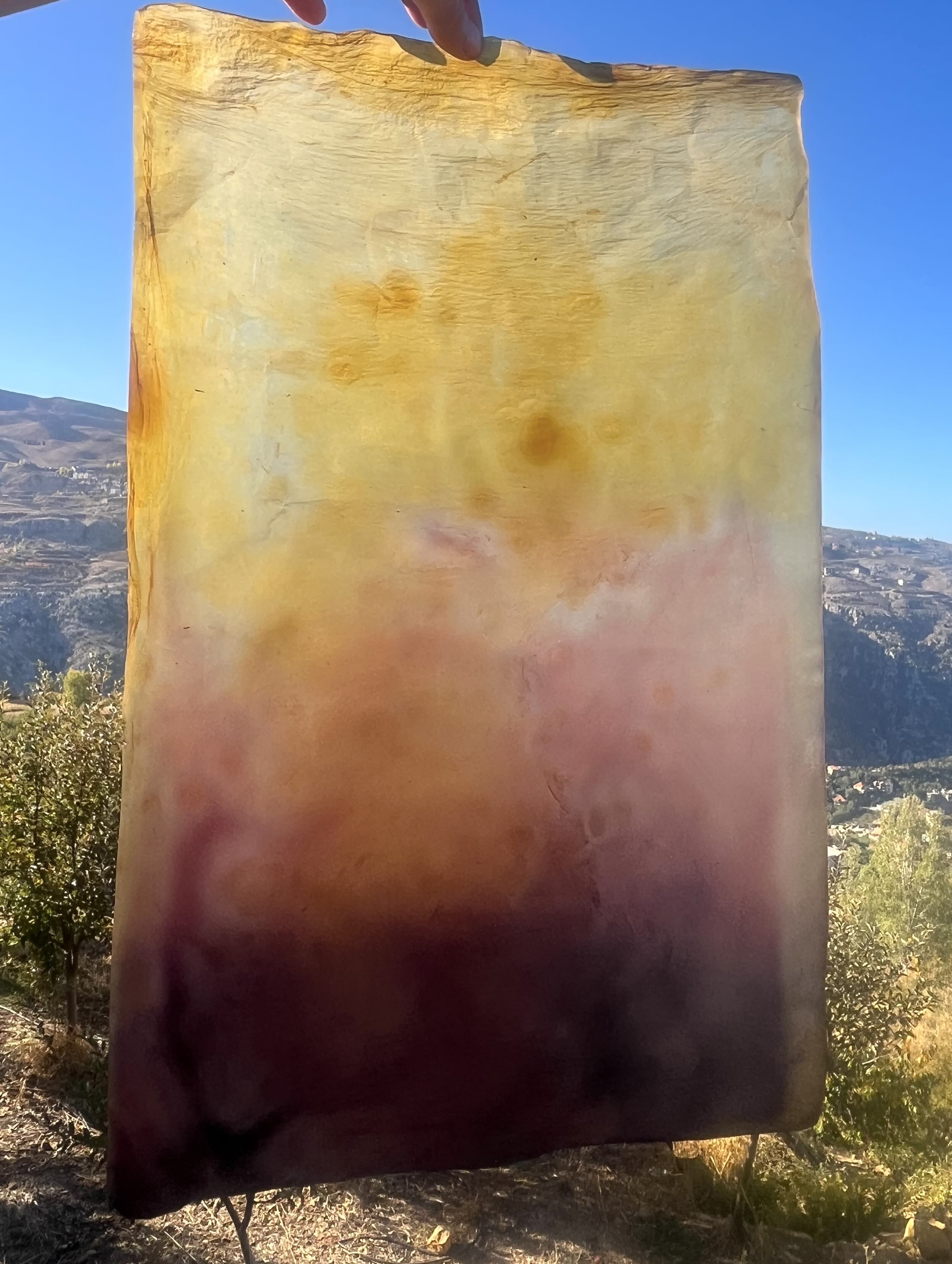
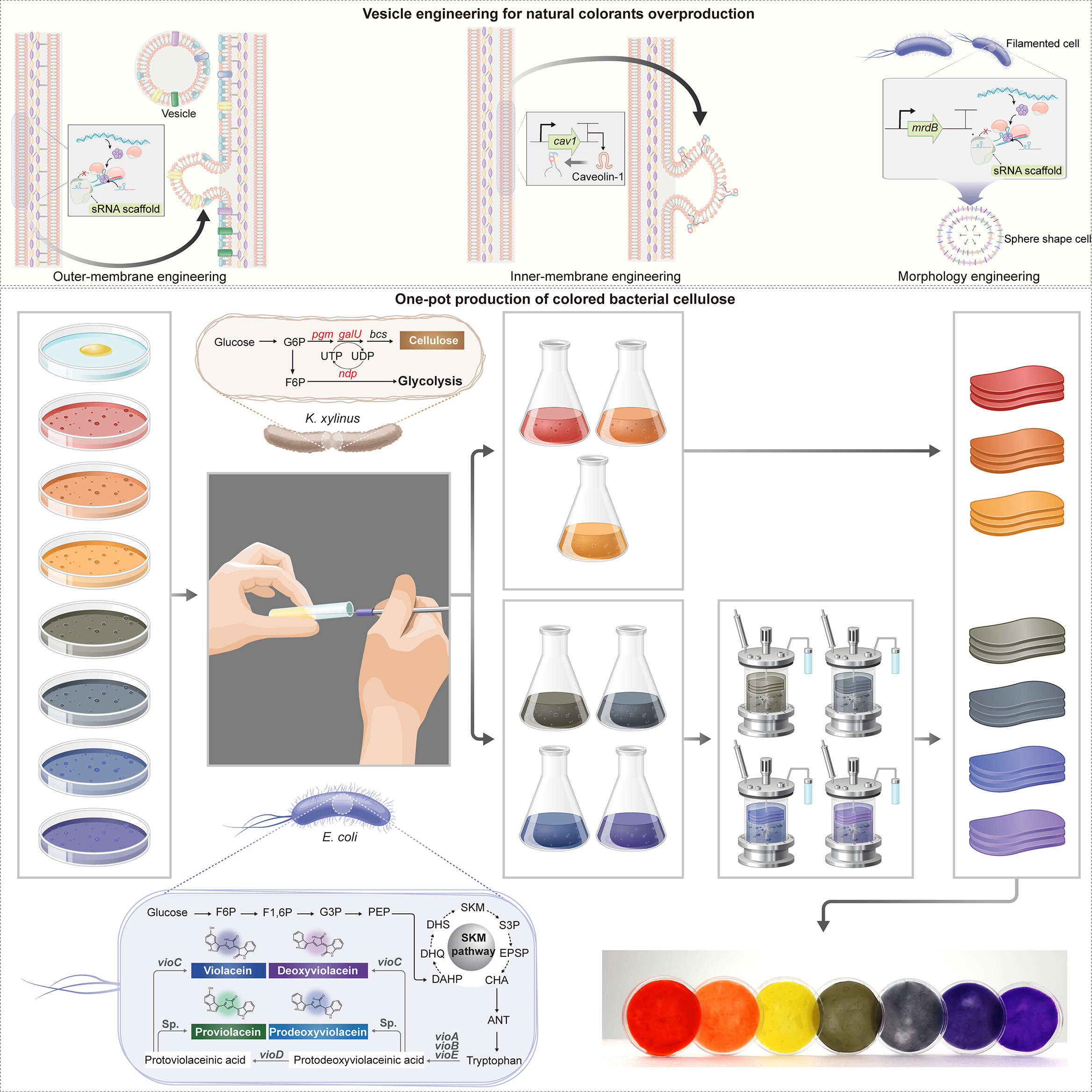
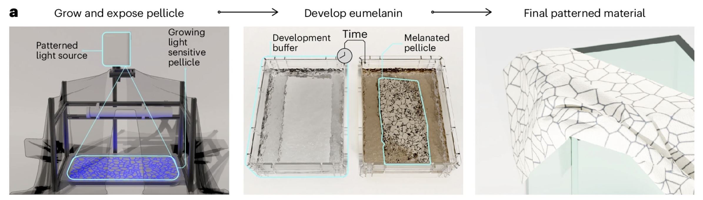
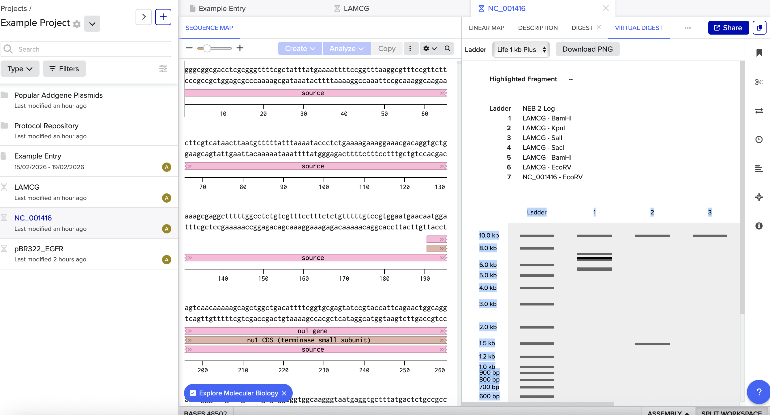
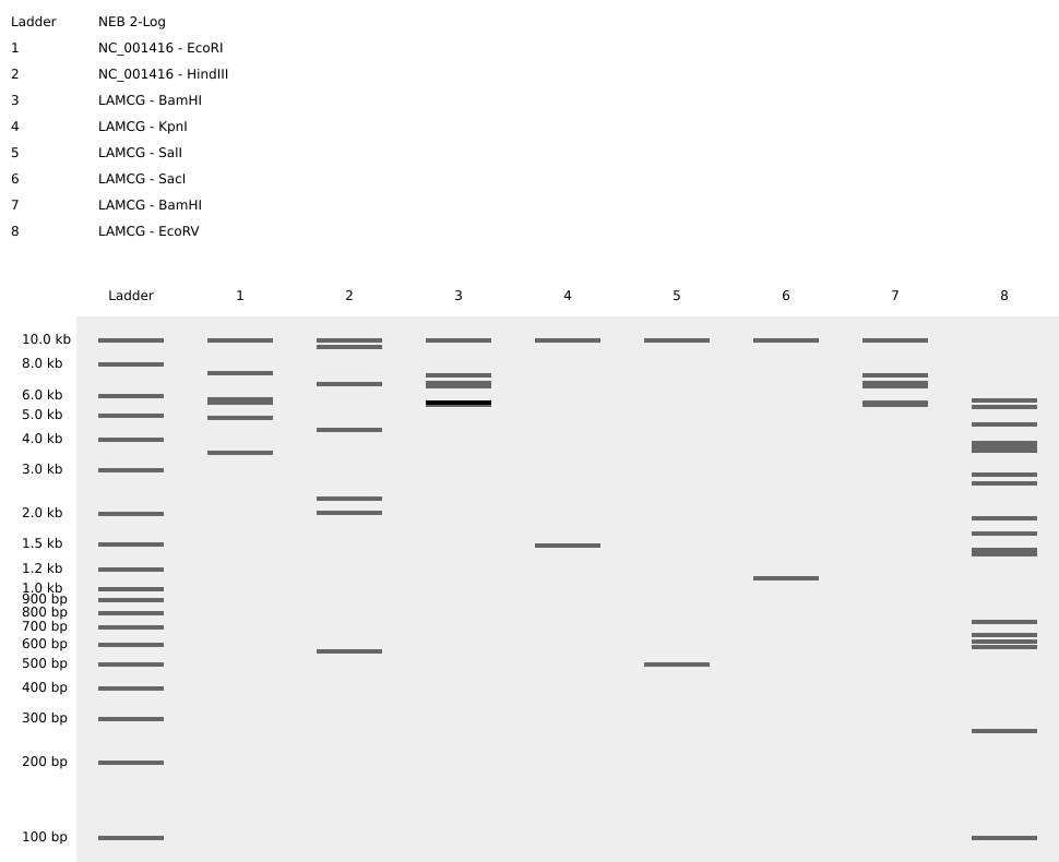
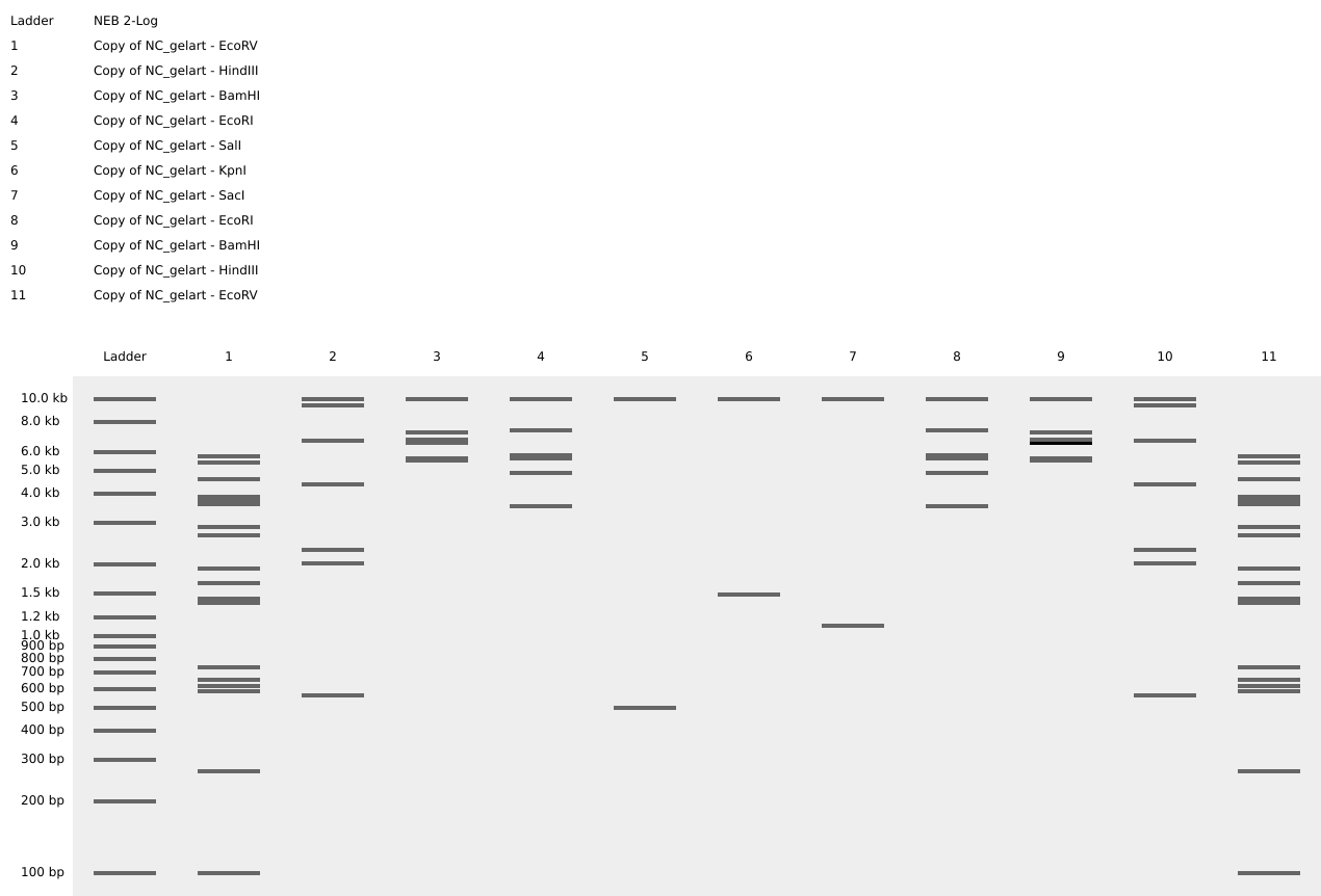
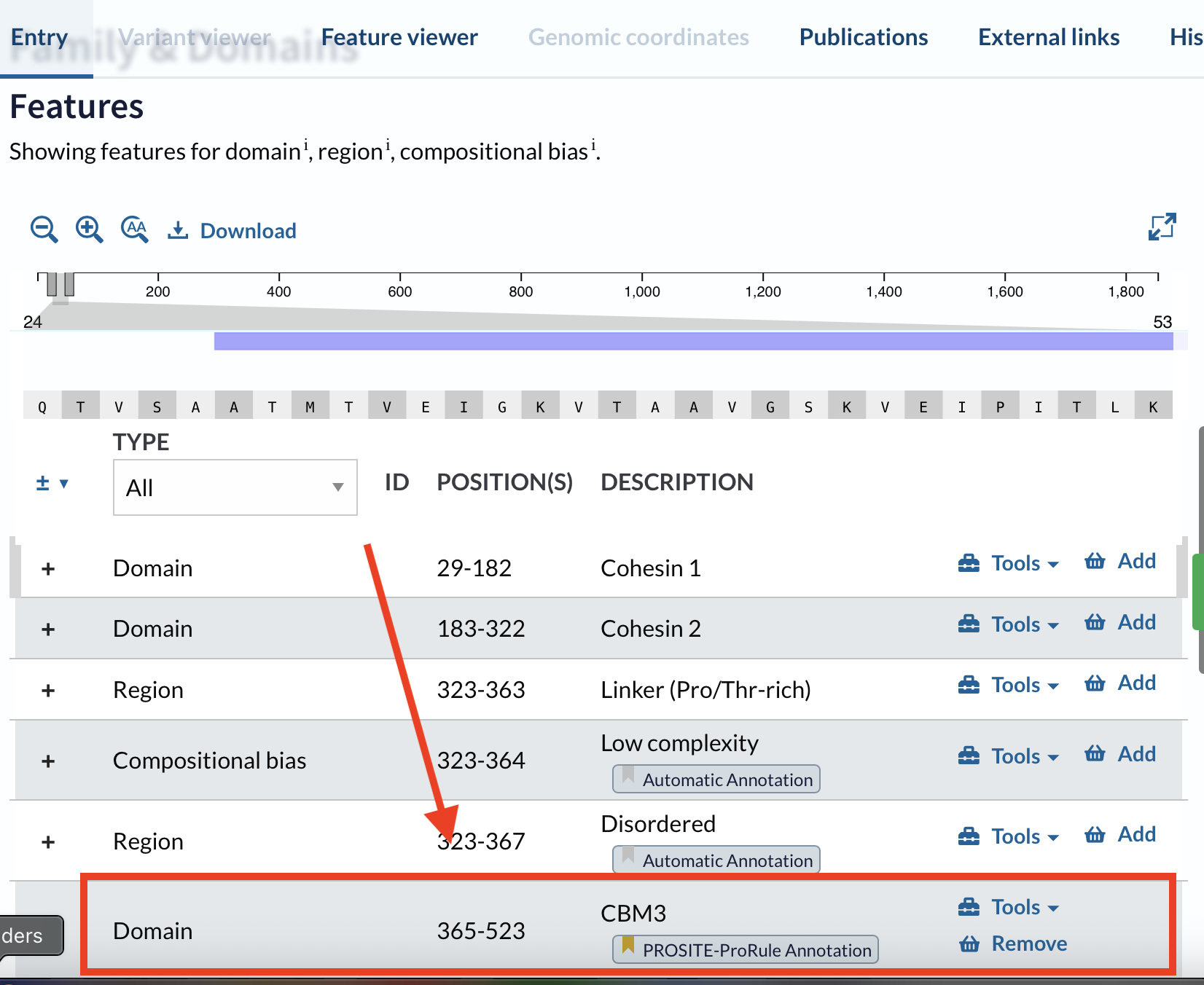
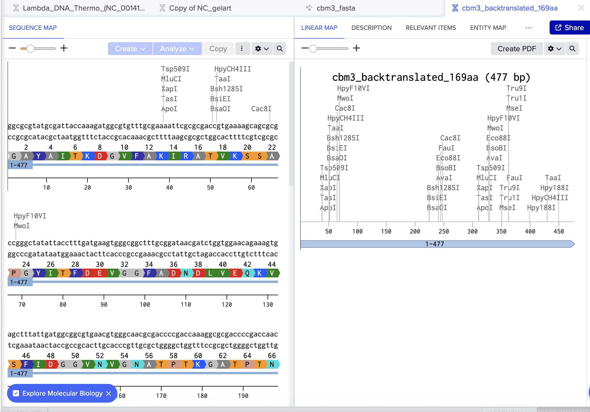
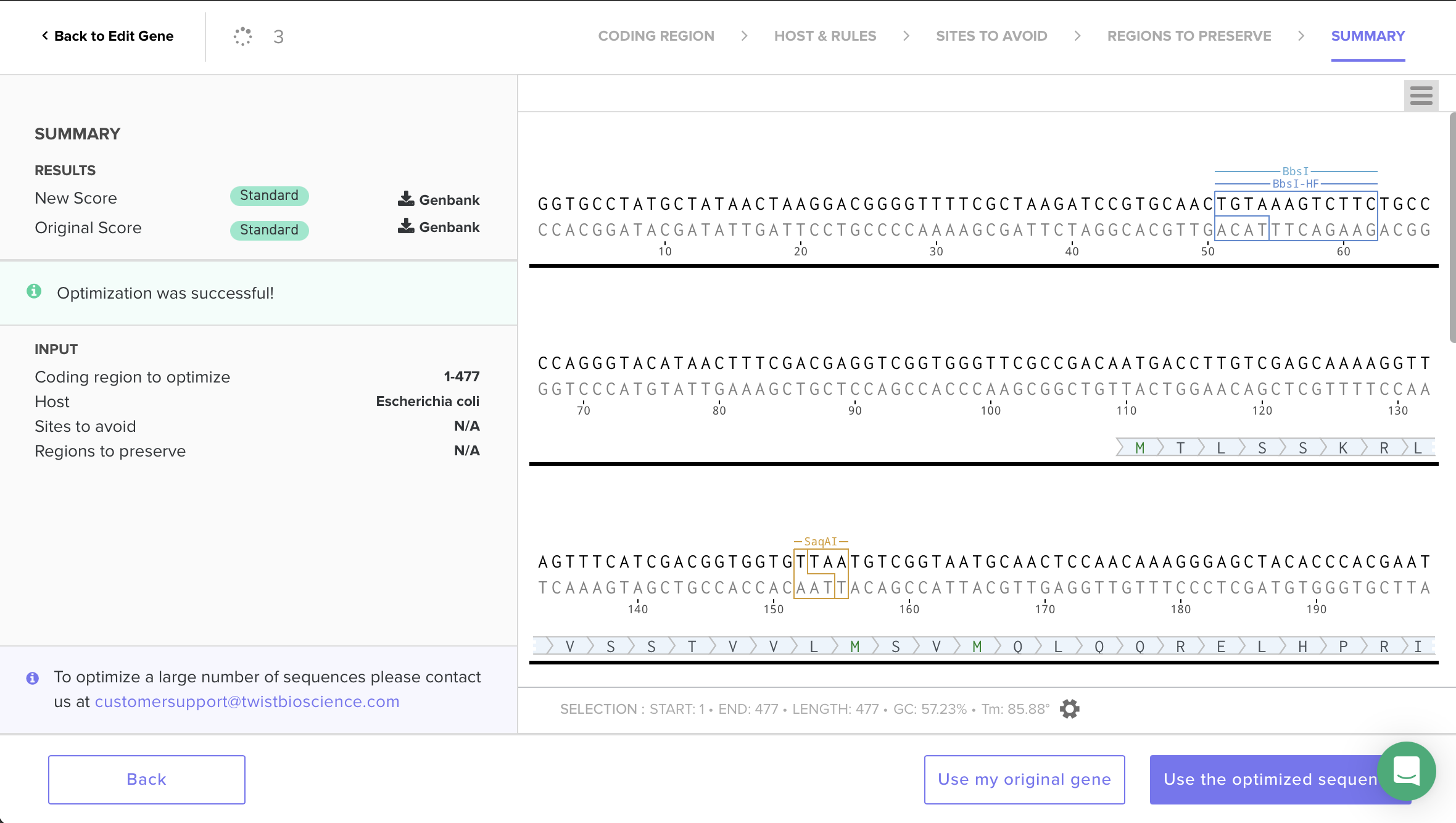
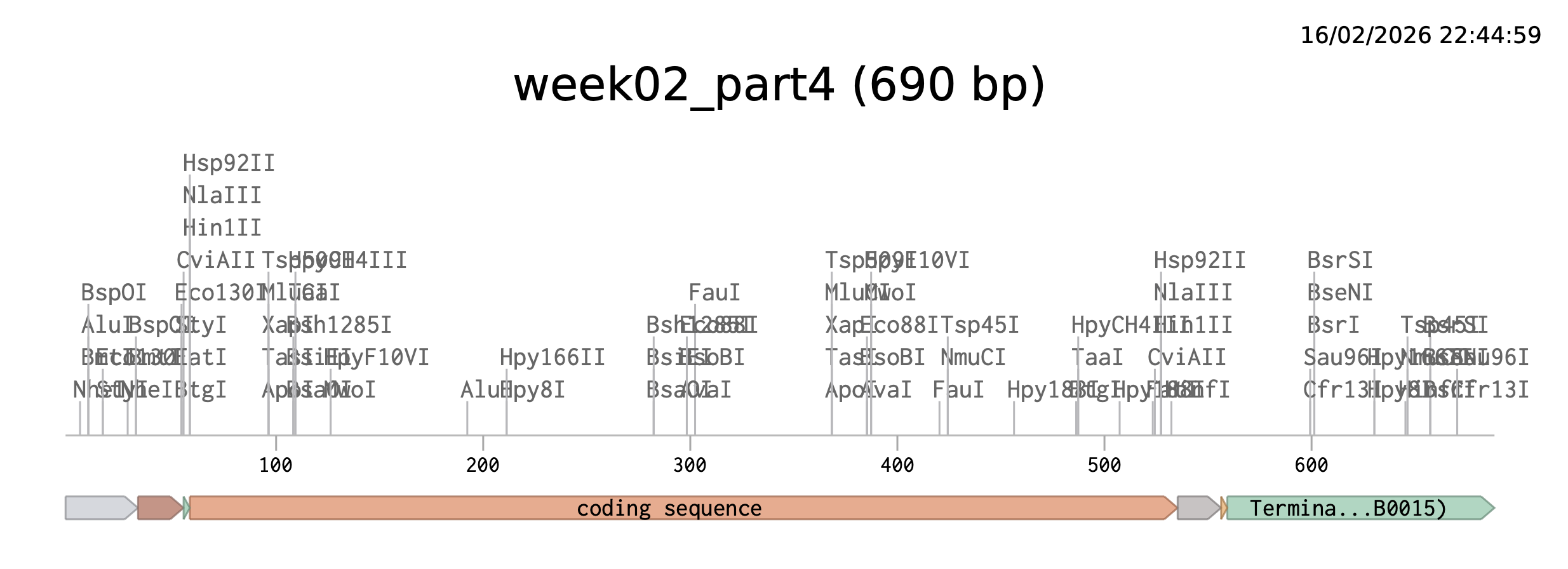
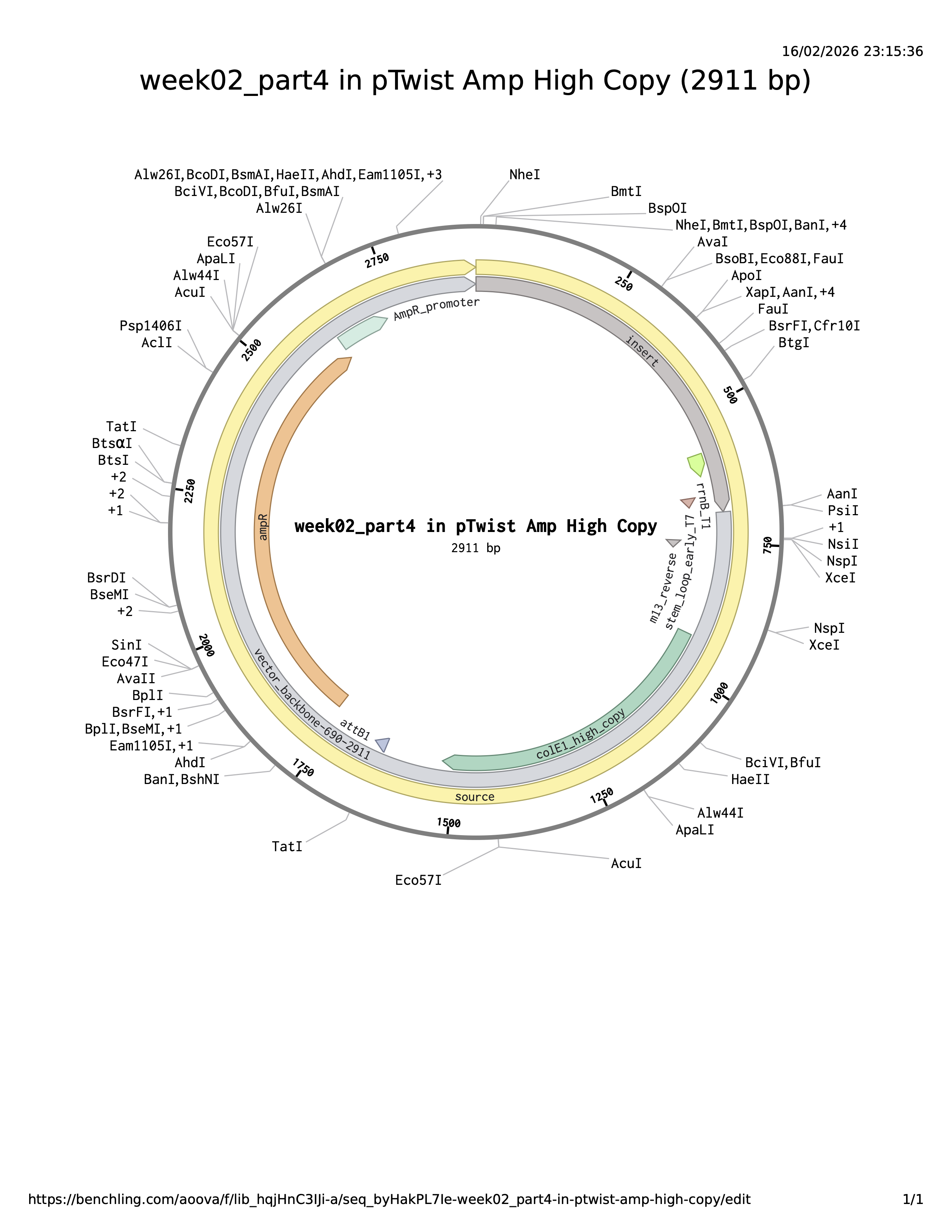
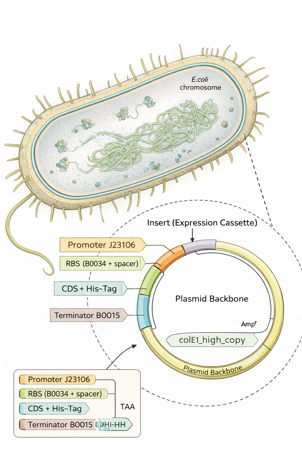
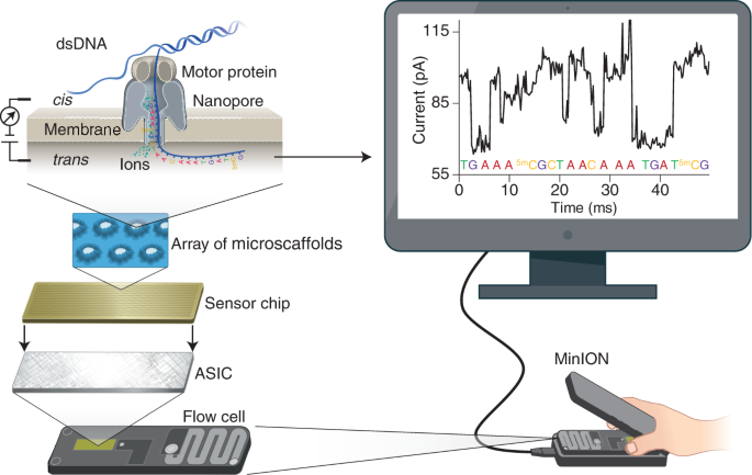
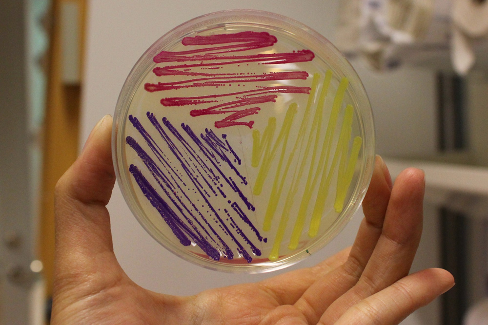
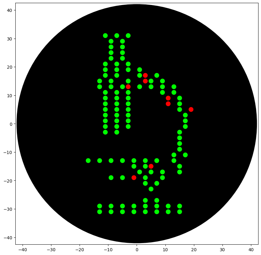
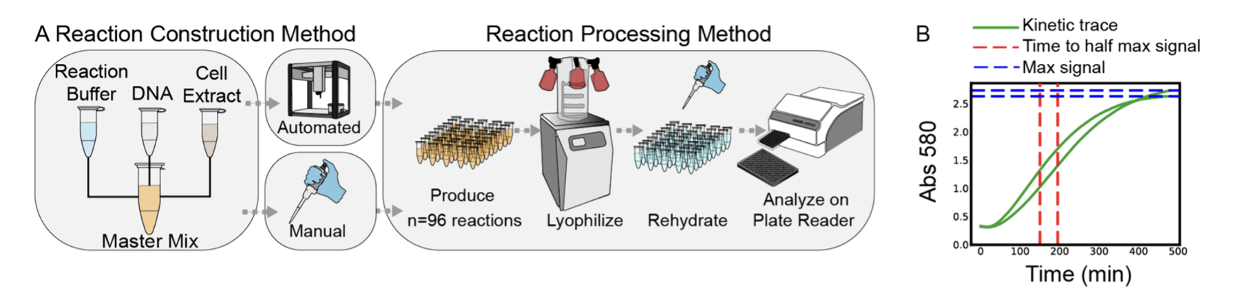
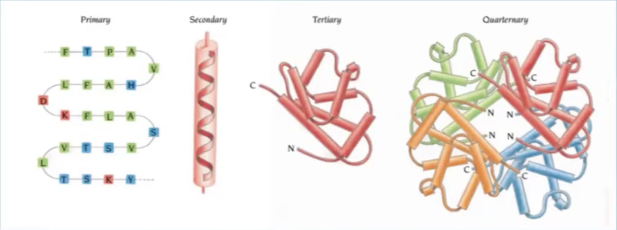
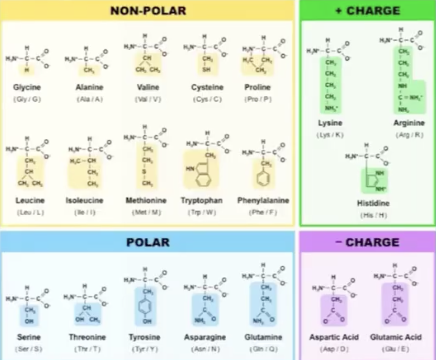
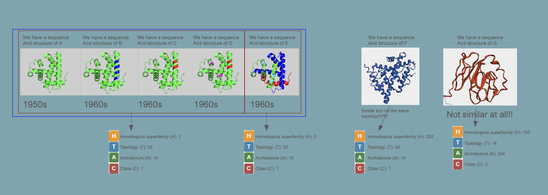
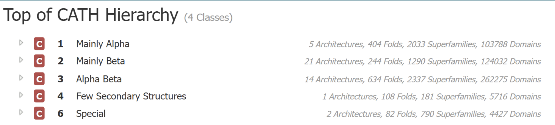
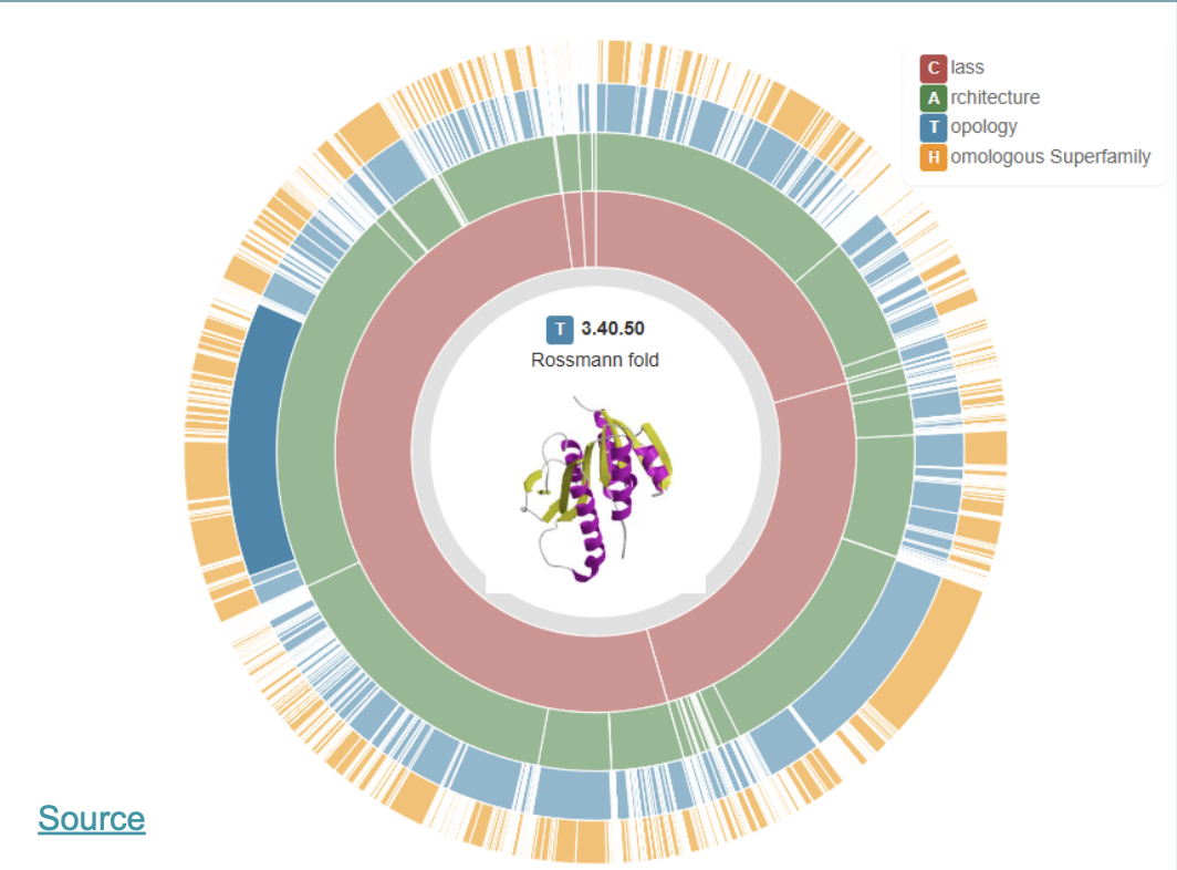
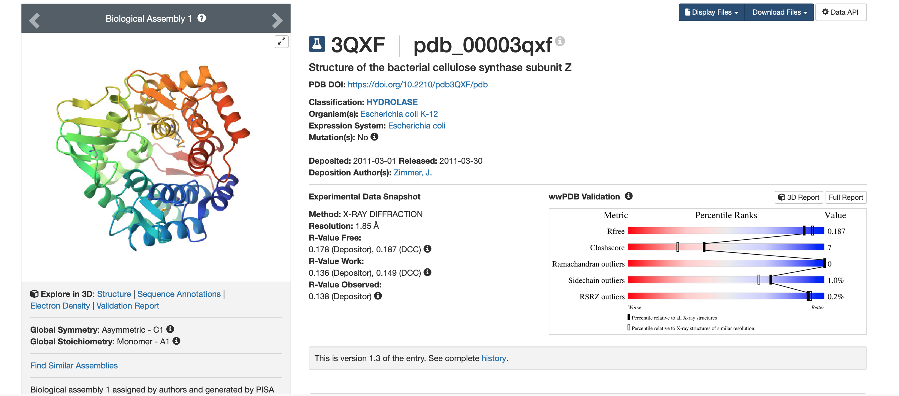
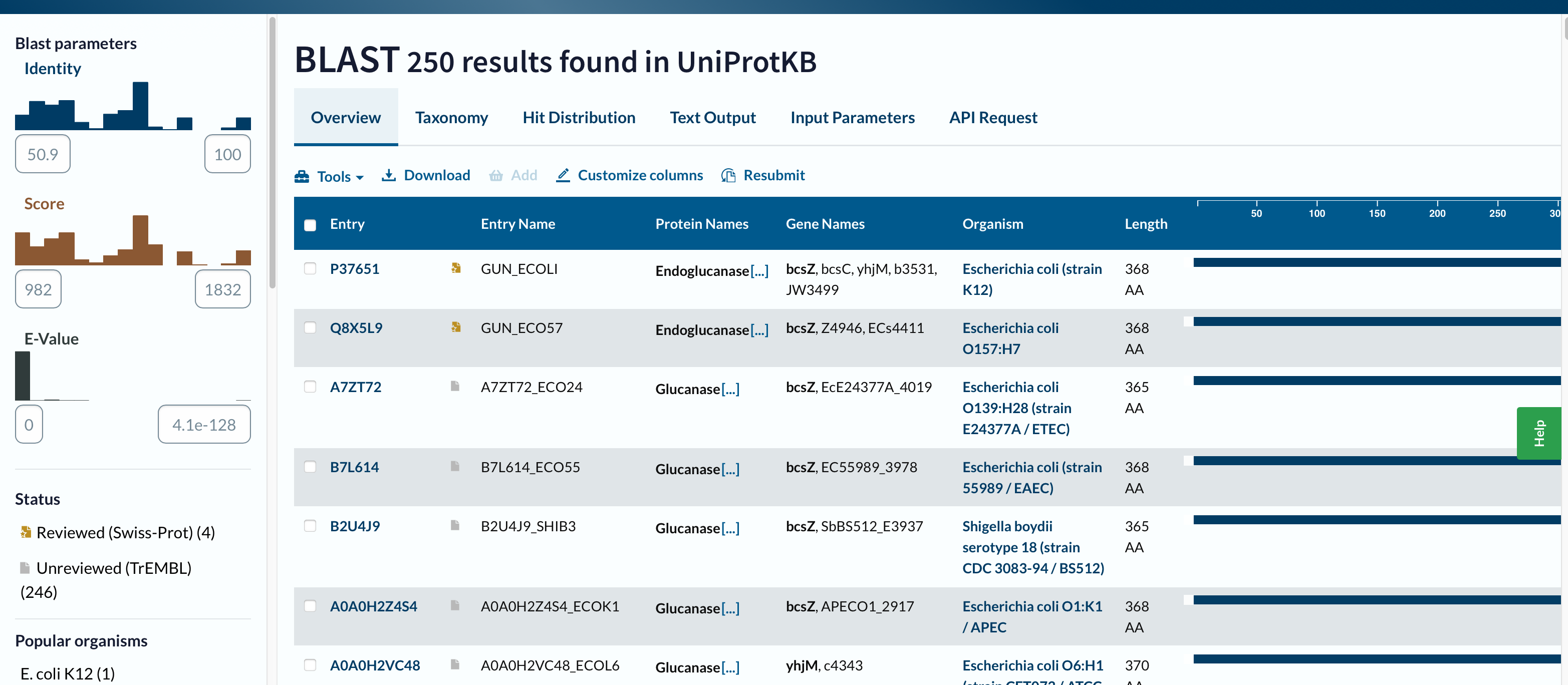
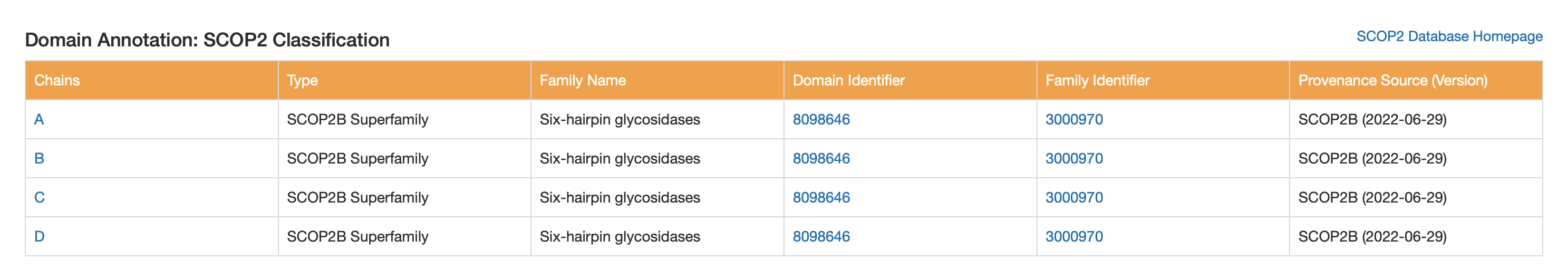
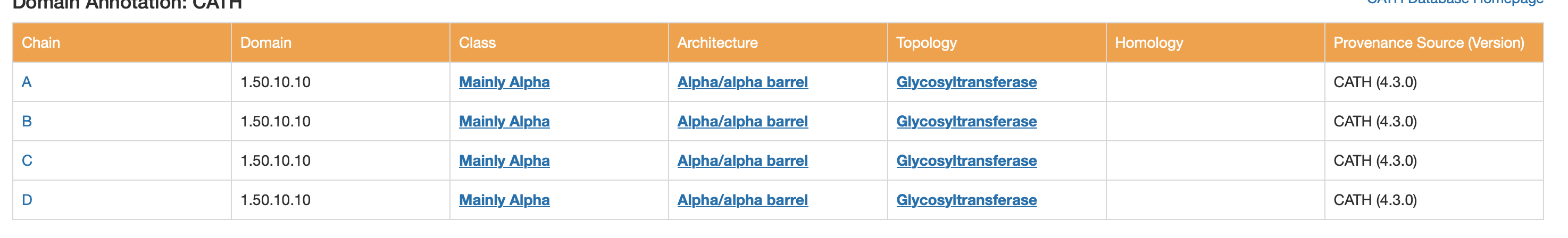
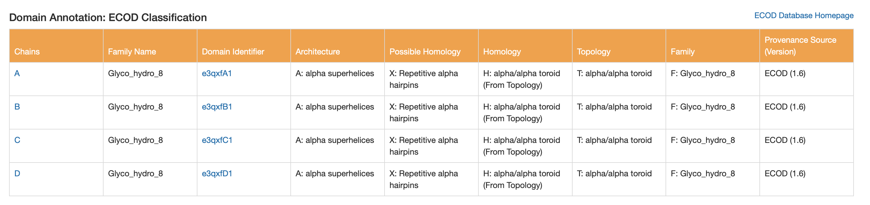
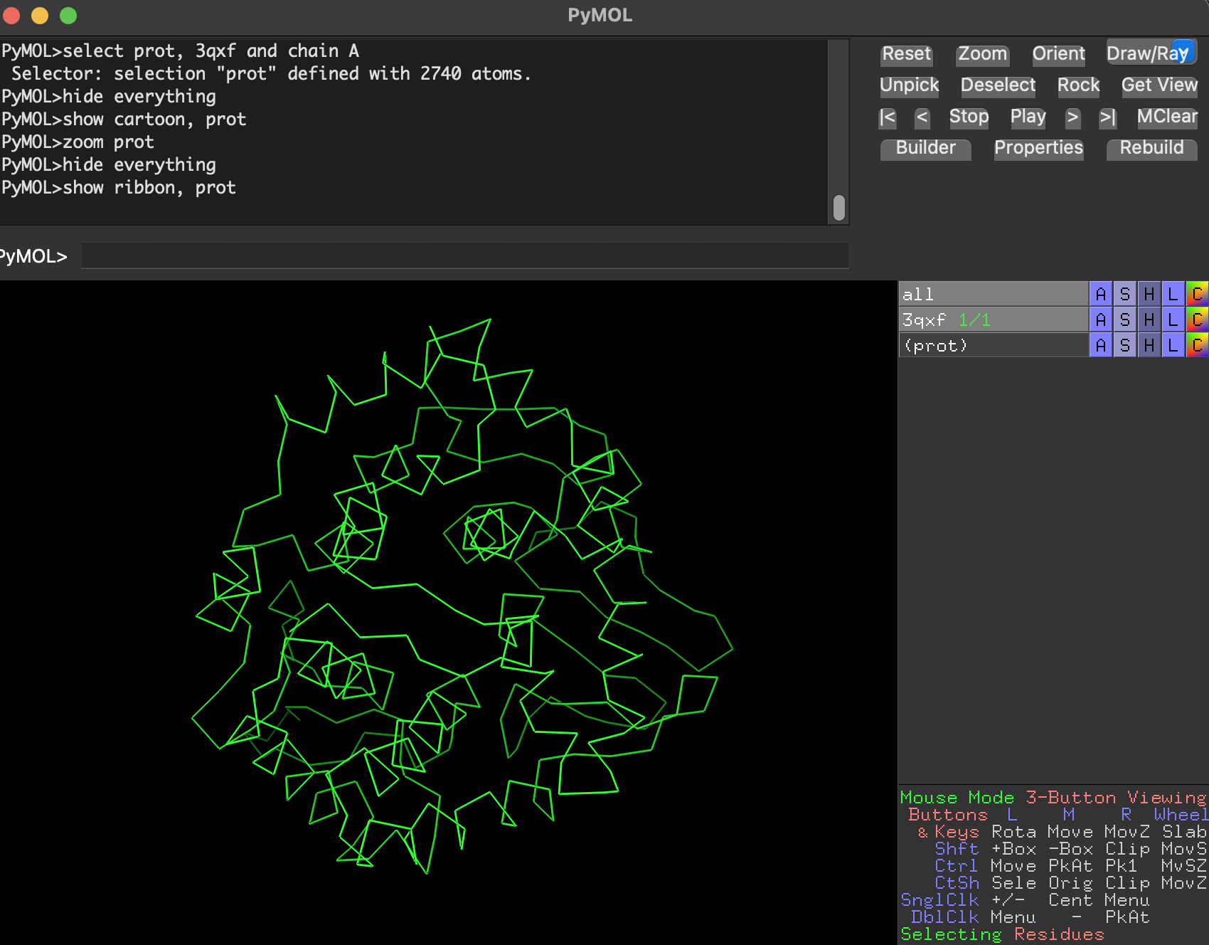
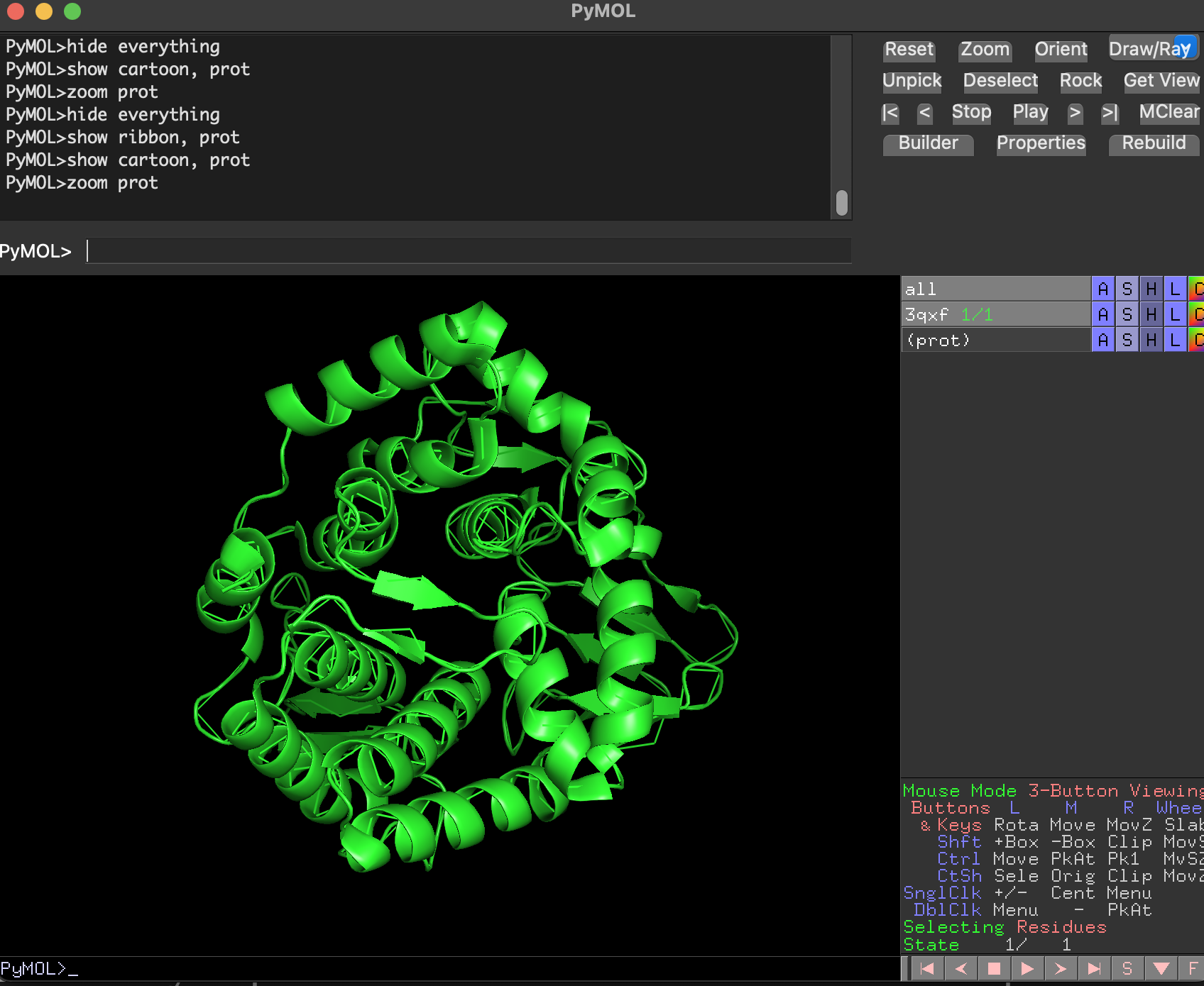
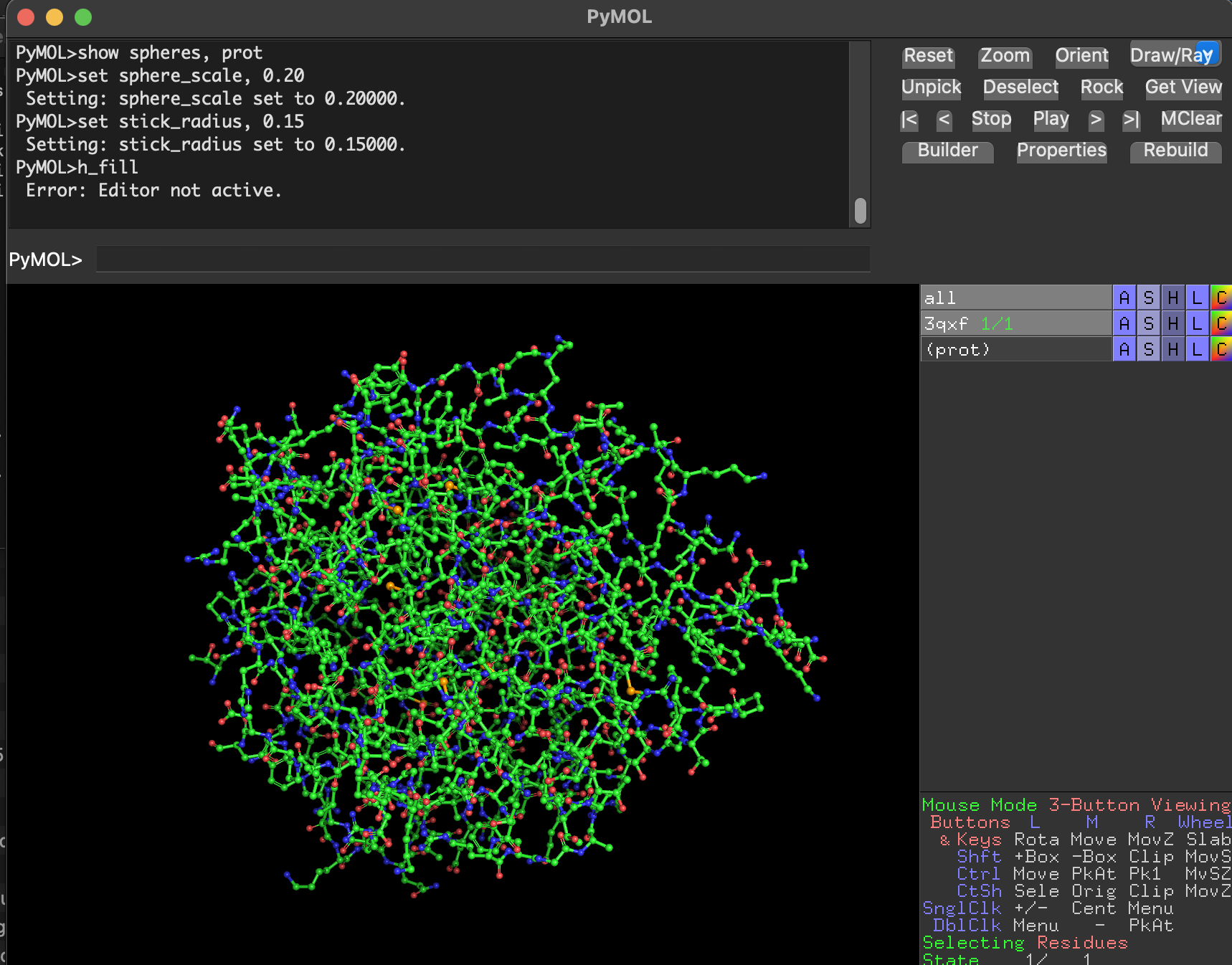
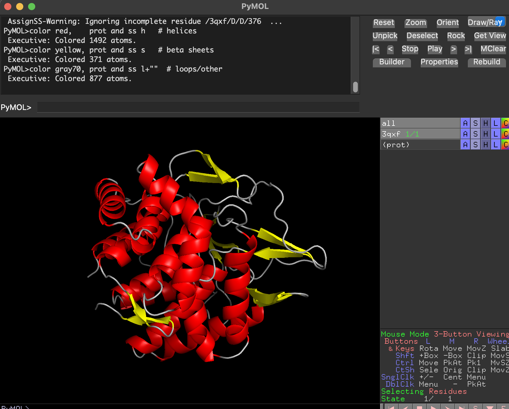
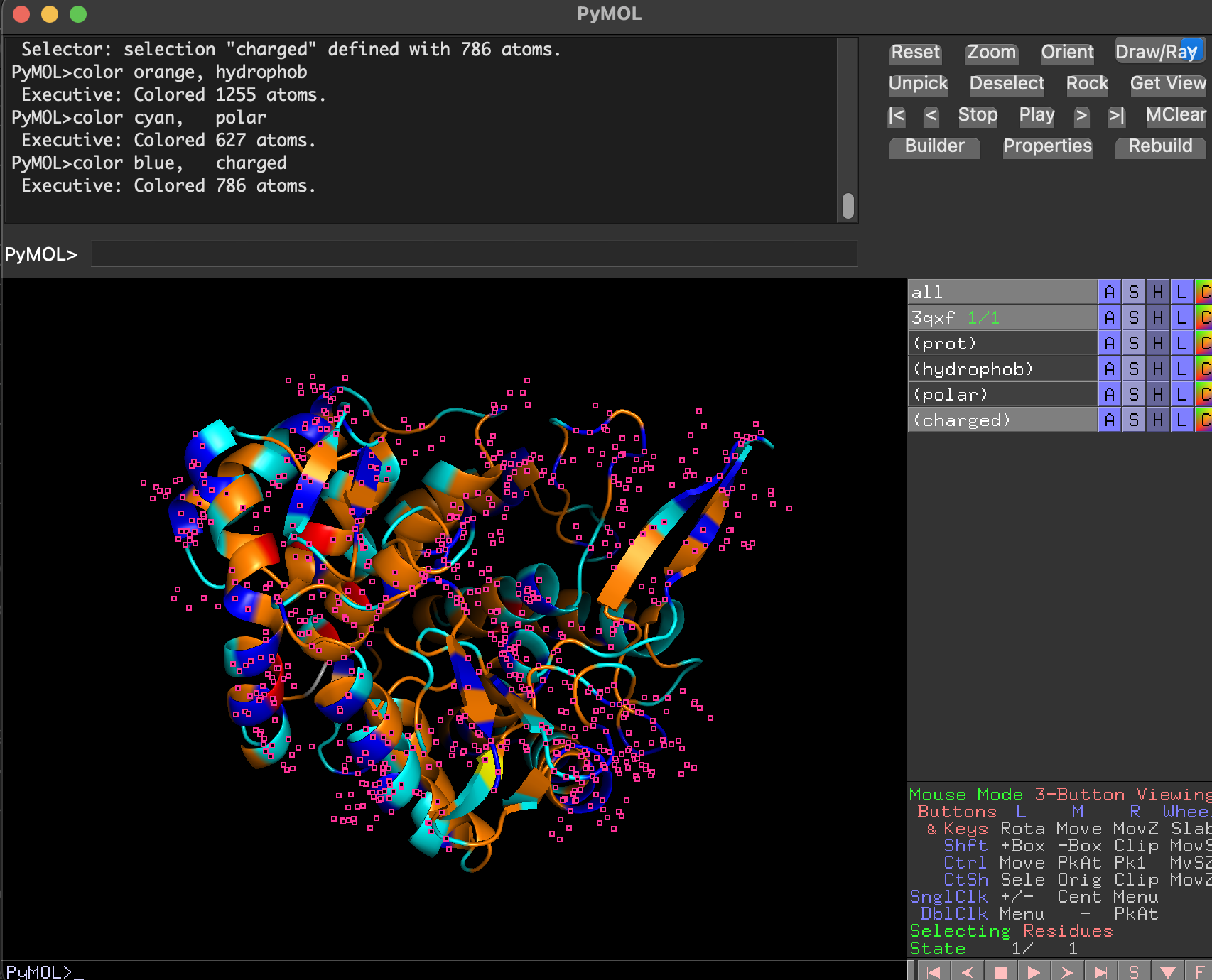
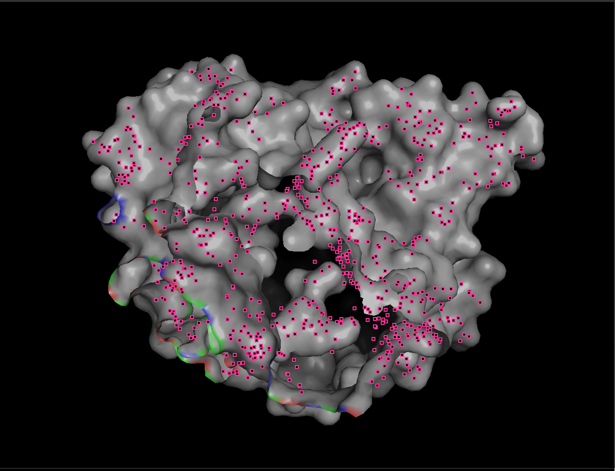
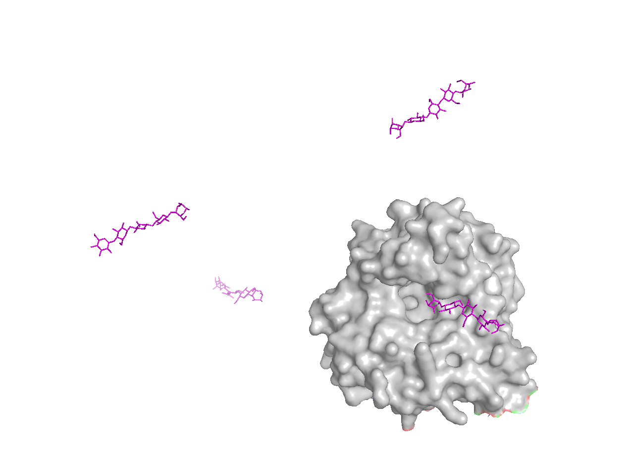
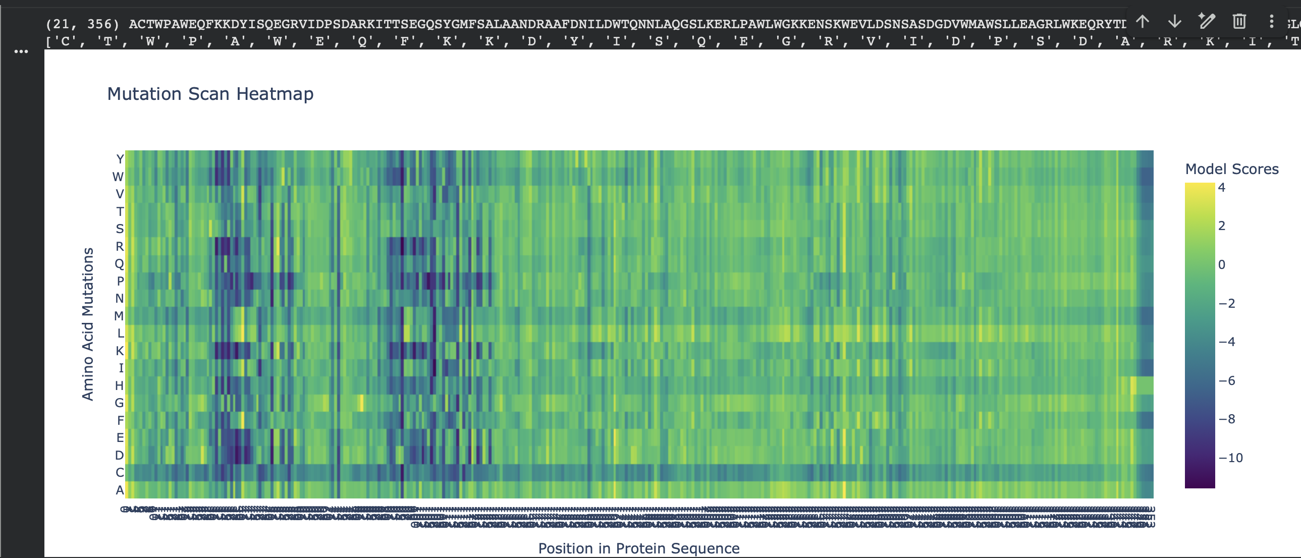
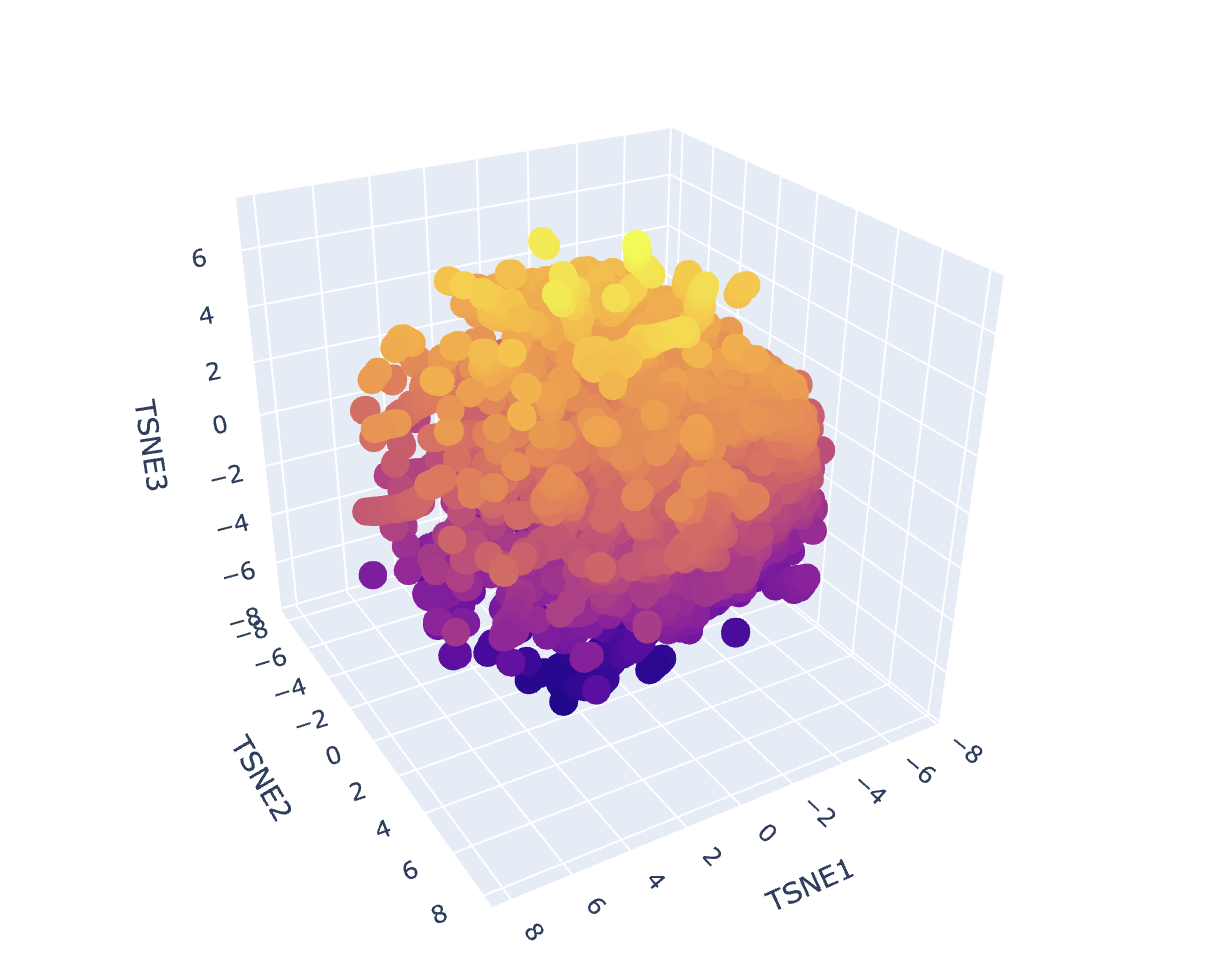
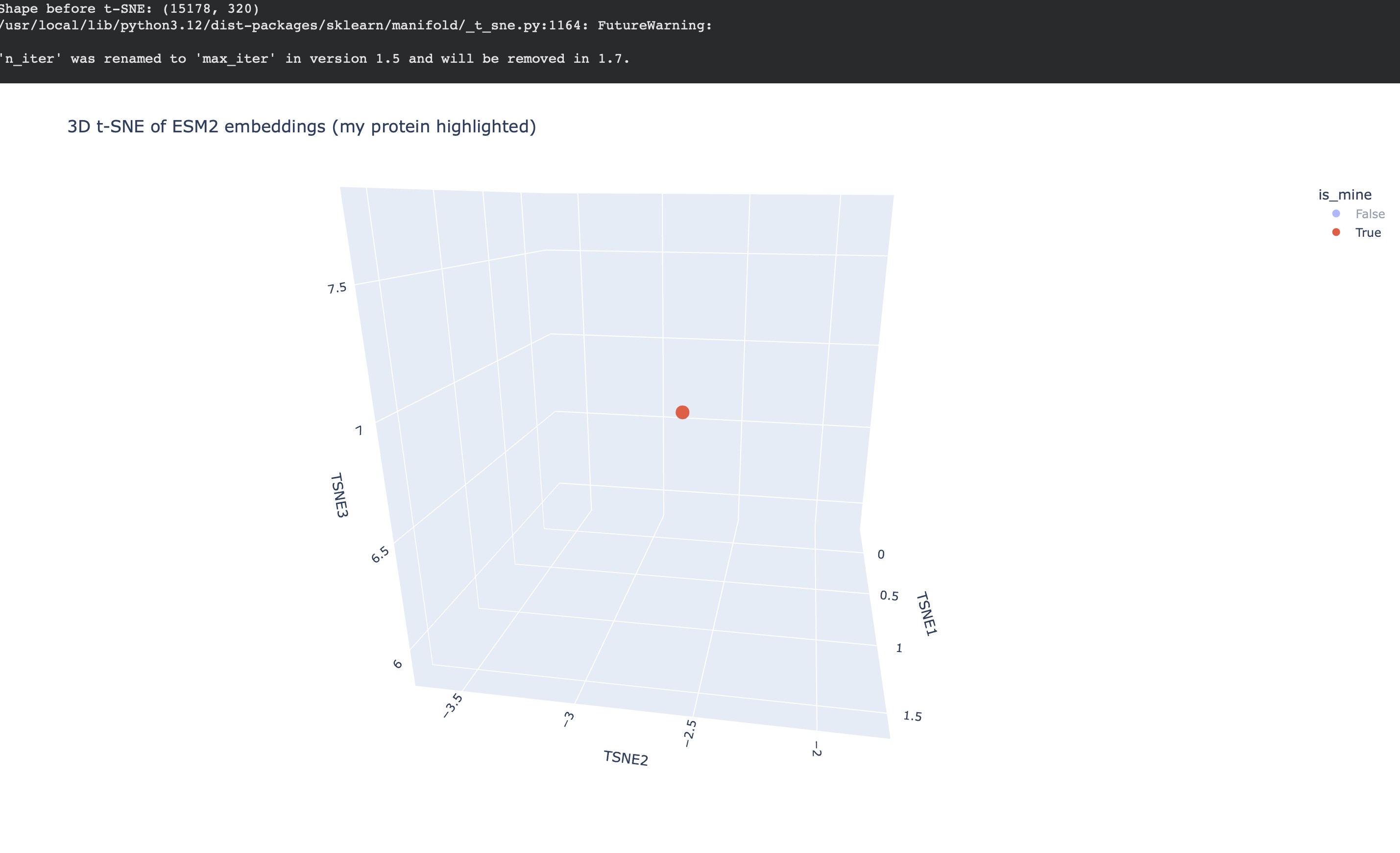
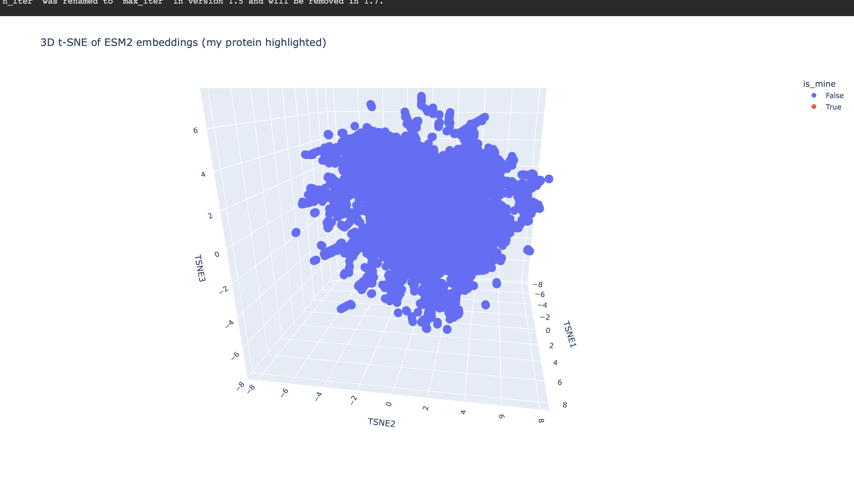
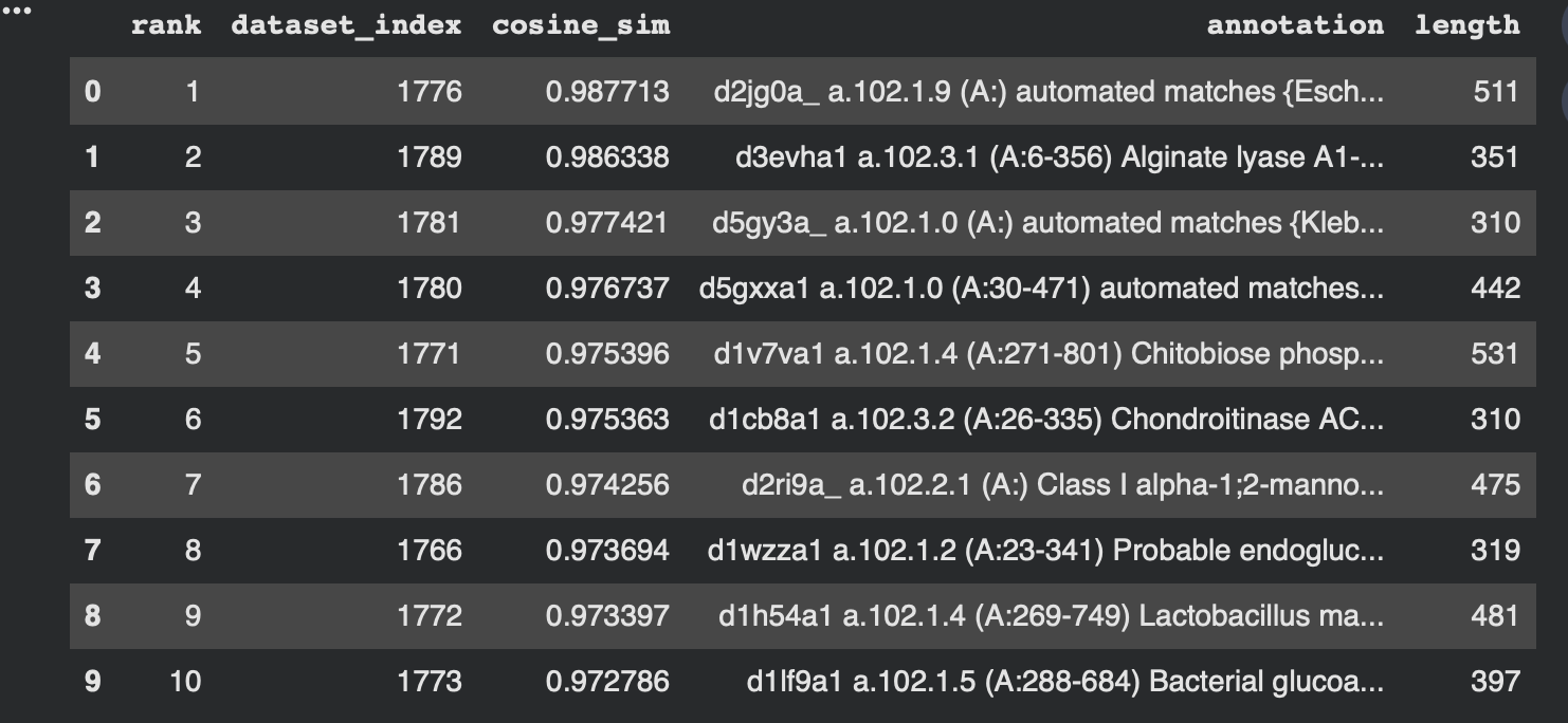
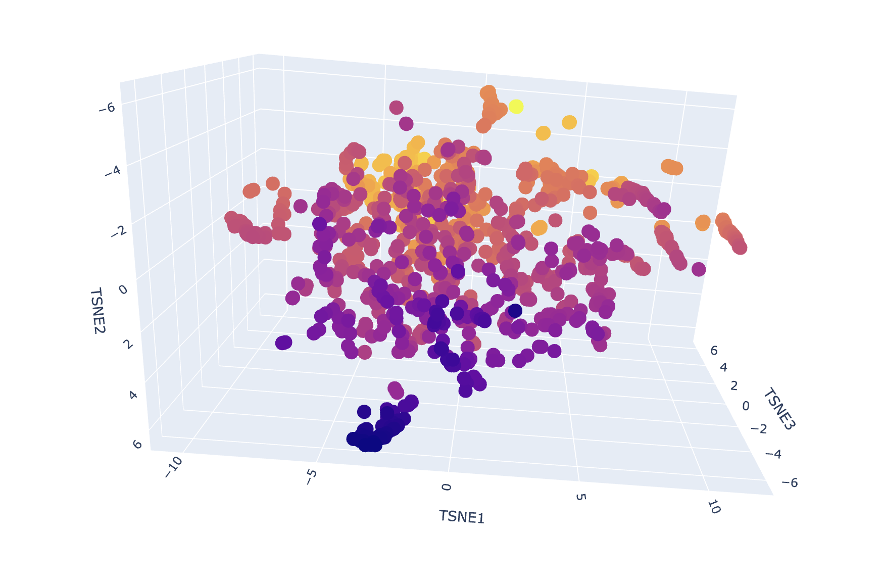
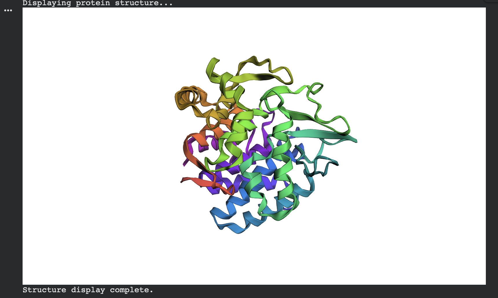
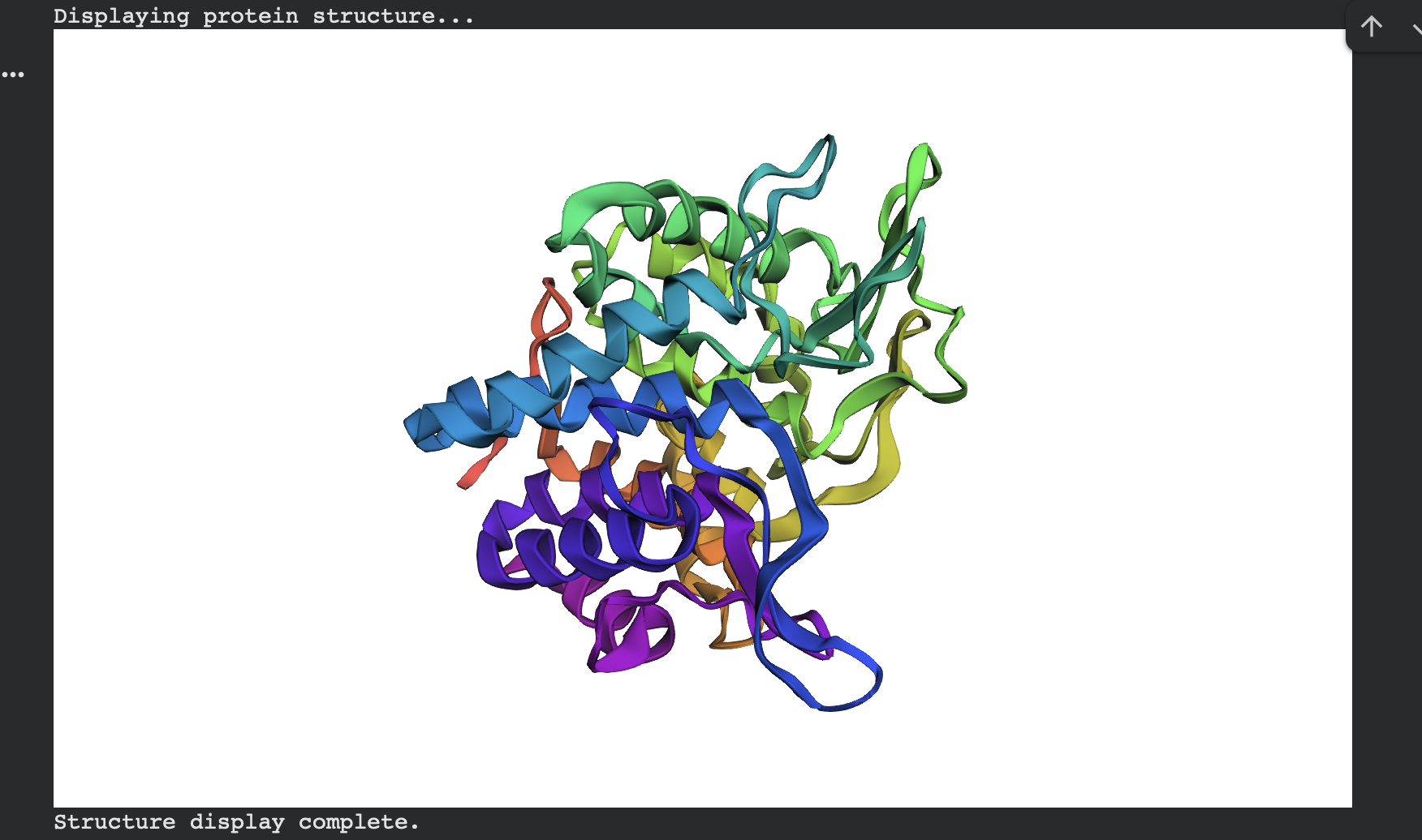
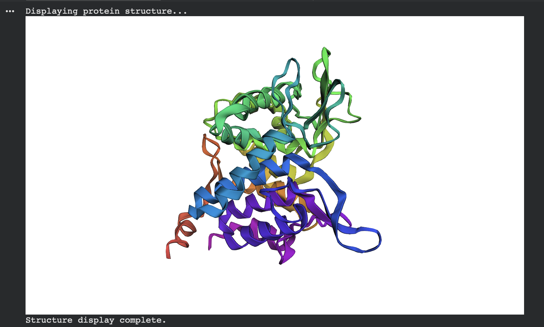
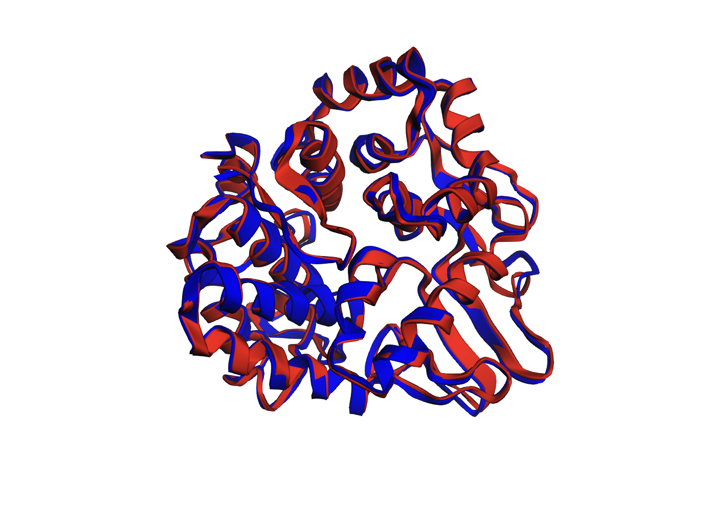
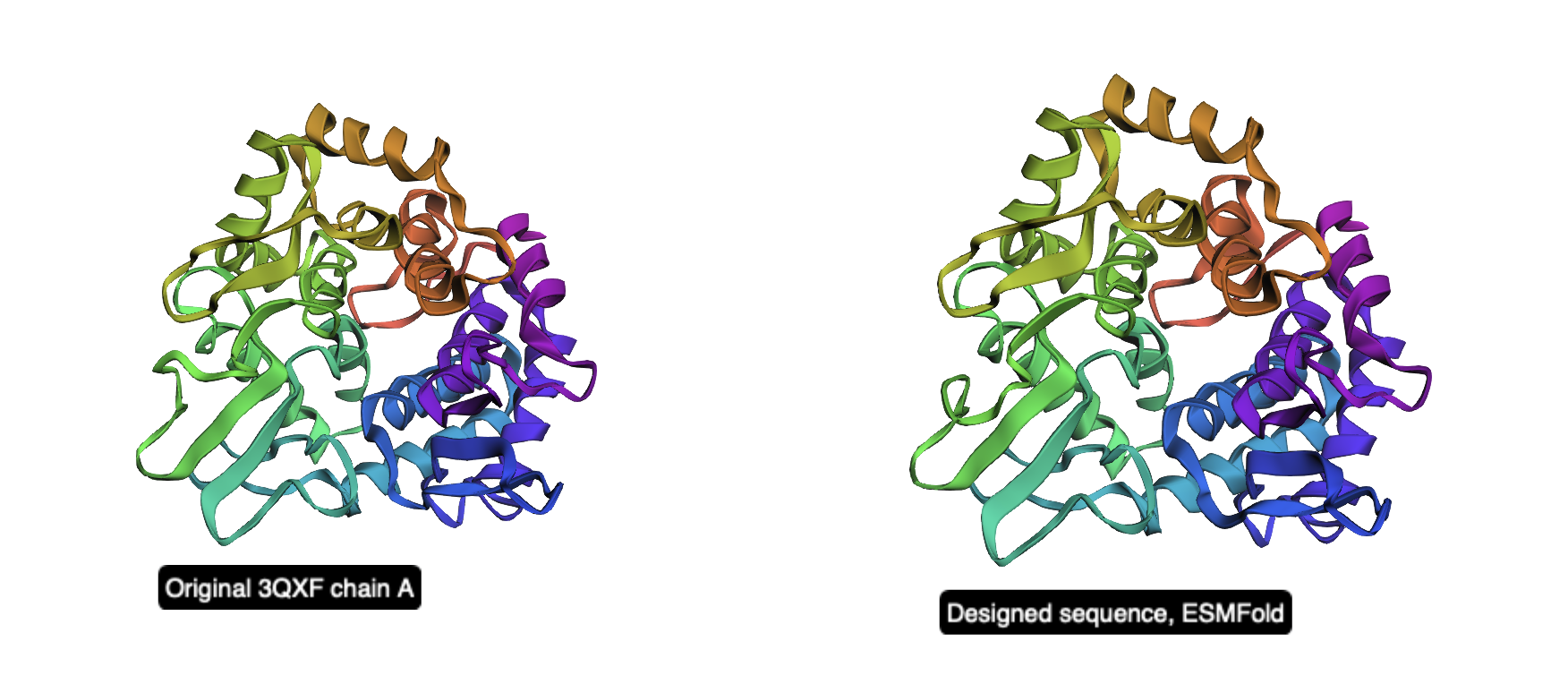
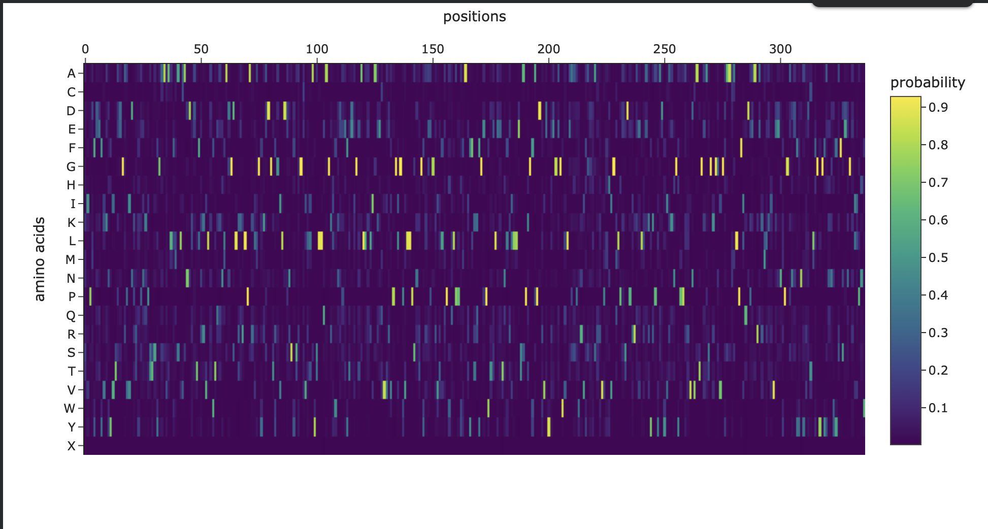
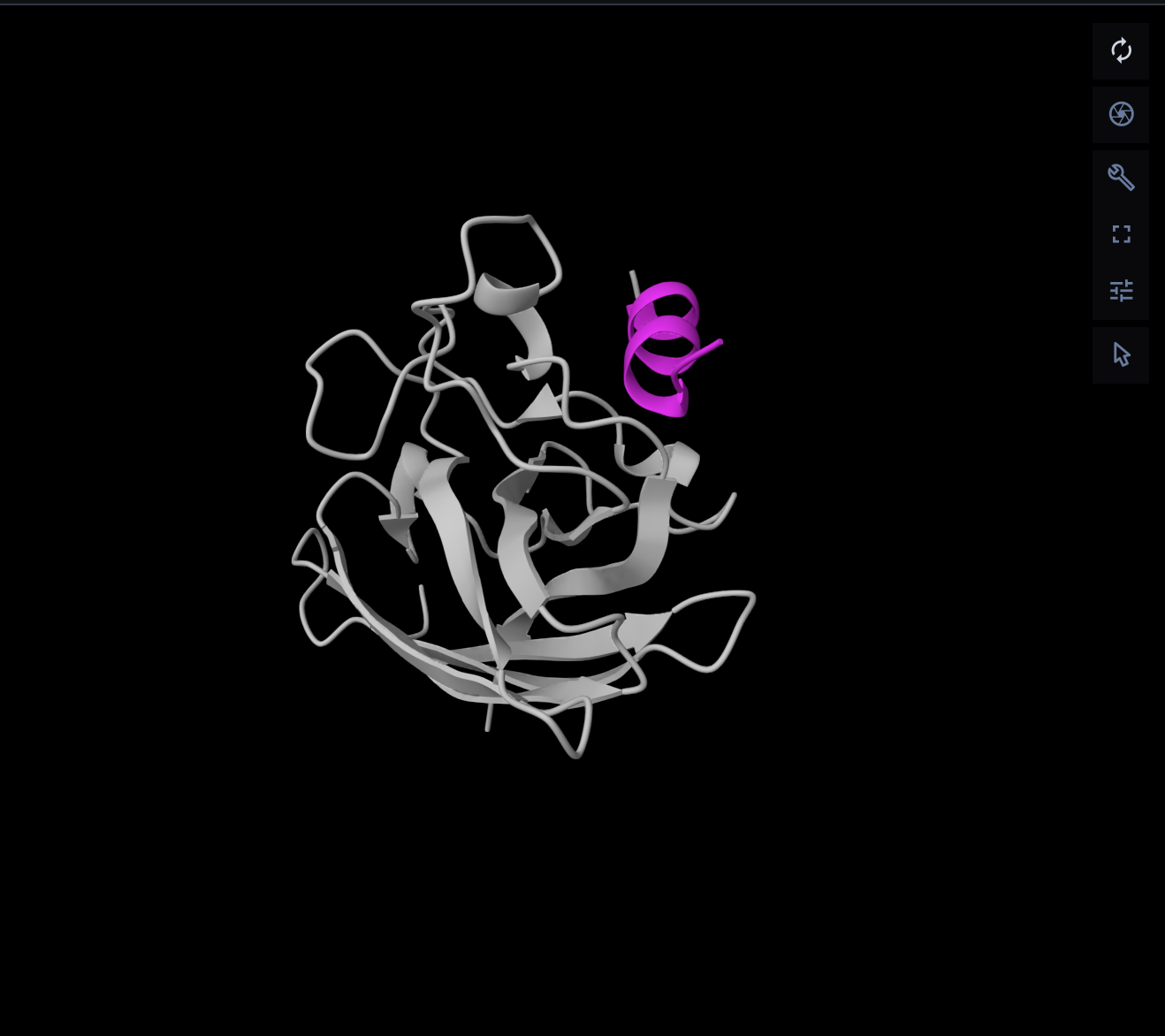
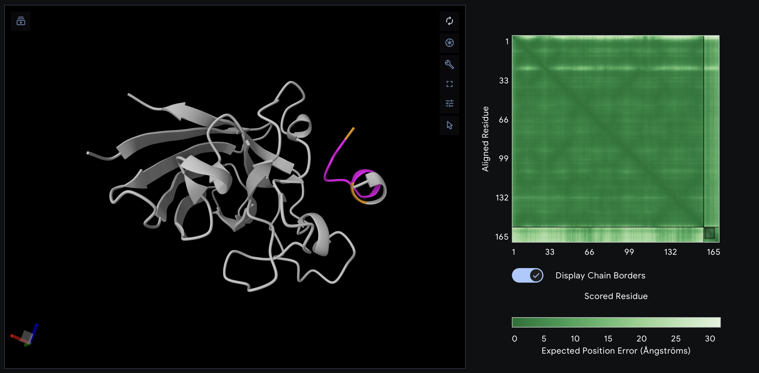
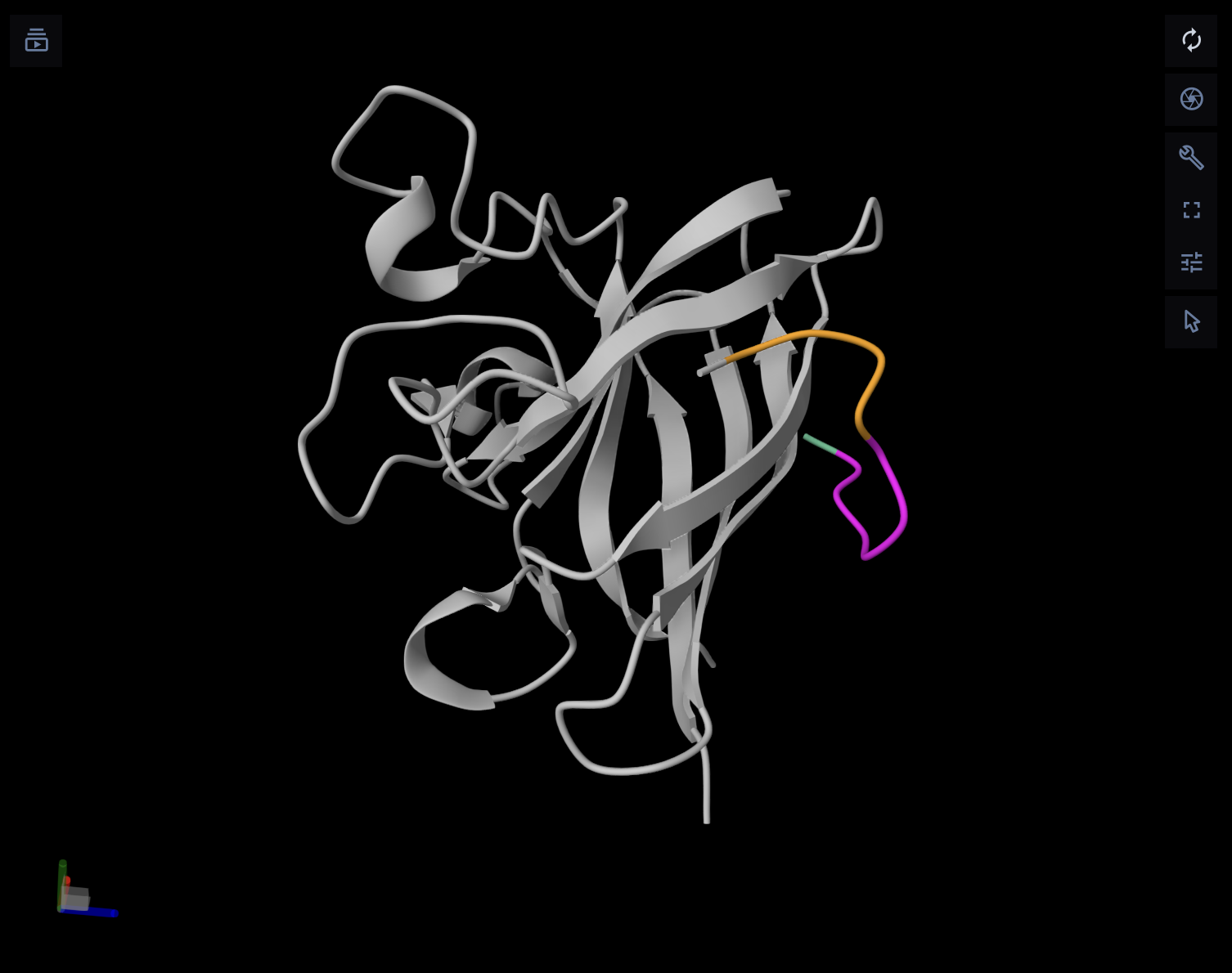
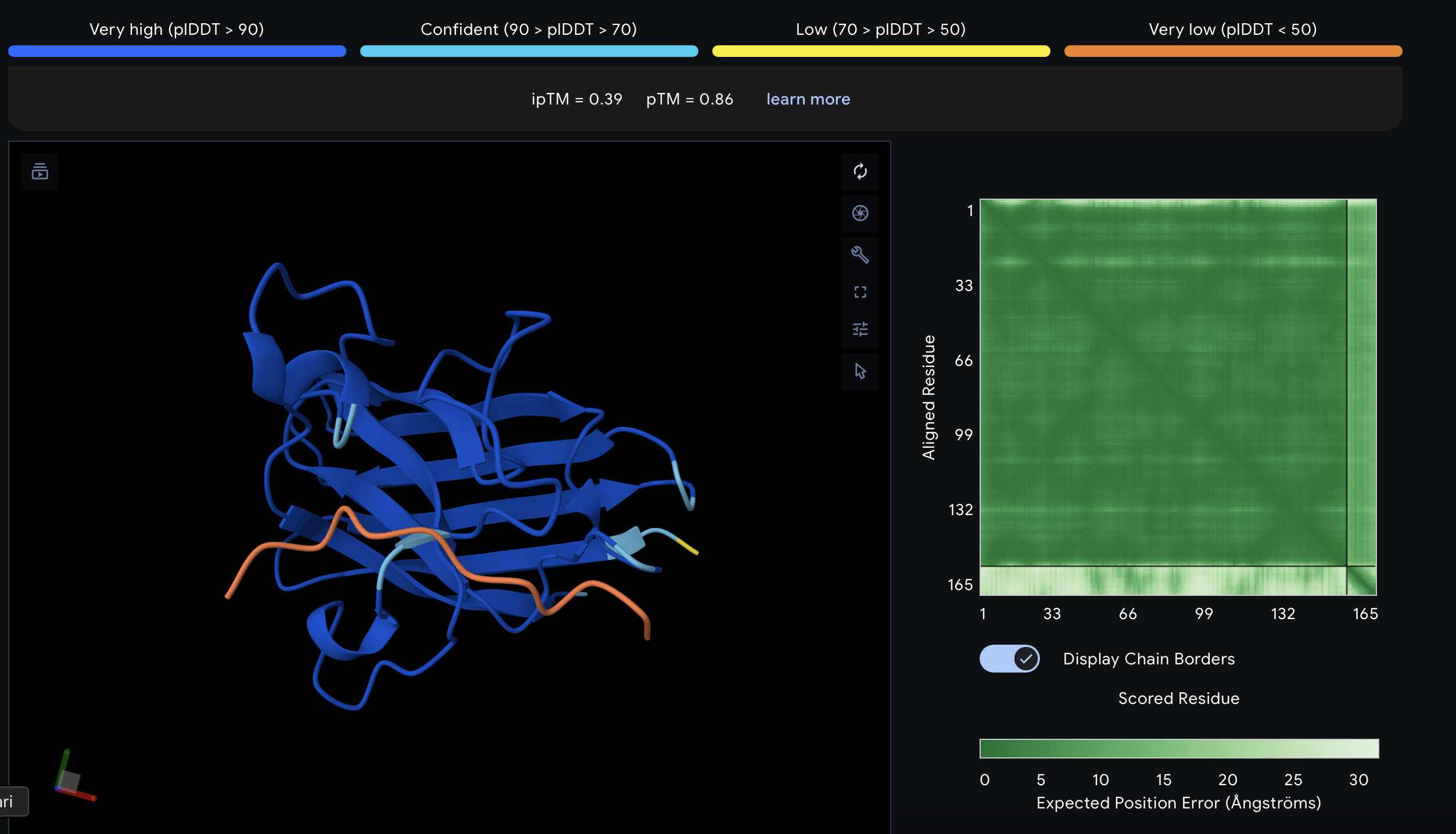
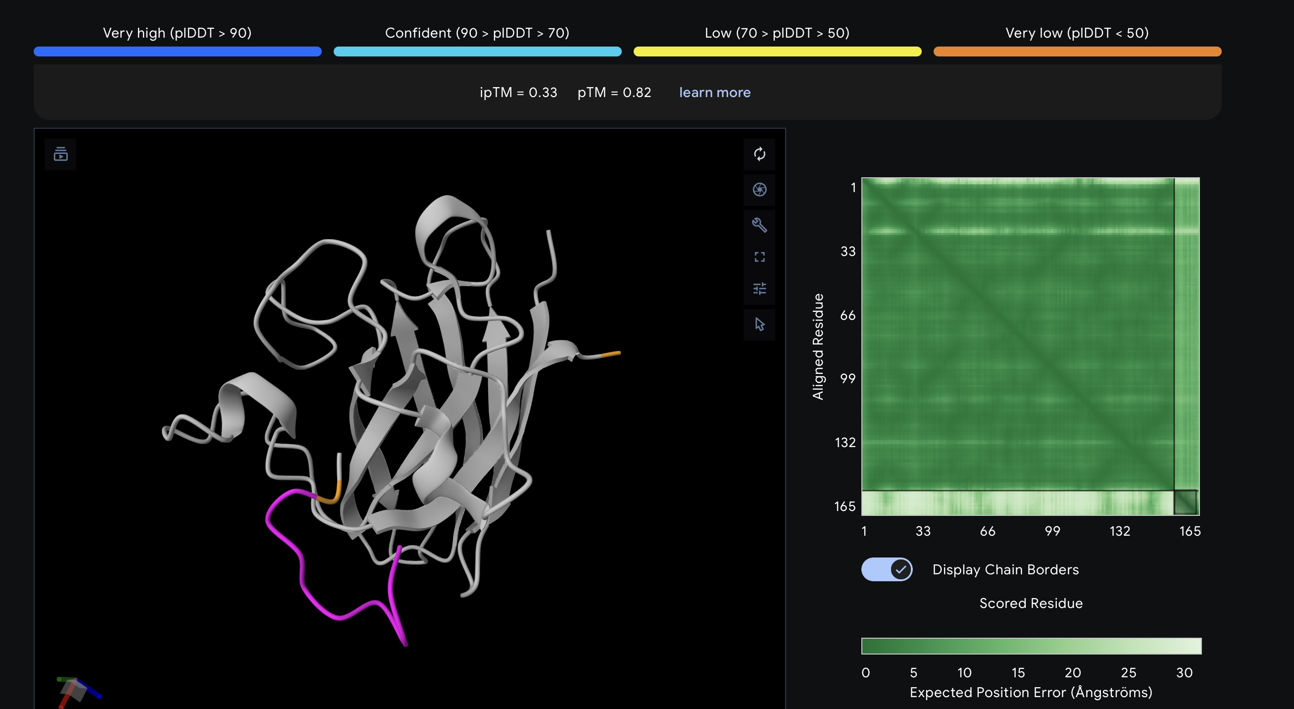
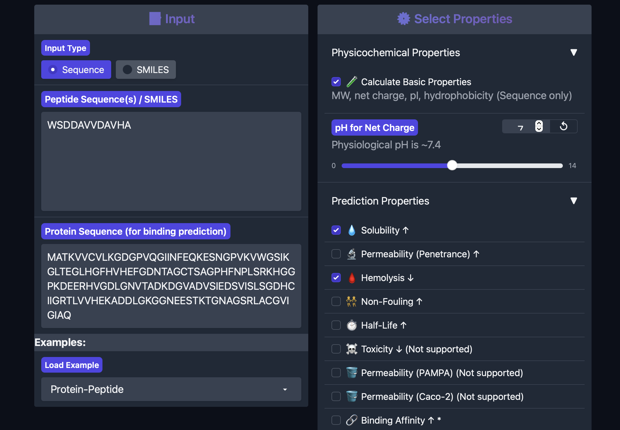
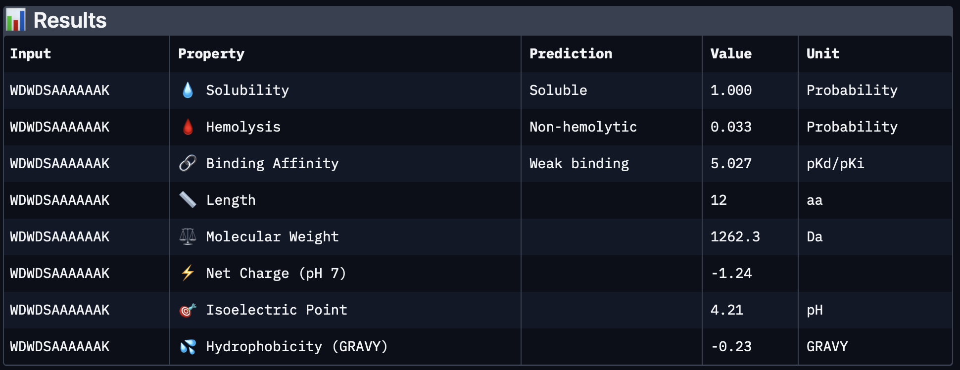
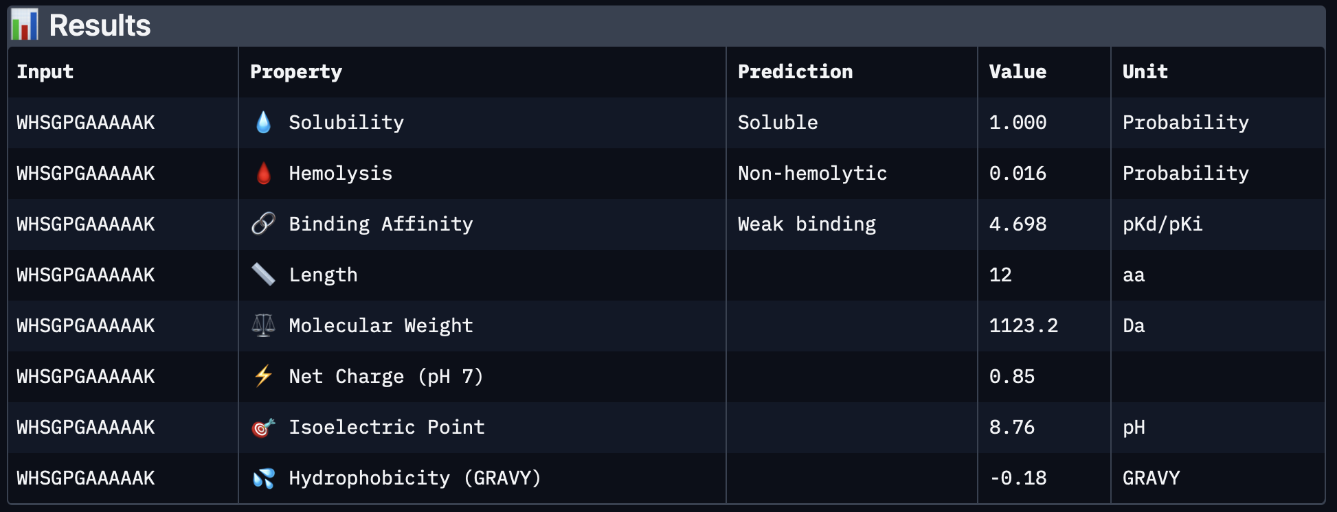
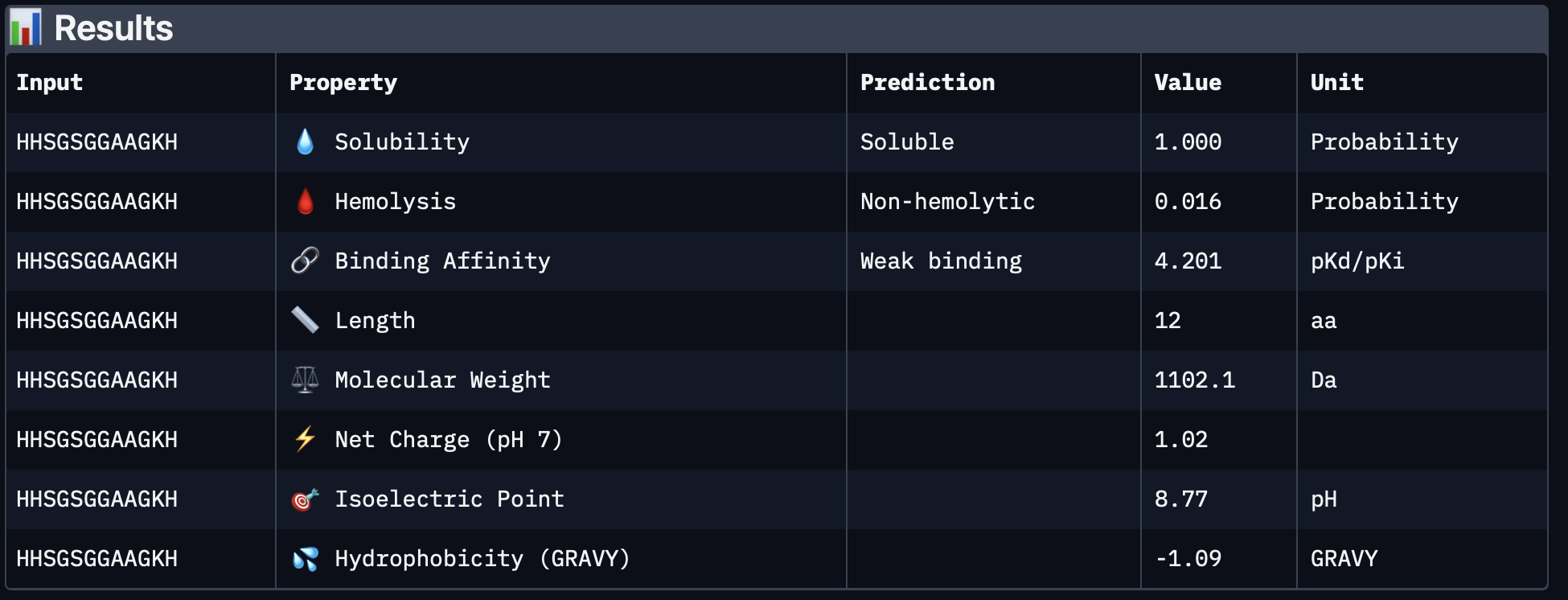
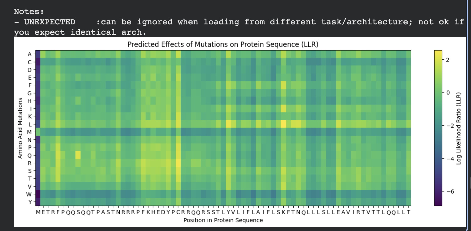
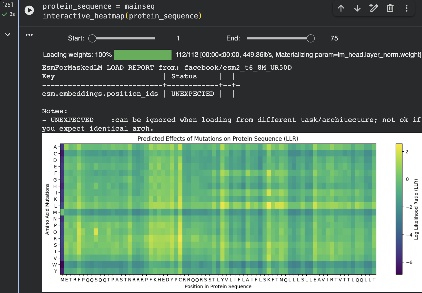
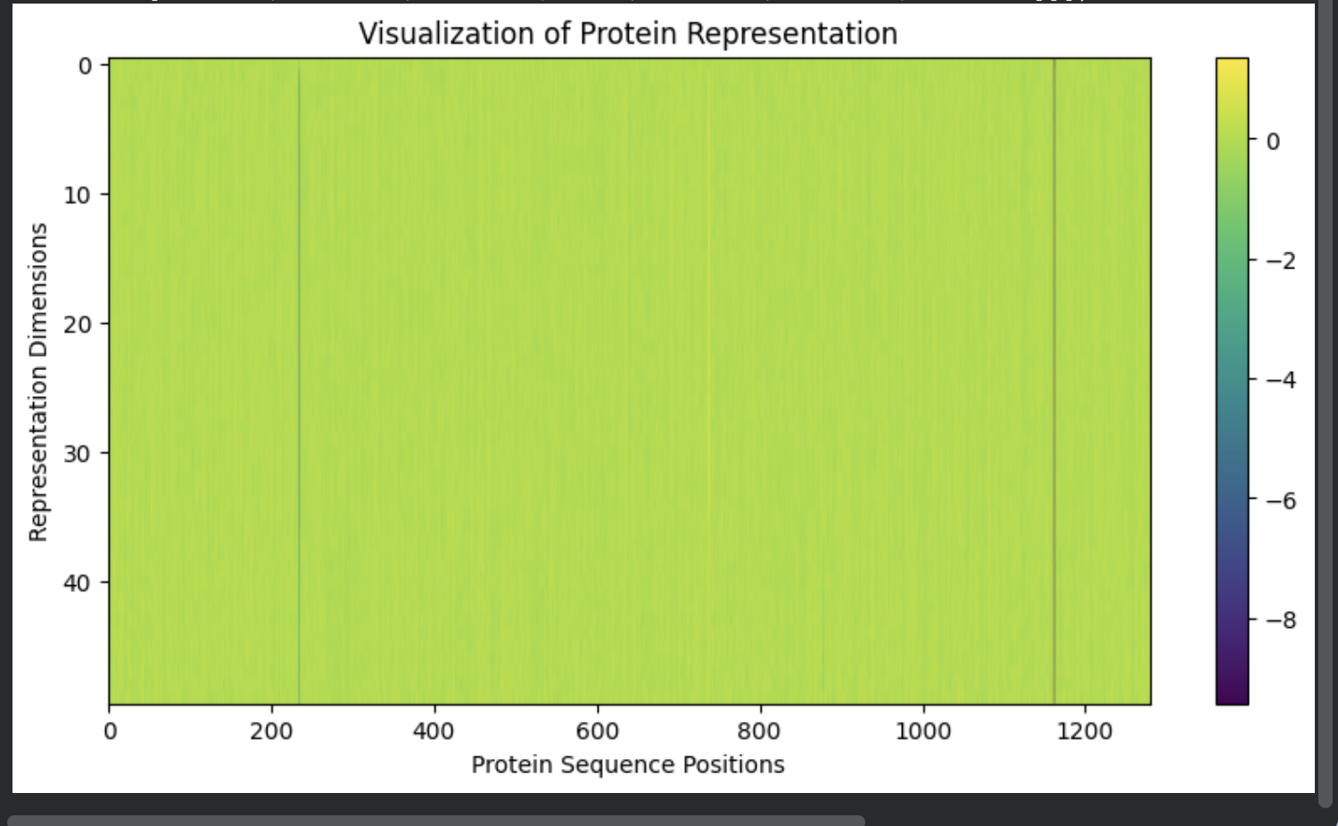
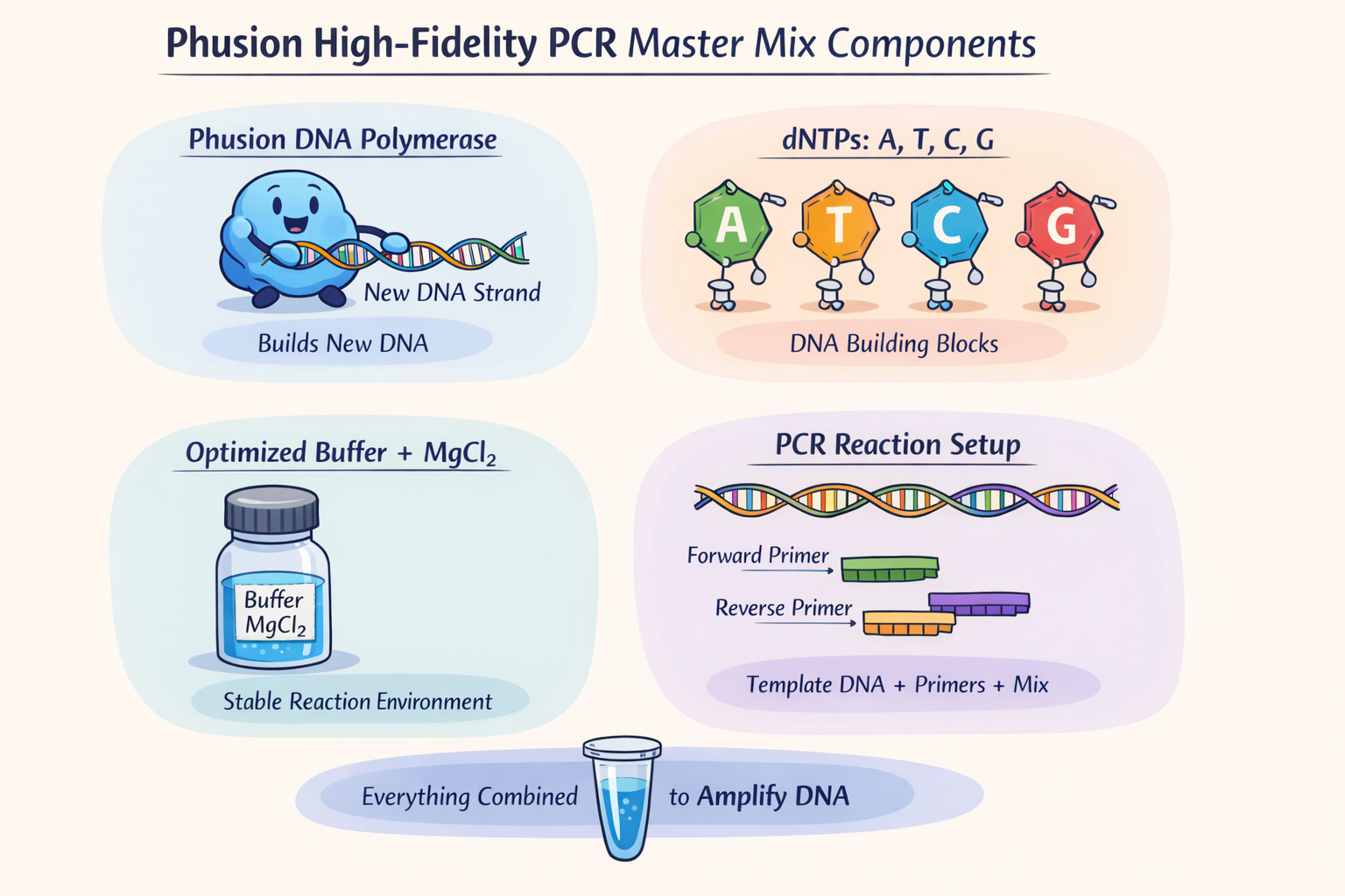
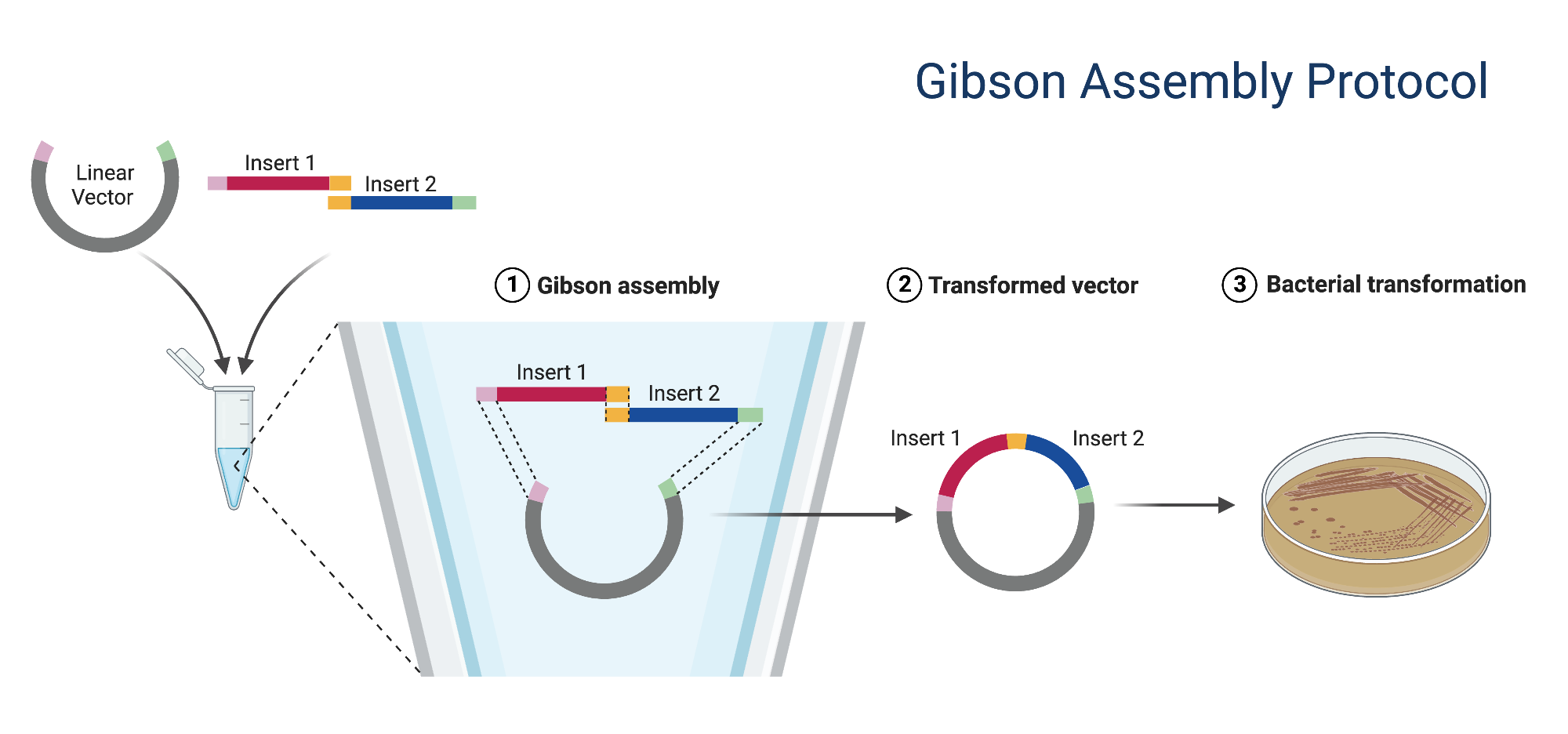
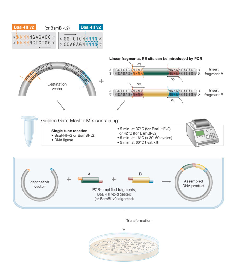
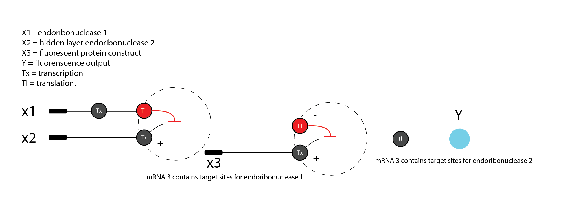
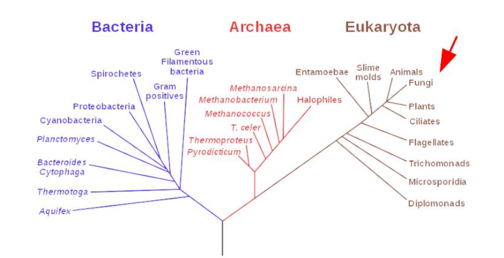
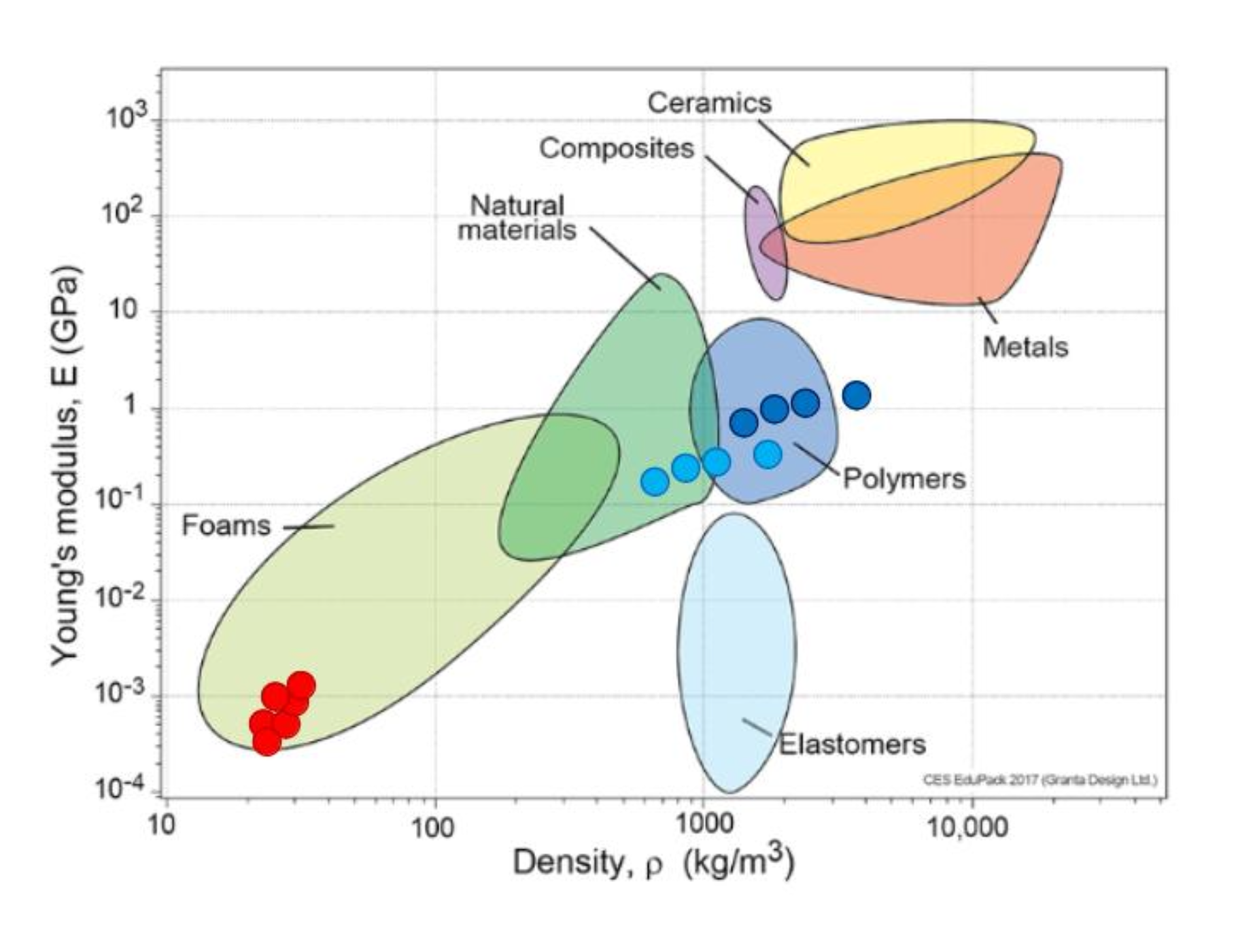
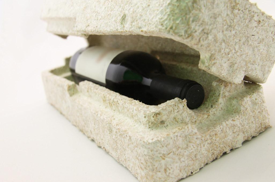
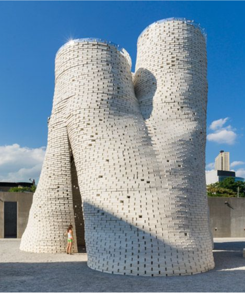
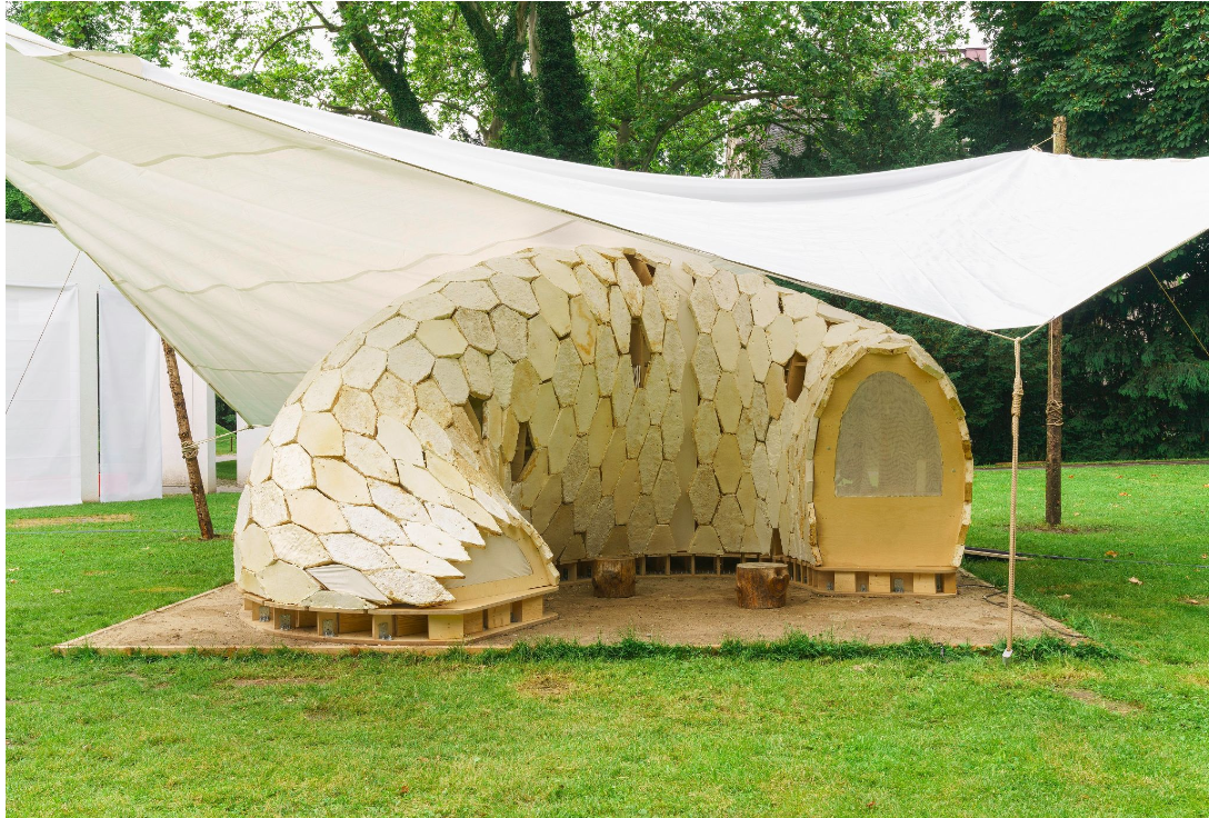
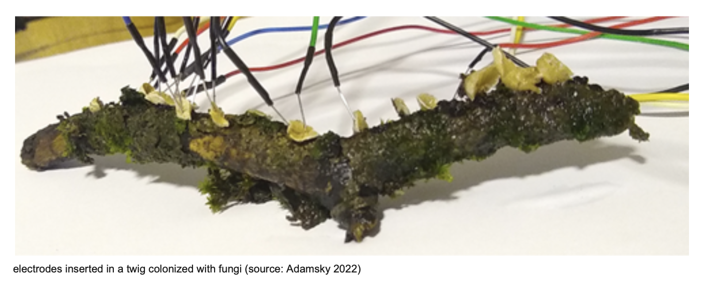
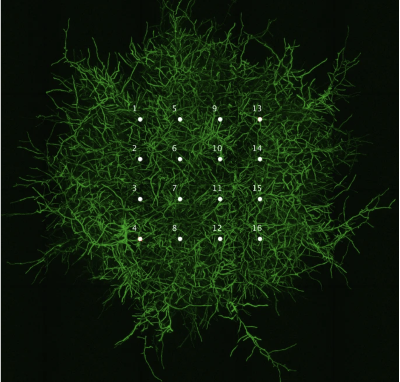
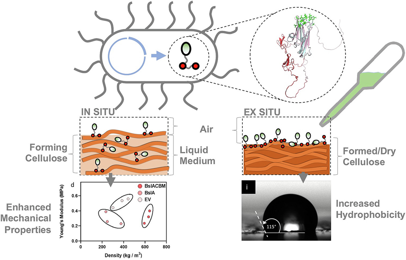
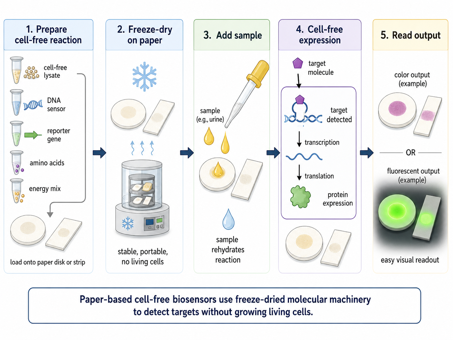
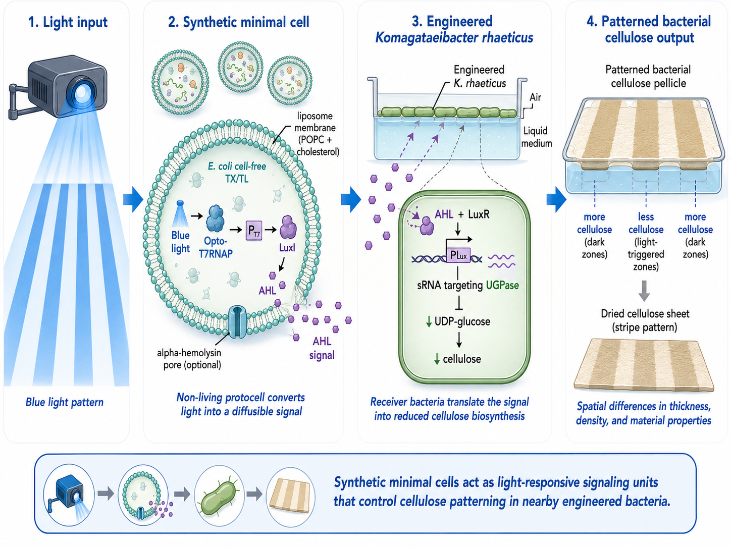
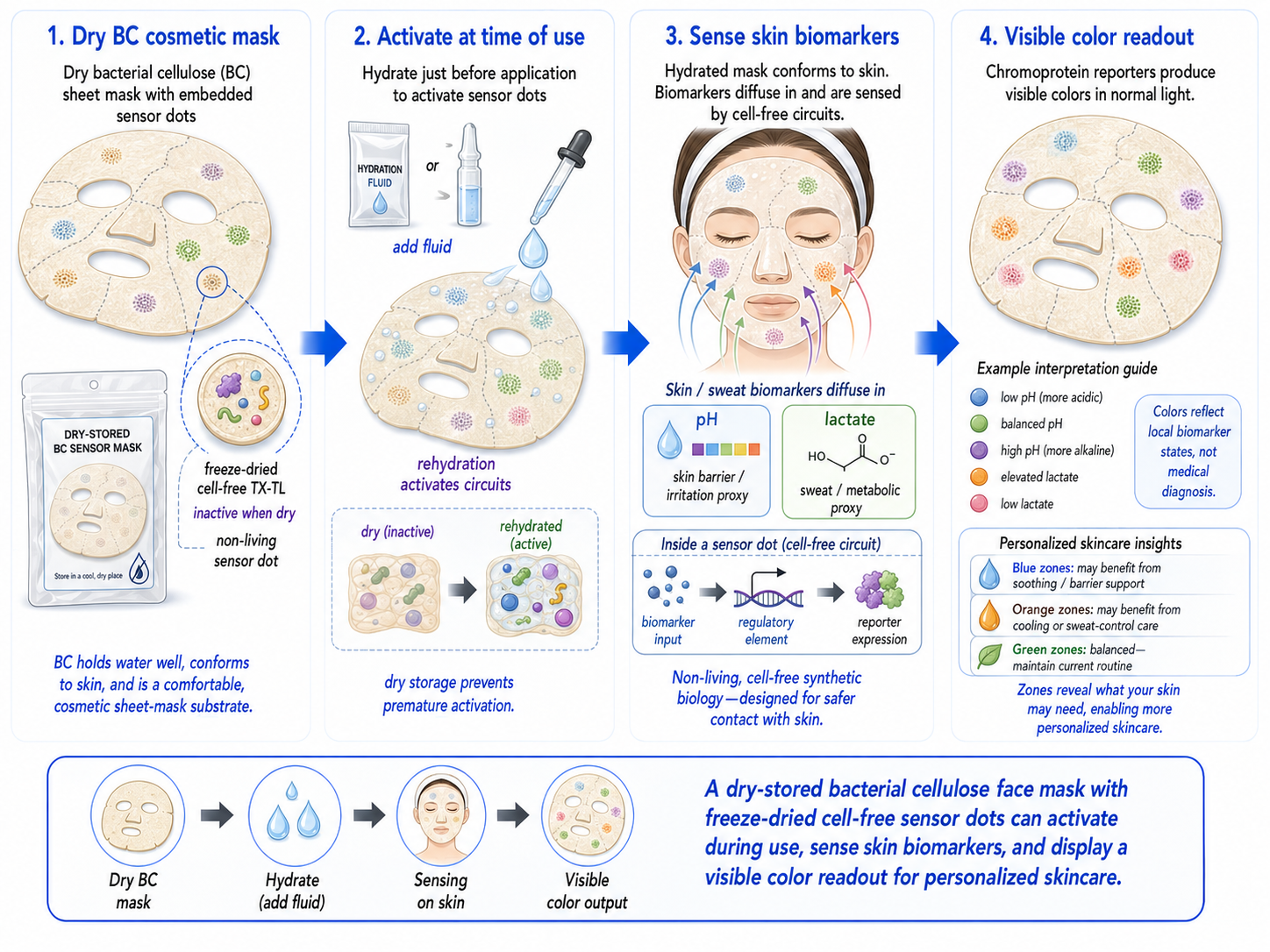
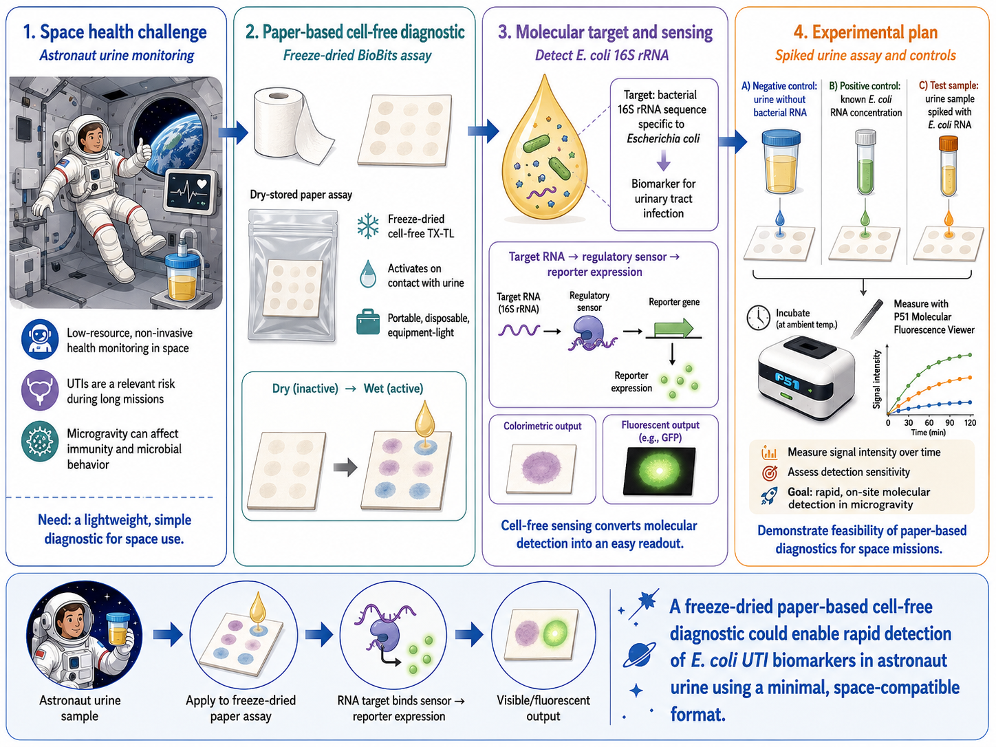
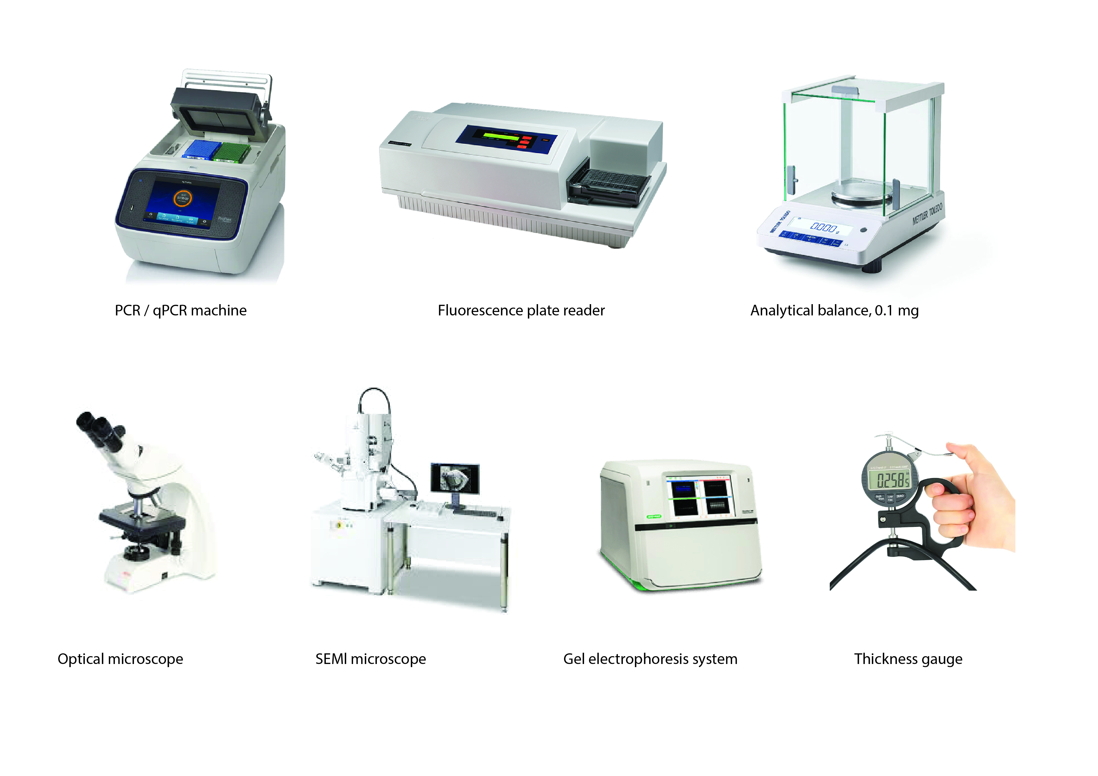
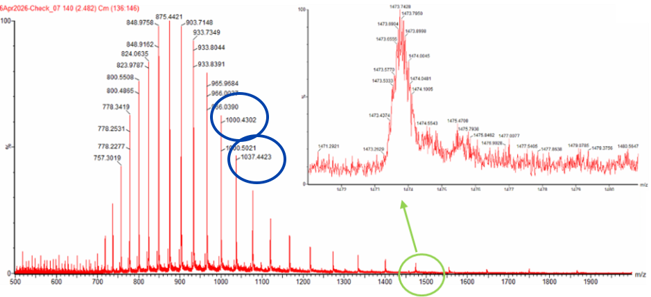
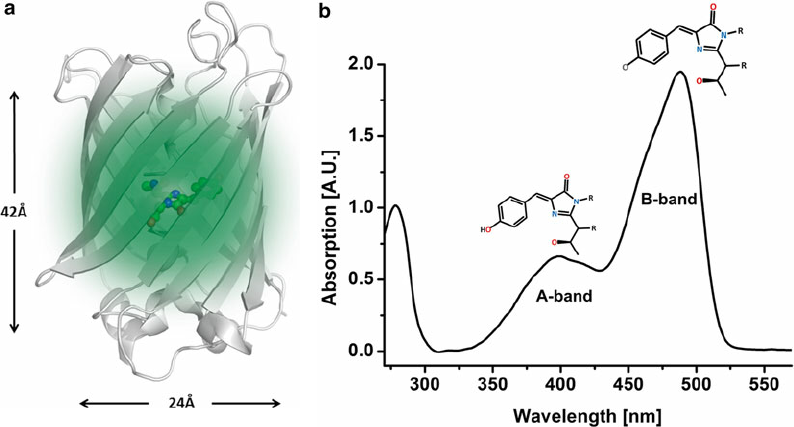
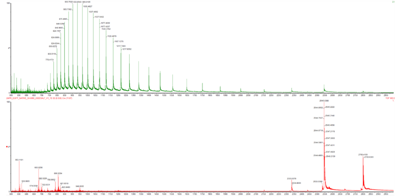
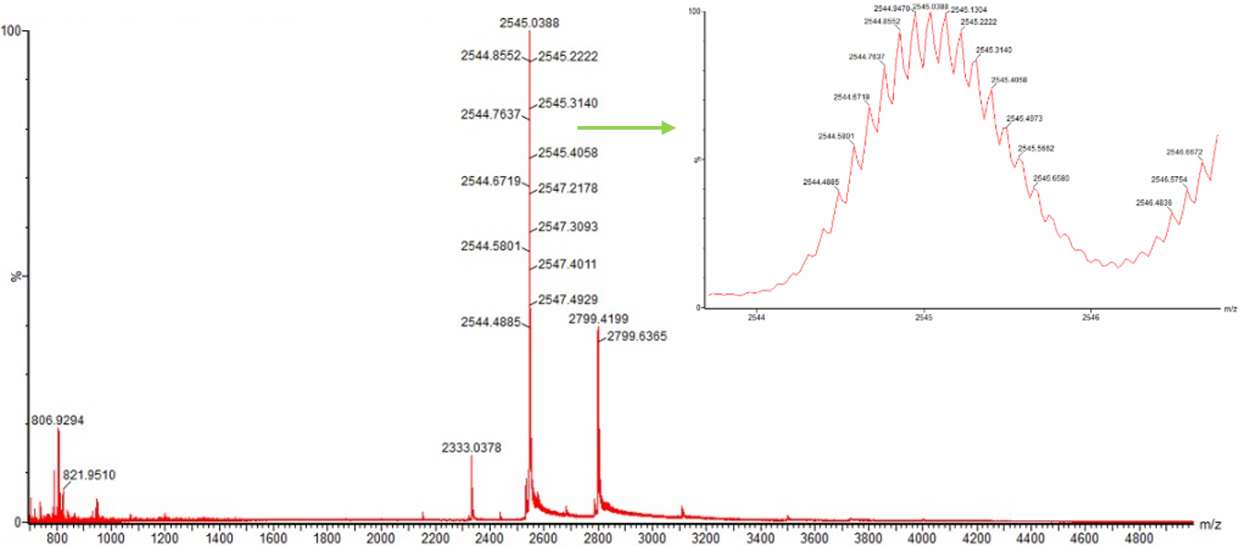
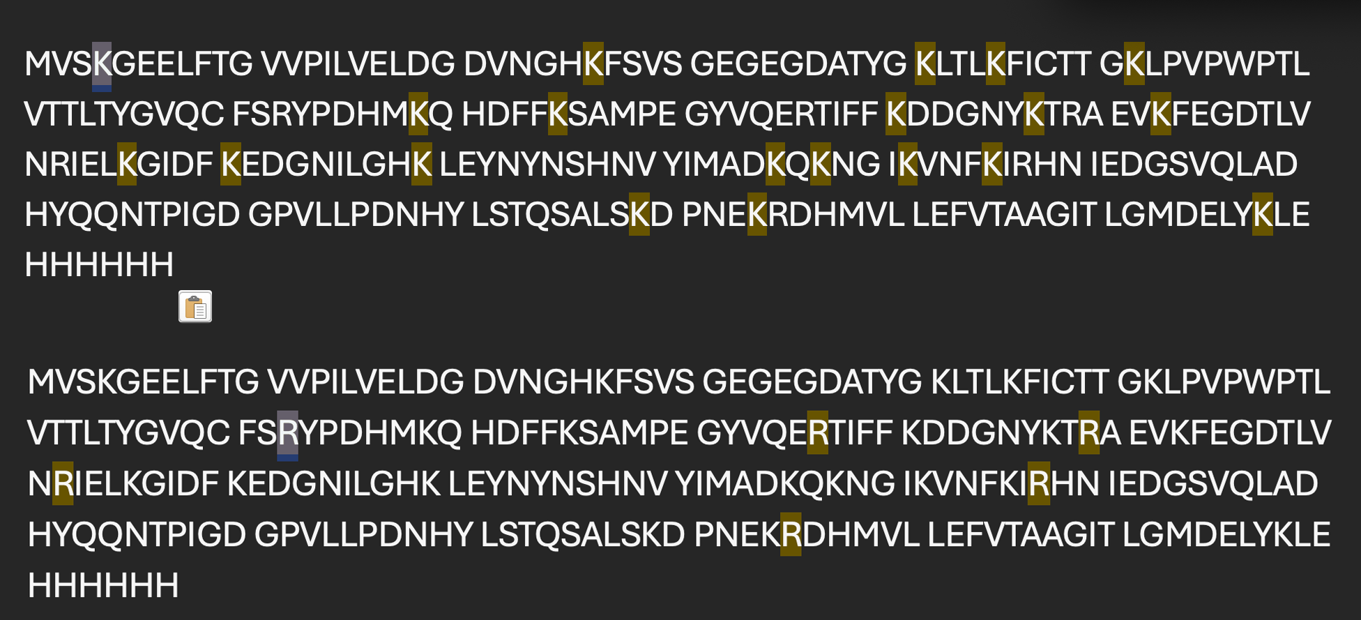
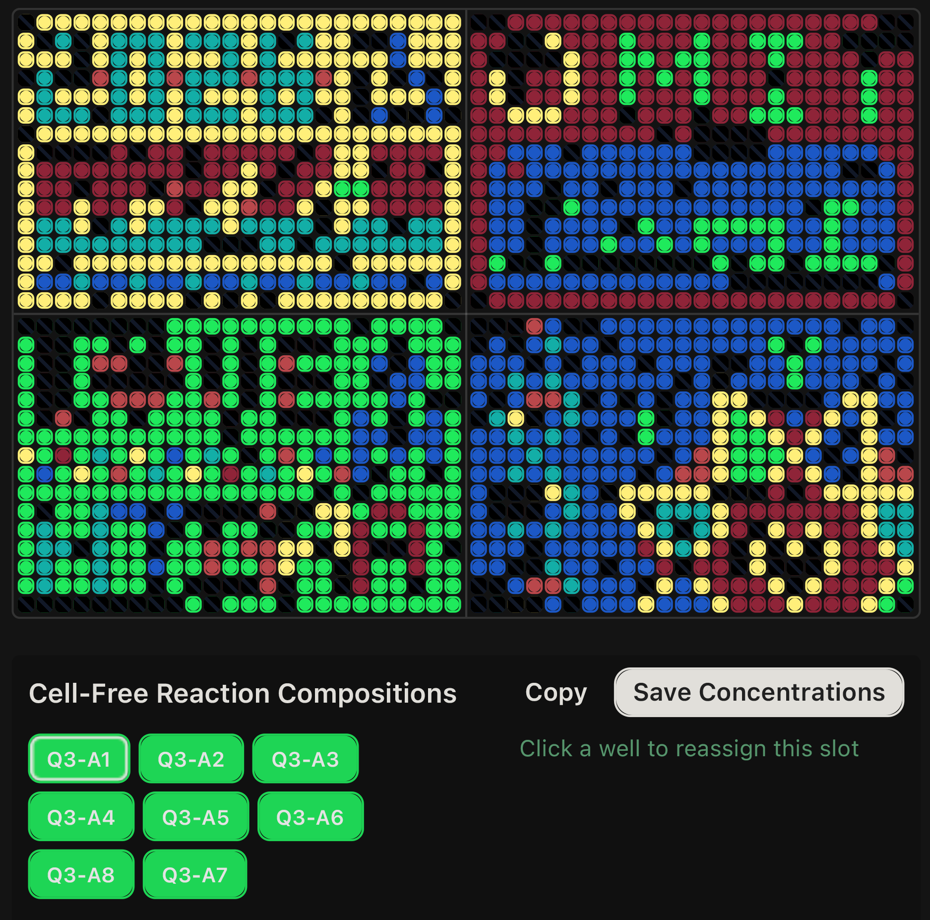
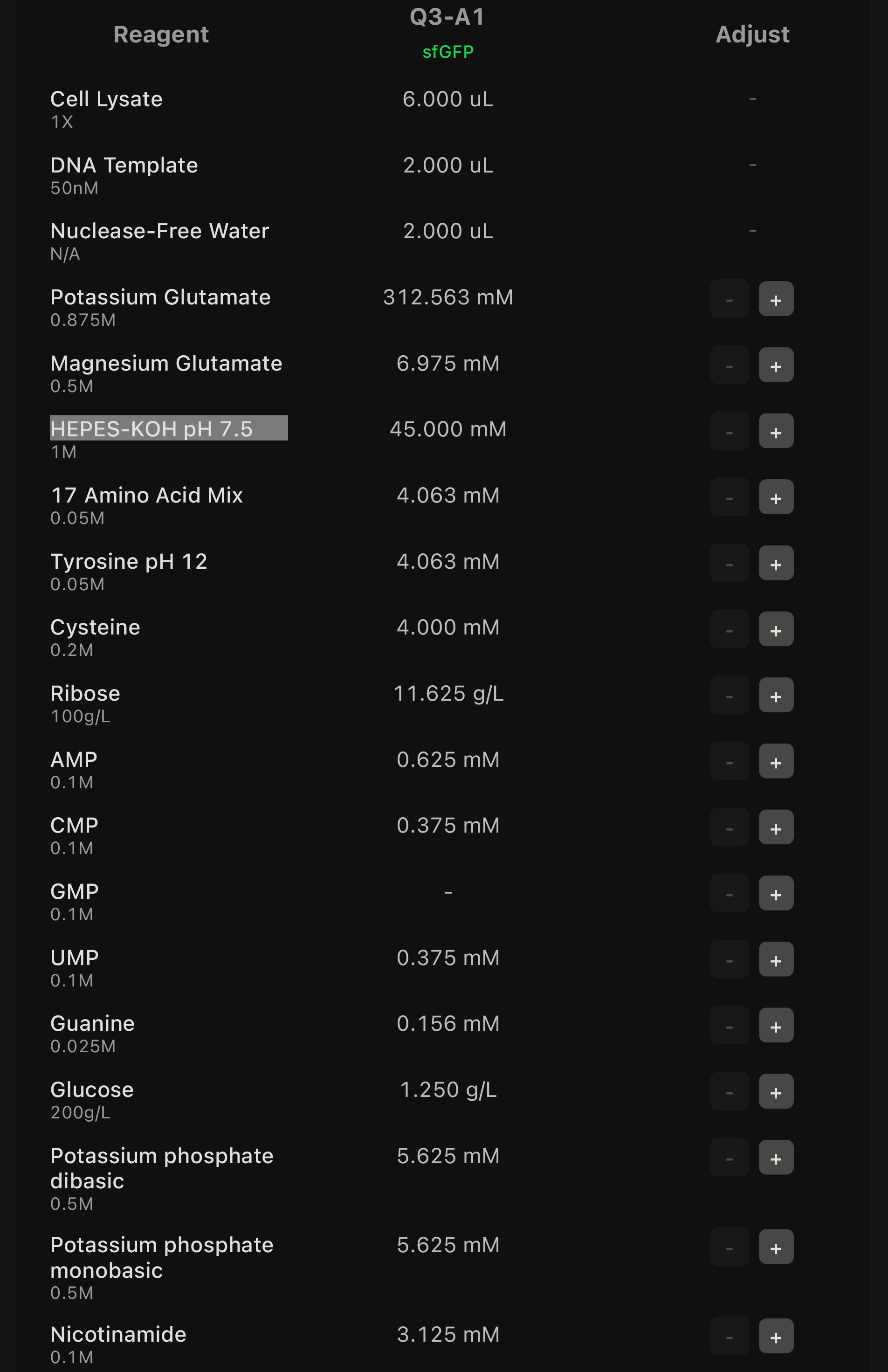