Week 04 HW: Protein design part 1
Shuguang Zhang — 9 Short Answers
(Skipped #4 and #11)
1. How many amino acid molecules are in 500 g of meat?
If 500 g of meat is about 20% protein, that gives about 100 g protein.
Since one amino acid is about 100 g/mol, that is about 1 mole, or ~6 × 10^23 molecules.
2. Why do we eat beef but do not become a cow?
Because our body digests food proteins into amino acids and then uses them to build human proteins.
3. Why are there only 20 natural amino acids?
Because evolution selected a set of 20 that gives enough chemical variety while still being efficient for life to use.
5. Where did amino acids come from before life started?
They likely formed through prebiotic chemistry, such as lightning, UV radiation, hydrothermal activity, or from meteorites.
6. What handedness would an α-helix made of D-amino acids have?
It would most likely form a left-handed helix.
7. Can there be additional helices in proteins?
Yes. Besides the α-helix, proteins can also have 3₁₀ helices and π-helices, and new ones can be designed.
8. Why are most molecular helices right-handed?
Because natural proteins are made from L-amino acids, which usually favor right-handed helices.
9. Why do β-sheets tend to aggregate?
Because β-strands can easily line up and make hydrogen bonds with each other.
The main driving force is backbone hydrogen bonding plus hydrophobic interactions.
10. Why do many amyloid diseases form β-sheets? Can amyloid β-sheets be used as materials?
Amyloid proteins often misfold into very stable β-sheet fibrils, which can build up in disease.
Yes, in controlled settings they can also be used as useful biomaterials.
Before diving deep into the homework here is some highlight from the lecture with Cale and Ahmed giving some fundational knowledge around protein design:
what does protein do?

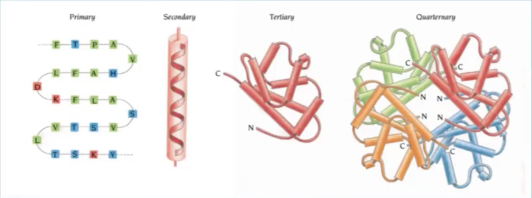
When we look at protein design it is important to concider what type of abstraction we are looking at:
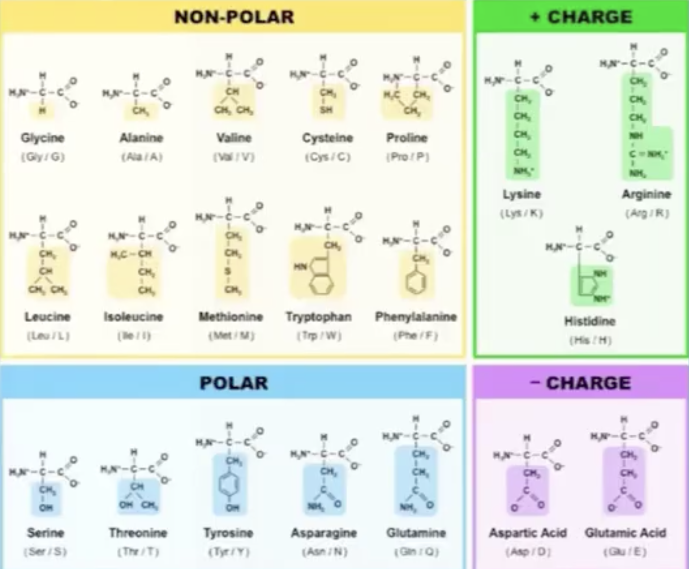
Proteins are build up from the 20 Amino acids each has a unique chemical structure, charge, physical propertie that will determine the protein structure and function:
this is an overview of the most important function of proteins:
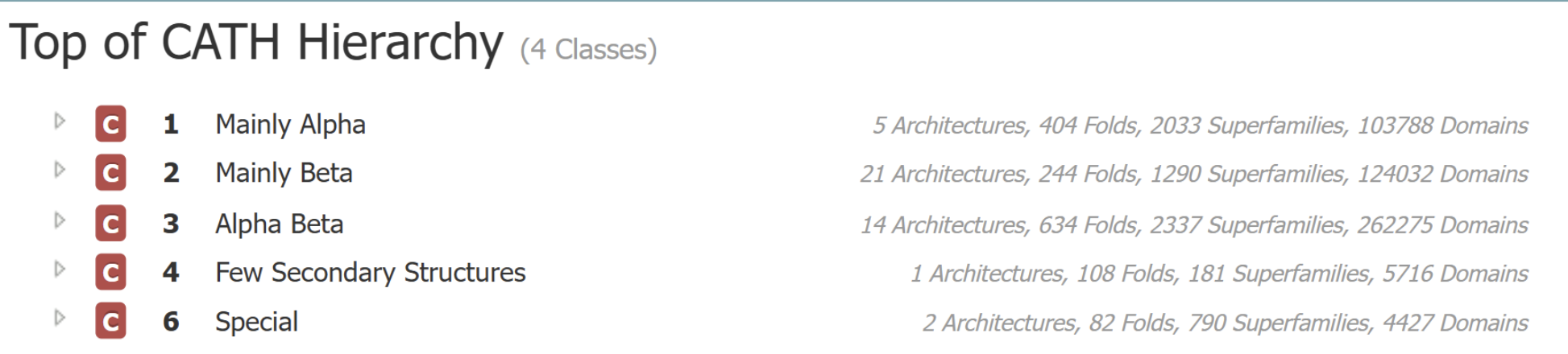
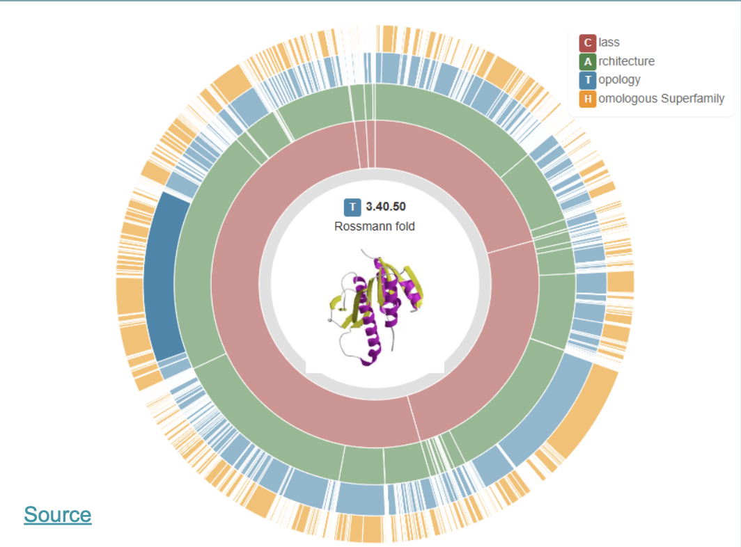
Proteins are classified as CATH
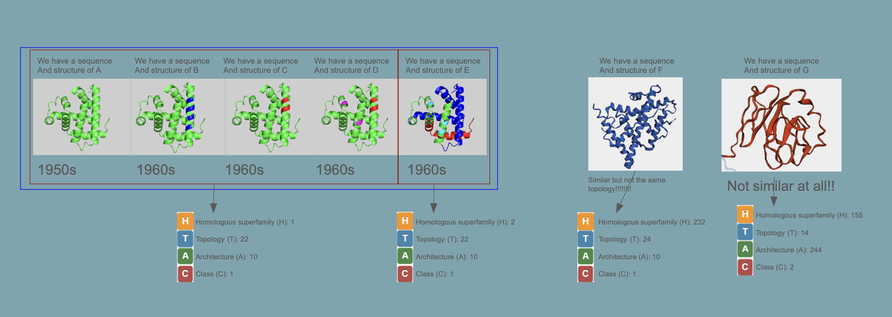
This is a great website where you easily can “browse” the different classes:
Distance maps are a tecnique to calculate distance between different parts in space of a protein structure and visualize it in 2D (scale: ångstrom)

Three scoring categories of the quality of predicted structure:
- Physical / Energetic
- Stability, folding energy,
- Examples: Rosetta energy, ΔG folding
- Structural
- RMSD, Packing, clashes
- Models confidence
- AlphaFold pLDDT / PAE
plddt usage:
- Assessing confidence within a domain ((but not between domains))
- Identifying domains
- Identifying possible disordered regions
PAE usage:
- To assess relative domain positions
- If the value is less than 30 in the interface region means a good predictor of binding
Part B — Protein Analysis and Visualization (BcsZ / PDB: 3QXF)
Table of contents
- 1. Protein choice
- 2. Amino acid sequence + basic analysis
- 3. Homologs (UniProt BLAST)
- 4. Protein family / domain classification
- 5. Structure page + structure quality
- 6. Structure classification (SCOP2 / CATH / ECOD)
- 7. 3D visualization in PyMOL
- Appendix: code + commands
1. Protein choice
I chose BcsZ (bacterial cellulose synthase subunit Z) from Escherichia coli K-12 (PDB: 3QXF) because it is part of the bacterial cellulose (BC) synthase system. BcsZ is annotated as a periplasmic endo-β-1,4-glucanase in glycoside hydrolase family 8 (GH8), meaning it can cut β-1,4 linked glucan chains (cellulose-like polymers) and is associated with efficient cellulose biosynthesis/translocation.
What “periplasmic endo-β-1,4-glucanase (GH8)” means
- Periplasmic: located in the periplasm, the space between inner and outer membranes in Gram-negative bacteria (like E. coli).
- Glucan: a chain of glucose units (cellulose is a glucan).
- β-1,4: the bond type between glucose units in cellulose.
- Endo-: cuts inside the chain (not only from the ends).
- GH8: a carbohydrate-enzyme family classification (shared fold + mechanism among related enzymes).
Why a cellulose-producing bacterium has a “cellulose cutter” Producing and exporting a long polymer is mechanically challenging. A periplasmic endoglucanase can help by:
- clearing jams / trimming chains that clog export
- processing cellulose during extrusion (helps proper fiber/network formation)
- helping polymer movement through the periplasm toward the export channel
2. Amino acid sequence + basic analysis
Sequence source: RCSB PDB sequence for 3QXF, chain A www.rcsb.org.
Sequence length: 355 aa (chains A–D are the same sequence).
FASTA (chain A)
Amino-acid frequency (from the Week 4 Colab)
I used the Week 4 Colab notebook to compute amino-acid frequencies from the FASTA sequence.
Most frequent amino acids (top 5):
- A (Alanine): 32
- L (Leucine): 31
- G (Glycine): 26
- S (Serine): 23
- K (Lysine): 22 (tied with D = 22)
I used ChatGBT to generate this code that could generate most frequent AA:
3. Homologs (UniProt BLAST)
I ran UniProt BLAST (https://www.uniprot.org/blast) using the FASTA sequence above (default settings).
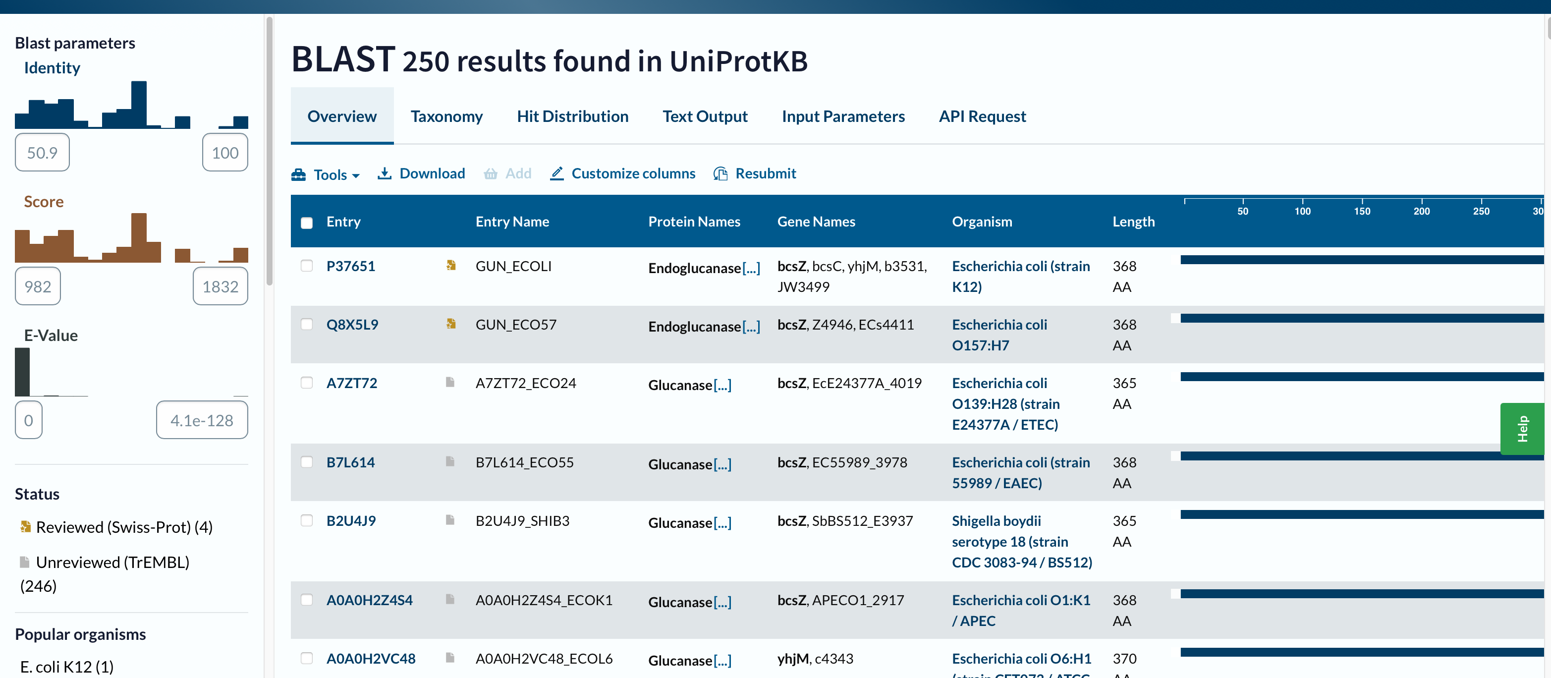
- Homologs found (displayed): 250 results in UniProtKB
- E-value range shown: from 0.0 (strongest) to about 4.1 × 10⁻¹²⁸ (least significant shown)
- Identity range shown: approximately 50.9% – 100%
- Example top hit (from Text Output): 99% identity (338/339), Expect = 0.0
Conclusion: With the displayed results, all 250 hits are >30% identity, and all are extremely significant by E-value.
Footnote:
- Homologs are proteins in other organisms (or strains) that are related by evolution—they come from a common ancestral gene.
- The E-value (expect value) is a BLAST statistic that answers: “If I searched a database this big with a random (unrelated) sequence, how many hits with this score would I expect to see just by chance?”
- Rule-of-thumb:
- E < 1e-3: usually meaningful similarity
- E < 1e-10: very strong
- E ~ 0.0 (BLAST rounds extremely tiny values to 0): essentially “as strong as it gets”
4. Protein family / domain classification
Does it belong to a protein family? Yes.
But first of all what is CATH, SCOP2 and ECOD:
CATH, SCOP2, and ECOD are all systems for classifying protein domains based on their three-dimensional structure and evolutionary relationships, but they organize proteins in slightly different ways. CATH uses a clear hierarchical scheme based on Class, Architecture, Topology, and Homologous superfamily, making it useful for describing both structural shape and evolutionary grouping. SCOP2 is an updated version of SCOP that also classifies proteins by structure and ancestry, but it uses a more flexible framework rather than a strictly rigid hierarchy. ECOD (Evolutionary Classification of Protein Domains) places particularly strong emphasis on evolutionary relationships and homology, aiming to group protein domains by shared ancestry. In summary, all three classify protein structure, but CATH is often seen as a geometry-based hierarchical system, SCOP2 as a flexible structure-and-evolution system, and ECOD as especially focused on evolutionary history.
- GH8 (Glycoside Hydrolase family 8): indicates BcsZ belongs to a known family of carbohydrate-active enzymes that hydrolyze glycosidic bonds (fits its endoglucanase/cellulase-like role).
- Six-hairpin glycosidase(-like) superfamily: describes the shared fold architecture (a helix-rich α/α toroid / alpha–alpha barrel-like fold) found in related carbohydrate enzymes, even when sequences vary.
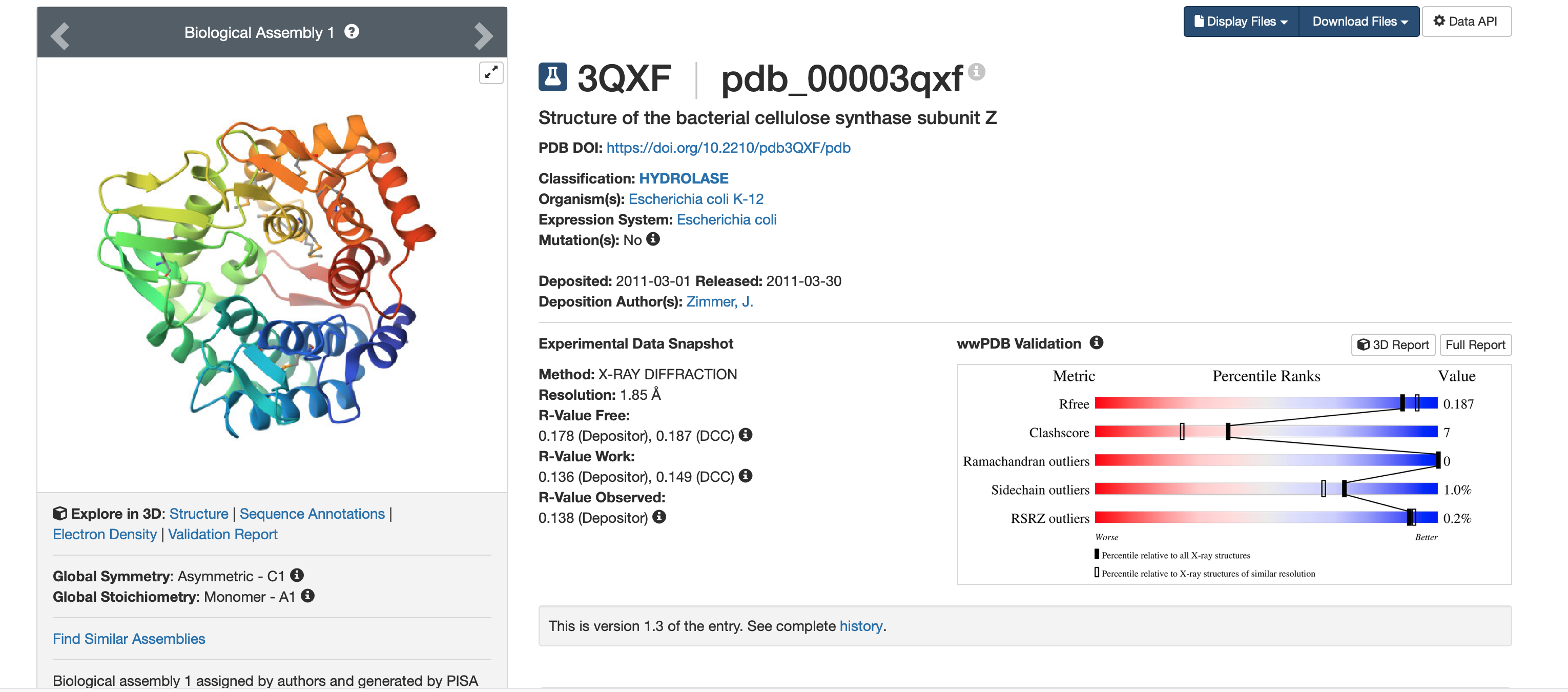
5. Structure page + structure quality
From the RCSB structure page www.rcsb.org:
- PDB entry: 3QXF
- Method: X-ray diffraction
- Resolution: 1.85 Å (high quality; smaller Å = sharper structure)
- Released: 2011-03-30 (deposited 2011-03-01)
- Other molecules present: Other molecules present: no ligands/cofactors (HET atoms = 0), but the crystal includes waters (solvent); the protein was expressed with selenomethionine (MSE) residues.
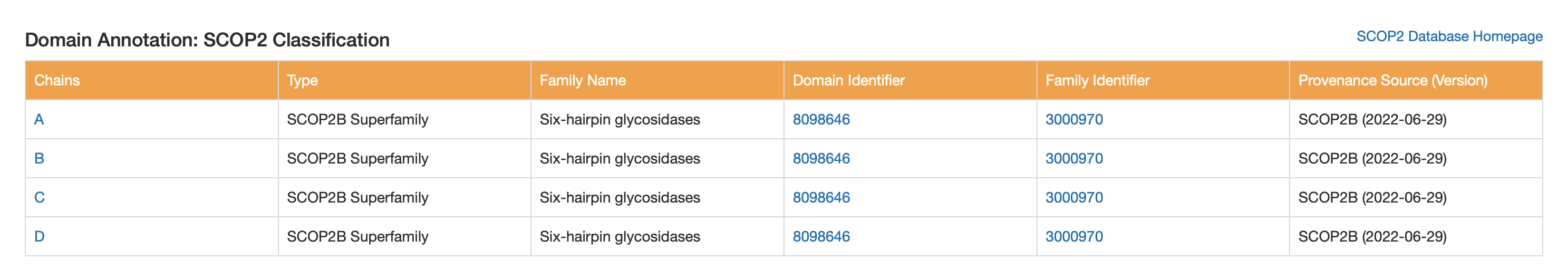
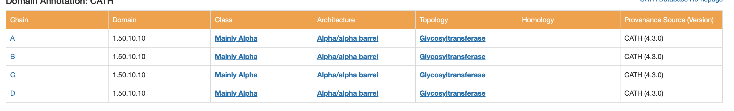
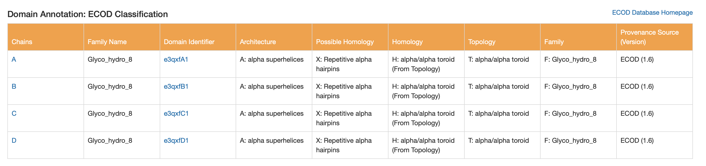
6. Structure classification (SCOP2 / CATH / ECOD)
These classifications all point to a helix-rich α/α architecture typical of GH8-like glycosidases.
SCOP2
- SCOP2B Superfamily: Six-hairpin glycosidases
CATH
- Class: Mainly Alpha
- Architecture: Alpha/alpha barrel
ECOD
- Architecture: alpha superhelices
- Topology: alpha/alpha toroid
- Family name: Glyco_hydro_8
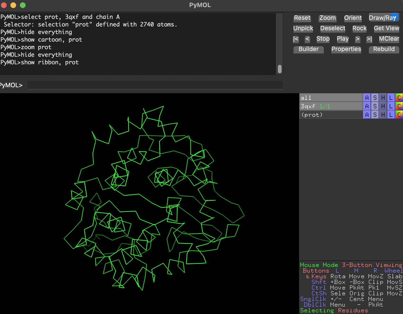
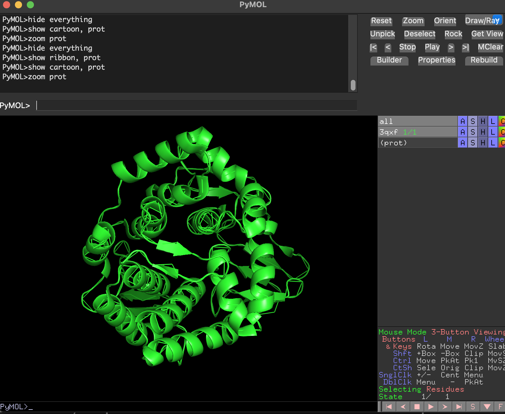
7. 3D visualization in PyMOL
I used PyMOL to visualize 3QXF (focusing on chain A for clarity).
7.1 Visualize as cartoon, ribbon, and ball-and-stick
- Ribbon
- Cartoon
- Ball-and-stick Full-protein ball-and-stick is visually dense but shows atomic detail.
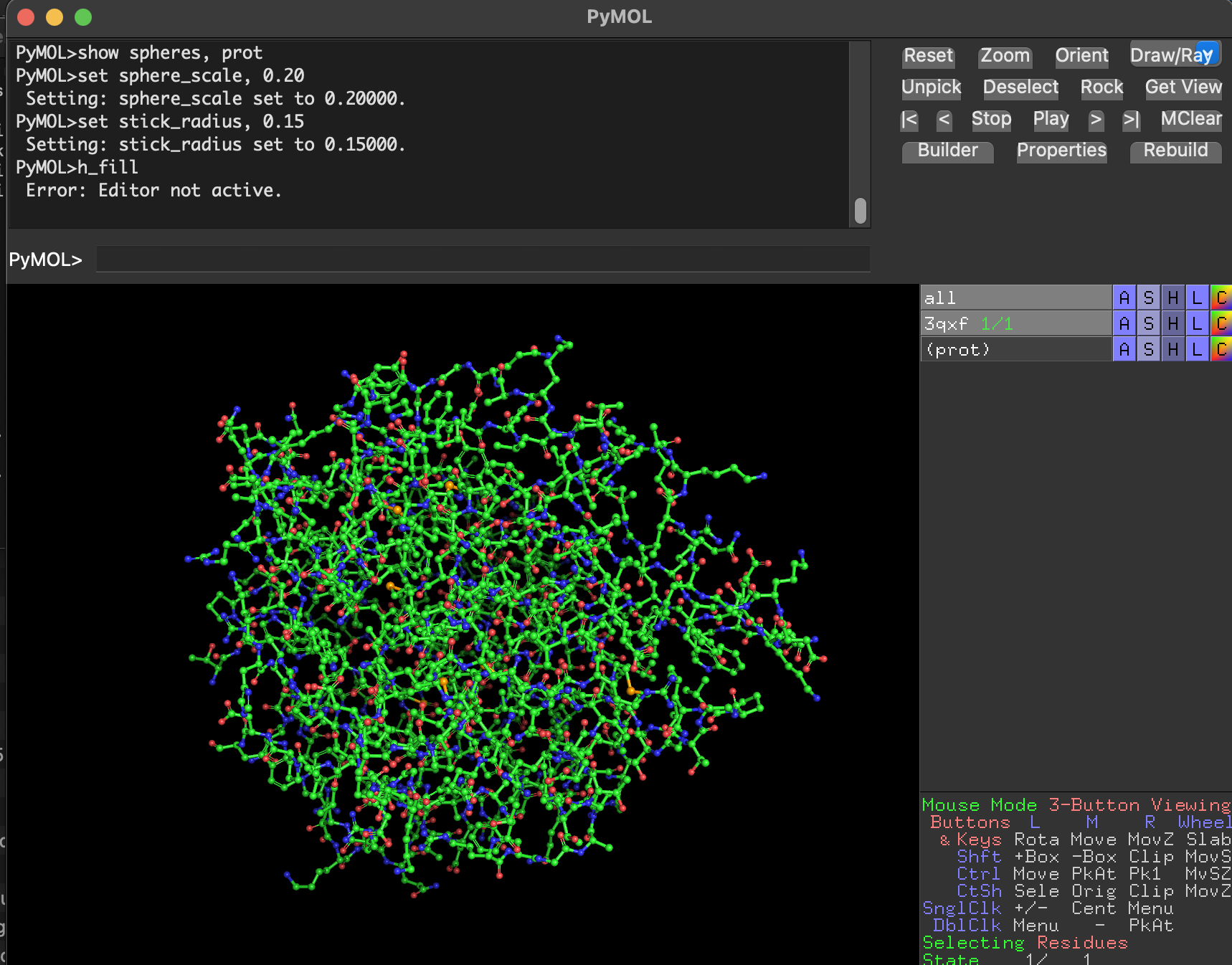
Why are we using this 3 ways of visualize the protein structure?
- Cartoon/ribbon answer: What is the big structural arrangement?
- Ball-and-stick answers: What is happening at the residue/atom level?
7.2 Color by secondary structure. Does it have more helices or sheets?
After coloring by secondary structure:
- Helices dominate (in red)
- There are fewer β-sheets (in yellow)
- Remaining regions are loops/turns
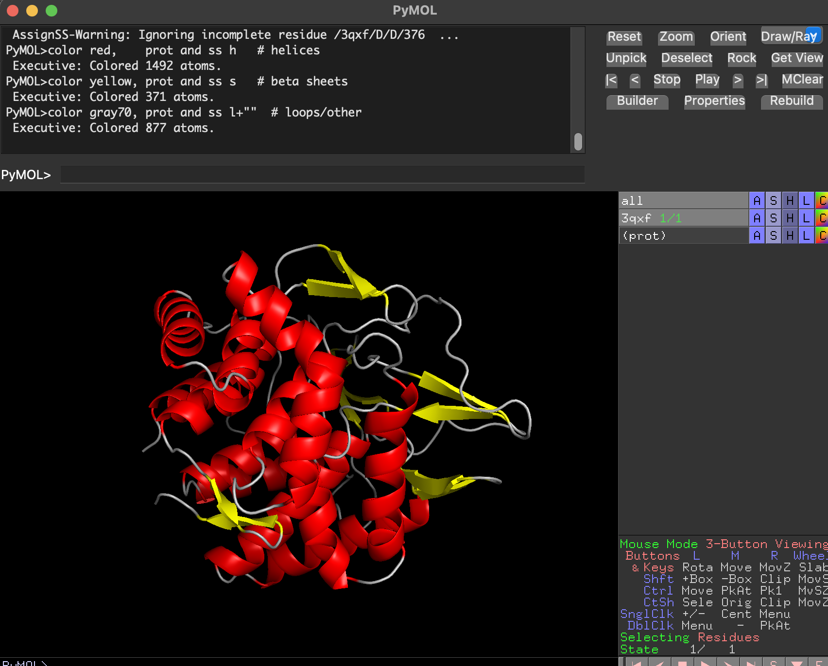
Conclusion: BcsZ is helix-rich (more helices than β-sheets), consistent with GH8 / α/α fold classifications.
7.3 Color by residue type. Hydrophobic vs hydrophilic distribution
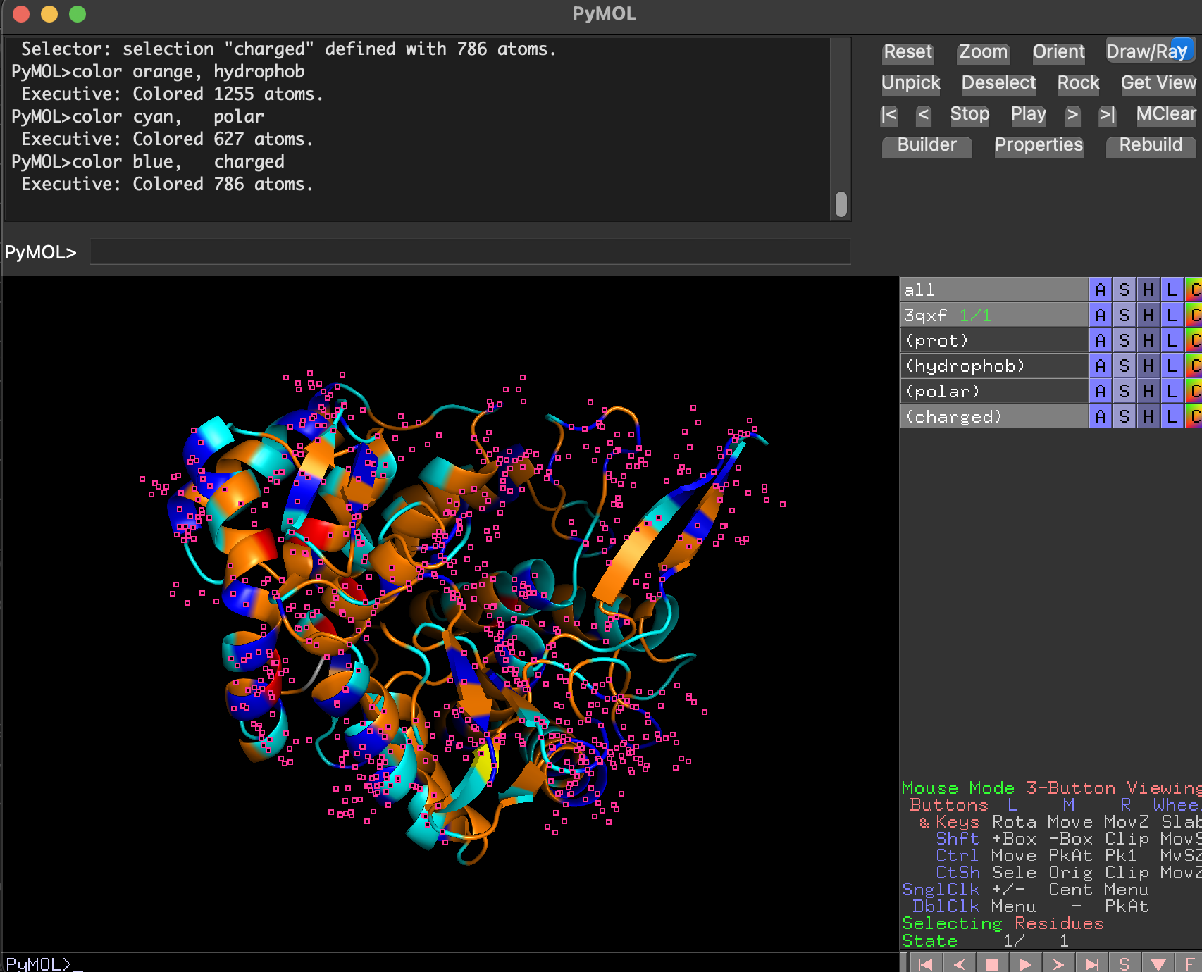
After coloring residues by type:
- Hydrophobic residues (orang) cluster mostly in the protein core (stabilizing the fold).
- Polar and charged residues (cyan) are enriched on the protein surface, consistent with a soluble enzyme.
- charged is colored in blue
- The putative substrate-binding cleft shows a mix of polar/aromatic residues typical for carbohydrate-binding enzymes.
Note The small pink dots are likely selenium-containing atoms from selenomethionine (MSE) residues present in the crystal structure. Since MSE was not included in the custom residue-type selections, those atoms remained in the default viewer coloring.
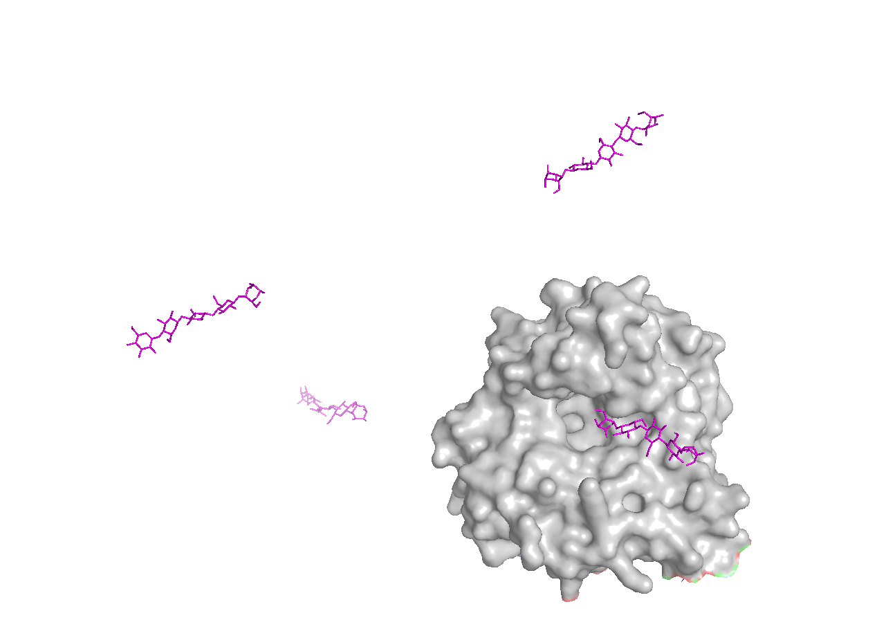
7.4 Visualize the surface. Does it have any “holes” (binding pockets)?
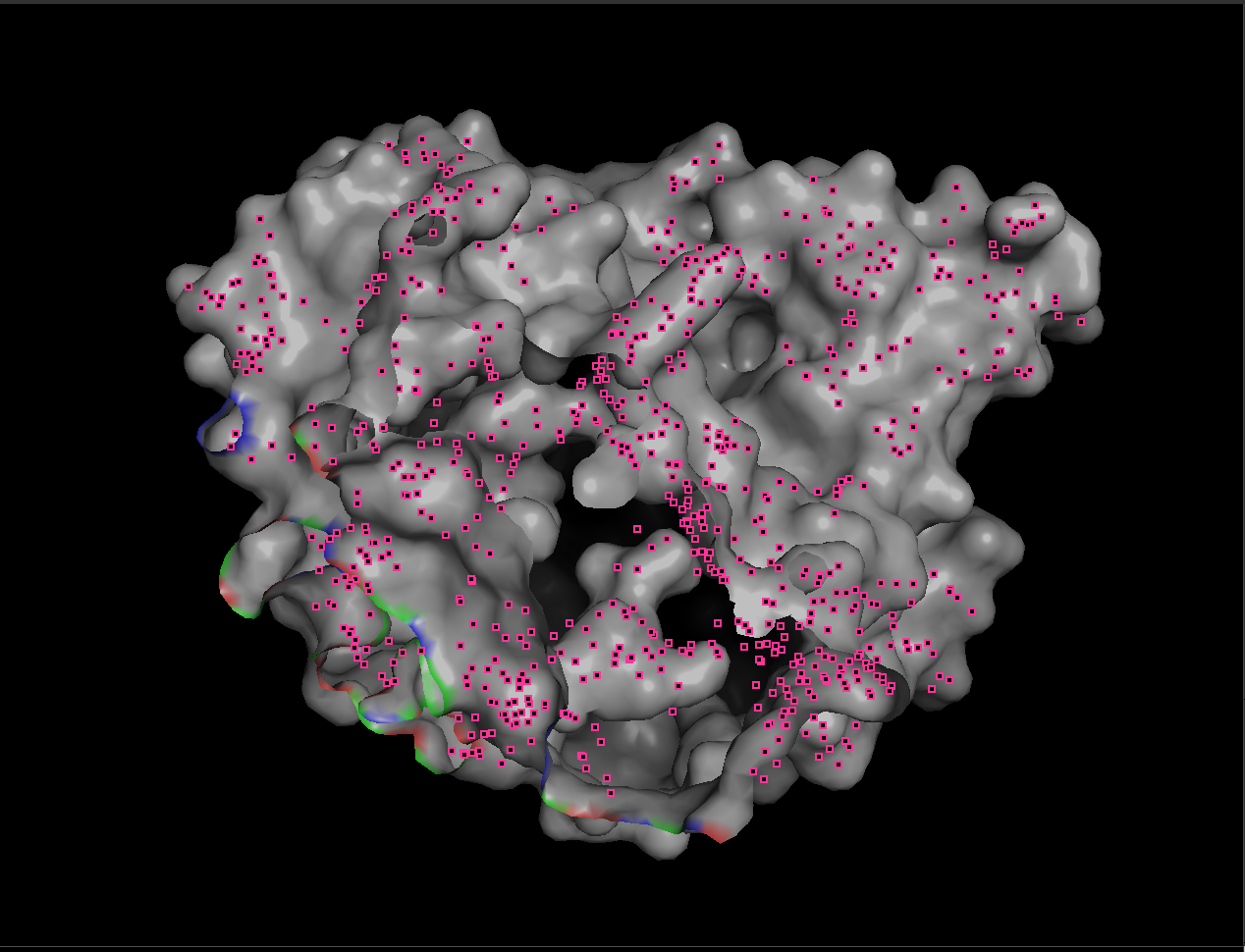
When visualized as a surface, BcsZ shows a prominent groove/cleft rather than a deep enclosed cavity.
Conclusion: BcsZ has a clear binding pocket / cleft consistent with an enzyme that acts on polymeric substrates (cellulose-like chains), which often bind along an open channel rather than a small closed pocket.
- A small closed pocket is good for binding a small molecule.
- An open groove or cleft is better for binding a long chain, like cellulose.
To make the substrate-binding cleft clearer, I compared the apo BcsZ structure (3QXF) with the cellopentaose-bound BcsZ structure (3QXQ), which shows how a glucan chain can sit along the open cleft.
C1. Protein Language Modeling — Unsupervised Deep Mutational Scan (ESM2)
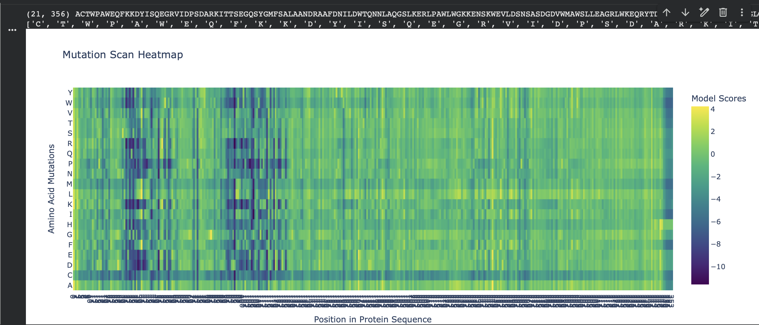
For my chosen protein (PDB: 3QXF), I used ESM2 to generate an unsupervised deep mutational scan by scoring every possible single amino-acid substitution at each position (language-model likelihood scores, mode="RELATIVE"). In the heatmap, each column is a residue position in the sequence and each row is a mutation-to amino acid. Brighter colors indicate mutations the model considers more plausible in context; darker colors indicate mutations that are strongly disfavored.
Overall pattern (what the heatmap shows)
Most positions show modest tolerance (many mutations cluster around neutral-ish scores), but there are clear vertical bands of strongly negative scores where almost any substitution is unlikely. These “dark stripes” suggest highly constrained positions, often linked to structural packing or important local geometry.
Finding standout mutations (min/max scores)
Because N- and C-termini can show edge effects in language-model scoring (and my sequence ends with a short His-tag tail), I selected a standout mutation after excluding:
- the first 5 residues (N-terminus edge effects)
- the last 7 residues (His-tag tail)
I used the code below to convert the heatmap matrix into a mutation table and extract the most damaging/tolerated substitutions:
Standout example (a strongly constrained position)
Most damaging internal mutation: V98 → R, score −11.600975
This mutation replaces a small hydrophobic residue (Val) with a bulky, positively charged residue (Arg). That kind of change is typically unfavorable if the position is in a packed protein interior (it disrupts hydrophobic packing and can introduce an unsatisfied charge). The fact that multiple substitutions at the same site are also strongly negative suggests position 98 is broadly mutation-intolerant, consistent with it being structurally important.
Top 10 most damaging (excluding first 5 residues + His-tag tail)
| Rank | Position | WT → Mut | Score |
|---|---|---|---|
| 1 | 98 | V → R | -11.600975 |
| 2 | 109 | R → I | -11.381086 |
| 3 | 107 | A → P | -10.845333 |
| 4 | 41 | F → D | -10.764390 |
| 5 | 109 | R → L | -10.727297 |
| 6 | 41 | F → K | -10.649606 |
| 7 | 98 | V → C | -10.633169 |
| 8 | 98 | V → W | -10.569185 |
| 9 | 98 | V → K | -10.555022 |
| 10 | 102 | W → K | -10.527938 |
Extra pattern note: several top hits are “structurally disruptive” mutation types (e.g., A→P can break secondary structure; aromatic/hydrophobic → charged can disrupt packing or interfaces), which matches the intuition that the darkest vertical bands in the heatmap correspond to constrained, structure-critical sites.
C1. Protein Language Modeling — Latent Space Analysis (ESM2 embeddings + 3D t-SNE)
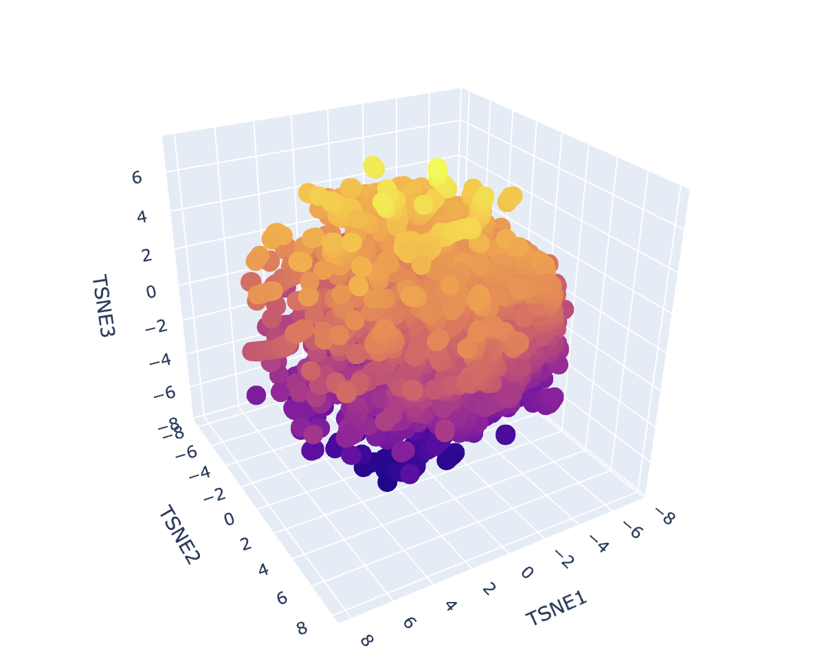
To explore how a protein language model organizes sequence space, I embedded a provided dataset of ~15k protein sequences using ESM2 and then reduced the embeddings to 3 dimensions with t-SNE. Each point in the plot corresponds to one protein from the dataset; proteins that are close together are similar in ESM2 embedding space (i.e., the model considers them “sequence-context similar”).
Note: t-SNE axes (TSNE1/TSNE2/TSNE3) are arbitrary visualization coordinates (they don’t correspond to a specific physical property). The meaningful signal is local proximity / neighborhoods, not absolute axis values.
Dataset embedding + neighborhood structure
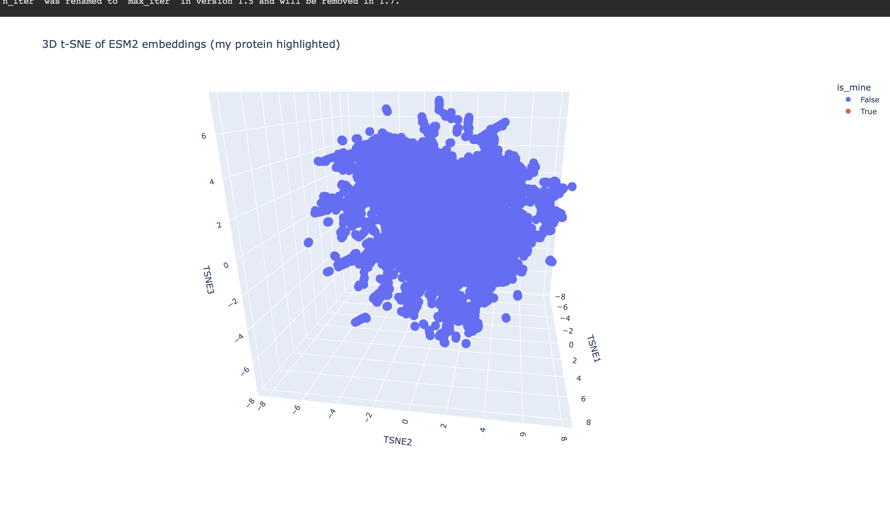
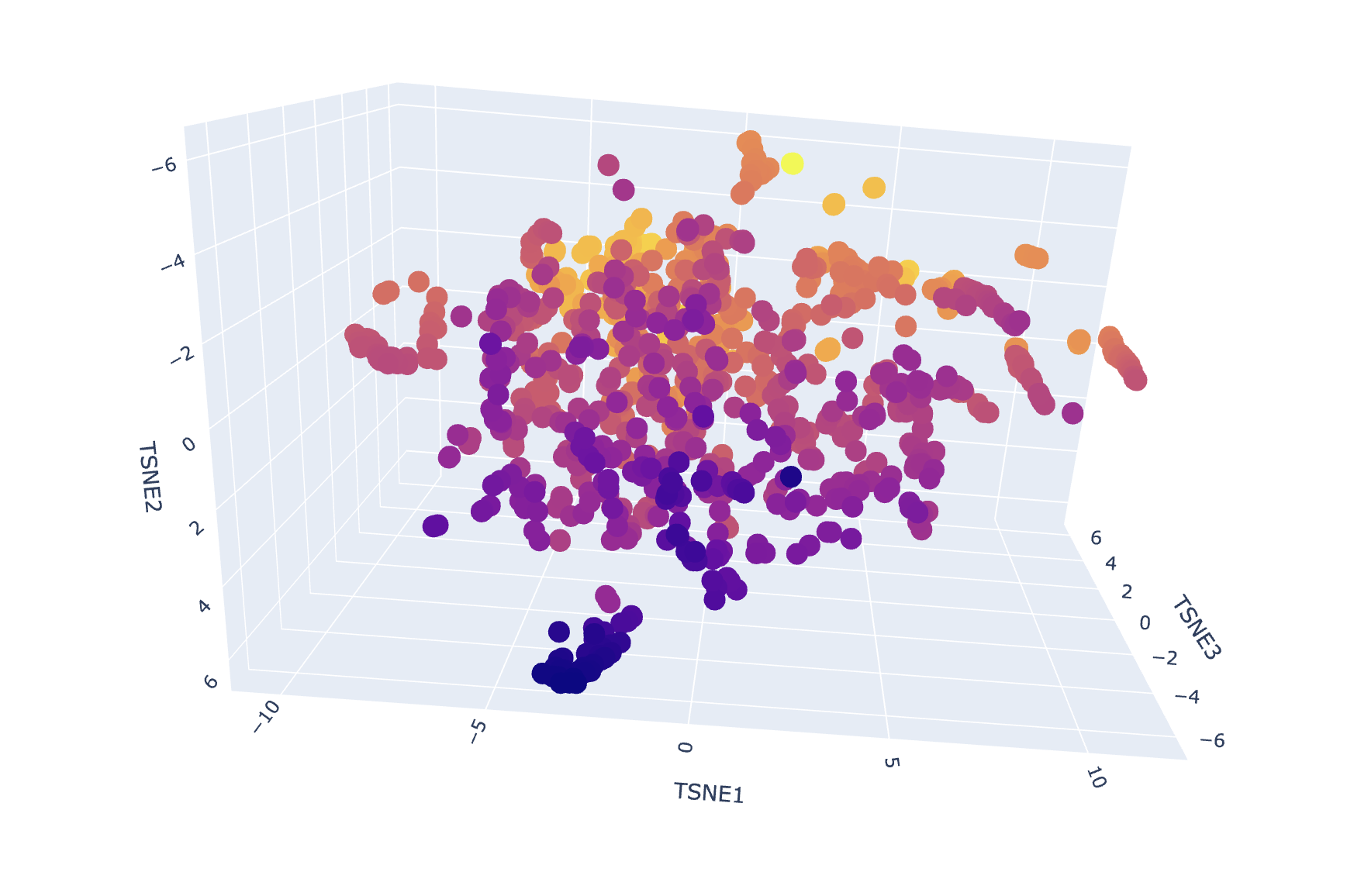
After generating mean-pooled ESM2 embeddings for the dataset, I visualized the results using a 3D t-SNE scatter plot. The dataset forms several dense regions and smaller “islands”, suggesting the embeddings capture recurring sequence/fold patterns and cluster related proteins into neighborhoods.
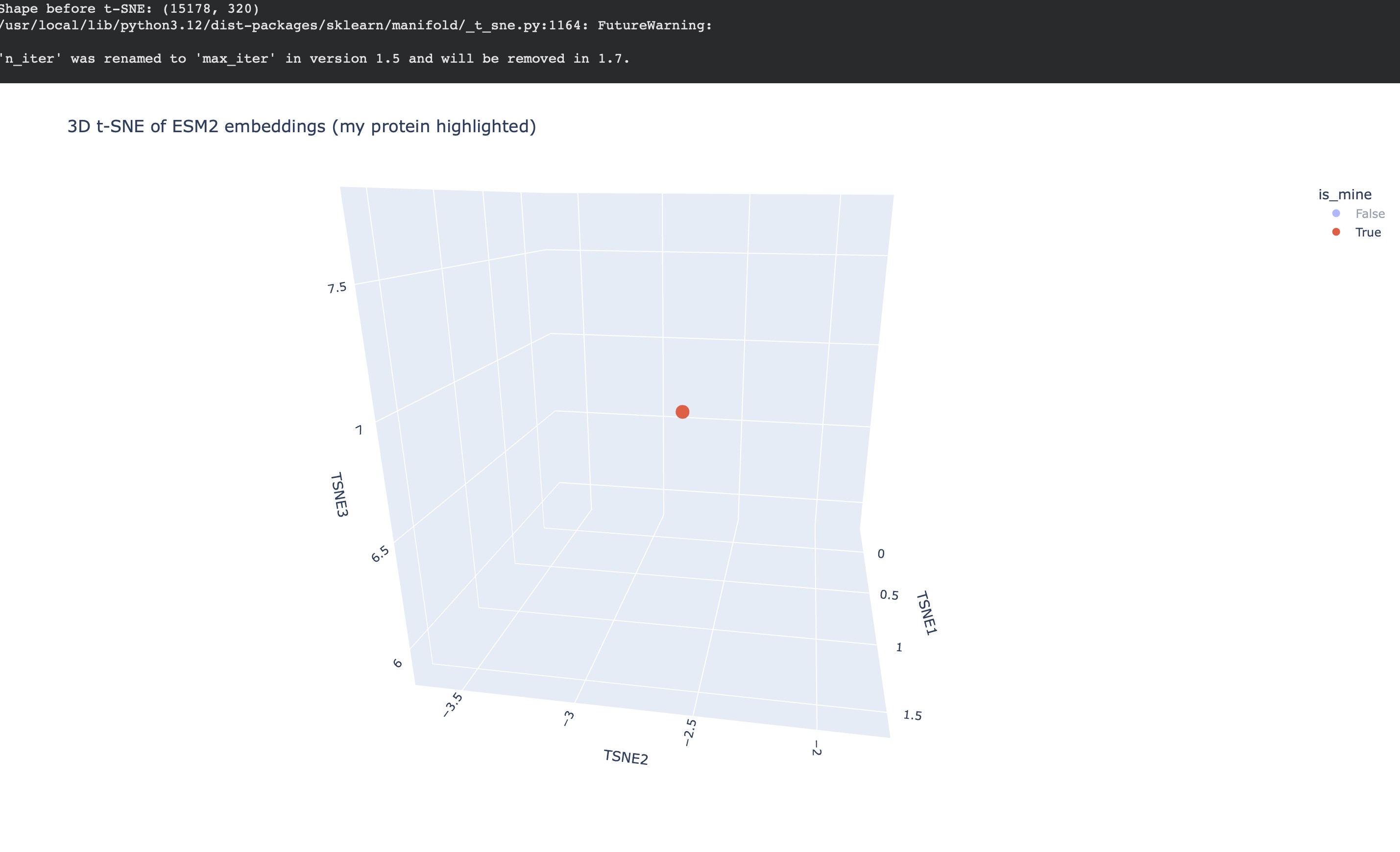 my protein in red
Placing my protein (3QXF) on the map
I then computed an embedding for my chosen protein (3QXF) using the same ESM2 embedding pipeline, appended it to the dataset, and re-ran t-SNE so that my protein appears on the same map as a highlighted point.
Nearest neighbors to 3QXF (cosine similarity in embedding space)
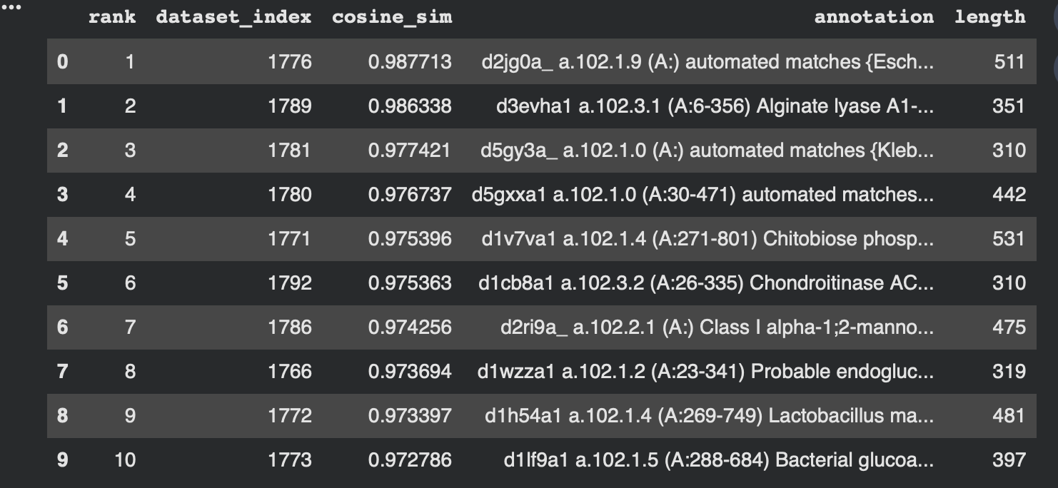
To make the neighborhood interpretation concrete, I computed cosine similarity between my protein’s embedding and every dataset embedding and extracted the top nearest neighbors. The similarities are very high (~0.97–0.99), indicating that 3QXF lands inside a tight neighborhood of closely related embeddings.
From the dataset annotations, the closest neighbors include multiple polysaccharide-active enzymes (e.g., alginate lyase, chondroitinase, and probable endoglucanase). Even though these enzymes may act on different substrates, they share common sequence/fold features typical of carbohydrate-active proteins, which likely explains why the language-model embeddings place them near each other.
Interpretation:
My 3QXF protein sits in a neighborhood enriched for carbohydrate/polysaccharide-processing enzymes, suggesting ESM2 embeddings capture higher-level similarities (shared fold/domain patterns and conserved sequence motifs) beyond exact function labels. This supports the idea that local neighborhoods in embedding space approximate “similar proteins” in terms of structure/function family.
Code snippet
- Generate mean-pooled ESM2 embeddings for the dataset sequences
- Compute my protein embedding and append it
- Run 3D t-SNE and plot
- Compute cosine similarity to retrieve nearest neighbors
C3. Protein Generation (Inverse Folding)
Picture Source:
- Post from Sergey Ovchinnikov
- Roney, Ovchinnikov et al. (2022). State-of-the-art estimation of protein model accuracy using AlphaFold. Phys. Rev. Lett. 129, 238101.
Goal
Use a fixed backbone from my chosen PDB (3QXF) to generate new sequence candidates with ProteinMPNN (inverse folding), then validate one designed sequence by folding it with ESMFold and comparing it to the native baseline.
1) ProteinMPNN: backbone → sequence candidates
I ran ProteinMPNN on PDB 3QXF, designing chain A while keeping chains B/C/D fixed in the scoring context. ProteinMPNN produced 16 candidate sequences at sampling temperature T = 0.1.
Important note about sequence length: ProteinMPNN designs only residues that exist in the PDB ATOM coordinates (i.e., modeled residues). That’s why the “native” chain segment used here is 337 aa, not the full-length annotated FASTA (which can include missing terminal residues and expression tags).
ProteinMPNN reports seq_recovery ≈ 0.51 for sample 1, meaning the designed sequence is ~51% identical to the modeled native chain segment while still being compatible with the same backbone.
2) Predicted sequence probabilities (ProteinMPNN)
ProteinMPNN also saves per-position amino-acid probabilities (distribution over 20 AAs per residue position) in:
/content/mpnn_out/probs/3QXF.npz
These probabilities can be summarized as:
- max probability per position (how confident the model is at each residue)
- entropy per position (how uncertain the model is / how many choices are plausible)
(If you haven’t made these plots yet, you can generate them with the code snippet at the end of this section and add screenshots.)
3) ESMFold validation (sequence → structure)
Native baseline (PDB-modeled chain A)
I first folded the native modeled chain-A segment (same residue range ProteinMPNN used) using ESMFold.
- Length: 337 aa
- pTM: 0.940
- Mean pLDDT: 92.291
- Output PDB:
native_chainA_6b6cf/ptm0.940_r3_default.pdb
ProteinMPNN-designed sequence (T=0.1, sample=1)
Next, I folded the ProteinMPNN-designed candidate (sample 1) with ESMFold:
- Length: 337 aa
- pTM: 0.948
- Mean pLDDT: 92.546
- Output PDB:
mpnn_sample1_bf1be/ptm0.948_r3_default.pdb
Interpretation: Both native and designed sequences have very high pTM and pLDDT, and visually they form the same compact globular fold. This suggests ProteinMPNN successfully proposed a new sequence that remains compatible with the original backbone fold.
Figures
Saved ESMFold output PDBs (native vs designed):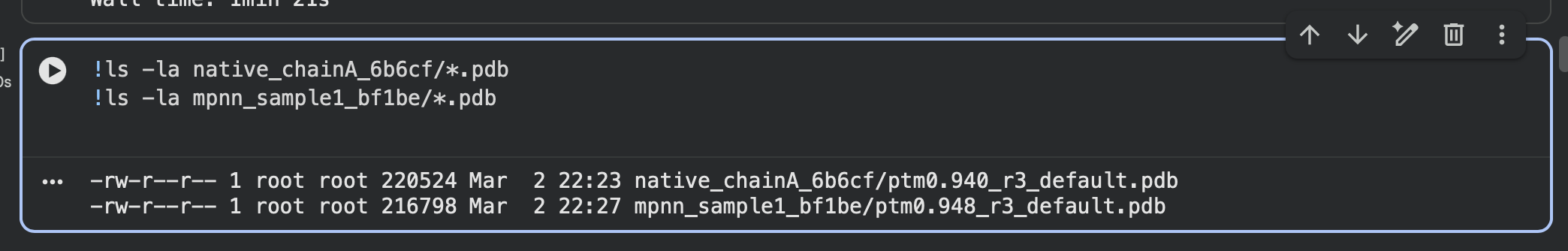
ESMFold predicted structure — Native (modeled chain A, rainbow coloring):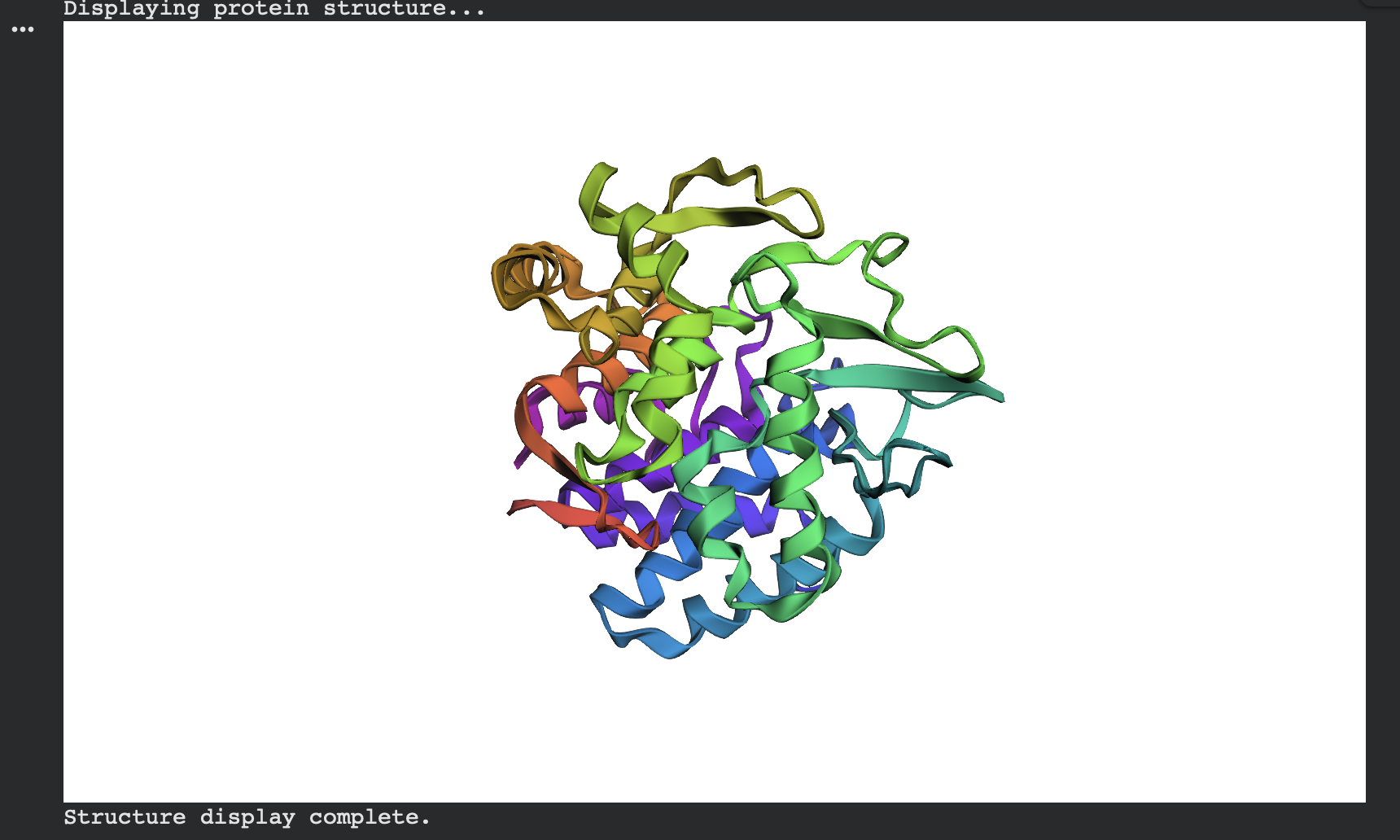
ESMFold predicted structure — ProteinMPNN sample 1 (rainbow coloring):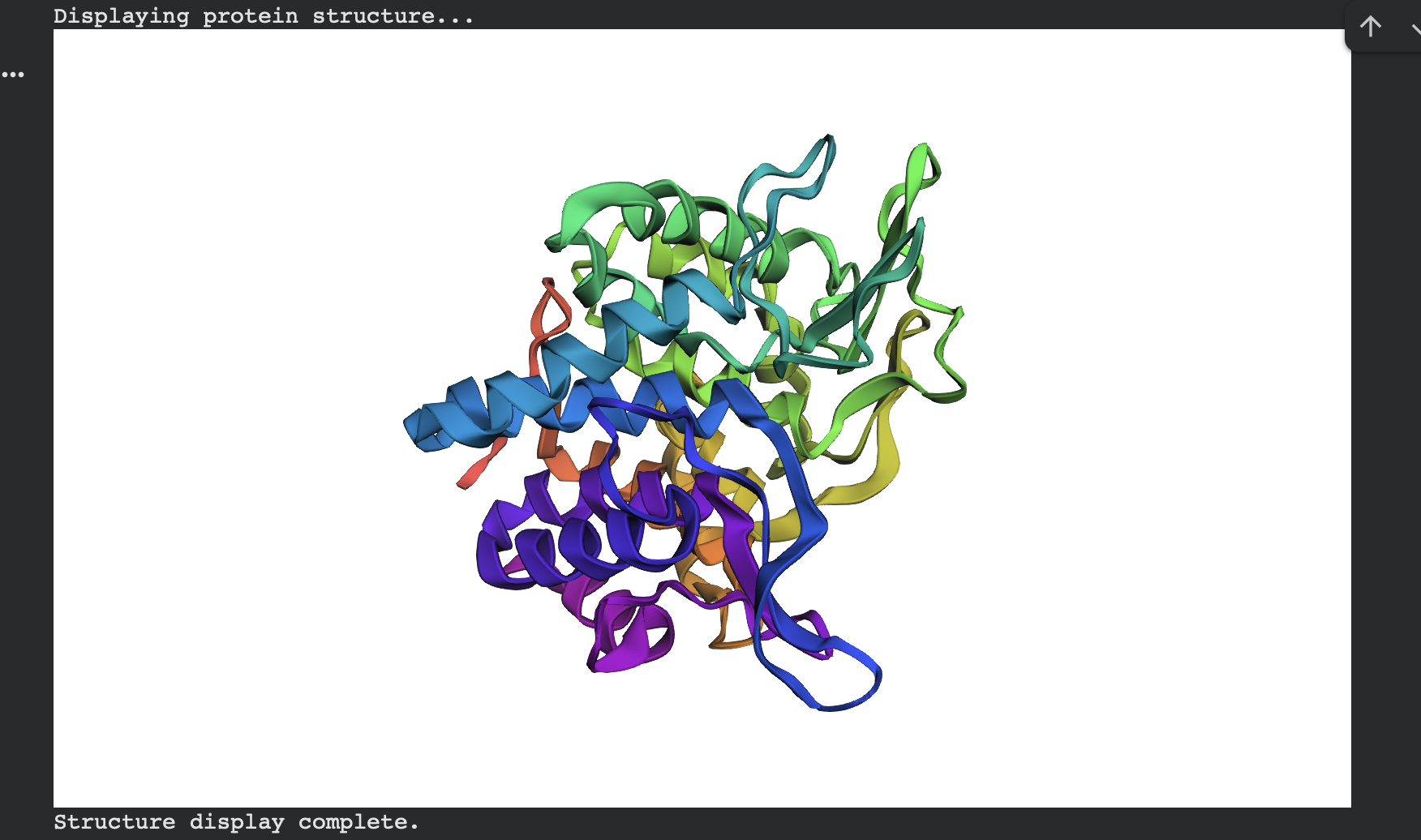
Alternate view (same prediction, different camera angle):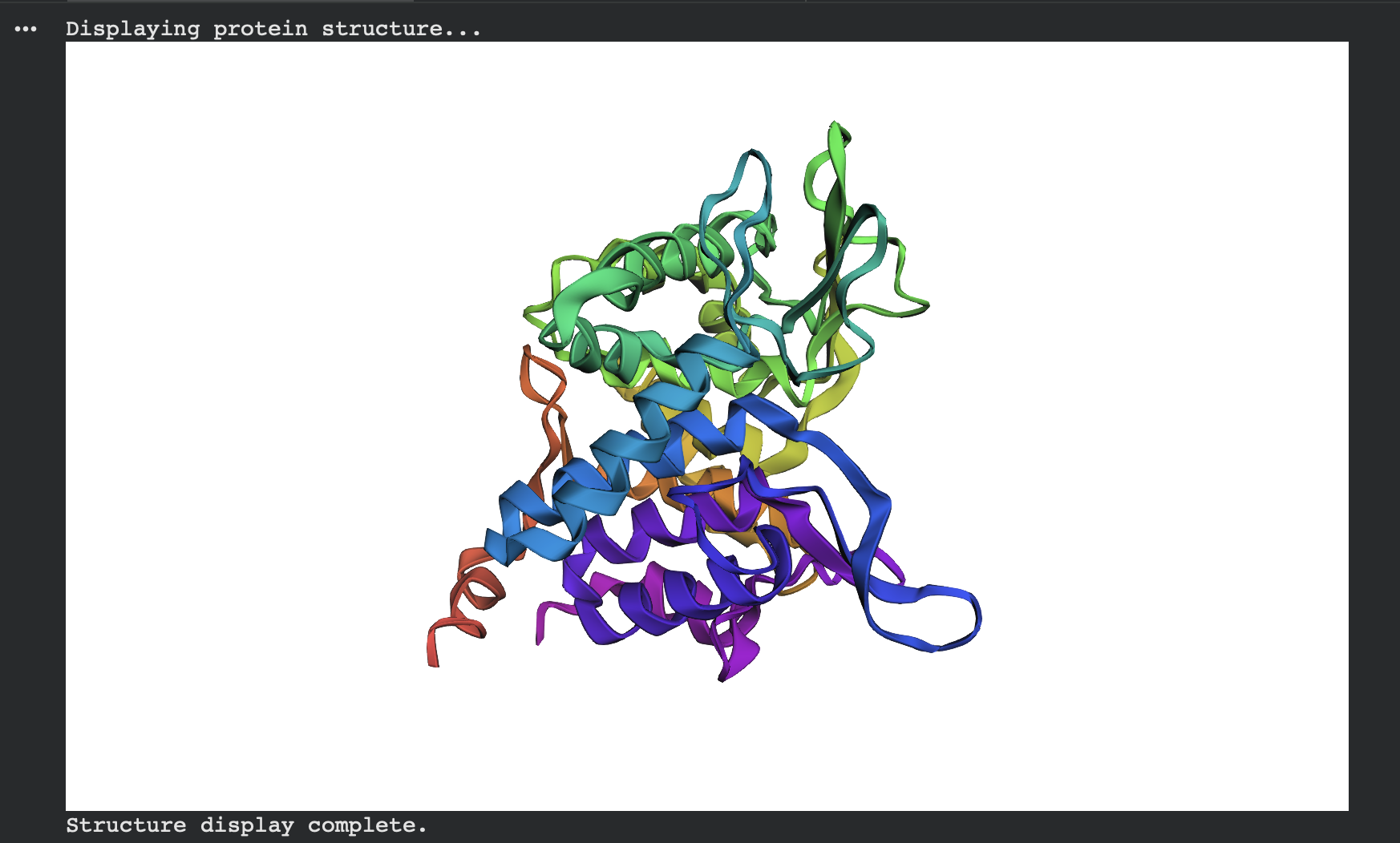
( Code to generate ProteinMPNN probability plots
Use this to create the two plots (max probability + entropy).
Inverse Folding with ProteinMPNN
For this part, I used the backbone of PDB: 3QXF and performed inverse folding with ProteinMPNN. I set the model to design chain A while keeping chains B, C, and D fixed.
ProteinMPNN generated a new sequence candidate for chain A based on the original backbone geometry. The native chain A sequence and the designed sequence were both 337 amino acids long. When I compared them, the designed sequence matched the native sequence at 175 out of 337 positions, giving a sequence identity of 51.93%. This means the model changed almost half of the residues while still proposing a sequence compatible with the same backbone fold.
The model also assigned a better score to the designed sequence than to the native one. The native score was 1.3309, while the sampled designed sequence had a score of 0.7779. Since this score reflects the model’s negative log-likelihood, the lower score suggests that ProteinMPNN considers the designed sequence highly compatible with the input backbone.
To further test the design, I folded the ProteinMPNN-generated sequence using ESMFold. The resulting predicted structure was then compared to the original 3QXF chain A structure. The comparison showed a Cα RMSD of 0.652 Å, which indicates that the predicted structure is extremely close to the original backbone. This suggests that the redesigned sequence preserves the same overall fold very well.
The confidence of the ESMFold prediction was also high. The output gave a mean pLDDT of 0.92 (with a minimum of 0.57 and maximum of 0.97), indicating that most of the structure was predicted with strong confidence.
Structural Overlay
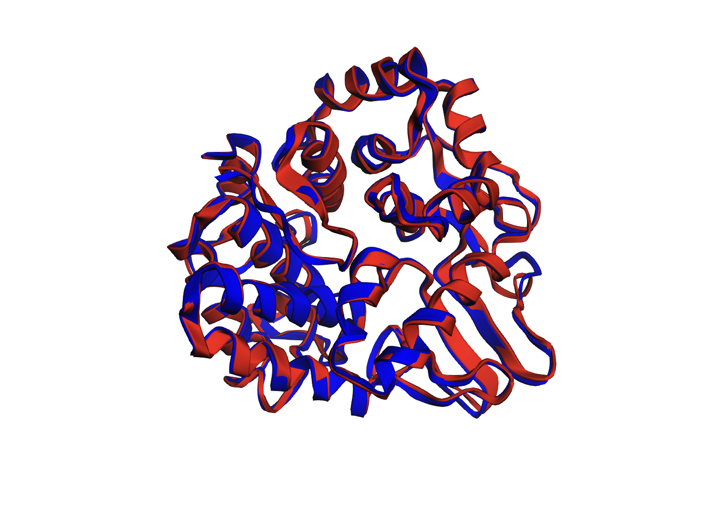
Figure 1. Overlay of the original 3QXF chain A structure and the ESMFold-predicted structure for the ProteinMPNN-designed sequence. The two structures align very closely, with only minor deviations in a few flexible regions.
Side-by-Side Comparison
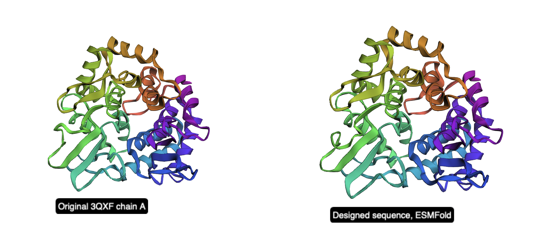
Figure 2. Side-by-side cartoon view of the original 3QXF chain A structure (left) and the ESMFold prediction of the redesigned sequence (right). The global fold is preserved, showing that the redesigned sequence remains compatible with the original backbone.
Amino Acid Probability Heatmap
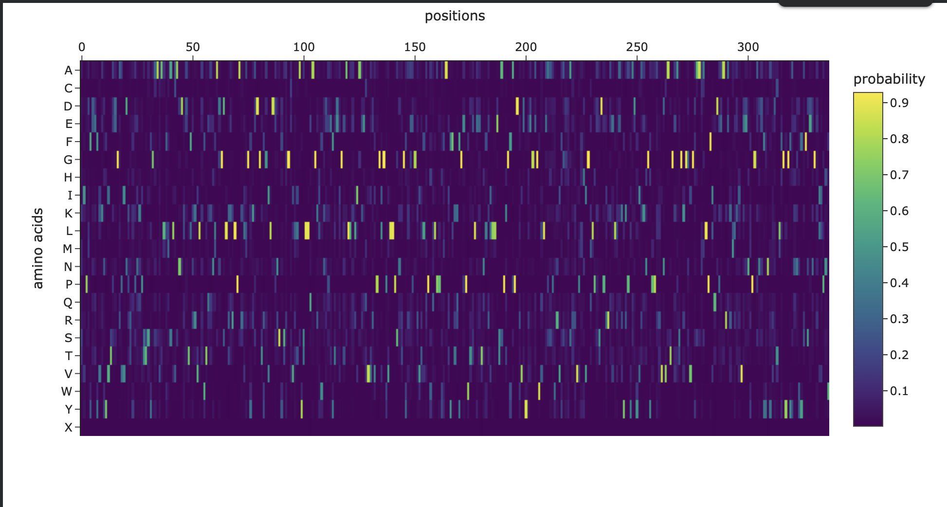
Figure 3. Amino-acid probability heatmap from ProteinMPNN showing the predicted residue probabilities at each sequence position. Bright, high-probability peaks indicate strongly constrained positions, while darker regions suggest positions that can tolerate more sequence variation.
Overall, this inverse-folding experiment shows that ProteinMPNN can generate a substantially different sequence while still preserving the original fold. Even with only about 52% sequence identity, the redesigned sequence folds back into a structure that is nearly identical to the starting backbone, demonstrating the robustness of structure-guided protein design.
Part D — Bacteriophage Engineering Proposal
Selected Goal
I propose to focus on:
- Primary goal: Increasing stability of the phage lysis (L) protein
- Secondary goal: Modulating interaction with host machinery (e.g., E. coli DnaJ)
This direction is computationally tractable and aligns with available protein design tools while still connecting to functional outcomes (lysis efficiency and phage fitness).
Rationale
The L protein is responsible for host cell lysis and is therefore a key determinant of bacteriophage replication efficiency. Improving its structural stability could:
- Increase protein lifetime inside the host
- Improve folding efficiency
- Potentially increase effective lysis activity
Additionally, modifying interactions with host proteins (e.g., DnaJ chaperone system) could alter:
- Protein degradation pathways
- Folding dynamics
- Toxicity and timing of lysis
These properties make the L protein a suitable target for computational protein engineering concepts.
Proposed Computational Approach
1. Sequence Analysis & Baseline Characterization
- Use UniProt / BLAST to identify homologs
- Generate multiple sequence alignment (MSA)
- Identify conserved vs variable regions
Goal: Identify mutation-tolerant regions
2. Structure Prediction
- Predict structure using ESMFold or AlphaFold2
Goal: Obtain structural model for downstream design
3. In Silico Mutagenesis (Protein Language Models)
- Use ESM-2 to perform:
- Deep mutational scanning (in silico)
- Likelihood scoring of mutations
Goal: To identify mutations likely to improve stability without disrupting function
4. Sequence Optimization
- Use ProteinMPNN:
- Redesign selected regions (not the full protein, to preserve function)
- Generate candidate sequences
Goal: Improve packing, stability, and foldability
5. Structural Validation
- Re-run ESMFold / AlphaFold on designed variants
- Compare:
- pLDDT (confidence)
- Structural deviations
Goal: Filter unstable designs
6. Interaction Modeling
- Use AlphaFold-Multimer:
- Model interaction with host proteins (e.g., DnaJ)
Goal: Evaluate whether mutations alter interaction in the host organism
Pipeline Schematic
Why These Tools
Protein Language Models (ESM-2):
Capture evolutionary constraints → useful for predicting tolerated mutationsProteinMPNN:
Enables structure-based redesign → improves stability via better packingAlphaFold / ESMFold:
Provide fast structural validation → essential for screening designsAlphaFold-Multimer:
Allows hypothesis testing of host–phage interactions
Together, these tools enable a pipeline from sequence to function hypothesis.
Potential Pitfalls
Lack of experimental validation
- Computational predictions may not correlate with real folding or function
Limited training data for phage proteins
- Models are biased toward well-studied proteins
- Phage-specific interactions may be poorly captured
Over-optimization risk
- Increasing stability may reduce functional dynamics needed for lysis
Conclusion
This approach focuses on stability engineering as an accessible entry point into bacteriophage design. By combining protein language models, structure prediction, and sequence redesign, it is possible to generate testable hypotheses for improved phage function, while staying within the scope of computational tools introduced in HTGAA.
References
Rives, A. et al. (2021) — Biological structure and function emerge from scaling unsupervised learning
https://doi.org/10.1101/622803Lin, Z. et al. (2023) — ESMFold: Evolutionary-scale prediction of atomic-level protein structure with a language model
https://www.science.org/doi/10.1126/science.ade2574Jumper, J. et al. (2021) — Highly accurate protein structure prediction with AlphaFold
https://www.nature.com/articles/s41586-021-03819-2Dauparas, J. et al. (2022) — Robust deep learning–based protein sequence design using ProteinMPNN
https://www.science.org/doi/10.1126/science.add2187