I’m an industrial designer currently pursuing a MDE Degree at Harvard. In my practice, i’m focused on multidisciplinary research - utilizing digital & traditional fabrication methods, computational methodologies, philosophy and critical thinking - I observe, dismantle and reconstruct the concepts I’m working with, using whimsical and subversive motives to question the ordinary and unearth speculative near-futures. I believe that design is a tool to address social , environmental & economic wickedities, advancing us towards a more holistic and responsible approach towards just being and being just.
1. First, describe a biological engineering application or tool you want to develop and why.
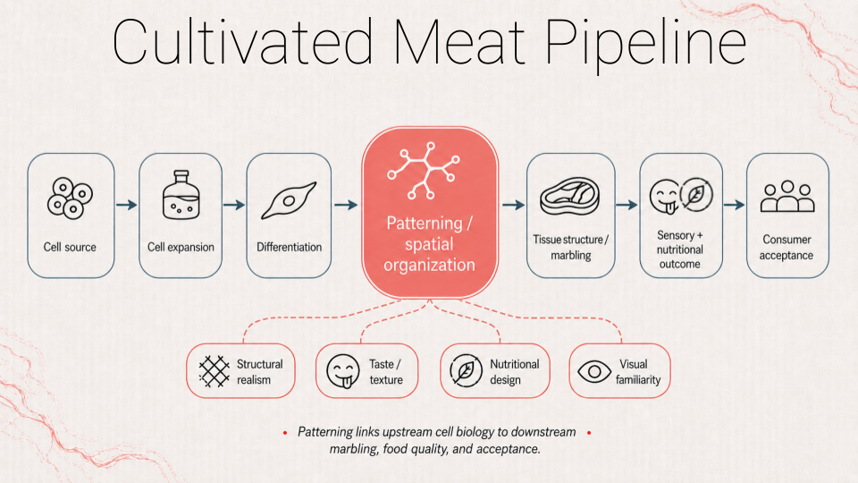
I’m curious about cellular agriculture and lab-grown meat. in this project im proposing to develop a living, light-activated scaffold that produces and spatially distributes oxygen inside a growing tissue. this is one of the needed early steps toward making a thick, steak-like cut rather than thin sheets or ground meat. Today, animal cells grown for food struggle beyond a few millimeters because oxygen and nutrients don’t diffuse well. the interior becomes starved and dies unless you add complex and expensive hardware. My project reframes that bottleneck as a biological engineering opportunity: a biofabricated “breathing” matrix that couples geometry + metabolism so that illumination drives localized oxygen generation and makes it visible and tunable. In this course’s context it would be explored as a living installation: a translucent scaffold whose oxygen field can be visualized in real time under light/dark cycles, producing both data and an intuitive, aesthetic demonstration of how engineered living materials might reduce reliance on expensive hardware in future cultivated-meat systems.
2. Describe one or more governance/policy goals related to ensuring that this application or tool contributes to an “ethical” future, like ensuring non-malfeasance (preventing harm). Break big goals down into two or more specific sub-goals.
Governance policy goal #1: ensuring Biosafety and non-malfeasance
Make sure the system can’t cause harm to people, ecosystems, or lab staff through accidental release, contamination, or unsafe handling.
Making sure every engineered organism used in the project is not viable outside of the controlled lab conditions.
Contamination monitoring and incident reporting standards for all project related activities in the wet lab.
Use ‘Low Risk’ Chassis Organisms and avoid incorporating traits that increase survivability of harmful actions.
Governance policy goal #2: maximize public benefit
directing this tool toward clear societal value—lowering barriers to safer, more resource-efficient cellular agriculture research and accelerating pathways to scalable cultivated meat.
Define ‘Constructive Use’ criteria and require study to explicitly show qualitative improvement over one of the following criteria : lower resource use, improving oxygen diffusion limits, reducing complexity of tissue cultivation, reducing cost of tissue cultivation.
Encourage standardized open-source documentation for non-sensitive aspects like negative results and measurement methods.
Ensure this tool’s benefits are broadly shared rather than concentrated, and that people retain meaningful choice and informed consent.
cultural and livelihood impacts: include early stakeholder perspectives (food cultures, labor/farming communities) to reduce the risk that “technical success” drives social harm or displacement.
if such a risk is assesed as high, co-develope a slow transition plan.
3. Describe at least three different potential governance “actions” by considering the four aspects below (Purpose, Design, Assumptions, Risks of Failure & “Success”).
Action 1: Project specified containnment regime
Purpose: Replace generic lab norms with a project-specific containment regime so accidental release and unsafe handling are structurally less likely.
Design: A mandatory SOP covering labeling, storage, transport, and validated inactivation/disposal for every culture/run. chain-of-custody log for strains and materials.
Assumptions: Containment does not undermine biological performance.
Risks: Failure - checkbox compliance or incomplete logs, resulting in bad lab norms and culture. Success risk - issue of a compliance-overhead that will evemtually become a barrier for smaller teams unless tooling/templates reduce burden.
Action 2: Pre-registered public-benefit targets
Purpose: Ensure the work advances constructive uses by tying it to explicit, testable public-benefit goals rather than novelty.
Design: Before experiments, declare 1–2 primary public-benefit targets (reduced process complexity/reduced resource use) and define how they will be evaluated. after, conduct a brief impact evaluation including tradeoffs and limits.
Assumptions: Labs track real constraints; teams won’t optimize for non-beneficial metrics.
Risks: Failure - metric gaming or proxies that don’t translate. Success risk - the encourageing or incentivizing a ‘follower’ culture where the first metrics to have consenseus are repeated as defaults.
Action 3: stakeholder review & benefit-sharing
Purpose: Ensure “success” does not override cultural values, informed consent, or fairness in who benefits from the technology.
Design: A stakeholder checkpoint with at least two external perspectives (labor/farming and food culture/ethics) plus explicit benefit-sharing commitments (open standards, non-exclusive licensing norms, accessible documentation, and clear communication of uncertainties to support informed choice).
Assumptions: Early stakeholder engagement surfaces blind spots. benefit-sharing commitments foster trust between community and research/venture.
Risks: Failure risk -tokenism or performative consultation. Success risk - added friction slows iteration—but that is an intentional tradeoff to protect autonomy and prevent concentrated capture.
Action 4: responsible release of documentation
Purpose: Maximize reproducibility and shared learning while reducing misuse risk.
Design: Two publication layers: Open (concept, results, non-sensitive documentation) and Restricted (step-by-step replication details and other speceficities). an external mechanism decides classification of research documents. access to the Restricted layer will be granted by same mechanism.
Assumptions: Sensitive details can be identified; restriction won’t destroy scientific value.
Risks: Failure risk - misassuming the layer definitions as too open (misuse) or too closed (no benefit). Success risk - restricted knowledge becomes a chokepoint that concentrates power and limits equitable access.
Score (from 1-3 with, 1 as the best) each of your governance actions against your rubric of policy goals.
Drawing upon this scoring, describe which governance option, or combination of options, you would prioritize, and why. Outline any trade-offs you considered as well as assumptions and uncertainties.
I would prioritize a combined governance package aimed at two audiences:
First would be an institutional biosafety governance body (such as an IBC) and the second would focus on field-facing actors (research funders, journals, and cultivated-meat research networks). The core package is Action 1 (Containment Regime), Action 2 (Pre-registered public-benefit targets), and Action 3 (Stakeholder review & benefit sharing). I would start with Action 1 because it most directly reduces non-malfeasance risks (accidental release, unsafe handling, or unmanaged contamination). Action 2 ensures the project is oriented toward constructive use by requiring explicit evidence of benefit rather than novelty alone. Action 3 is prioritized early because success in this domain can create downstream social impacts—such as concentration of ownership or displacement pressures—so stakeholder input and benefit-sharing commitments are necessary to protect autonomy and legitimacy.
The primary trade-off is speed and ease of iteration vs. safety, accountability, and equity. These actions add overhead (documentation, evaluation, review), and if implemented too rigidly they could become barriers for smaller teams. the assumption is that this can be mitigated with lightweight templates and clear defaults. A key uncertainty is whether lab-scale proxies for oxygen distribution translate to real thick-tissue outcomes. Action 2 should make a clear and defined outline through central—pre-registering of what counts as improvement, to structured and goal-oriented claims rather than post-hoc storytelling. Overall, this prioritized set aims to make the project safe by default, oriented toward public benefit, and socially accountable if it succeeds.
Nature’s machinery for copying DNA is called polymerase. What is the error rate of polymerase? How does this compare to the length of the human genome. How does biology deal with that discrepancy?
Polymerase makes about 1 error per 106 bases. The human genome is about 3.2×10⁹ bp, so a genome-length copy would imply roughly ~3,200 errors. Biology closes that gap by layering proofreading and post-replication mismatch repair on top of polymerase.
How many different ways are there to code (DNA nucleotide code) for an average human protein? In practice what are some of the reasons that all of these different codes don’t work to code for the protein of interest?
Because many amino acids have multiple equivalent codons, the number of possible DNA sequences encoding the same protein is huge. In practice, many variants fail because the codon choice will change translation efficiency and because sequence composition changes mRNA structure.
Dr. LeProust’s Questions:
What’s the most commonly used method for oligo synthesis currently?
The most common method is solid-phase phosphoramidite chemical synthesis. It builds DNA one nucleotide at a time on a solid support through repeated cycles (coupling, capping, oxidation, deblock).
Why is it difficult to make oligos longer than 200nt via direct synthesis?
Because each added base requires another chemical cycle, small inefficiencies and side reactions add-up over hundreds of cycles.
Why can’t you make a 2000bp gene via direct oligo synthesis?
A 2000 bp gene would require ~2000 sequential synthesis cycles, making correct full-length yield very low because errors and truncations will become significant along the process.
Prof. Church’s Question:
Using Google & Prof. Church’s slide #4 : What are the 10 essential amino acids in all animals and how does this affect your view of the “Lysine Contingency”?
The EAAs in all animals are Arginine, Histidine, Isoleucine, Leucine, Lysine, Methionine, Phenylalanine, Threonine, Tryptophan, and Valine.
To my understanding ‘The Lysine Contingency’ was a strategy in the ‘Jurassic Park’ fiction implemented by Henry Wu to disable dinosaurs’ ability to create Lysine by themselves, thus forcing them to obtain it through supplements provided by the park, or die.
Since I now know no known-animal has the ability to self-produce the EAA Lysine, this renders as complete nonsense - because the dinosaurs did not have the ability to create the Lysine in the first place. The concept of a kill-switch however, still stands valid as a bio-safety measure.
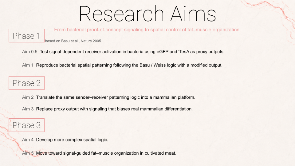
Identify at least one aspect of your project that you will measure.
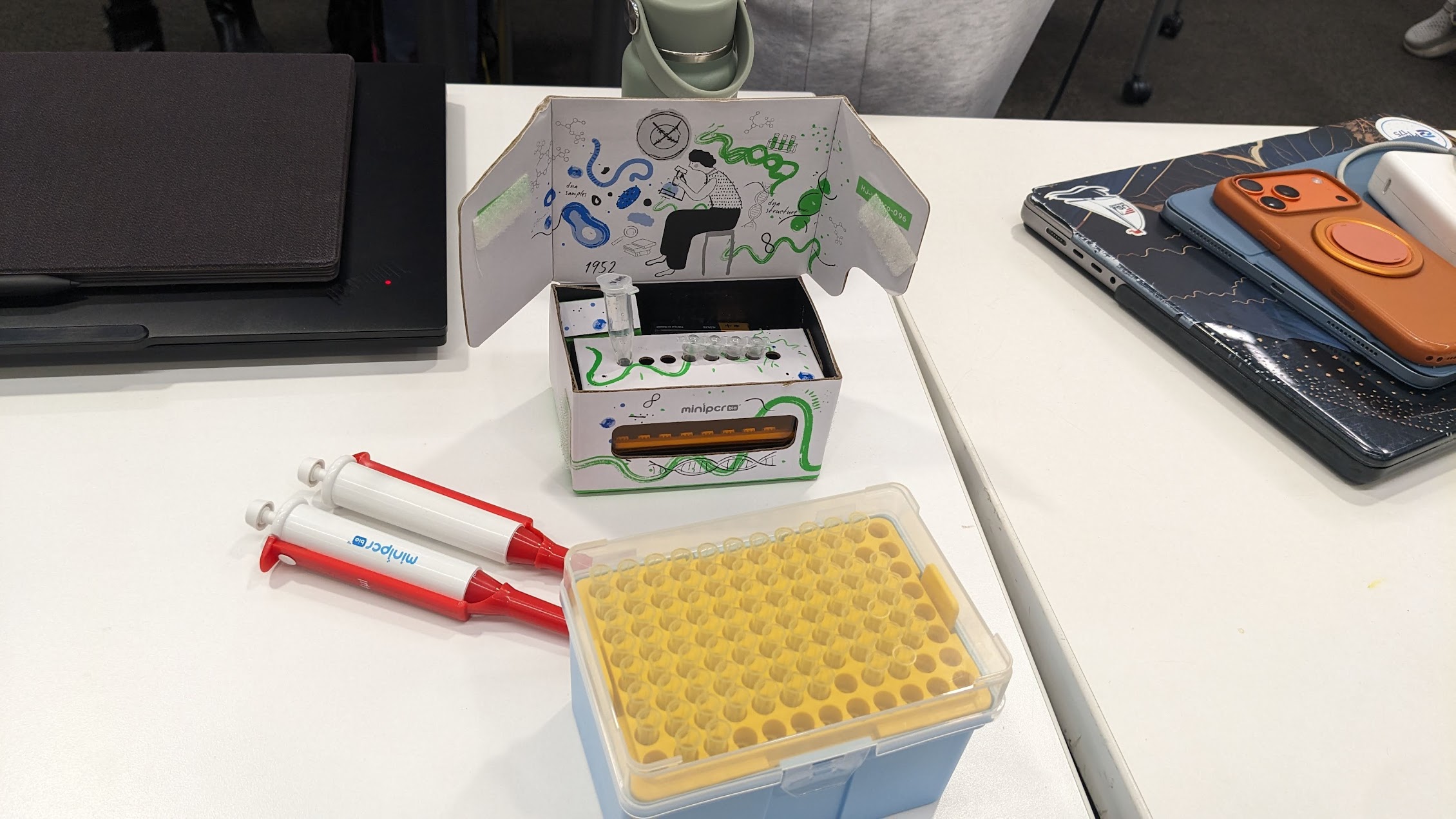
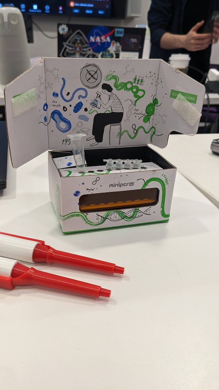
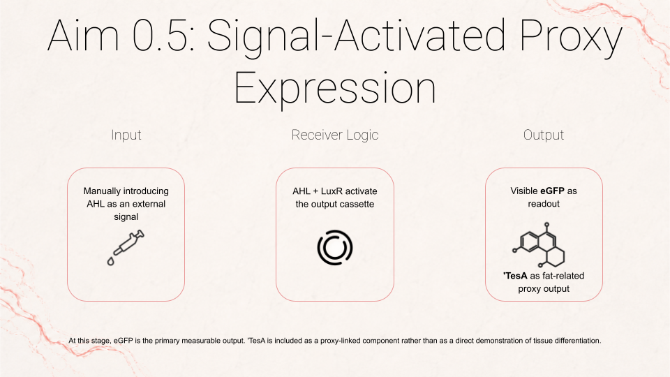
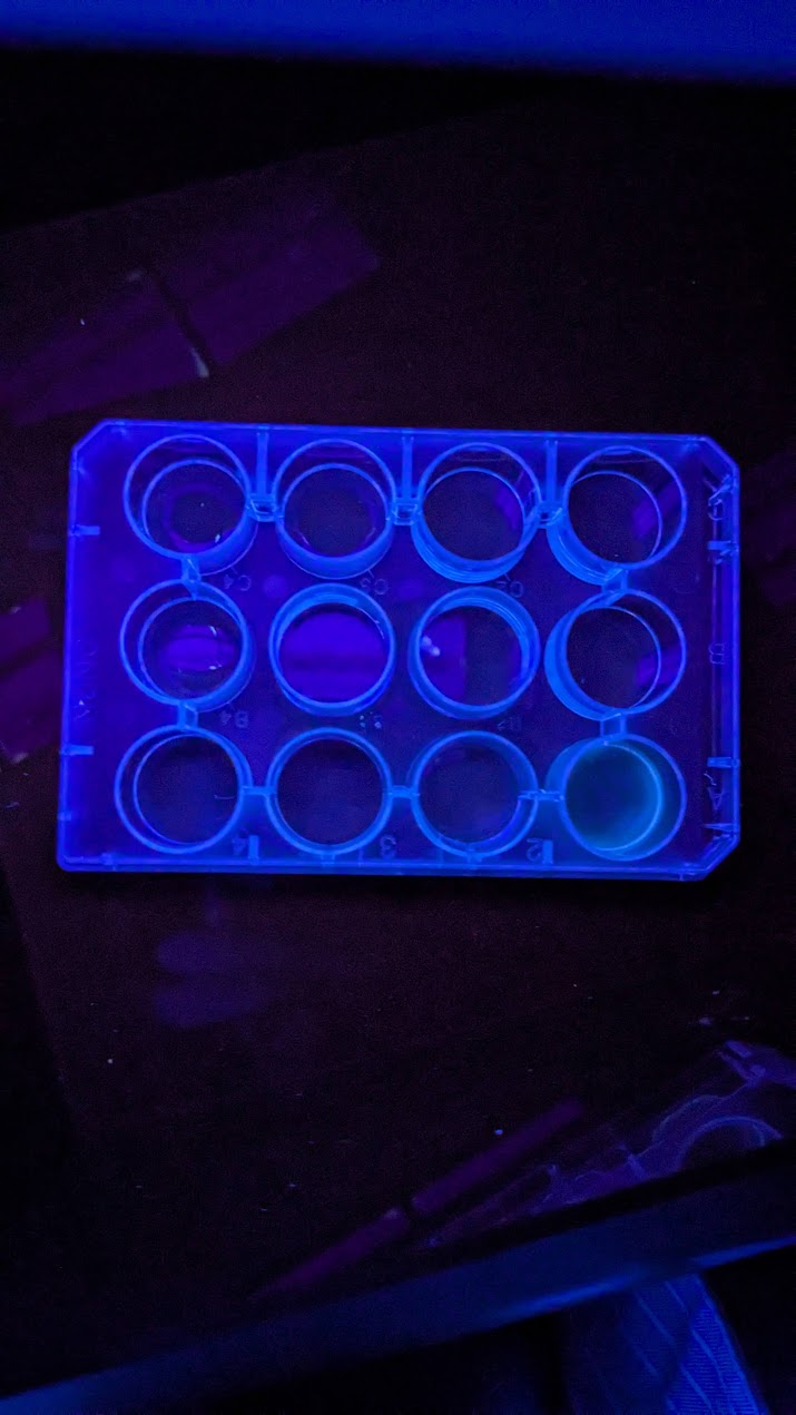
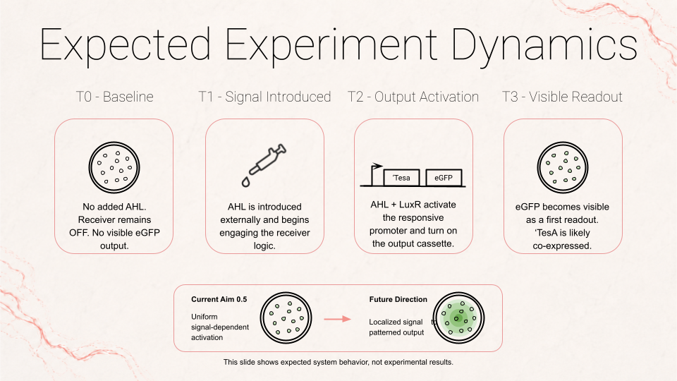
One aspect I will measure is the spatial response of receiver cells to a signaling source, by quantifying reporter intensity as a function of distance from sender cells. Another aspect I will measure, especially for Aim 0.5, is the activation of the fat-related proxy, using eGFP fluorescence as a readout for co-expression of ‘TesA in the receiver cells. Together, these give me two measurable outputs: whether the system forms a real gradient in space, and whether that gradient is successfully coupled to a fat-related expression program.
Describe all of the elements you would like to measure, and furthermore describe how you will perform these measurements. What are the technologies you will use?
I would like to measure the following metrics:
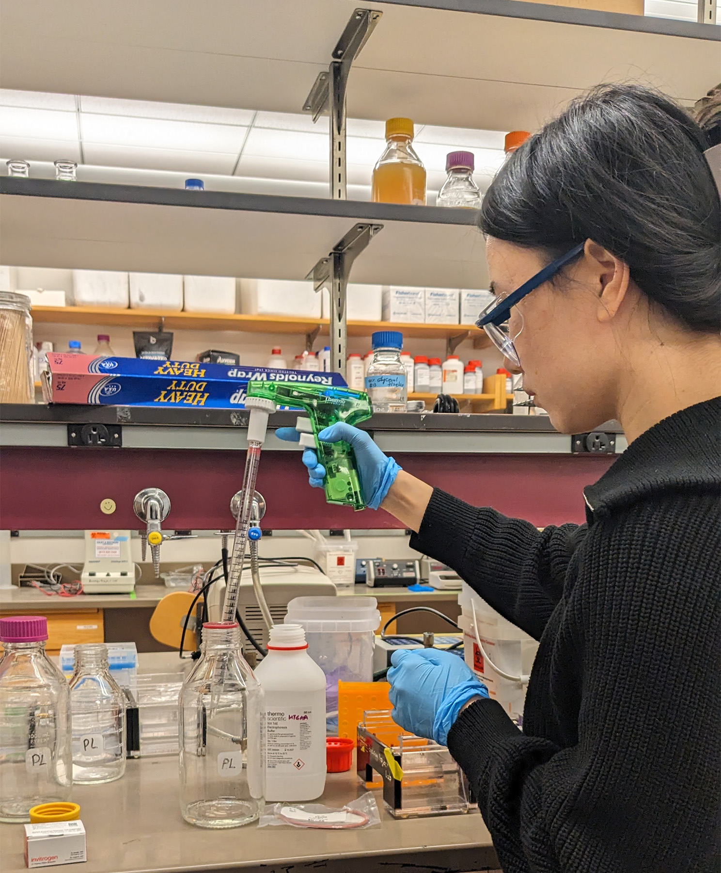
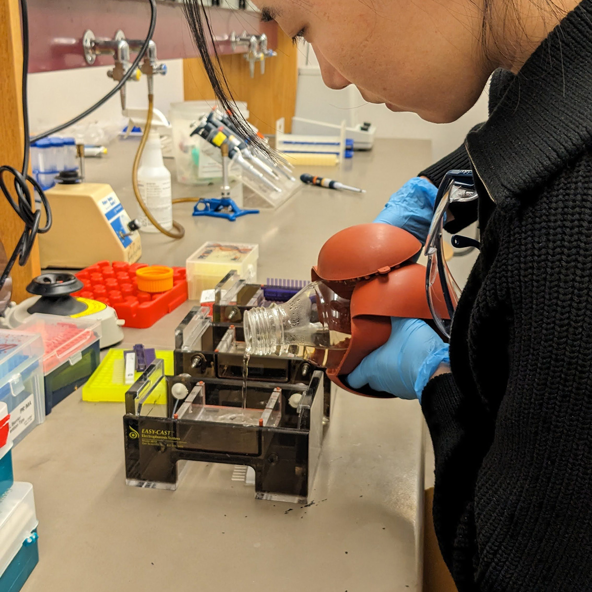
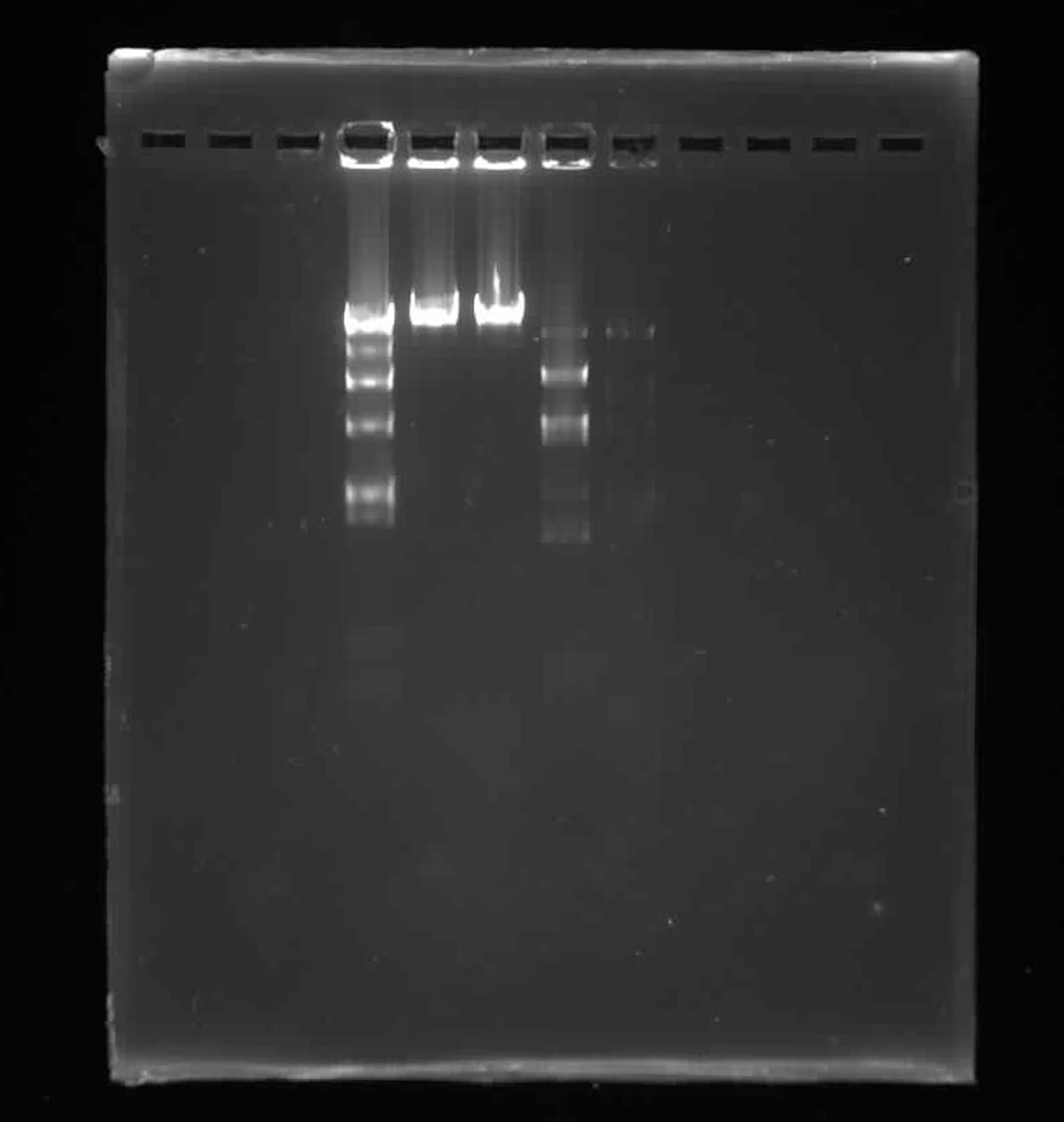
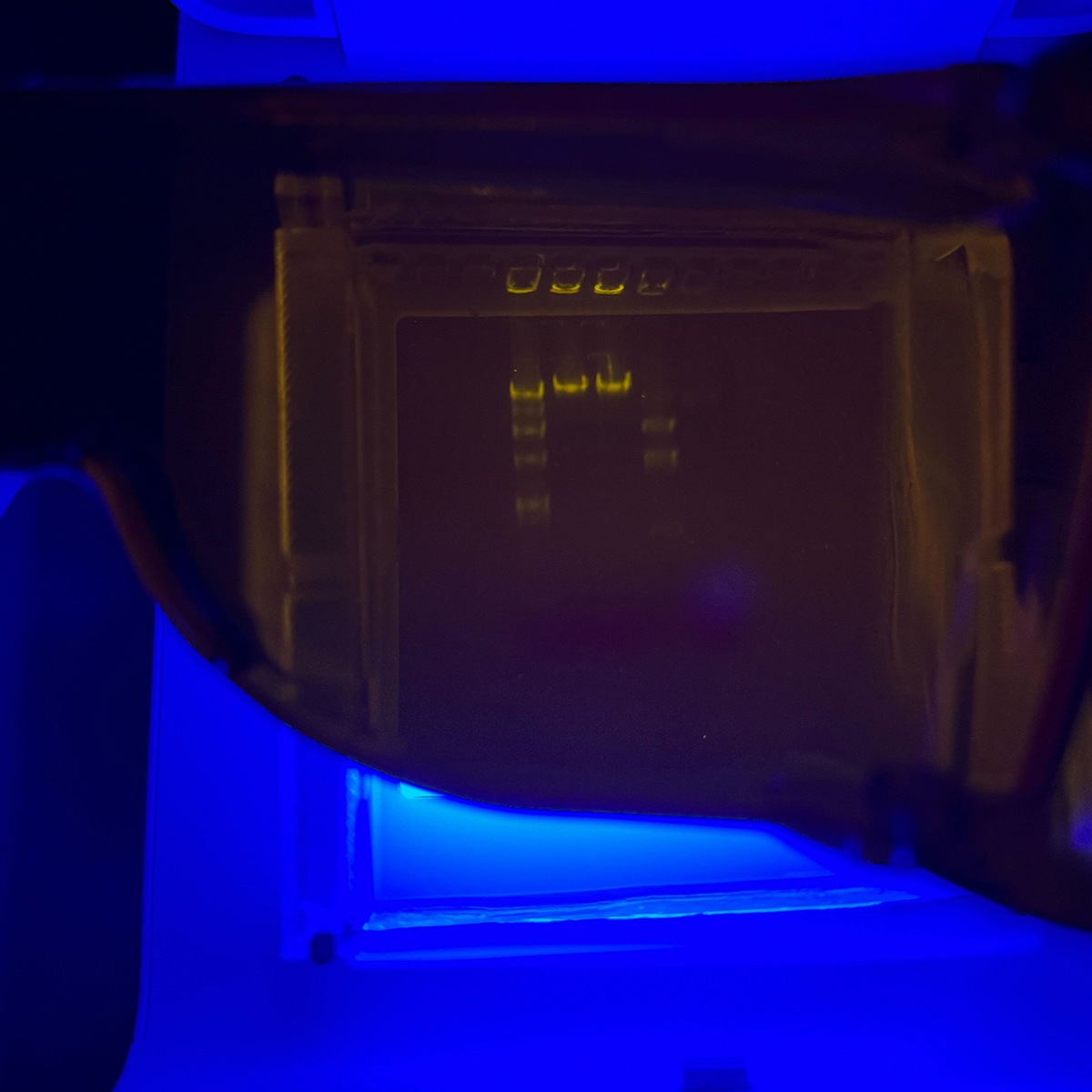
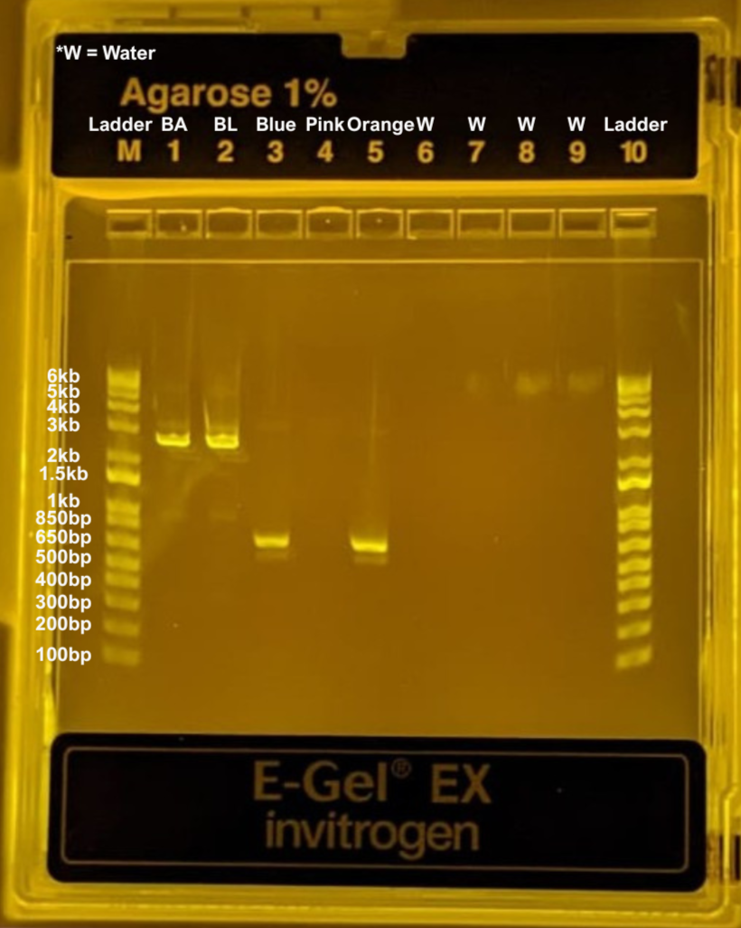
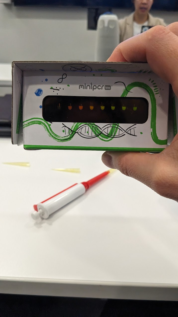
a. I will confirm fragment sizes during cloning and validation steps to validate and check whether the expected DNA products are present using gel electrophoresis.
b. Receiver activation by tracking eGFP fluorescence intensity over time and, when possible, as a function of distance from sender cells using video timelapse. This would let me see whether the circuit is simply on or off, and whether it produces any spatial pattern rather than a uniform response. I would compare this against controls such as receiver-only culture.
c. ‘TesA expression, since the conceptual point of Aim 0.5 is to link fluorescence to a fat-related expression program. I would ideally use a protein-level assay kit such as an 4–20% Mini-PROTEAN® TGX™ Precast Gel to check whether a protein of the expected size is being produced. In principle, mass spectrometry could also be used to confirm protein identity more precisely, although for the scope of Aim 0.5 it would likely be a more advanced method than I strictly need.
d. Whether expression of ‘TesA corresponds to any increase in free fatty acid production (FFA). Even a coarse measurement here would strengthen the experiment, because it would move the result toward actual biological activity. For this I could use a free fatty acid assay kit / colorimetric assay such as this MAK466 Sigma-Aldrich Free Fatty Acid assay kit for a crude evaluation.
e. I would monitor culture performance: growth, viability, and environmental parameters like media conditions, temperature, and possibly pH. Since both the sender and receiver rely on engineered expression, these background conditions matter because weak growth or excessive burden could distort the interpretation of fluorescence or proxy expression. I plan to use standard microbiology measurements such as optical density, growth observations, and controlled culture conditions.
Week 11: Bioproduction & Cloud Labs
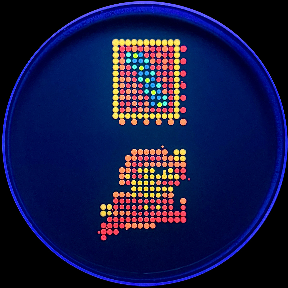
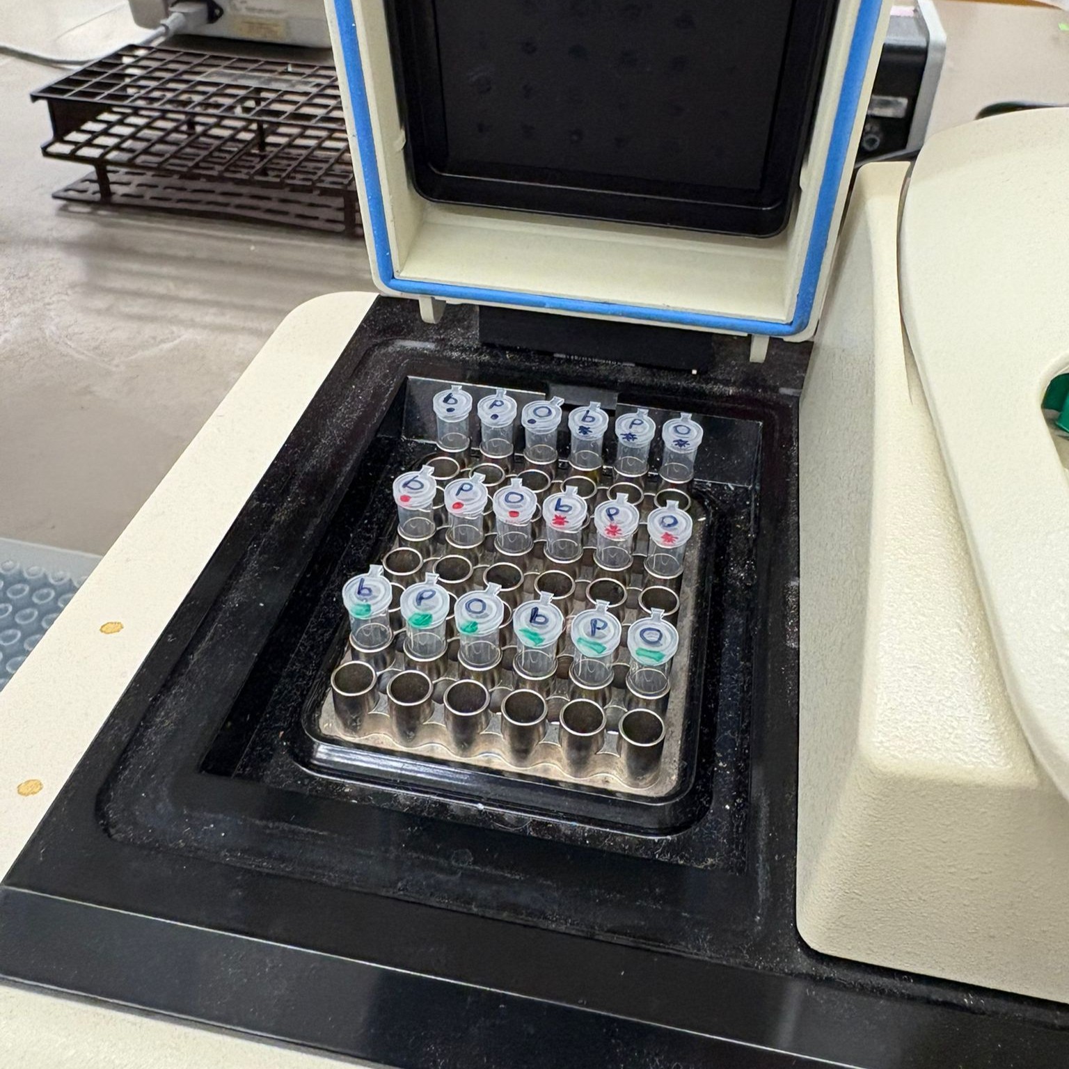
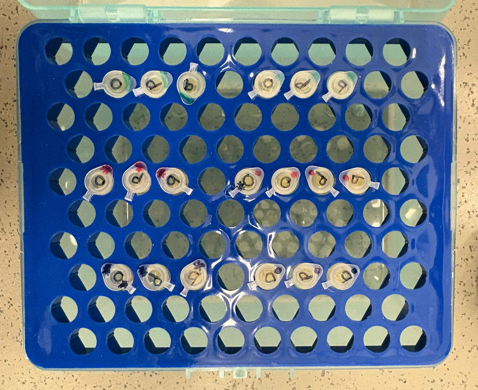
Part A: The 1,536 Pixel Artwork Canvas | Collective Artwork
What I contributed to the community bioart project
I looked up the final artwork, but I could only find the second version, which unfortunatley I could not contribute to in time. Even so, I found the project very compelling. Since I missed this round’s contributions, and respecting the week 11 homework description would be very happy to join HTGAA as a TA next semester!
What I liked about the project
What I liked most was its collaborative r/place-like quality and the nod to an original cultural phenomenon shaped by online communities. In the context of this course, that idea became even more meaningful, because it was extended through real distributed participation: people in different locations around the world were all taking part in the same collective experiment. I appreciated how the project made that network visible through a shared visual output.
What could be improved for next year
One possible improvement would be to expand the expressive range of the system by introducing more colors, more wells, or even a custom color-mixing interface. That could make the final artifact richer and allow participants to contribute with more nuance and variation.
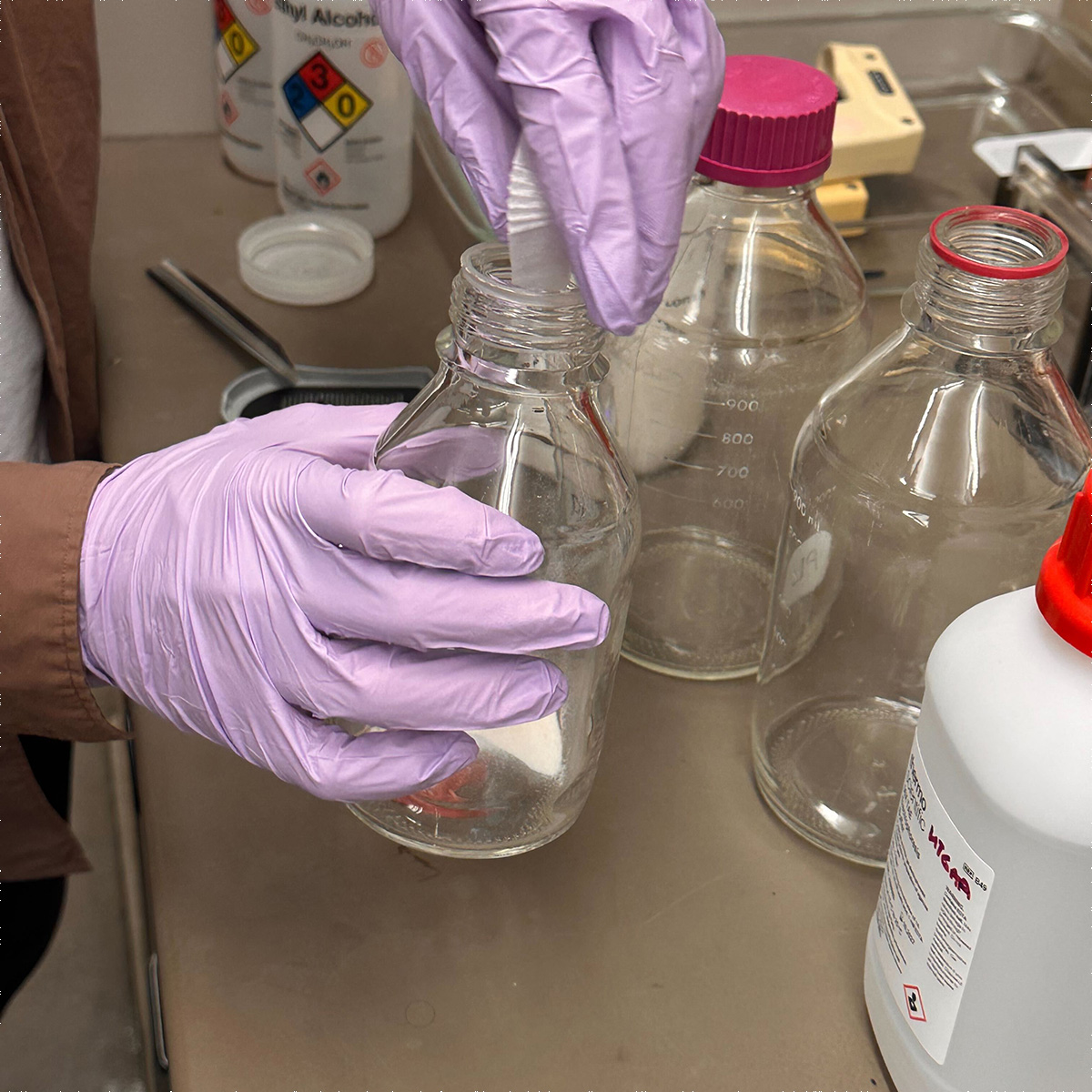
Part B: Cell-Free Protein Synthesis | Cell-Free Reagents
Roles of each component in the cell-free reaction
E. coli Lysate
BL21 (DE3) Star Lysate (includes T7 RNA Polymerase) The lysate provides the core molecular machinery needed for cell-free transcription and translation, including ribosomes, tRNAs, metabolic enzymes, and translation factors. Because this lysate comes from BL21 (DE3) Star, it also includes T7 RNA polymerase, which transcribes genes placed under a T7 promoter.
Salts / Buffer
Potassium Glutamate Potassium glutamate helps recreate an intracellular-like ionic environment and supports ribosome and enzyme function during transcription and translation. It is often used as a major salt in bacterial cell-free systems because it better mimics cytoplasmic conditions than simple chloride salts.
HEPES-KOH pH 7.5 HEPES-KOH is the buffering system that keeps the reaction near a stable physiological pH. Maintaining pH is important because both transcription and translation enzymes are sensitive to acid/base changes over the course of the reaction.
Magnesium Glutamate Magnesium is an essential cofactor for many enzymes in the reaction, especially RNA polymerase, ribosomes, and enzymes involved in nucleotide handling. If magnesium is too low or too high, the reaction can fail or become inefficient, so it is one of the most critical tuning parameters in CFPS.
Potassium phosphate monobasic This phosphate salt helps contribute to the buffering and ionic balance of the reaction. Together with the dibasic form, it helps stabilize pH and phosphate availability in the system.
Potassium phosphate dibasic This works with monobasic phosphate as part of a conjugate buffer pair. It helps maintain pH stability and contributes to the chemical environment needed for efficient enzyme activity.
Energy / Nucleotide System
Ribose Ribose serves as a carbon source that can support nucleotide and energy metabolism in longer-running cell-free reactions. It is especially relevant in systems that regenerate resources over time rather than relying only on a single high-energy phosphate donor.
Glucose Glucose provides an additional metabolic energy source that can feed endogenous enzymatic pathways in the lysate. In longer reactions, it helps sustain ATP regeneration indirectly and support continued protein production.
AMP AMP is a nucleotide monophosphate precursor that can be recycled into higher-energy nucleotide forms in extended energy-regeneration systems. In this setup it supports rebuilding the nucleotide pool rather than supplying ATP directly.
CMP CMP is a precursor for cytidine nucleotide regeneration and helps replenish the RNA-building pool needed for transcription. It is part of the lower-energy nucleotide set used in longer-duration reactions.
GMP GMP supports regeneration of guanosine nucleotide pools used in RNA synthesis and other reaction processes. Like the other monophosphates, it is part of a resource-efficient long-duration system.
UMP UMP is the uridine nucleotide precursor used to support RNA synthesis after regeneration into higher-energy forms. Its inclusion helps sustain transcription over longer reaction times.
Guanine Guanine is a free nucleobase that can feed salvage pathways in the lysate to help replenish guanine nucleotide pools. It supports longer-term reaction economy by contributing to nucleotide regeneration.
Translation Mix (Amino Acids)
17 Amino Acid Mix This mixture provides most of the amino acids needed as building blocks for protein synthesis. They are consumed directly by the ribosome as the target protein is translated.
Tyrosine Tyrosine is often added separately because of solubility or stability issues in concentrated amino acid mixes. It serves the same role as the others: supplying a required amino acid for protein synthesis.
Cysteine Cysteine is also commonly handled separately because it is chemically more reactive and less stable in stock solutions. It is required for translation of proteins containing cysteine residues and can also influence redox-sensitive folding contexts.
Additives
Nicotinamide Nicotinamide supports metabolic cofactor balance because it is related to NAD-dependent biochemical pathways. In cell-free reactions, additives like this can help maintain metabolic activity and improve reaction longevity.
Backfill
Nuclease Free Water Nuclease-free water is used to bring the reaction to its final volume without introducing DNases or RNases that could degrade templates or transcripts. It acts as the clean solvent base for the reaction mixture.
Main differences between the 1-hour optimized PEP-NTP master mix and the 20-hour NMP-Ribose-Glucose master mix
The main difference is that the 1-hour optimized PEP-NTP mix is built for fast, high-output expression using directly supplied high-energy nucleotide triphosphates and a strong phosphate-based energy donor such as PEP. By contrast, the 20-hour NMP-Ribose-Glucose mix is designed for longer-duration reactions and relies on a more gradual metabolic regeneration strategy, using nucleotide monophosphates plus carbon sources like ribose and glucose to sustain the reaction over time.
In other words, the PEP-NTP system prioritizes short-term speed and strong expression, while the NMP-Ribose-Glucose system prioritizes resource efficiency and longer reaction lifetime. The second mix is generally more metabolically distributed and slower, but better suited for extended incubation.
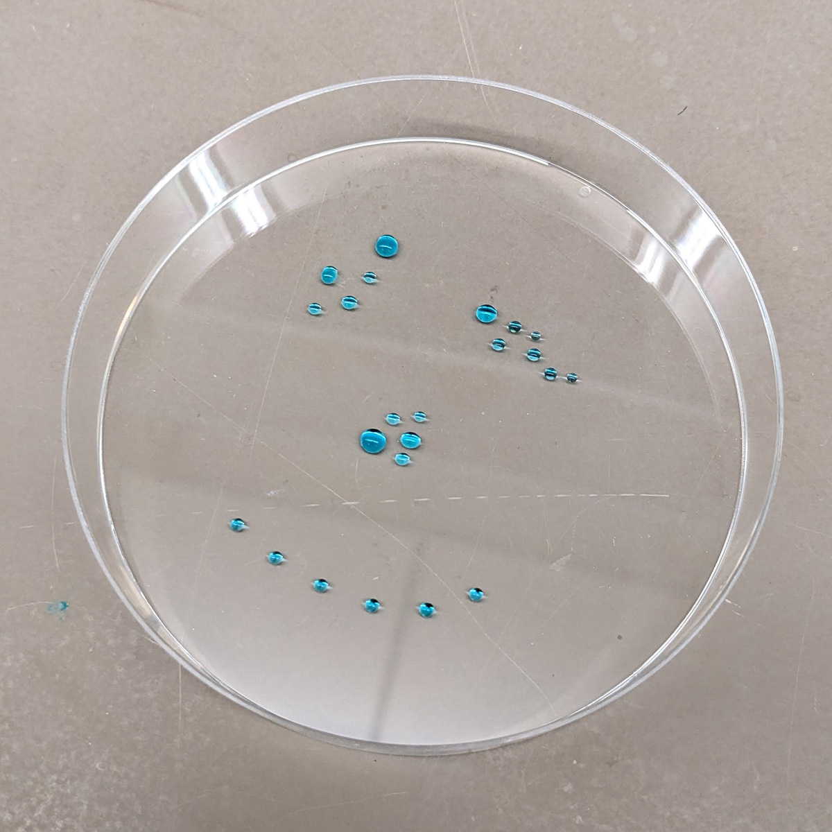
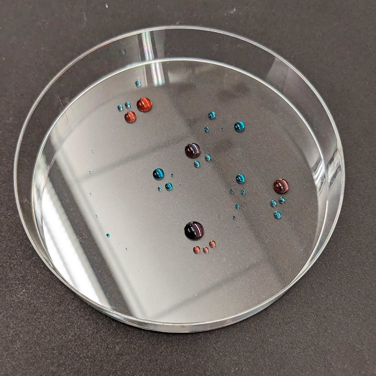
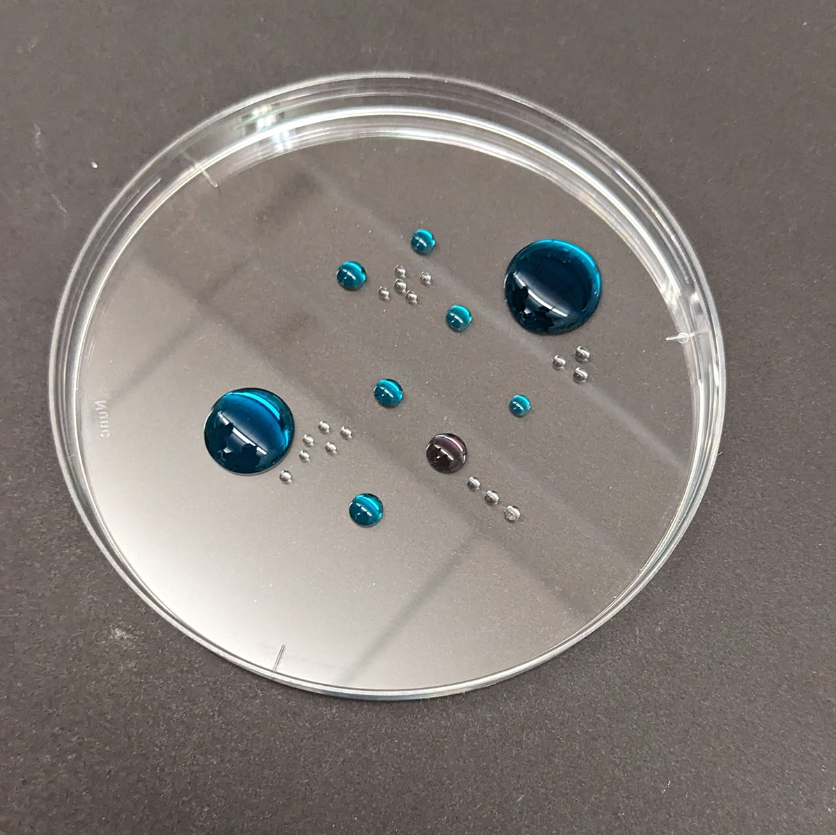
Part C: Planning the Global Experiment | Cell-Free Master Mix Design
sfGFP sfGFP is useful in cell-free systems because it is engineered for robust folding and is also a fast-maturing GFP variant, which helps fluorescence appear quickly and reliably even when expression conditions are not ideal. Like other GFP-like proteins, however, chromophore maturation still depends on oxygen, so fluorescence can lag if oxygen availability is limited.
mRFP1 mRFP1 is a slowly maturing red fluorescent protein, so the protein may be present before the fluorescence is fully visible, which can make short cell-free reactions underestimate expression. It is reported to have relatively low acid sensitivity, which can help preserve signal if the reaction drifts slightly in pH over long incubations.
mKO2 mKO2 is generally valued because it is a relatively fast-maturing orange fluorescent protein, which is helpful when comparing fluorescence over limited reaction times. It also has moderate acid sensitivity, so pH drift in a long cell-free incubation could reduce its apparent brightness.
mTurquoise2 mTurquoise2 is known for its high brightness and photostability, which makes it a strong reporter when repeated imaging or long observation windows are needed. As a GFP-family fluorophore, it still requires oxygen-dependent chromophore maturation, so final fluorescence depends not only on translation but also on post-translational maturation conditions.
mScarlet-I mScarlet-I is especially attractive in cell-free systems because it was engineered for accelerated maturation relative to mScarlet, which helps red signal appear more quickly in practical experiments. This is useful in long but finite reactions such as 20–36 hour incubations, where maturation speed strongly affects how much fluorescence is visible by the endpoint.
Electra2 Electra2 is a newer blue fluorescent protein, so one relevant consideration is that its performance may be more context-dependent and less broadly benchmarked than older standards like sfGFP or mTurquoise2. As with other fluorescent proteins, usable signal still depends on proper folding and chromophore maturation, so suboptimal reaction chemistry could reduce apparent output even if the protein is translated.
Hypothesis for improving fluorescence over a 36-hour incubation
Hypothesis: Increasing the buffering capacity of the cell-free mastermix and carefully re-optimizing magnesium concentration will improve the 36-hour fluorescence endpoint of mKO2, because stronger pH stability should reduce acid-related signal loss while optimized Mg²⁺ should support translation and folding efficiency.
I would therefore test a condition with slightly higher or more stable buffer capacity together with a small Mg²⁺ titration series. The expected effect is that mKO2 would retain more of its fluorescence over long incubation, rather than losing apparent brightness because of pH drift or suboptimal folding conditions.
Week 2: DNA read write edit
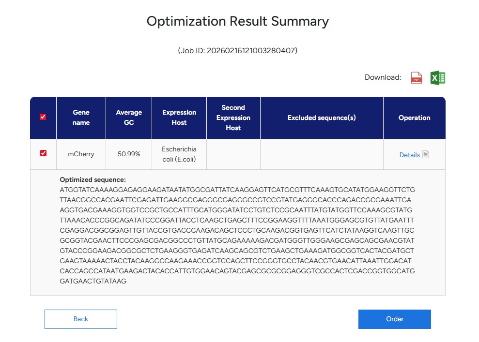
for this week’s HW assignment I’ve chosen the protein mCherry. mCherry is a protein that expresses in red flourescent light emmitance. Fusing it to another protein will enable use to discern wheter the ‘other’ protein is expressed, by visibly observing the red flourescent light. essentially, mCherry functions as a global process visualisation tool across multiple SynBio applications.
Googling mCherry Protein I arrived at the uniprot.org database where I’ve obtained the mCherry sequence:
Using the Gensmart Codon Opt Tool to optimise the above codon seq for E.coli. I chose to opt for E.coli because it is my understanding that this organism serves as a common platform for SynBio uses, and beacuse i’m new to the field, I rather stick to common practices to solidify my understanding when taking first steps in prot-design.
Releying on my understanding of ‘The Central Dogma’, one ’technology’ to produce the protein from the above sequence is the protein creation process that happens inside the Rybozome which is located in a cell’s nucleus. The Rybozome (which is also called R-RNA) is the site that ’takes-in’ M-RNA after it has transcribed a DNA sequence and undergone some editing to the original transcribing. The Rybozome has 2 parts. M-RNA sits in the small part, and gets read by the Rybozome which translates the codons it reads in the M-RNA, and ‘calls’ for T-RNAs to arrive at the big part of the Rybozome. Each T-RNA ‘holds’ and Amino Acid, and when ‘called’ by a respective codon sequence, it arrives at the Rybozome to ‘hand over’ that amino acid. Amino Acids bind to one another in the Rybozome’s bigger part and start forming a chain. This process repeats until the Rybozome ‘finishes’ reading the entire sequence, resulting in a chain of amino acids that will leave the Rybozome and continue to other processes that will eventually result in the aminos folding into a 3D structure that we call a protein.
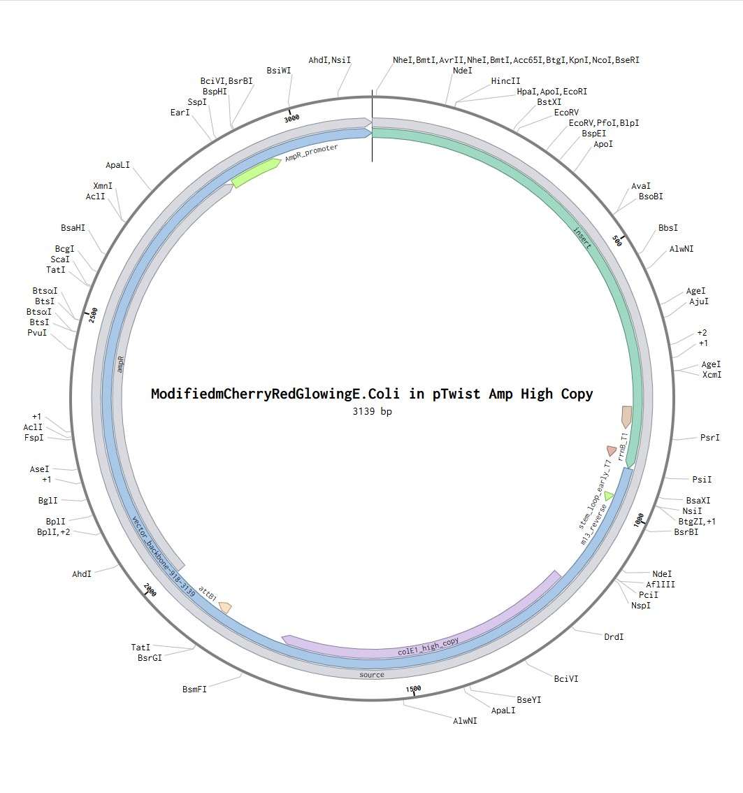
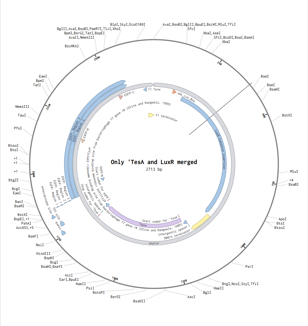
Putting my optimized codon seq into Benchling with the additional sequences provided, I have created a share link to the Benchling file.
Following the steps in the Twist instructions part, I was able to export my Benchling file in .fasta format, upload it to the Twist platform, choose pTwist Amp High Copy Vector and download the .gb file. reuploaded into benchling I can see the resulting expressions cassette! Whohoo (:
What DNA would you want to sequence (e.g., read) and why?
Within the given context, of being introduced to Synbio, I am inclined towards sequencing DNA of organisms and proteins that have something to do with processes of photosynthesis, CO2 sequestration and or flavor and aroma enhancement. The former two have versatile applications in the emerging field of bio-chemical energy production, while the latter have more focused applications in the field of cultivated lab meat, both of them I find highly impactful and worthwhile endeavors to pursue.
In particular, I can propose to read the DNA of the RuBisCO enzyme, that binds a CO2 molecule to a RuBP molecule and creates two 3-carbon molecules. This is a part of the larger photosynthesis process where an organism is converting light energy into sugars and CO2 is being ‘stored’ in sugars. At the same time the photosynthetic process could also be tapped into, converting free electrons created in the process to electrical energy. Enhancing the processes underlying photosynthesis means potentially improving electrical energy yield and carbon sequestration, two much needed capabilities in our time.
In lecture, a variety of sequencing technologies were mentioned. What technology or technologies would you use to perform sequencing on your DNA and why?
For reading RuBisCO genes, from my understanding, I would go for the Sanger reading process. It’s considered high accuracy, and fit for sequences that are on the order of ~700bp.
Is your method first-, second- or third-generation or other? How so?
Sanger is considered a first-gen method due to the fact that it reads the sequence one-by-one. ‘Next-Gen Methods’ tend to read arrays in parallel making them faster and more cost-effective.
What is your input? How do you prepare your input (e.g. fragmentation, adapter ligation, PCR)? List the essential steps.
A Sanger reaction will typically require the reaction-medium, a template DNA (could be a purified PCR or a plasmid), and a primer.
If using a Purified PCR, the primers used for the PCR process would work effectively as primers for the Sanger process as well.
Each primer will read roughly ~700bp so for reading longer sequences you would need to tile primers one after the other. If the sequence is in the right size, you could sequence it in 2 ‘runs’ using a forward reading primer and a reverse reading primer and notice where they overlap.
What are the essential steps of your chosen sequencing technology, how does it decode the bases of your DNA sample (base calling)?
Lets say I am performing the Sanger reaction with a purified PCR. I would take the Sanger mix (the medium in which the Sanger reaction occurs), my purified RuBisCO PCRs, and the primer I used for the PCR creation itself. Based on the size of the PCR (in bp units) I will decide how many primers I need because Sanger reads around ~700bp. Preferably the best results are achieved either with a sequence length that is suitable for a single primer use or dual-primer use, in which case I will utilize both a forward reading primer and a reverse reading primer. ‘base calling’, or identification of ATCG nucleotides is done by attaching a fluorescent ddNTP after bases occasionally. The ddNTP stops the sequence’s extension, serving as a ‘cap’ of sorts. While copying the sequence many times, the RNA polymerase will attach the ddNTP label multiple times, effectively creating many copies of the DNA in all possible lengths. These ddNTP fluorescent caps will serve as a labels that could be seen after the entire batch had been separated by length in an electrophoresis process. A sorting algorithm is then deployed, identifying the different colors and lengths of each sequence that shows up, and translating the colors back to bases. so essentially cutting dna and attaching colored labels to cuts, ordering the cuts by size, translating color + size results back to bases sequence using software.
What is the output of your chosen sequencing technology?
The output of the Sanger process is the chromatogram, a color-coded graph that shows peaks where the respective base had been identified along the length of the sequence, and the base-called sequence that is derived from it.
What DNA would you want to synthesize (e.g., write) and why?
Going back to the first question in this assignment, in the given context, I am inclined towards modifying DNA of organisms and proteins that have something to do with processes of photosynthesis, CO2 sequestration and or flavor and aroma enhancement. The former two have versatile applications in the emerging field of bio-chemical energy production, while the latter have more focused applications in the field of cultivated lab meat, both of them I find highly impactful and worthwhile endeavors to pursue.
In particular, I can propose to write the DNA of the RuBisCO enzyme, enhancing it’s ability to bind CO2 molecules to RuBP molecules more effectively. Enhancing the processes underlying photosynthesis means potentially improving electrical energy yield and carbon sequestration,.
What technology or technologies would you use to perform this DNA synthesis and why? How does your technology of choice edit DNA? What are the essential steps?
I believe that for modifying a DNA sequence I would order oligos of the chosen sequence, perform a fragment replacement on the specific point in the sequence I assume will result in enhancing the desired trait (In my case is improving the ability of RuBisCO enzyme to bind CO2 molecules to RuBP molecule), assemble all fragments together in assembly process (Gibson?), and then sequence the entire dna to verify that I’ve assembled it correctly.
What preparation do you need to do (e.g. design steps) and what is the input (e.g. DNA template, enzymes, plasmids, primers, guides, cells) for the editing?
First I will need to make sure I have the proper assessment tools to determine success or failure. If the RuBisCO enzyme is binding CO2 molecules, it makes sense to creating a testing environment where I could measure rate of of CO2 dissappearance for example. I would then proceed to select sites for the mutation to happen (multiple sites or a specific target site, depending on available prior knowledge.). The next step would be to create primers that target these specific sites and change some bases, or if a larger chain needs to be replaced, I would create entire custome fragments. After that I would assemble the modifyied DNA, Sequence it to make sure I’ve assembled the intended sequence, and test it. Required inputs would include: template palsmids containing a PCR product of RuBisCO or the gene itself, primers or entire fragments for replacing, polymerase for duplicating the sequence, and assembly enzymes to ‘stich’ the new sequence together. If going with a plasmid, I will need the backbone itself, host cells to insert the plasmid to, and a sequencing technology to verify my work (Sanger was mentioned earlier but it depends on the actual planned sequence legnth in bp units)
What are the limitations of your editing methods (if any) in terms of efficiency or precision?
The polymerase process may introduce errors in copying the sequence. This is also true for assembly of large fragments as well, they could introduce unintended changes during assembly, this tends to happen if you try to assemble a bigger fragment count, repetitive fragments, or very long ones.
References:
Adams, J. (2008) DNA sequencing technologies. Nature Education 1(1):193
Published in Synthetic Biology (Volume 8, Issue 1, 2023), the paper presents a new open-source script for the Opentrons OT-2 robot called “AssemblyTron.” The paper overviews automation in the context of synthetic biology’s repeating workflow (the DBTL cycle) and argues that experimental progress is often constrained by the labor and tacit expertise required to carry out repetitive, error-prone bench work. These standards are crucial for reliable experimentation, but the paper suggests automation can help by:
Reducing opportunities for human pipetting error and improving consistency
Lowering the hands-on training burden for repetitive liquid-handling steps
Minimizing time, cost, and waste
The authors describe using AssemblyTron to streamline DNA assembly/cloning workflows on the OT-2, including automating PCR fragment preparation and the setup of multipart DNA assembly reactions from designed DNA parts/fragments. The discussion concludes by emphasizing the potential for lowering barriers and increasing accessibility in synthetic biology experimentation, along with future directions for improving and extending the script.
Write a description about what you intend to do with automation tools for your final project. You may include example pseudocode, Python scripts, 3D printed holders, a plan for how to use Ginkgo Nebula, and more. You may reference this week’s recitation slide deck for lab automation details.
One idea that I could explore with automation regarding the Living Scaffold Final Project I suggested in Week 1 would be automated “parameter sweeps” for mapping purposes. Automation would let me treat the living scaffold as a controllable, testable system: running repeatable parameter sweeps, collecting data, and potentially implementing closed-loop control of light and media conditions to map oxygen distribution. Basically what I’m suggesting here is to run the same experiment across many conditions without human variability, to see how oxygen generation/distribution changes with different inputs:
Different light cycles (intensity, pulsing, duty cycle)
Different media compositions (nutrients, buffering, additives that affect scaffold properties)
Different co-culture ratios (photosynthetic layer density vs scaffold thickness)
Different geometry variants (channels/porosity patterns)
Week 4: Protein Design 1
Part A. Conceptual Questions
How many molecules of amino acids do you take with a piece of 500 grams of meat? (on average an amino acid is ~100 Daltons)
Some definitions regarding measurement units:
A Dalton (Da) is a unit used to describe molecular mass. A useful heuristic is: 1 Da ≈ 1 g/mol
A mole (mol) is a counting unit in chemistry: 1 mol = 6.022 × 10^23 molecules (Avogadro’s number).
If we assume an amino acid (AA) is ~100 Da, this corresponds to ~100 g/mol. Meat is not entirely protein; if we assume protein is ~20% of meat by mass, then 500 g meat ≈ 100 g protein.
100 g ÷ (100 g/mol) = 1 mol ≈ 6.022 × 10^23 AA units.
So, 500 g of meat contains on the order of ~6 × 10^23 amino-acid “units” worth of protein mass, given the assumptions above. (OpenStax, n.d.)
Why do humans eat beef but do not become a cow, eat fish but do not become fish?
When we digest proteins, our body breaks them down into smaller peptides and then into amino acids. Protein breakdown in digestion can be described in three stages:
Stomach: Hydrochloric acid (HCl) lowers pH and helps denature proteins (unfolding them). The enzyme pepsin begins cutting long polypeptides into shorter peptides. (OpenStax, n.d.)
Small intestine: Pancreatic proteases (e.g., trypsin and chymotrypsin) continue cutting peptide bonds into smaller peptides and some free amino acids. (OpenStax, n.d.)
Brush border: Enzymes on the intestinal “brush border” complete digestion into amino acids and very short peptides that can be absorbed into the bloodstream and distributed throughout the body for building human proteins. (OpenStax, n.d.)
Why are there only 20 natural amino acids?
The standard genetic code encodes 20 amino acids, with two rare genetically encoded additions: selenocysteine (including in humans) and pyrrolysine (in some microbes). A key point is that amino acids are not only “letters” for variety; they are the building blocks that enable proteins to reliably fold into stable, soluble, close-packed 3D structures with functional binding pockets. (Doig, 2016)
Evolution likely began with a smaller set of amino acids, then expanded the “vocabulary” as biological complexity increased. However, beyond a certain point, adding new amino acids yields diminishing returns and increases system-level costs: folding stability becomes harder to maintain, translation errors become more costly, and codon assignments become harder to manage without confusion. This challenges the idea that the set is purely a “frozen accident” and supports the view that the 20-amino-acid set is close to an optimal balance between chemical diversity and translational reliability. (Doig, 2016)
Where did amino acids come from before enzymes that make them, and before life started?
This answer splits into two domains: extra-terrestrial and terrestrial sources. Extra-terrestrially, amino acids have been detected in carbon-rich meteorites, suggesting that early Earth could have received a chemically diverse mixture of amino acids from space. (Kirschning, 2022)
Terrestrially, multiple plausible prebiotic routes could generate amino acids through abiotic chemistry in different environments—so it’s unlikely there was a single origin location. Examples include Strecker-type synthesis and Miller–Urey style discharge experiments, as well as hydrothermal and iron–sulfur mineral settings that can promote reaction networks from simple precursors. Wet–dry cycles (e.g., in hydrothermal fields) are important because they can repeatedly concentrate reactants and support peptide formation, bridging from free amino acids toward short peptides. (Kirschning, 2022)
If you make an α-helix using D-amino acids, what handedness (right or left) would you expect?
An α-helix made from D-amino acids is expected to be left-handed (the mirror-image of the common right-handed α-helix formed by L-amino acids). This follows from stereochemistry: switching from L to D reverses the preferred helical handedness. (Doig, 2016)
Can you discover additional helices in proteins?
Yes. Besides the α-helix, proteins can also contain 3_10 helices and π-helices. A 3_10 helix is typically tighter than an α-helix (fewer residues per turn), often appearing as short segments. A π-helix is rarer and is often described as an insertional “bulge” within α-helices that can contribute to function (e.g., shaping binding pockets). (Cooley et al., 2010)
Why are most molecular helices right-handed?
In proteins built from L-amino acids, the right-handed α-helix is strongly favored because it minimizes steric clashes and supports favorable backbone geometry and hydrogen bonding. Left-handed α-helices in L-amino-acid proteins tend to be destabilized by unfavorable backbone/side-chain interactions. (Doig, 2016)
Why do β-sheets tend to aggregate? What is the driving force for β-sheet aggregation?
β-sheets tend to aggregate because exposed β-sheet edges can “zipper” together through backbone hydrogen bonds (edge-to-edge pairing). In water, aggregation is often further stabilized when hydrophobic side chains pack together and exclude water, promoting larger assemblies. (Nowick, 2008)
Why do many amyloid diseases form β-sheets? Can you use amyloid β-sheets as materials?
Many amyloid diseases involve proteins that misfold and assemble into highly stable β-sheet-rich fibrils (amyloid), which can accumulate in tissues and disrupt function. β-sheet structures can expose edges that promote repeated “zippering” and stacking into fibrils, making them unusually stable. (Nowick, 2008)
Because amyloid fibrils can be rigid, chemically stable, and programmable by sequence, they are also being explored as functional biomaterials (with careful design and safety considerations). As one review summarizes: “The rigidity, chemical stability, high aspect ratio, and sequence programmability of amyloid fibrils have made them attractive candidates for functional materials…” (Li & Zhang, 2021)
Part B: Protein Analysis and Visualization
Briefly describe the protein you selected and why you selected it.
Myoglobin is an oxygen-binding protein in muscle that stores and shuttles O₂ inside cells using a heme group, and its oxygen/oxidation state is a major reason meat looks red vs brown. In the cultivated-meat “marbling/structure” project, it’s directly tied to the sensory realism problem: getting cultured tissue to develop the same color cues people associate with meat. It interests me because it links a visible outcome (color) to a real underlying biological variable (oxygen handling and tissue state), which is a legible bioengineering lever I can explore in my final project proposition.
Identify the amino acid sequence of your protein. How long is it? What is the most frequent amino acid?
Downloaded the AA sequence for Myoglobin (one of five variations in humans) from the Uniprot website
it is 154 Amino Acids long, and the most frequent Amino Acid within the sequence is Lysine (coded in the sequence as K), and it appears 20 times in the chain.
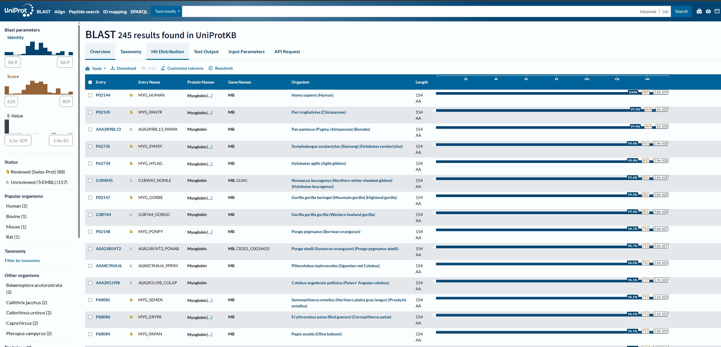
How many protein sequence homologs are there for your protein? Does your protein belongs to any protein family?
Using the Uniprot BLAST tool, I analysied the Myoglobin sequence and found that there are 250 homologs for this protein across the swiss-prot and trEMBL datasets.
looking up Myoglobin I arrived at the Interpro webpage where Myoglobin was identified to be a member of the globin domain (Pfam category PF00042)
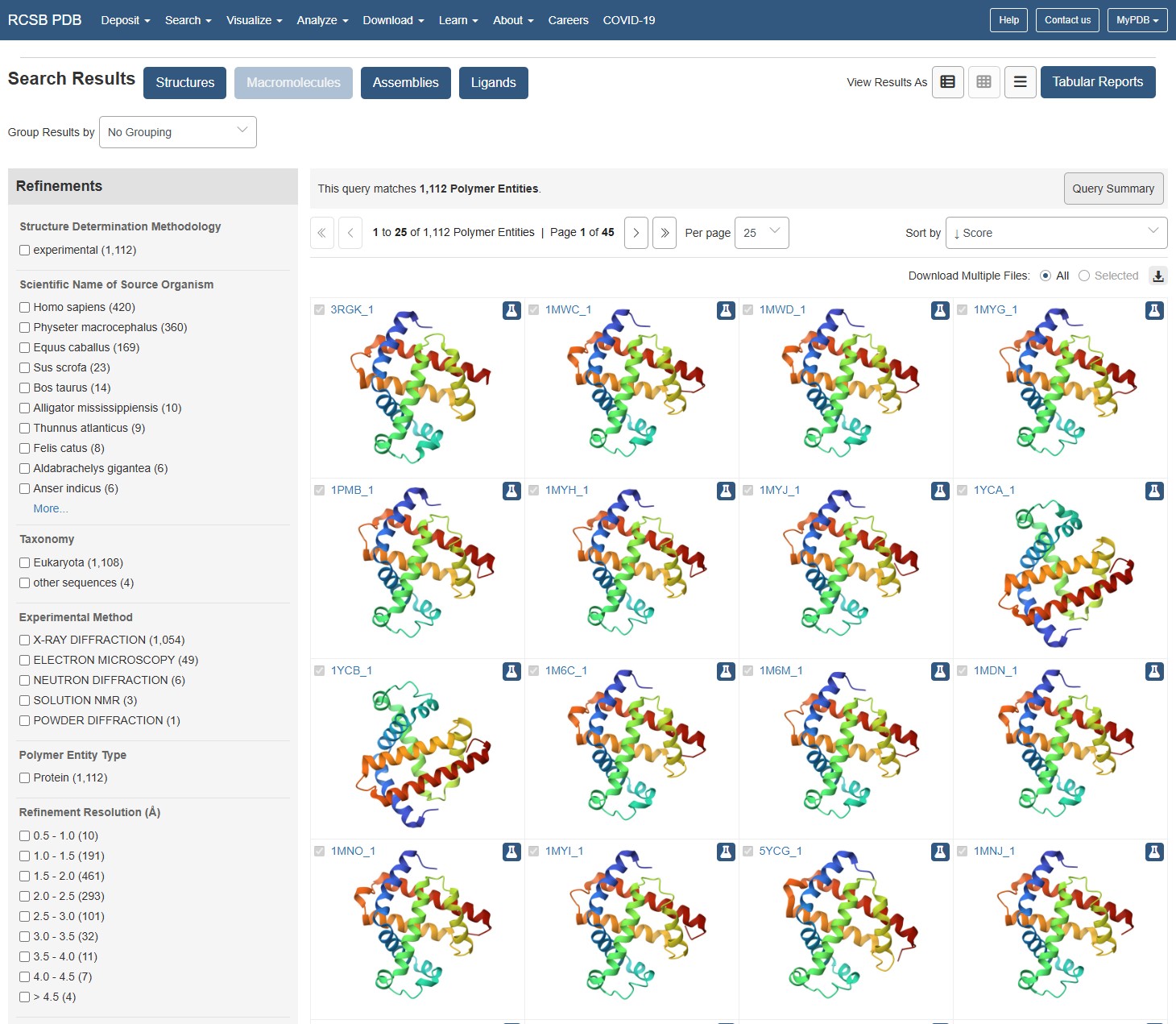
Identify the structure page of your protein in RCSB When was the structure solved? Is it a good quality structure?
using the RCSB website to identify Myoglobin structure, I can see the structure has been documented many times, in increasing resolutions. The earliest documented structure on the website dates to 1975. The best resolutions available (10 entities) are within the 0.1-0.5A range, and these are dated to be between 2005-2024. I would say for the latest entities, they populate the best resolution category available on the webpage so they should be considered as excellent quality.
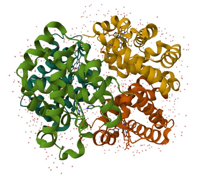
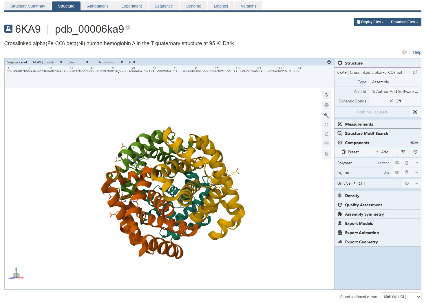
Are there any other molecules in the solved structure apart from protein? Does your protein belong to any structure classification family?
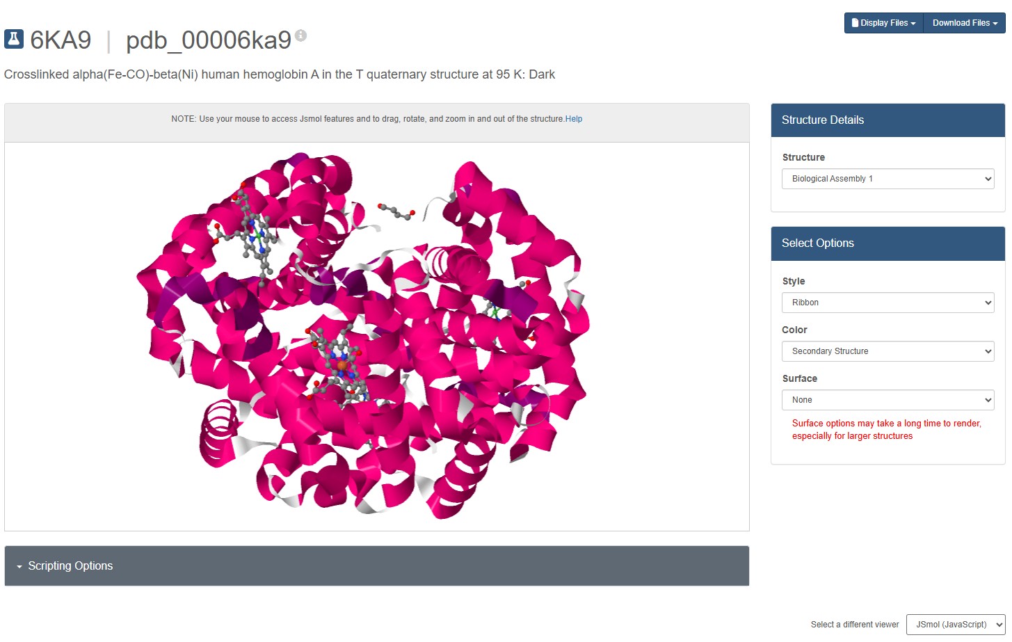
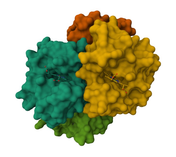
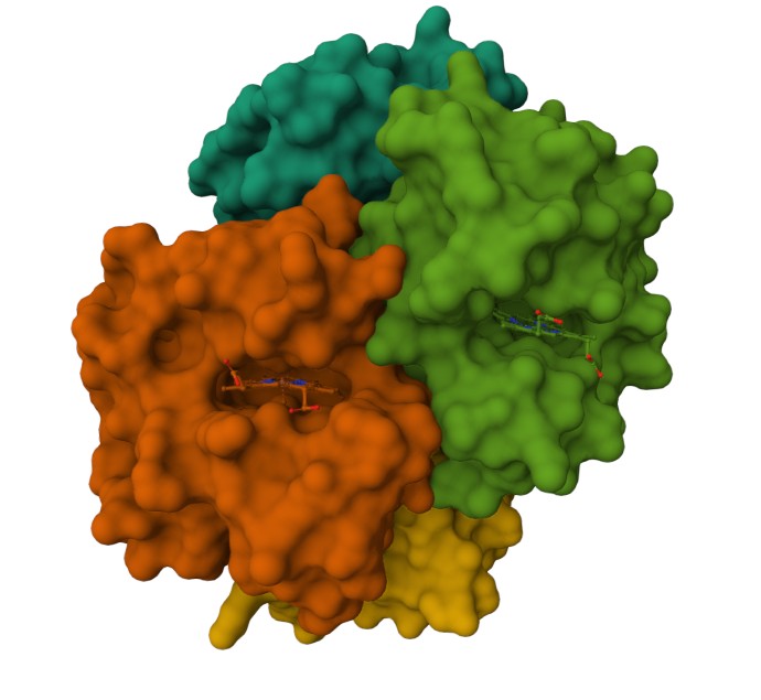
Using the 3D render and data provided for 6KA9 (the first RCSB search result: Crosslinked alpha(Fe-CO)-beta(Ni) human hemoglobin A), I can see there are O molecules scattered across the 3D render. This seems to be due to the protein modeled while being in an aqueos solution. Besides the water, only Polymer and Ligand groups are present in the render, which make the entire protein quaternary structure.
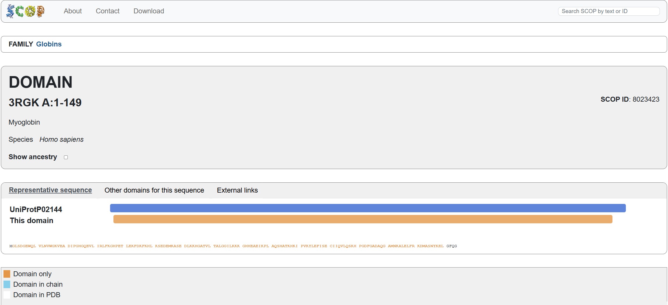
Does your protein belong to any structure classification family?
Using the SCOP tool shows that Myoglobin is a member of the 3RGK A:1-149 domain (SCOP ID 8023423). it also notes that it is a member of the Globins family, which matches the protein family we say Myoglobin associated with in the earlier question.
Visualize the protein as “cartoon”, “ribbon” and “ball and stick”.
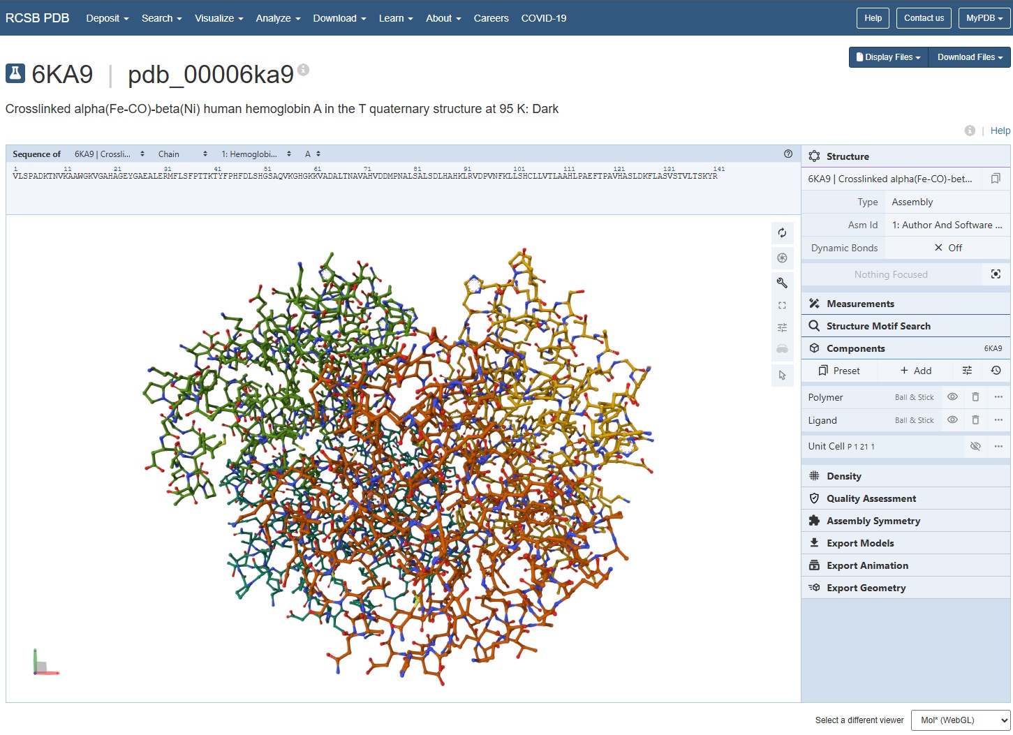
For this assignment, I used the RCSB 3D visualisation webapp that runs Mol* (WebGL) for 3D renderings.
Because the “cartoon” representation for the ligand groups did not show anything, I assigned them a “line” representation so they will be visible.
Mol* does not seems to have a “ribbon” representation. I switch to JSMol in the RCSB 3D Visualisation webapp, and chose a ribbon representation.
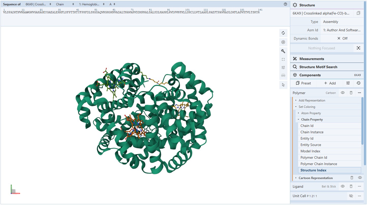
Going back to Mol* (because I think it creates nicer renderings), we get the “ball and stick” representation.
Coloring secondary structures (and honestly we could even determine this before, but to be on the safe side), we can see the Myoglobin protein variant I’m visualising consists only of α-helices as Polymer structures (They are all colored the same).
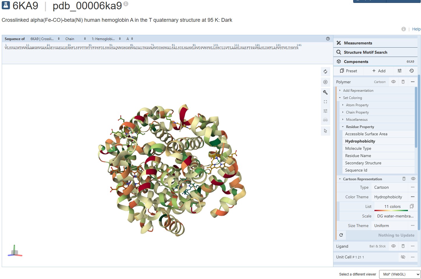
Coloring the protein for hydrophobicity, we discover the molecules vary in their hydrophobic charecteristics, varying across a scale of 11 different degrees. The spread is a bit confusing and I’m not sure I can draw a solid conclusion from it. It seems the protein is mostly hydrophillic, but certain molecules demonstrate a strong hydrophobic attribute.
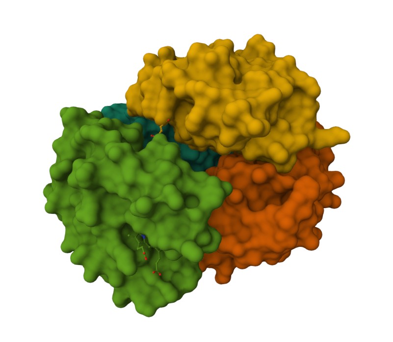
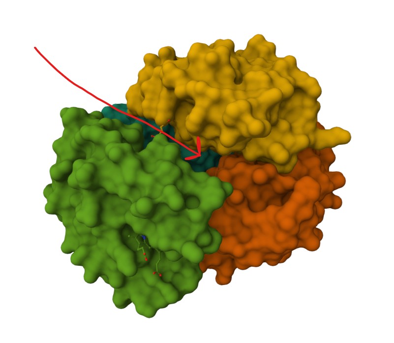
Representing the protein using surfaces, we can immidiatly tell there is a central pocket. Another interesting observation available through the surface render is that the Ligand groups have their own ‘mini pockets’ where they are tucked into the Polymer structure.
Surface representation
Observing the central pocket
Tucked Ligand groups
C1. Protein Language Modeling
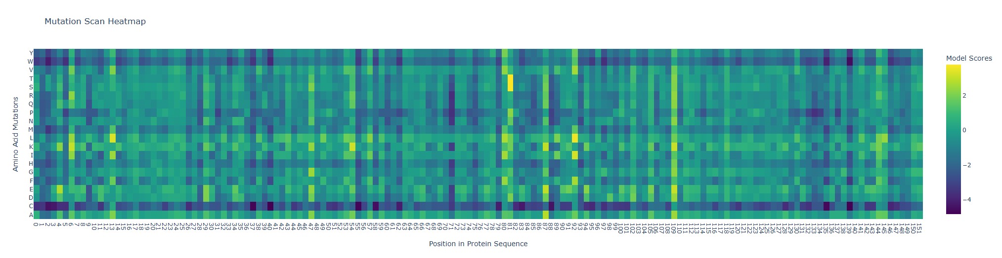
Use ESM2 to generate an unsupervised deep mutational scan of your protein based on language model likelihoods.
Can you explain any particular pattern?
Looking at the heatmap, position 92 (wild-type Q, glutamine) stands out because the substitutions Q→L and Q→I get unusually high model scores (bright yellow). In ESM2 terms, that means the model thinks Leu or Ile “fit” well at that position in a myoglobin-like sequence.
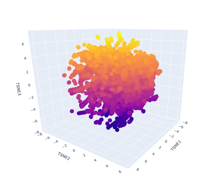
Latent Space Analysis: Use the provided sequence dataset to embed proteins in reduced dimensionality.
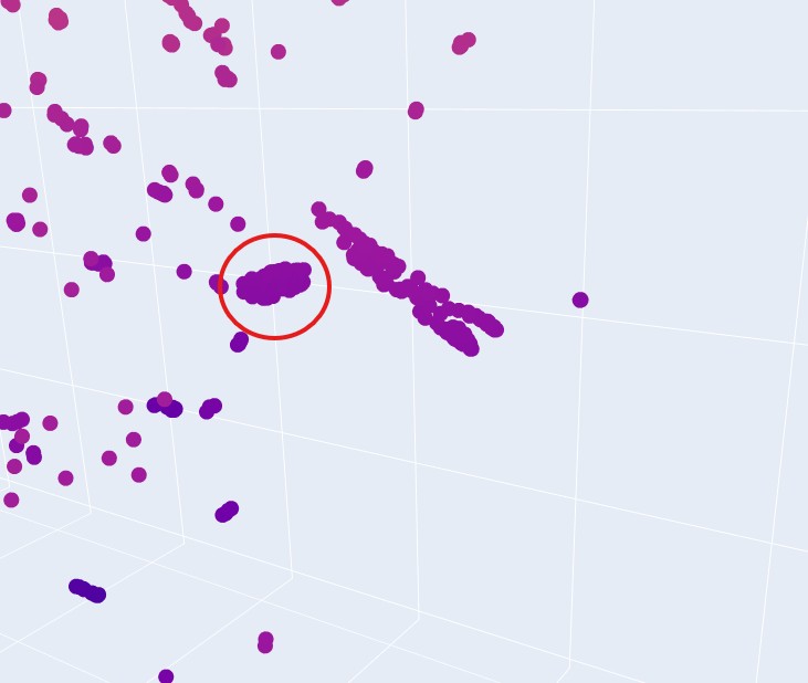
Analyze the different formed neighborhoods: do they approximate similar proteins?
Yes, it seems that when zooming in, specific proteins tend to group in neighbourhoods based on their 3 t-SNE coordinates. like this group:
This implies that they have very similar sequence, domain or group, and therefore can be expected to have similar fold structures. They do not, however share the same taxonomy. That is understood immidiatly when you hover over some group of proteins and see that their taxonomy is varied across multiple species.
References
Cooley, R. B., Arp, D. J., & Karplus, P. A. (2010). Evolutionary origin of a secondary structure: π-helices as cryptic but widespread insertional variations of α-helices enhancing protein functionality. Proceedings of the National Academy of Sciences, 107(25), 11285–11290. https://pmc.ncbi.nlm.nih.gov/articles/PMC2981643/
Li, C., & Zhang, X. (2021). Amyloids as building blocks for macroscopic functional materials: Designs, applications and challenges. International Journal of Molecular Sciences, 22(5), 1–28. https://pmc.ncbi.nlm.nih.gov/articles/PMC8508955/
Changing the 4th residue (In much of the SOD1/ALS literature, that first methionine (M) is considered removed in the mature protein, so residue numbers shift by minus 1.)
wild type: MATKAVCV…
mutant: MATKVVCV…
Running the sequence of the A4V mutated SOD1 in the PepMLM Collab, asking for 4 different peptides at the length of 12 AA’s with K = 5.
I want to note that I do observe X to appear in 3 out of 4 sequences, more specifically the top 2 scoring sequences end with an X. This may be an issue downstream.
Noting that the Alphafold server does not allow to input sequences containing an X AA, I return to the PepMLM notebook to continue generating peptides under the same parameters until I have 4 valid candidates for Alphafold.
It took a couple more iterations but finally I got 4 valid, generated, peptide predictions.
Running the SOD1 V4A mutation alone first in the Alphafold server to get familiar with it’s shape before I model more peptides in the scene.
For clarity, highlighted in pink is the mutated residue (I manually replaced the V residue in the 4th position with an A residue before inputting the sequence to the Alphafold server)
I can also verify this seems to be a good representation of the modeled SOD1 mutated protein using it’s Alignment Residue graph and high pTm score of 0.96.
Below is the provided explantation for the scores from the Alphafold server
How can I interpret confidence metrics to check the accuracy of structures?
pTM and ipTM scores: the predicted template modeling (pTM) score and the interface predicted template modeling (ipTM) score are both derived from a measure called the template modeling (TM) score. This measures the accuracy of the entire structure (Zhang and Skolnick, 2004; Xu and Zhang, 2010). A pTM score above 0.5 means the overall predicted fold for the complex might be similar to the true structure. ipTM measures the accuracy of the predicted relative positions of the subunits within the complex. Values higher than 0.8 represent confident high-quality predictions, while values below 0.6 suggest likely a failed prediction. ipTM values between 0.6 and 0.8 are a gray zone where predictions could be correct or incorrect. TM score is very strict for small structures or short chains, so pTM assigns values less than 0.05 when fewer than 20 tokens are involved; for these cases PAE or pLDDT may be more indicative of prediction quality.
Moving on to model the interactions of the generated peptides from PepMLM with the SOD1 V4A
For the first peptide on our list, the WRYYAAQAAWKE variant, the model shows a proximity to the N-terminus where the mutation sits, and in the illustrated view we can see it is actually binding. According to ipTM and pTM scores, we learn the folded-form prediction has high confidence grade from the model, while the spatial predicition (how these two models actually interact in the simulated space) is very low, making this first simulation unreliable.
For the second peptide, the WLYPYVAVALAA variant, the model shows again there is no binding between the peptide and the SOD1 V4A protein. This time, the model provides a high confidence score for the fold(pTM), but the ipTM scores read as a ‘failed prediction’ (“values below 0.6 suggest likely a failed prediction.”) and results seems even further away from the target site (Residue 4 near the N-Terminuus). to conclude, the peptide does not serve us well.
For the third peptide, the WRVSVVGVVHGG, results look more promising. ipTM and pTM scores both look strong. the Cartoon view shows that the peptide binds to the SOD1 protein, and it does sit relatively closer to the N-terminus. Getting more comforable with the Alphafold UI I saw an option to switch the illustration mode, where it seems to actually bind to the SOD1 (went ahead and updated all the other simulations as well). I’m unsure if this counts as binding ‘on the target site’, as it’s not precisely touching it, but it is very close. another observation worth mentioning is that it seems this interaction has completley changed the SOD1’s spatial configuration. I think this peptide is a good candidate to proceed.
For the fourth peptide the KVNGAYAGRWLE, which also had the worst psuedo-perplexity score from the PepMLM model (27.7), we see a failed ipTM score, making this simulation irrelevant. A strong pTM results gives confidence about the folding structures, noting this is the first generated-peptide to demonstrate a secondary structure of beta sheets when folded. However, the low ipTM score does not allow me to proceed with this one.
Lastly, simulating the reference peptide FLYRWLPSRRGG also yields failed ipTM scores. I find it surprising, as I was expecting the reference peptide to demonstrate the desired behavior to serve as a reference. while this peptide seems to be bind to the protein for the most part, I cannot trust the outcome due to the very low confidence of the model in the spatial predicition between the two elements. Kind of happy to know one of my generated peptides (WRVSVVGVVHGG) seems more promising than the reference one.
Moving onward to the Peptiverse model to analyise the different metrics we care about regarding our generated peptides:
💧 Solubility
🔬 Permeability (Penetrance)
🩸 Hemolysis
👯 Non-Fouling
⏱️ Half-Life
🔗 Binding Affinity (in context of our mutated SOD1-V4A sequence)
📏 Length
⚖️ Molecular Weight
⚡ Net Charge (pH 7.4)
🎯 Isoelectric Point
💦 Hydrophobicity (GRAVY)
Peptide 1 — WRYYAAQAAWKE
AlphaFold3 gives this complex the lowest ipTM (0.17), and structurally the peptide looks mostly extended and only lightly attached, with limited contact against the SOD1 surface. That visually suggests a weak or unstable interface. PeptiVerse agrees: it predicts weak binding (6.13 pKd/pKi). On the therapeutic side it is still attractive in that it is soluble, permeable, and non-hemolytic, but the structural model does not make it look like a strong binder.
Peptide 2 — WLYPYVAVALAA
This one looks much better structurally: the peptide appears to sit along one face of SOD1 with a broader contact patch, and the ipTM of 0.56 is clearly stronger than pep1, pep4, or the reference. PeptiVerse also gives it the best affinity score of the set (7.367, medium binding). It is predicted to be soluble, permeable, and non-hemolytic, so this is the clearest case where the structure and property model are both favorable. The main caution is that it is fairly hydrophobic and not predicted as “non-folding,” but overall it still looks like the best-balanced lead.
Peptide 3 — WRVSVVGVVHGG
Structurally, this is the strongest-looking AlphaFold3 hit: it has the highest ipTM (0.71) and the peptide seems to make a long, continuous interface across the protein surface, which is exactly the kind of pose you would hope for in a binder. But PeptiVerse does not rank it as the best binder; it is still only weak binding (6.653) and is also predicted to be non-permeable. So this is the clearest mismatch between the two models: best structural interface confidence, but not best therapeutic profile.
Peptide 4 — KVNGAYAGRWLE
This complex is intermediate-to-weak by structure: ipTM is 0.43, and the peptide looks more like a surface appendage on one side rather than a strongly buried binder. PeptiVerse is consistent with that and predicts weak binding (6.095). It is still soluble and non-hemolytic, but also non-permeable, so there is not a strong reason to prioritize it over pep2 or even pep3.
Reference peptide — FLYRWLPSRRGG
The reference peptide gives a low ipTM (0.32) and looks only partially engaged, with the chain remaining fairly extended and not deeply wrapped into the SOD1 surface. PeptiVerse also predicts weak binding (5.968), the weakest of the five by affinity score. Its upside is that it is soluble, highly permeable, non-hemolytic, and the only one predicted as non-folding, which is a nice therapeutic feature, but its binding looks less compelling than the better generated candidates.
Across the whole set, higher ipTM does not map perfectly onto stronger predicted affinity. The clearest example is peptide 3, which has the highest ipTM and pTM scores (which made me favor it moving onward earlier) but only weak predicted affinity, while peptide 2 has the best PeptiVerse affinity despite a lower ipTM than pep3. Also, none of the stronger candidates are predicted to be hemolytic or poorly soluble; all five are predicted soluble and non-hemolytic. The best overall balance of predicted binding plus therapeutic properties is peptide 2 (WLYPYVAVALAA).
I would choose peptide 2 because it gives the best combined picture across both models: the strongest predicted affinity in PeptiVerse, a reasonably strong AlphaFold3 interface (ipTM 0.56), and the model indicates signals of being soluble, permeable, and non-hemolytic.
In the next step we are tasken with running the moPPIt model on the google collab notebook provided. Following instructions I inputted all required data points. However, the final step of retreiveing a csv file with the scored results failed. I tried to change the Runtime modes to CPU, and V5E-1 TPU mode, (originally ran it on the T4 GPU) both have also failed. error code reads “RuntimeError: moo.py failed with code 2”.
Week 6: Genetic Circuits
Week 6 Homework: Genetic Circuits
1. What are some components in the Phusion High-Fidelity PCR Master Mix and what is their purpose?
Phusion High-Fidelity PCR Master Mix contains several key components required for accurate DNA amplification. One central component is the Phusion DNA polymerase, a high-fidelity enzyme with proofreading activity that synthesizes new DNA strands and reduces the error rate compared to standard Taq polymerase. The mix also contains dNTPs (deoxynucleotide triphosphates), which serve as the molecular building blocks used to construct the new DNA strand during amplification.
Another important component is the reaction buffer, which maintains the correct chemical environment for the polymerase to function efficiently. This buffer includes salts and magnesium ions (Mg²⁺), which are essential cofactors for polymerase activity and influence primer binding and enzyme performance. The mix may also include stabilizing agents that help preserve enzyme activity during thermal cycling. Because it is provided as a master mix, many of these ingredients are already pre-balanced, which reduces pipetting error and improves consistency across reactions.
2. What are some factors that determine primer annealing temperature during PCR?
Primer annealing temperature during PCR is determined primarily by the melting temperature (Tm) of the primers. The Tm depends on several sequence features, especially primer length, GC content, and base composition, since G–C pairs form three hydrogen bonds and are therefore more thermally stable than A–T pairs. Primers with higher GC content or longer length typically have a higher Tm and therefore require a higher annealing temperature.
A second factor is the degree of complementarity between the primer and the target sequence. If the primer sequence has mismatches with the target, annealing may be weaker and require optimization at a lower temperature, though this may reduce specificity. The salt concentration and reaction conditions in the PCR mix also affect hybridization behavior, because ionic conditions influence DNA duplex stability. In practice, the annealing temperature is usually chosen a few degrees below the primer Tm in order to balance efficient binding with high specificity.
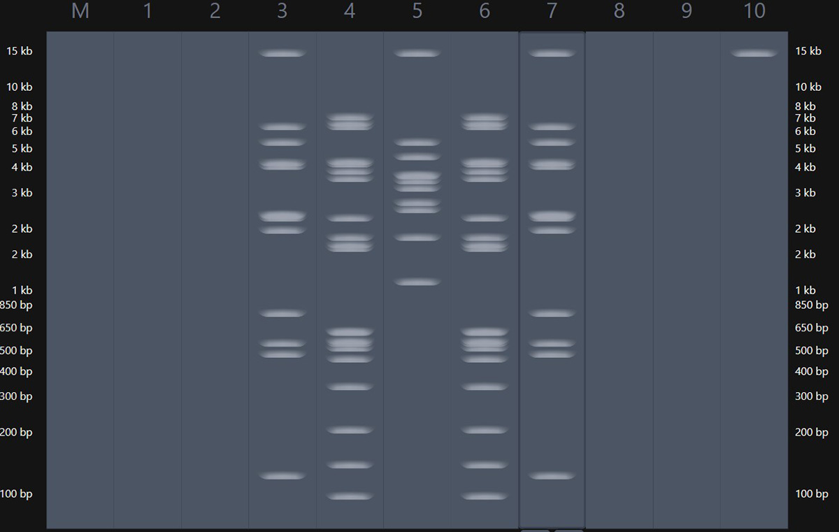
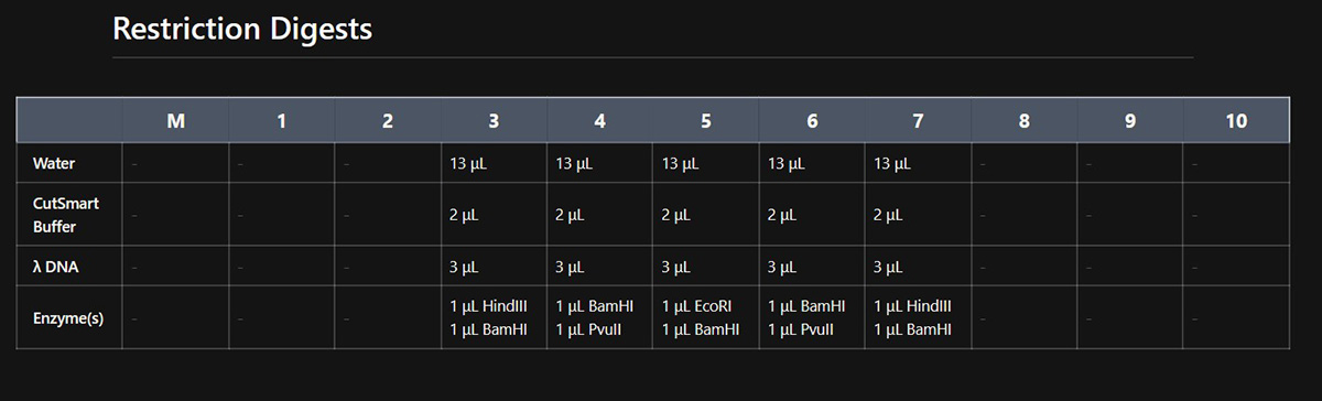
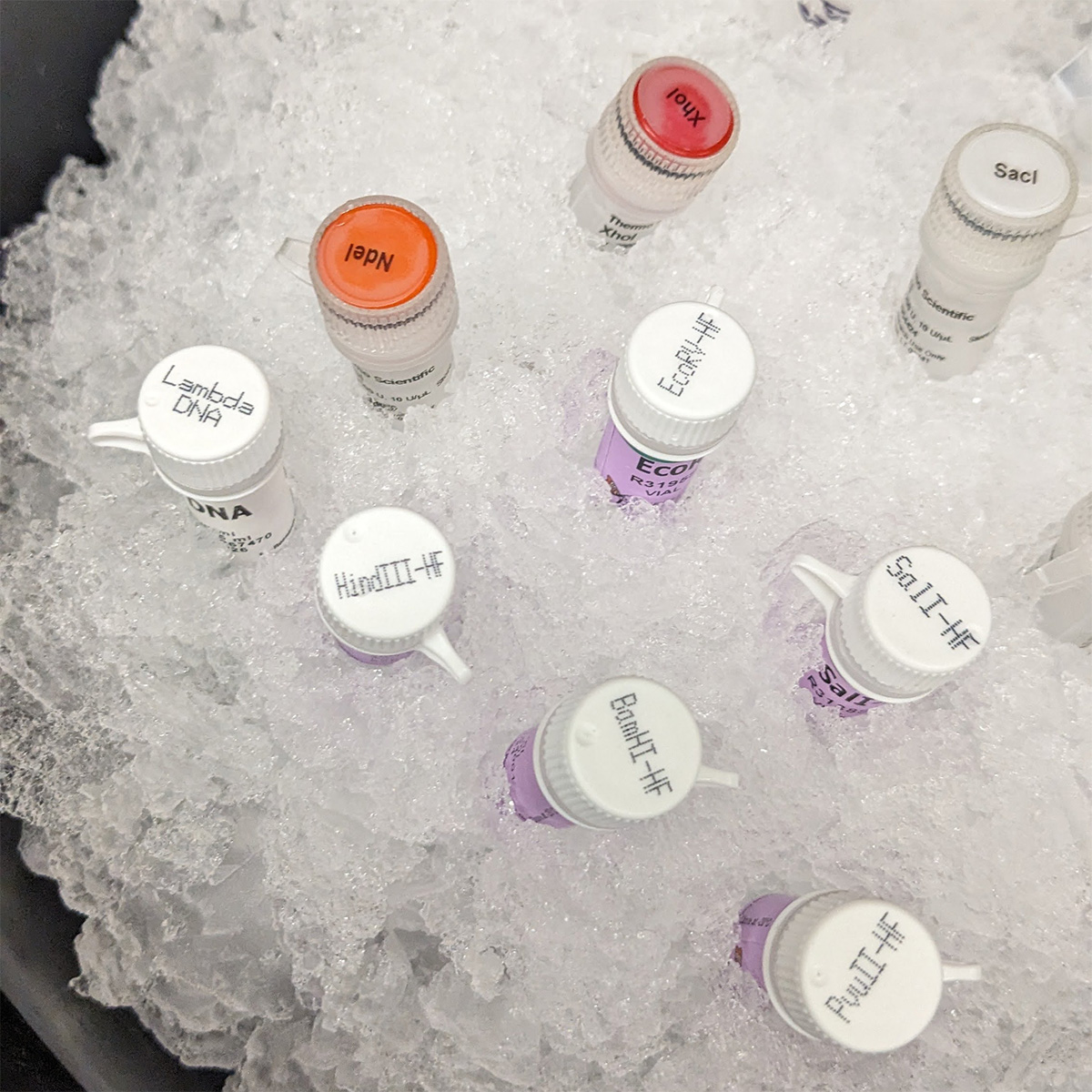
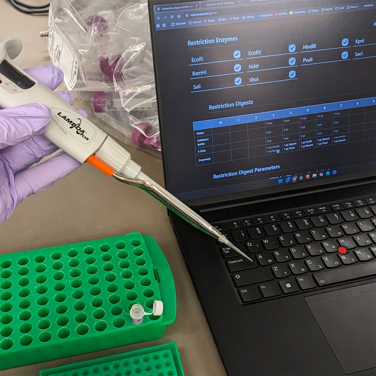
3. There are two methods from this class that create linear fragments of DNA: PCR, and restriction enzyme digests. Compare and contrast these two methods, both in terms of protocol as well as when one may be preferable to use over the other.
PCR and restriction enzyme digestion can both generate linear DNA fragments, but they do so through very different mechanisms. PCR creates a linear fragment by enzymatically amplifying a specific region of DNA using primers, polymerase, dNTPs, and thermal cycling. The protocol involves repeated cycles of denaturation, primer annealing, and extension, which selectively amplify the region bounded by the primer pair. PCR is especially useful when a fragment must be isolated precisely, modified through primer design, or generated from a small starting amount of template DNA.
By contrast, a restriction enzyme digest generates linear DNA by cutting an existing DNA molecule at specific recognition sequences. The protocol is generally simpler: plasmid or DNA template is mixed with one or more restriction enzymes, appropriate buffer, and water, then incubated at the temperature optimal for enzyme activity. Restriction digestion is often preferable when the desired fragment is already flanked by known restriction sites and does not require amplification or sequence redesign. It is also useful for opening plasmids or excising inserts when convenient restriction sites are available.
PCR is more flexible because primer design allows the user to define fragment boundaries and add overlaps or other sequence features. However, it can introduce amplification errors or nonspecific bands if poorly optimized. Restriction digests are often cleaner and simpler when the sequence already contains the required cut sites, but they are limited by the availability and placement of those sites. In practice, PCR is often preferred when custom design flexibility is needed, whereas restriction digestion is preferred when a pre-existing construct already contains a convenient cloning architecture.
4. How can you ensure that the DNA sequences that you have digested and PCR-ed will be appropriate for Gibson cloning?
To ensure that digested and PCR-generated DNA fragments are appropriate for Gibson cloning, the most important requirement is that adjacent fragments contain overlapping homologous ends, typically around 20–40 base pairs long. These overlaps allow the Gibson Assembly enzymes to join fragments in the correct order. When PCR is used, these overlaps are usually added directly through primer design. When restriction digestion is involved, the resulting fragment must still be checked to make sure it contains the correct overlap regions relative to the other assembly partners.
It is also important to confirm that the fragments correspond to the intended sequence and orientation. This can be checked computationally by mapping the PCR primers and restriction enzyme cut sites in sequence software such as Benchling. In addition, the fragments should ideally be clean and specific, meaning the PCR gives a single product of the expected size and the digest yields the correct linearized or excised band. Gel electrophoresis and gel extraction are commonly used to confirm fragment size and purify the correct product before assembly.
A final precaution is to verify that the fragment ends do not include unwanted features that would interfere with assembly, such as incorrect overlaps, missing bases, or incompatible sequence order. In short, appropriate Gibson-ready fragments are confirmed by sequence design, overlap design, size verification, and purification before the actual assembly reaction is performed.
5. How does the plasmid DNA enter the E. coli cells during transformation?
During transformation, plasmid DNA enters E. coli cells after the cells have been made competent, meaning temporarily capable of taking up external DNA. In a standard chemical transformation protocol, the cells are treated with salts such as calcium chloride, which helps neutralize the negative charges on both the DNA and the bacterial cell membrane. This reduces electrostatic repulsion and allows the plasmid DNA to associate more closely with the cell surface.
A brief heat shock then creates a transient physical imbalance across the membrane, which helps drive the plasmid DNA into the cell. The exact molecular mechanism is still described somewhat operationally rather than as a single perfectly resolved pathway, but the key idea is that heat shock temporarily increases membrane permeability and promotes uptake of the plasmid. In electroporation, a different method, a short electrical pulse creates temporary pores in the membrane through which DNA can enter.
Once inside the cell, the plasmid is maintained and replicated if it contains an origin of replication compatible with the host. Cells that successfully took up the plasmid can then be selected on antibiotic plates if the plasmid also carries an antibiotic resistance marker.
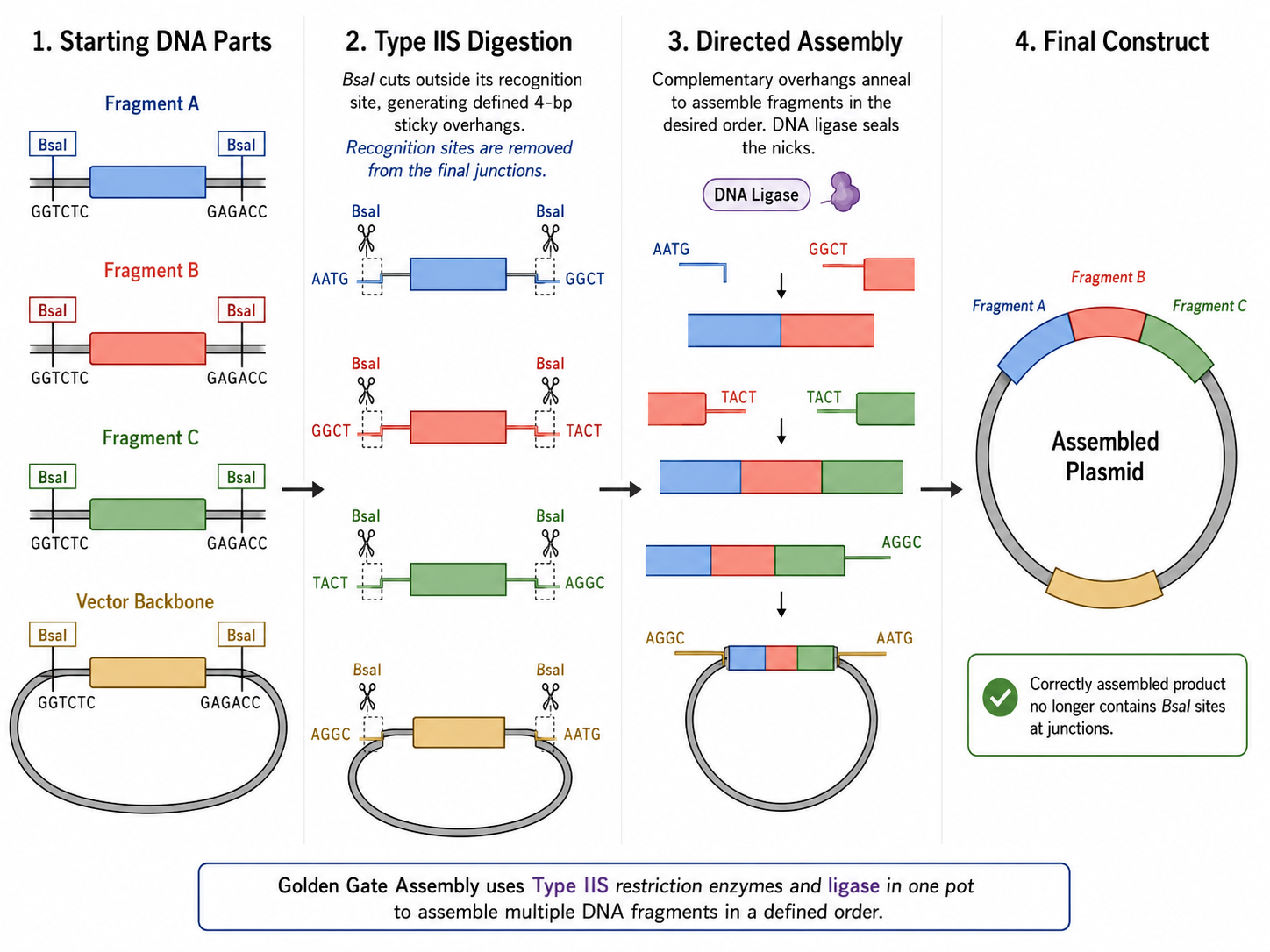
6. Describe another assembly method in detail (such as Golden Gate Assembly)
Golden Gate Assembly is a DNA assembly method that uses Type IIS restriction enzymes together with DNA ligase to join multiple DNA fragments in a defined order within a single reaction. Unlike standard restriction enzymes, Type IIS enzymes such as BsaI cut outside of their recognition sequence, which allows the user to design custom 4-base overhangs on each fragment. These overhangs determine exactly which fragments ligate to each other, enabling seamless and directional assembly without leaving unwanted restriction-site scars between parts. In practice, the DNA fragments and destination vector are designed so that digestion creates complementary overhangs, and the reaction is cycled between temperatures that favor digestion and ligation. Because correctly assembled products no longer contain the original Type IIS recognition sites, they are not re-cut, which enriches the desired final construct over time. Golden Gate Assembly is especially useful for modular cloning, multi-part assemblies, and workflows where many parts must be assembled rapidly and in a predefined order. It is often preferable when standardized part architecture is available, whereas Gibson Assembly may be more flexible when custom overlaps are easier to design than restriction-site-based overhangs.
Week 7: Genetic Circuits 2
Assignment Part 1: Intracellular Artificial Neural Networks (IANNs)
What advantages do IANNs have over traditional genetic circuits, whose input/output behaviors are Boolean functions?
The main advvantage I see of an IANN over a traditional genetic circuit (Boolean in nature) is that the IANN seems better suited for biological situations that require a more sophisticated estimation than a sharp TRUE/FALSE. We would need more ‘sensitive tools’ if we are to deal with many inputs, gradients, dynamic thresholds and intermidiate states - for all mentioned, binary logic is insufficient. I’m interested in cultivated meat, and in this course I will try to demonstrate control over marbeling of fat and meat tissues. This concept matters here because fat distribution is not a binary problem but a morphogentic spatial multi-input issue. IANN’s can seem more relevant when the goal is to account for several factors and generate a site-specific nuanced output.
Describe a useful application for an IANN; include a detailed description of input/output behavior, as well as any limitations an IANN might face to achieve your goal.
A useful application for an IANN, in the context of my meat-fat marbling catalogue direction, would be a system that helps decide where cells in a growing tissue should become more fat-like, more muscle-like, or remain in an intermediate state based on several inputs at once. The inputs could include things like oxygen level, nutrient availability, local signaling molecules, and maybe cell density or position within the scaffold, and the output would be a graded patterning decision rather than a single differentiation switch. What interests me is that this could eventually help produce different marbling motifs or classes instead of just maximizing fat everywhere. A limitation, though, is that a system like this would probably be very sensitive to diffusion, timing, signal decay, and spatial arrangement, so even if the logic works conceptually, getting a stable and precise pattern in real tissue would be difficult. Some of the papers I’ve been reading make that feel plausible as a direction, but also make clear how quickly these systems become messy once spatial biology is involved.
Draw a diagram for an intracellular multilayer perceptron where layer 1 outputs an endoribonuclease that regulates a fluorescent protein output in layer 2.
Assignment Part 2: Fungal Materials
What are some examples of existing fungal materials and what are they used for? What are their advantages and disadvantages over traditional counterparts?
One example of an existing fungal material is mycelium-based packaging or building material, where the fungal network grows through agricultural waste and binds it into a lightweight solid. I find that interesting because it can replace things like foam packaging or some synthetic insulation materials while using low-value waste as feedstock. The main advantages are that it is more biodegradable, potentially lower-emission, and can be grown rather than heavily manufactured. At the same time, the disadvantages are that it is usually less standardized and sometimes less strong, water-resistant, or durable than conventional materials, so it can be harder to use in situations where reliability and repeatability matter a lot.
What might you want to genetically engineer fungi to do and why? What are the advantages of doing synthetic biology in fungi as opposed to bacteria?
If I were engineering fungi, I would be interested in improving the mechanical properties of fungal materials, for example making them stronger or more consistent so they become more useful as design or construction materials. That feels meaningful to me because a lot of the promise of mycelium materials depends not just on being sustainable, but on actually performing well enough to compete with existing options. An advantage of working in fungi instead of bacteria is that fungi already naturally grow as large material-forming networks, so they are better suited for building structural biomaterials rather than just producing molecules in liquid culture. The downside is that fungi are usually slower and more complex to engineer than bacteria, but for material applications they may still be the more relevant organism.
References:
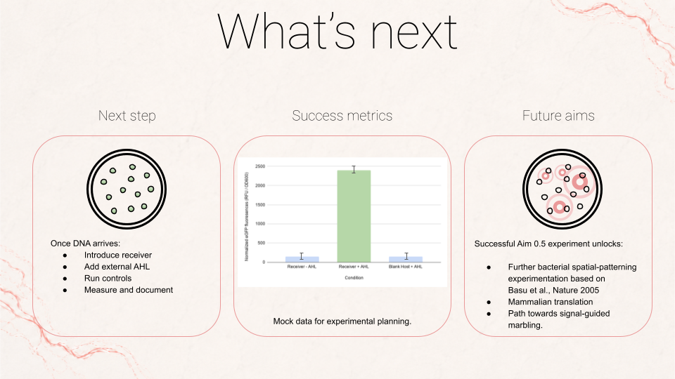
Basu, S., Gerchman, Y., Collins, C. H., Arnold, F. H., & Weiss, R. (2005). A synthetic multicellular system for programmed pattern formation. Nature, 434(7037), 1130–1134.
Mordvintsev, A., Randazzo, E., Niklasson, E., & Levin, M. (2020, February 11). Growing neural cellular automata. Distill, 5(2), e23. https://distill.pub/2020/growing-ca/
Vasle, A. H., & Moškon, M. (2024). Synthetic biological neural networks: From current implementations to future perspectives. BioSystems, 245, 105164. https://doi.org/10.1016/j.biosystems.2024.105164
Week 9: Cell-Free Systems
Cell-Free Systems Homework
1. Explain the main advantages of cell-free protein synthesis over traditional in vivo methods, specifically in terms of flexibility and control over experimental variables. Name at least two cases where cell-free expression is more beneficial than cell production.
Cell-free protein synthesis (CFPS) offers major advantages over traditional in vivo expression because it removes the constraints imposed by maintaining living cells. Since the reaction occurs in vitro, the experimenter has much tighter control over variables such as DNA concentration, energy source, salts, cofactors, reaction timing, and additives. This makes CFPS especially useful for rapid prototyping, because gene circuits or expression constructs can be tested directly without cloning into cells and waiting for growth. It is also easier to study toxic proteins or unstable pathways in CFPS, since there is no living host whose growth is harmed by the product. In addition, freeze-dried cell-free systems are portable, low-maintenance, and can be deployed with minimal equipment, making them well suited for low-resource settings and space applications. This was demonstrated in the BioBits study aboard the ISS, where freeze-dried cell-free reactions were rehydrated and used to express aptamers and fluorescent proteins under microgravity conditions.
Two cases where cell-free expression is more beneficial than cell production are:
Point-of-need biosensing or diagnostics, where portability and rapid response are more important than long-term cell growth.
Expression of toxic or burdensome proteins, where the product would damage or slow the growth of living cells.
2. Describe the main components of a cell-free expression system and explain the role of each component.
A cell-free expression system contains the molecular machinery needed for transcription and translation outside of living cells. One major component is the cell extract, which provides ribosomes, tRNAs, translation factors, metabolic enzymes, and in some cases RNA polymerase. Another component is the DNA template, which encodes the gene or circuit to be expressed. The system also includes nucleotides for transcription, amino acids for translation, and salts/cofactors such as magnesium and potassium that support enzyme activity and ribosome function.
A critical part of the mixture is the energy system, which regenerates ATP and other high-energy molecules needed to power transcription and translation. Many systems also include supplements such as folinic acid, tRNA mixtures, cofactors, and reducing agents to improve expression efficiency. In the BioBits ISS paper, the reaction mixture included ATP, GTP/UTP/CTP, amino acids, potassium glutamate, ammonium glutamate, magnesium glutamate, NAD, CoA, spermidine, putrescine, phosphoenolpyruvate, and cell extract, all of which helped support robust gene expression in vitro.
3. Why is energy provision/regeneration critical in cell-free systems? Describe a method you could use to ensure continuous ATP supply in your cell-free experiment.
Energy regeneration is critical in cell-free systems because transcription and translation consume large amounts of ATP and GTP. Unlike living cells, CFPS reactions do not have intact metabolism to continuously replenish these molecules, so without an energy-regeneration strategy the reaction would stop quickly. Sustained protein synthesis therefore depends on including a substrate that can support ATP regeneration over time.
One common method is to include phosphoenolpyruvate (PEP) as an energy source. In crude extract systems, endogenous enzymes can use PEP to regenerate ATP and maintain the reaction for longer periods. The BioBits formulation used aboard the ISS included 33 mM phosphoenolpyruvate, showing exactly this kind of strategy for sustaining cell-free transcription and translation. In my own experiment, I could use a PEP-based energy system and compare protein yield over time to confirm that the reaction remains active.
4. Compare prokaryotic versus eukaryotic cell-free expression systems. Choose a protein to produce in each system and explain why.
A prokaryotic cell-free system is usually faster, cheaper, and easier to optimize than a eukaryotic system. It is well suited for expressing bacterial proteins, fluorescent reporters, enzymes, or genetic circuits that do not require complex post-translational modifications. For example, eGFP is a good protein to produce in a prokaryotic CFPS system because it folds relatively well, is easy to detect, and does not require glycosylation or other advanced processing.
A eukaryotic cell-free system is better for proteins that depend on more complex folding environments or post-translational modifications such as disulfide bonding, glycosylation, or membrane insertion. For example, a human cytokine or secreted antibody fragment would be a better candidate for a eukaryotic system, because bacterial extracts often cannot reproduce the same maturation steps needed for proper activity. In short, prokaryotic systems are excellent for speed and simplicity, while eukaryotic systems are preferable when the target protein requires more biologically complex processing.
5. How would you design a cell-free experiment to optimize the expression of a membrane protein? Discuss the challenges and how you would address them in your setup.
Membrane proteins are difficult to express in cell-free systems because they tend to misfold, aggregate, or precipitate when no membrane-like environment is available. To optimize expression, I would design a screen in which the same membrane-protein DNA template is tested across multiple reaction conditions that vary membrane mimics, detergent concentration, magnesium concentration, and temperature. A key addition would be some form of membrane support, such as liposomes, nanodiscs, or mild detergents, so that the newly synthesized protein has a hydrophobic environment into which it can insert.
I would also monitor both total expression and soluble/functional expression, since a high total yield is not useful if the protein is aggregated. Suitable readouts might include SDS-PAGE, fluorescence tagging, or an activity assay if the membrane protein has measurable function. A lower reaction temperature and codon-optimized DNA could also help improve folding. Overall, the main challenge is not just producing the protein, but producing it in a membrane-compatible state that preserves structure and activity.
6. Imagine you observe a low yield of your target protein in a cell-free system. Describe three possible reasons for this and suggest a troubleshooting strategy for each.
One possible reason is that the DNA template concentration or quality is poor. If the template is degraded, contaminated, or present at too low a concentration, transcription may be inefficient. A troubleshooting strategy would be to verify the DNA on a gel, re-purify it, and test a range of template concentrations.
A second possible reason is that the reaction chemistry is suboptimal, for example incorrect magnesium concentration, depleted energy source, or poor buffer balance. Since CFPS is very sensitive to reaction composition, I would troubleshoot by running a small matrix of conditions and adjusting magnesium, potassium, and energy-substrate levels systematically.
A third possible reason is that the target protein itself is difficult to express or fold. This is especially likely for large, toxic, disulfide-rich, or membrane proteins. In that case, I would try lowering the temperature, changing the reaction time, adding chaperones or membrane mimics, or switching to a different cell-free system better suited to the protein class.
Homework Question from Kate Adamala
Design an example of a useful synthetic minimal cell
Pick a function and describe it.
My synthetic minimal cell would function as a localized ammonia detoxification sensor-actuator for aquatic environments. Its purpose would be to detect elevated ammonia in contaminated water and respond by producing an enzyme-based output that helps convert ammonia into a less harmful form.
What would your synthetic cell do? What is the input and what is the output?
The input would be elevated environmental ammonia. The output would be expression of a reporter such as GFP together with an enzymatic detoxification module, for example glutamine synthetase activity coupled to ATP-dependent ammonia assimilation.
Could this function be realized by cell-free Tx/Tl alone, without encapsulation?
Not as effectively. Without encapsulation, the reaction would simply mix into the surrounding environment and lose the separation between sensing, response, and controlled release. Encapsulation makes the system behave more like an artificial cell rather than just a biochemical mixture.
Could this function be realized by genetically modified natural cell?
Yes, it could, but that would introduce issues of survival, biocontainment, ecological competition, and environmental release. A synthetic minimal cell would reduce those concerns by remaining non-living and function-limited.
Describe the desired outcome of your synthetic cell operation.
In the presence of elevated ammonia, the synthetic cell should produce a measurable fluorescent signal and activate a detoxification pathway, demonstrating both environmental sensing and a functional biochemical response.
Design all components that would need to be part of your synthetic cell.
The system would need:
a lipid vesicle membrane
a cell-free transcription/translation system
an ammonia-responsive genetic control element
a reporter gene such as GFP
an output enzyme system relevant to ammonia capture or conversion
ATP and metabolic cofactors
permeable access for ammonia or a transport mechanism if needed
What would the membrane be made of?
The membrane could be made of POPC + cholesterol, similar to common synthetic-cell vesicle formulations, because this provides a reasonably stable phospholipid bilayer.
What would you encapsulate inside? Enzymes, small molecules.
Inside I would encapsulate:
bacterial cell-free Tx/Tl extract
amino acids, nucleotides, salts, and energy mix
ATP-regeneration substrate
plasmid DNA for the reporter and detoxification module
glutamine synthetase or related enzymatic module if not produced in situ
Which organism would your Tx/Tl system come from?
A bacterial system would likely be sufficient, because the sensing and output logic do not require mammalian transcription factors or mammalian-specific signaling pathways. A bacterial extract would also be simpler and cheaper.
How will your synthetic cell communicate with the environment?
Ammonia is a small molecule and can cross membranes to some extent, so the input may not require a dedicated channel. If permeability is insufficient, I could incorporate a membrane pore such as alpha-hemolysin (aHL) to facilitate exchange.
Experimental details
Lipids: POPC, cholesterol Genes: GFP reporter, alpha-hemolysin (aHL) if needed for permeability, and a detoxification-related gene such as glnA (glutamine synthetase) How will you measure function? I would measure:
GFP fluorescence as the sensing readout
ammonia concentration before and after treatment as the functional output
optionally, vesicle integrity by microscopy or dye retention
Homework Question from Peter Nguyen
Write a one-sentence summary pitch sentence describing your concept.
I propose a freeze-dried cell-free textile patch that activates on contact with sweat and reports dehydration-related electrolyte imbalance through a visible fluorescent color change.
How will the idea work, in more detail?
The concept is a wearable textile patch containing freeze-dried cell-free reactions embedded into a layered fabric substrate. When activated by sweat, the patch rehydrates and the cell-free biosensor responds to a target chemical signature correlated with electrolyte loss or dehydration stress. The output could be a fluorescent or colorimetric signal visible to the wearer or captured by a phone camera. Because the system is cell-free, it avoids the maintenance and containment problems associated with living engineered cells while remaining lightweight and low-cost. The broader idea follows the same logic seen in portable cell-free diagnostics: on-demand activation, minimal equipment, and visible readout in low-resource conditions.
What societal challenge or market need will this address?
This could address the need for simple, wearable, low-cost monitoring tools for athletes, outdoor workers, military personnel, or people exposed to heat stress. A textile-integrated indicator could help users detect physiologically dangerous conditions earlier without needing batteries or complex electronics.
How do you envision addressing the limitation of cell-free reactions?
The main limitation is that freeze-dried cell-free systems are typically single-use and require rehydration. I would address this by designing the patch as a replaceable disposable insert within a reusable textile holder. Stability could be improved through lyophilization and protective packaging, and the system would be intentionally framed as an intermittent-use sensor rather than a permanent continuous monitor. The ISS BioBits paper is relevant here because it shows that freeze-dried cell-free systems can remain portable, stable, and functional in constrained environments while producing visually trackable fluorescent outputs.
Homework Question from Ally Huang
Background information
A major challenge in long-duration spaceflight is the need for lightweight, low-maintenance biological tools that can function without extensive laboratory infrastructure. Cell-free systems are promising because they do not require living cells, can be freeze-dried for storage, and can be activated on demand. This makes them relevant for space biology, where crew time, mass, stability, and biocontainment are all constrained. The ISS validation of BioBits showed that freeze-dried cell-free transcription, translation, and biosensing can function robustly in microgravity, making this platform scientifically interesting both for astronaut health monitoring and for biological analysis in future space missions.
Molecular or genetic target
A stress-responsive RNA or DNA target associated with microbial contamination in spacecraft water systems, detected using a sequence-specific toehold-switch or aptamer-based BioBits sensor.
Describe how your target relates to the challenge
A nucleic-acid target related to microbial contamination is directly relevant to astronaut safety because spacecraft currently rely heavily on delayed or ground-based monitoring of potentially contaminated samples. A cell-free biosensor that detects a specific microbial sequence would provide a simpler and more immediate onboard screening tool. This is scientifically interesting because it combines portable synthetic biology with spaceflight constraints, and it builds directly on the demonstrated ability of BioBits to express toehold-switch and aptamer-based biosensors aboard the ISS.
Hypothesis or research goal
My hypothesis is that a freeze-dried BioBits cell-free reaction can be used in space to detect a specific microbial nucleic-acid sequence relevant to spacecraft environmental monitoring and produce a visible fluorescence readout using the Genes in Space toolkit. The reasoning is that BioBits has already been shown to support transcription, translation, and biosensor function aboard the ISS, including toehold-switch-based detection of RNA targets and direct fluorescence readout with the Genes in Space Fluorescence Viewer. If a custom target sequence associated with a spacecraft waterborne microbe were inserted into a toehold-switch detection scheme, the same general architecture could be repurposed into a practical onboard monitoring assay. This would support faster environmental testing in space and reduce dependence on returning samples to Earth for analysis.
Experimental plan
I would prepare freeze-dried BioBits reactions containing a toehold-switch plasmid designed against a target microbial RNA sequence. Samples tested would include: correct target RNA, mismatched RNA control, no-target negative control, and blank reaction control. Reactions would be rehydrated and incubated using the BioBits workflow, then monitored with the P51 / Genes in Space fluorescence viewer. The main data collected would be fluorescence intensity over time and endpoint comparison between target and control conditions. A successful result would show fluorescence only in the presence of the correct target sequence, similar to the toehold-switch logic validated aboard the ISS.
References
Kocalar, S., Miller, B. M., Huang, A., Gleason, E., Martin, K., Foley, K., Copeland, D. S., Jewett, M. C., Alvarez Saavedra, E., & Kraves, S. (2024). Validation of cell-free protein synthesis aboard the International Space Station. ACS Synthetic Biology, 13, 942–950. https://doi.org/10.1021/acssynbio.3c00733
In the first lab we were oriented into lab work and norms. Got familiar with the concept of pippetting and introduced several different pippettes that will be helpful with transferring different liquid volumes.
Creating the gel: 1 part 50X TAE Electrophoresis 49 part deionized H2O 3g LE Agarose Pouring the gel into the well-molds: Designing the gel-run results in the web interface (It’s a space-invader holding a heart!): Preparing the pcr tubes with restriction enzymes, dna, CutSmart buffer & water:
In this week’s lab, we had the pleasure of visiting Waters Immerse Cambridge and learning about mass spectrometry and advanced imaging up close.
The team for today:
During our visit, we explored several advanced mass spectrometry workflows used for modern protein characterization and biochemical analysis. We learned how LC-MS can be used to determine molecular weight, probe protein folding and structure, and even reconstruct amino acid sequences from peptide fragments. Throughout the lab, we had the opportunity to work closely with cutting-edge instrumentation and gain hands-on exposure to techniques commonly used in both research and industry.
This week’s lab was about getting familiar with cuttind-edge lab automation tools. We were introduced to the Opentron, which to me was a close relative to 3d printing hardware and other gantry based fabrication method. It runs on a python script indicating coordinates for the working head to go-to, and has a pump and a motor where you would imagine the filament extruder motor and the heating element to be in a standard FDM 3d printer. Really enjoyed using this cool device.
This week our lab was about the Gibson Assembly process. We edited an exisiting plasmid by fragmenting it and ‘stiching’ it back with a mutated fragment. Our goal was to introduce a mutation of the chromophore of amilCP - a purple chromoprotein originally from the coral Acropora millepora - to generate new color variants that would be expressed in E.Coli bacteria. We did so by using PCR primers that already had the color mutations incorporated, and assembled it into a plasmid containing the elements needed for replication and expression in bacteria. The plasmid was then transformed into E. coli so the cells grow and express the mutated protein.
This week, The lab was conducted in-class using Ally Huang’s very cool ‘Mini PCR’ educational kit.
Subsections of Labs
Week 1 Lab: Pipetting
In the first lab we were oriented into lab work and norms.
Got familiar with the concept of pippetting and introduced several different pippettes that will be helpful with transferring different liquid volumes.
Lab 2: Gel Running
Creating the gel:
1 part 50X TAE Electrophoresis
49 part deionized H2O
3g LE Agarose
Pouring the gel into the well-molds:
Designing the gel-run results in the web interface (It’s a space-invader holding a heart!):
Preparing the pcr tubes with restriction enzymes, dna, CutSmart buffer & water:
Incubating the PCR tubes in the Thermocycler:
Injecting restriction enzymes into wells in the gel
Running the gel
Here we are!
Week 10 Lab: Mass Spectrometry at Waters
In this week’s lab, we had the pleasure of visiting Waters Immerse Cambridge and learning about mass spectrometry and advanced imaging up close.
The team for today:
During our visit, we explored several advanced mass spectrometry workflows used for modern protein characterization and biochemical analysis. We learned how LC-MS can be used to determine molecular weight, probe protein folding and structure, and even reconstruct amino acid sequences from peptide fragments. Throughout the lab, we had the opportunity to work closely with cutting-edge instrumentation and gain hands-on exposure to techniques commonly used in both research and industry.
1. Mass Measurements of Megadalton-Sized Protein Complexes with Charge Detection Mass Spectrometry (CDMS)
Our first station focused on Charge Detection Mass Spectrometry (CDMS), a specialized technique designed for analyzing extremely large biomolecules that are difficult to study using conventional mass spectrometry methods. We investigated different oligomeric states of Keyhole Limpet Hemocyanin (KLH), a massive protein complex in the megadalton range. It was fascinating to see how CDMS can directly measure both the mass-to-charge ratio and the charge of individual ions, enabling accurate mass determination of huge biological assemblies such as protein complexes and viruses.
2. Protein Structure and Shape – Native versus Denatured Protein Measurement on the Xevo G3 QTof
In this station, we explored how protein folding influences mass spectrometry measurements. Using eGFP samples, we compared the spectra of proteins in their native folded state and their denatured, unfolded state. We learned that folded proteins generally exhibit fewer charge states because their compact structure limits protonation sites, while denatured proteins unfold and expose more sites for ionization. This gave us a very intuitive demonstration of how mass spectrometry can provide insight not only into molecular weight, but also into higher-order protein structure.
3. Primary Amino Acid Sequence – Peptide Mapping on the Waters BioAccord LC-MS
Our final station focused on peptide mapping and protein sequencing using the Waters BioAccord LC-MS system. We enzymatically digested eGFP with trypsin to generate smaller peptide fragments, which were then separated and analyzed by LC-MS. By fragmenting these peptides further inside the mass spectrometer, we could reconstruct parts of the protein’s amino acid sequence and better understand how peptide mapping is used for protein identification and characterization in modern biochemistry workflows.
Thank you so much for hosting us - it was an amazing experience to learn more about these advanced instruments and the incredible capabilities of modern mass spectrometry and biochemical analysis!
Week 11 Lab: Global Experiment
Labwork this week was integrated into the week’s homework assignment :)
Week 3 Lab: Opentron Art
This week’s lab was about getting familiar with cuttind-edge lab automation tools.
We were introduced to the Opentron, which to me was a close relative to 3d printing hardware and other gantry based fabrication method.
It runs on a python script indicating coordinates for the working head to go-to, and has a pump and a motor where you would imagine the filament extruder motor and the heating element to be in a standard FDM 3d printer. Really enjoyed using this cool device.
Thanks to Ronan Donovan’s awesome online tool, we could generate python scripts very quickly using a simple UI that translated our graphics into the code itself, very similar to what a slicer software does for an STL file to a 3D printer or what a CAM engine does for a STEP file for CNC operations.
Using the interface to create the script
the script:
fromopentronsimporttypesimportstringmetadata={'protocolName':'{YOUR NAME} - Opentrons Art - HTGAA','author':'HTGAA','source':'HTGAA 2026','apiLevel':'2.20'}Z_VALUE_AGAR=2.0POINT_SIZE=1mrfp1_points=[(-7,31),(-5,31),(-1,31),(3,31),(5,31),(9,31),(13,31),(-7,29),(1,29),(3,29),(7,29),(9,29),(5,27),(9,27),(13,27),(-5,25),(3,25),(5,25),(9,25),(-7,23),(-5,23),(-3,23),(5,23),(7,23),(9,23),(13,23),(-3,21),(5,21),(9,21),(-5,19),(-1,19),(7,19),(9,19),(13,19),(-7,17),(-1,17),(9,17),(-3,15),(1,15),(9,15),(13,15),(-7,13),(-5,13),(-1,13),(9,13),(-7,11),(-3,11),(3,11),(5,11),(7,11),(9,11),(13,11),(-1,-5),(1,-5),(3,-5),(5,-5),(-3,-7),(-1,-7),(-3,-9),(11,-9),(13,-9),(-3,-11),(-1,-11),(13,-11),(-5,-13),(7,-13),(9,-13),(11,-13),(-9,-19),(-7,-19),(-5,-19),(-3,-19),(-1,-19),(1,-19),(3,-19),(5,-19),(7,-19),(9,-19),(-9,-21),(-7,-21),(-5,-21),(-3,-21),(-1,-21),(3,-21),(7,-21),(9,-21),(13,-21),(-3,-23),(-1,-23),(1,-23),(3,-23),(5,-23),(7,-23),(9,-23),(11,-23),(13,-23),(-11,-25),(-9,-25),(-7,-25),(-5,-25),(-3,-25),(-1,-25),(1,-25),(3,-25),(5,-25),(7,-25),(9,-25),(11,-25),(13,-25),(-13,-27),(-11,-27),(-9,-27),(-7,-27),(-13,-29),(-11,-29),(-9,-29),(-13,-31)]mko2_points=[(-9,33),(-7,33),(-5,33),(-3,33),(-1,33),(1,33),(3,33),(5,33),(7,33),(9,33),(11,33),(-9,31),(11,31),(-9,29),(11,29),(-9,27),(11,27),(-9,25),(11,25),(-9,23),(11,23),(-9,21),(11,21),(-9,19),(11,19),(-9,17),(11,17),(-9,15),(11,15),(-9,13),(11,13),(-9,11),(11,11),(-9,9),(-7,9),(-5,9),(-3,9),(-1,9),(1,9),(3,9),(5,9),(7,9),(9,9),(11,9),(11,-3),(13,-3),(11,-5),(13,-5),(-1,-9),(1,-9),(3,-9),(9,-9),(-5,-11),(1,-11),(3,-11),(5,-11),(7,-11),(9,-11),(11,-11),(-3,-13),(-1,-13),(1,-13),(3,-13),(-3,-15),(-1,-15),(1,-15),(3,-15),(5,-15),(7,-15),(9,-15),(-3,-17),(1,-17),(3,-17),(5,-17),(-13,-21),(-11,-21),(1,-21),(5,-21),(-13,-23),(-11,-23)]mscarlet_i_points=[(-3,31),(1,31),(7,31),(5,29),(-7,27),(3,27),(7,27),(-7,25),(7,25),(-7,21),(-5,21),(7,21),(-7,19),(-3,19),(-5,17),(-3,17),(7,17),(-7,15),(-5,15),(-1,15),(-3,13),(1,13),(-5,11),(-1,11),(1,11),(-7,7),(-3,7),(1,7),(5,7),(9,7),(13,7),(-3,-3),(-1,-3),(1,-3),(3,-3),(5,-3),(7,-3),(-5,-5),(-3,-5),(7,-5),(9,-5),(-5,-7),(1,-7),(3,-7),(5,-7),(7,-7),(9,-7),(11,-7),(13,-7),(-7,-9),(-5,-9),(-7,-11),(-7,-13),(5,-13),(-9,-17),(-7,-17),(-5,-17),(-1,-17),(7,-17),(9,-17),(13,-19),(-9,-23),(-7,-23),(-5,-23),(-5,-27),(-3,-27),(-1,-27),(1,-27),(3,-27)]electra2_points=[(-1,29),(-3,27),(-1,27),(1,25),(-1,23),(1,23),(3,21),(1,19),(3,19),(5,17),(3,15),(5,15),(3,13)]mturquoise2_points=[(-5,29),(-5,27),(1,27),(-3,25),(3,23),(-1,21),(5,19),(1,17),(7,15),(7,13)]venus_points=[(-3,29),(-1,25),(1,21),(3,17),(5,13)]point_name_pairing=[("mrfp1",mrfp1_points),("mko2",mko2_points),("mscarlet_i",mscarlet_i_points),("electra2",electra2_points),("mturquoise2",mturquoise2_points),("venus",venus_points)]# Robot deck setup constantsTIP_RACK_DECK_SLOT=9COLORS_DECK_SLOT=6AGAR_DECK_SLOT=5PIPETTE_STARTING_TIP_WELL='A1'# Place the PCR tubes in this orderwell_colors={'A1':'sfGFP','A2':'mRFP1','A3':'mKO2','A4':'Venus','A5':'mKate2_TF','A6':'Azurite','A7':'mCerulean3','A8':'mClover3','A9':'mJuniper','A10':'mTurquoise2','A11':'mBanana','A12':'mPlum','B1':'Electra2','B2':'mWasabi','B3':'mScarlet_I','B4':'mPapaya','B5':'eqFP578','B6':'tdTomato','B7':'DsRed','B8':'mKate2','B9':'EGFP','B10':'mRuby2','B11':'TagBFP','B12':'mChartreuse_TF','C1':'mLychee_TF','C2':'mTagBFP2','C3':'mEGFP','C4':'mNeonGreen','C5':'mAzamiGreen','C6':'mWatermelon','C7':'avGFP','C8':'mCitrine','C9':'mVenus','C10':'mCherry','C11':'mHoneydew','C12':'TagRFP','D1':'mTFP1','D2':'Ultramarine','D3':'ZsGreen1','D4':'mMiCy','D5':'mStayGold2','D6':'PA_GFP'}volume_used={'mrfp1':0,'mko2':0,'mscarlet_i':0,'electra2':0,'mturquoise2':0,'venus':0}defupdate_volume_remaining(current_color,quantity_to_aspirate):rows=string.ascii_uppercaseforwell,colorinlist(well_colors.items()):ifcolor==current_color:if(volume_used[current_color]+quantity_to_aspirate)>250:# Move to next well horizontally by advancing row letter, keeping column numberrow=well[0]col=well[1:]# Find next row letternext_row=rows[rows.index(row)+1]next_well=f"{next_row}{col}"delwell_colors[well]well_colors[next_well]=current_colorvolume_used[current_color]=quantity_to_aspirateelse:volume_used[current_color]+=quantity_to_aspiratebreakdefrun(protocol):# Load labware, modules and pipettesprotocol.home()# Tipstips_20ul=protocol.load_labware('opentrons_96_tiprack_20ul',TIP_RACK_DECK_SLOT,'Opentrons 20uL Tips')# Pipettespipette_20ul=protocol.load_instrument("p20_single_gen2","right",[tips_20ul])# PCR Platetemperature_plate=protocol.load_labware('opentrons_96_aluminumblock_generic_pcr_strip_200ul',6)# Agar Plateagar_plate=protocol.load_labware('htgaa_agar_plate',AGAR_DECK_SLOT,'Agar Plate')agar_plate.set_offset(x=0.00,y=0.00,z=Z_VALUE_AGAR)# Get the top-center of the plate, make sure the plate was calibrated before running thiscenter_location=agar_plate['A1'].top()pipette_20ul.starting_tip=tips_20ul.well(PIPETTE_STARTING_TIP_WELL)# Helper function (dispensing)defdispense_and_jog(pipette,volume,location):assert(isinstance(volume,(int,float)))# Go above the locationabove_location=location.move(types.Point(z=location.point.z+2))pipette.move_to(above_location)# Go downwards and dispensepipette.dispense(volume,location)# Go upwards to avoid smearingpipette.move_to(above_location)# Helper function (color location)deflocation_of_color(color_string):forwell,colorinwell_colors.items():ifcolor.lower()==color_string.lower():returntemperature_plate[well]raiseValueError(f"No well found with color {color_string}")# Print pattern by iterating over listsfori,(current_color,point_list)inenumerate(point_name_pairing):# Skip the rest of the loop if the list is emptyifnotpoint_list:continue# Get the tip for this run, set the bacteria color, and the aspirate bacteria of choicepipette_20ul.pick_up_tip()max_aspirate=int(18//POINT_SIZE)*POINT_SIZEquantity_to_aspirate=min(len(point_list)*POINT_SIZE,max_aspirate)update_volume_remaining(current_color,quantity_to_aspirate)pipette_20ul.aspirate(quantity_to_aspirate,location_of_color(current_color))# Iterate over the current points list and dispense them, refilling along the wayforiinrange(len(point_list)):x,y=point_list[i]adjusted_location=center_location.move(types.Point(x,y))dispense_and_jog(pipette_20ul,POINT_SIZE,adjusted_location)ifpipette_20ul.current_volume==0andlen(point_list[i+1:])>0:quantity_to_aspirate=min(len(point_list[i:])*POINT_SIZE,max_aspirate)update_volume_remaining(current_color,quantity_to_aspirate)pipette_20ul.aspirate(quantity_to_aspirate,location_of_color(current_color))# Drop tip between each colorpipette_20ul.drop_tip()
The result:
Week 4 Lab: Protein Design
Labwork this week was integrated into the week’s homework assignment :)
Week 5 Lab: Protein Design 2
Labwork this week was integrated into the week’s homework assignment :)
Week 6 Lab: Gibson Assembly
This week our lab was about the Gibson Assembly process. We edited an exisiting plasmid by fragmenting it and ‘stiching’ it back with a mutated fragment. Our goal was to introduce a mutation of the chromophore of amilCP - a purple chromoprotein originally from the coral Acropora millepora - to generate new color variants that would be expressed in E.Coli bacteria.
We did so by using PCR primers that already had the color mutations incorporated, and assembled it into a plasmid containing the elements needed for replication and expression in bacteria. The plasmid was then transformed into E. coli so the cells grow and express the mutated protein.
I teamed up with Libi for this lab, where we enjoyed applying the theory we learned throughout the course on the bench. The colorful results that were obtained demonstrate the importance of hands on learning and establishing the connecting link between theory and informed practice.
Amplifying reagents
The first step of the experiment was to amplify the plasmid containing the amilCP gene and the primer-mutations using PCR. We started with a plasmid that already contained the entire genetic circuit (the original color, along with the necessary elements for replication and expression.) Using different forward primers - correlating with the different expressed colors - and a rev primer as a general ‘cutter’, we introduced mutations in the chromophore region of the gene while amplifying the DNA. The PCR reactions were designed so that the plasmid (circular) was effectively split into two linear fragments: a longer fragment: the plasmid backbone where we would reintroduce mutated genes, and the shorter linear fragment containing only the mutated gene.
We chose to try and create the orange, blue, and light pink mutations of the gene. Each of us prepared our own PCR mixtures — Libi nicely prepared one backbone reaction along with the three color variants, while I got distracted and accidentally prepared four backbone reactions (:
After preparing the reactions, the tubes were briefly centrifuged and placed in the thermocycler, which carried out repeated cycles of denaturation, primer annealing, and extension to amplify the desired DNA fragments.
The full compositions and concentrations for each PCR reaction are summarized in the tables below.
Gel running
To make sure our PCR was done properly (we amplifyed what we assumed we were amplifying) we ran one of my backbones (now refered to as BackboneAsaf or BA in short) alongside Libi’s backbone (now refered to as BackboneLibi or BL in short) and the 3 ampifyed mutations for the chosen colors, with a ladder well in both the M and 10 slots for reference. Rest of the wells were filled with water.
We obtained the expected fragments for the orange and blue variants, as well as for both backbone reactions (BL and BA). However, we did not observe a band in the light pink lane, suggesting that something likely went wrong during that PCR reaction. Despite this, we continued to carry the light pink sample through the rest of the protocol.
DNA washing
After verifying the PCR products on the gel, we proceeded with DNA cleanup using a Zymo spin-column purification kit:
For each sample, we added DNA binding buffer at a 5:1 ratio relative to the PCR product volume and mixed the solution.
We then proceeded to vortexing the mix in a specialised doulbe tube configuration where the desired product would get absorbed in a hydrogel bead while the rest of it gets spun out to an external enveloping tube.
We performed the wash step using DNA wash buffer, centrifuging after each wash and repeating this step twice to ensure proper purification of the DNA.
Finally, the DNA was eluted from the column using elution buffer, resulting in purified PCR products ready for downstream applications.
Here are the results we had at the end of the first day of this lab:
The image shows the PCR products for the three color variants and five backbone reactions, the diluted PCR products for the three colors along with BA and BL, and the cleaned PCR products for all reactions. In the labeling, BA is marked as “B” with a green dot, while BL is marked as “B” with a purple dot.
At the end of the day, we stored the purified DNA samples in the fridge and continued the experiment the following day.
Concentration Measurement – Nanodrop
We started the second day by using a NanoDrop spectrophotometer to measure the DNA concentration of our cleaned samples. For each measurement, we loaded 2 µL of sample onto the machine.
We first measured one of the cleaned backup backbone samples and obtained the following result:
As shown, the concentration was 8.7 µg/mL, which is significantly lower than the values we expected (around ~20 µg/mL).
We then measured another cleaned backbone sample, this time BL, which gave a slightly better result of 12.5 µg/mL, but still lower than desired.
At this point, we decided to measure the concentration directly from the original PCR products (without cleanup). We first tested the BA PCR sample and obtained a much higher reading of 449.5 µg/mL:
We then measured the BL PCR sample, which showed a concentration of 486.2 µg/mL:
These values are likely overestimates of the true DNA concentration due to the presence of primers, nucleotides, and other components in the PCR mixture. However, they were clearly much higher than the cleaned samples, suggesting that the cleanup step may have resulted in significant DNA loss.
Gibson Assembly
For this part, we used Gibson Assembly to recombine the PCR-generated fragments into complete plasmids. We designed 6 different assemblies for each color variant (18 total), varying three main parameters:
DNA source: cleaned vs. uncleaned PCR product (referred to as PCR)
Backbone type: BL for PCR samples, and both BL and BA for cleaned samples
Assembly composition: either according to the standard protocol or a modified version (x2) to compensate for the low DNA concentrations observed after cleanup
The standard assembly mixture (based on the protocol) was:
Component
Stock Conc. (ng/µL))
Desired Conc. (ng/µL)
Volume (µL)
Backbone fragment
50
25
0.5
Insert (color fragment)
50
50
1.0
Gibson Assembly Mix
2X
1X
5.0
Nuclease-free water
-
-
3.5
Total
10.0
To account for the low concentrations observed after cleanup, we designed a modified version (x2):
Component
Stock Conc. (ng/µL))
Desired Conc. (ng/µL)
Volume (µL)
Backbone fragment
50
-
1.0
Insert (color fragment)
50
-
2.0
Gibson Assembly Mix
2X
1X
5.0
Nuclease-free water
-
-
2.0
Total
10.0
All assembly combinations are summarized in the table below:
Backbone Type
Regular Concentration
2x Concentration
Backbone fragment
💙 🩷 🧡
💙 🩷 🧡
PCR DNA BL
💙 🩷 🧡
💙 🩷 🧡
PCR DNA BA
💙 🩷 🧡
💙 🩷 🧡
Legend:
💙 = Blue 🩷 = Light Pink 🧡 = Orange
We then prepared the different assembly reactions by pipetting the required components into labeled tubes.
After preparing the mixtures, the tubes were incubated to allow the fragments to assemble into complete plasmids.
Finally, the assembled plasmids were ready for transformation into E. coli.
Transformation
For this part, we transformed the assembled plasmids into competent E. coli cells. We added the Gibson assembly products to chemically competent cells and incubated the mixtures on ice for 30 minutes to allow the DNA to associate with the cells.
After heat shock (following the protocol), we added SOC medium to allow the cells to recover. While the protocol suggests 200–500 µL, we used 150 µL of SOC for each sample per Ronan’s reccomendation.
The tubes were then placed in a shaking incubator to promote recovery and expression of the antibiotic resistance gene.
We used standard DH5α competent cells for most transformations. However, for the orange, cleaned BL, x2 assembly, we also used 10-beta competent cells to boost transformation efficiency. In addition, we performed a separate transformation of the orange PCR BL (standard concentration) using only 10-beta cells. In total, we performed 19 transformations.
After the 60 minute growth period in the shaking incubator, we proceeded with plating the transformed cells onto agar plates.
For the cleaned BL and PCR BL assemblies (both concentrations), we divided standard agar plates into thirds and plated a different color variant in each section. We also prepared a plate containing a mixture of all three colors from the BA cleaned DNA x2 assembly (we called it MIX).
We then used charcoal agar plates from the Opentrons art lab to create additional plates, since we observed some background growth on the regular plates from a control that was done earlier (colonies that likely did not take up the plasmid). We therefore wanted to use plates that we knew provide more reliable selection, and also explore the improved visual contrast offered by the charcoal medium.
For each assembly type, we again divided the plates into thirds and plated a different color in each section, this time for all assemblies. In addition, we prepared:
A mixed plate of all three colors from the BL cleaned DNA x2 assembly
A plate containing only the orange PCR BL (10-beta only) transformation
For plates containing all three colors, we plated 40 µL of each sample. For plates containing a single sample, we plated 100 µL.
Finally, the plates were incubated for approximately 36 hours to allow colony growth.
Results
After 36 hours, the plates were taken out of the incubator and stored in the fridge.
Overall, we successfully completed the experiment. The mutation that performed best across the different assemblies was blue, followed by orange (with slightly less consistent success across plates). As expected from the gel results, the light pink variant did not appear in any of the plates, except for one potential colony on the MIX BL clean x2 plate. However, it is unlikely to be truly pink, since no corresponding signal was observed elsewhere.
The best overall result was obtained from the PCR, regular concentration, BL assembly, which produced many clear blue and orange colonies:
This result suggests that the uncleaned PCR samples actually performed better in the assembly, likely because they retained a much higher DNA concentration, while the cleanup step may have reduced the available DNA more than expected.
We observed slightly fewer colonies on the charcoal plates. This may suggest stronger selection conditions or differences in growth on the charcoal medium. However, these plates still provided useful results and allowed us to observe the colony colors against a dark background (although the contrast was somewhat less distinct than expected). Here as well, the best-performing condition was PCR, regular concentration, BL:
The special transformation using 10-beta competent cells for the orange variant was not successful overall, with only a single colony observed on the charcoal plate:
Here are the results we obtained across all plates:
Overall, this was a great experience. Seeing E. coli colonies appear in different colors was especially exciting, and it was very fun to apply techniques we had previously only learned about in theory. I’m excited to be able to practice such procedures for the first time, and I definetly learned a lot from it!
Week 9 Lab: Cell-Free
This week, The lab was conducted in-class using Ally Huang’s very cool ‘Mini PCR’ educational kit.
Gradially A path toward signal-guided marbling in cultivated meat Asaf Balaga
HTGAA, Spring 2026
MIT Media Lab
Section 1: Abstract Cultivated meat is not only a challenge of growing cells, but of organizing them into convincing food. Recent work suggests that realistic cultivated meat products will depend on internal muscle–fat structure, because they must approach conventional meat not only in cellular composition, but also in taste, texture, nutritional profile, and visual familiarity. This project addresses the problem of how internal structure in cultivated meat might eventually be guided rather than passively produced.
A path toward signal-guided marbling in cultivated meat
Asaf Balaga HTGAA, Spring 2026 MIT Media Lab
Section 1: Abstract
Cultivated meat is not only a challenge of growing cells, but of organizing them into convincing food. Recent work suggests that realistic cultivated meat products will depend on internal muscle–fat structure, because they must approach conventional meat not only in cellular composition, but also in taste, texture, nutritional profile, and visual familiarity. This project addresses the problem of how internal structure in cultivated meat might eventually be guided rather than passively produced.
The overall goal of this project is to investigate whether engineered sender–receiver signaling logic can serve as a foundation for future signal-guided marbling in cultivated meat. The central hypothesis is that spatially organized signaling systems, first reduced to a tractable bacterial platform, can eventually be translated into more biologically relevant contexts in which localized signaling biases fat-related outputs and, in the long term, tissue-level organization.
The present work focuses on an early experimental reduction of that broader ambition. Specifically, the first experimental step is a bacterial proof-of-concept assay in which an externally introduced chemical signal is used to activate a receiver construct, with eGFP serving as the first measurable output and ‘TesA included as a fat-related proxy. The project combines literature framing around cultivated-meat structure, DNA construct design in Benchling, synthesis planning, receiver-plasmid design based on an Addgene backbone, wet-lab preparation, exploratory cell-free eGFP tests, and a defined first-pass assay plan. Together, these efforts establish the conceptual, genetic, and experimental groundwork for a future progression from bacterial signal-response logic toward spatial patterning, mammalian translation, and ultimately signal-guided fat–muscle organization in cultivated meat.
Section 2: Project Aims
Aim 1 — Experimental Aim
The first aim of my final project is to establish a bacterial proof-of-concept for signal-dependent receiver activation by using externally added AHL to activate a receiver construct and produce a measurable eGFP output, with ‘TesA included as a fat-related proxy. This aim represents a reduced experimental version of the broader project question: whether engineered sender–receiver signaling can eventually be used to guide spatially biased fat-related outputs as a step toward marbling control in cultivated meat. The immediate goal is not to reproduce tissue differentiation or marbling directly, but to test whether the signaling logic can function reliably in a tractable bacterial system before attempting more complex biological contexts.
To support this aim, I designed a receiver-focused plasmid in Benchling based on an Addgene backbone, prepared a synthesis-ready construct, defined a first-pass assay using externally introduced AHL as the signal input, and identified eGFP fluorescence as the primary measurable output. I also carried out preliminary wet-lab preparation, including bacterial culture setup and exploratory cell-free eGFP testing, in order to de-risk the assay while waiting for the ordered DNA to arrive. Together, these efforts establish the first experimentally accessible layer of the project.
Aim 2 — Development Aim
Following successful completion of Aim 1, the next stage of the project will focus on extending the bacterial signal-response logic into more spatially organized and biologically relevant forms. The first development step would be to reproduce bacterial spatial patterning behavior inspired by the Basu/Weiss sender–receiver framework, but with an output architecture more closely aligned with the present project’s fat-related proxy logic. The next developmental step would be to translate that signaling framework into a mammalian platform, where a bacterial proxy such as ‘TesA would be replaced with a more appropriate mammalian functional analogue.
A major goal of this aim is to move from simple signal-dependent activation toward signaling that can bias differentiated states across space. This would involve addressing both technical and conceptual challenges, including how to preserve communication logic across a platform shift, how to choose a biologically meaningful mammalian output, and how to begin connecting signaling to internal structure rather than reporter expression alone. If Aim 1 establishes that the reduced bacterial system works, Aim 2 would transform that result into a pathway toward spatial patterning as a developmental tool rather than only a proof of activation.
Aim 3 — Visionary Aim
The long-term vision of this project is to develop signal-guided patterning into a framework for controllable fat–muscle organization in cultivated meat, treating marbling as a programmable tissue property rather than a passive byproduct of growth. In this vision, signaling gradients and engineered spatial logic would not only trigger expression but help organize where different biological states emerge within a growing tissue-like system. The broader objective is to move from the idea of cultivated meat as undifferentiated biomass toward cultivated meat as structured, compositionally intentional food.
If fully realized, this project could contribute to a new design layer in cultivated meat production: one in which internal structure, sensory quality, and nutritional architecture are not left entirely to scaffold geometry or post-processing, but can be influenced through engineered biological communication. More broadly, the project asks whether tools from synthetic multicellular pattern formation can be redirected toward food engineering, opening a path toward programmable marbling and more realistic cultivated-meat products.
Phased Research Roadmap
These three project aims are further broken down below into a phased research roadmap, which maps the experimental reduction, developmental progression, and long-term vision across six sequential sub-aims.
Phase 1 — Experimental Reduction
Sub-aim 0.5: Establish bacterial signal-to-output activation The first sub-aim is to test whether externally added AHL can activate a receiver construct in bacteria and produce a measurable output. In this reduced system, eGFP serves as the primary readout, while ‘TesA is included as a fat-related proxy linked to the same output logic. The goal is to establish that the signaling architecture functions reliably before attempting spatial patterning or translation into more complex biological contexts.
Sub-aim 1: Reproduce bacterial spatial patterning The second sub-aim is to move beyond uniform signal-dependent activation and reproduce bacterial spatial patterning behavior inspired by the Basu/Weiss sender–receiver framework. At this stage, the objective is not only to turn the system on, but to generate localized or gradient-like expression behavior across space. This would establish the first direct link between the project’s signaling logic and the broader question of how internal structure might eventually be guided rather than passively produced.
Phase 2 — Development
Sub-aim 2: Translate the logic into mammalian cells The third sub-aim is to port the sender–receiver patterning logic from a bacterial platform into a mammalian one. This transition would require replacing the bacterial expression context and adapting the signaling framework to a system with more biologically relevant outputs and constraints. The purpose of this step is to preserve the communication logic while moving closer to a platform that could eventually support tissue-level organization relevant to cultivated meat.
Sub-aim 3: Link signaling to differentiation-relevant behavior The fourth sub-aim is to move from proxy-linked output toward signaling that begins to bias real differentiation-related processes in mammalian cells. Rather than using fluorescence or a bacterial fat-related proxy alone, this stage would require selecting outputs that more directly reflect meaningful biological state changes. The goal is to establish that signaling can do more than report activation: it can begin to organize where different biological behaviors emerge across space.
Phase 3 — Vision
Sub-aim 4: Increase patterning complexity The fifth sub-aim is to develop more complex spatial logic beyond focal or single-gradient activation. This could include multi-attractor systems, threshold-dependent responses, or behaviors that depend on combinations and directions of signals rather than one signal alone. The purpose of this step is to expand the expressive and structural complexity of the patterning system so that it can support richer forms of internal organization.
Sub-aim 5: Move toward signal-guided marbling The final sub-aim is to apply engineered patterning logic toward controllable fat–muscle organization in cultivated meat. At this stage, marbling would be approached not as a passive byproduct of scaffold design or growth conditions, but as a programmable tissue property shaped by biological communication. The long-term aim is to help define a new layer of cultivated-meat design in which internal structure, sensory quality, and compositional organization can be influenced through engineered signaling.
Section 3: Background and Literature Context
The problem of internal structure in cultivated meat
Cultivated meat is often framed as a problem of cell growth, but realistic food products depend on more than the successful expansion of cells in culture. Conventional meat is not compositionally uniform: its sensory qualities emerge in part from the spatial relationship between muscle, fat, connective structure, and water distribution. Marbling is therefore not merely a visual surface effect. It contributes to texture, flavor perception, lipid composition, and the recognizability of meat as a familiar food rather than as undifferentiated biomass.
This project is motivated by the idea that cultivated meat will require new methods for internal spatial organization if it is to move beyond bulk tissue production toward more convincing and controllable architectures. In that framing, the challenge is not only how to grow relevant cell types, but how to influence where different biological states emerge in space. The specific question addressed here is whether engineered biological signaling, first reduced to a tractable bacterial platform, could eventually serve as one route toward signal-guided marbling.
Peer-reviewed literature context
Recent cultivated-meat literature suggests that realism in cultivated meat depends on more than simply matching the correct cell types. Piantino et al. argue that future cultivated meat products will require bioengineering approaches that better address structural complexity and tissue-level realism, rather than focusing only on cell expansion and scaffold occupancy. Similarly, Xie et al. emphasize that cultivated meat must approach conventional meat not only in composition, but also in quality-relevant properties such as taste, texture, nutritional value, and public acceptance. Taken together, these works frame cultivated meat as a structural design challenge in addition to a cell-culture challenge.
A second relevant body of literature concerns the role of fat and appearance in how cultivated meat is evaluated as food. Kardas et al. discuss cultured meat reformulation through the lens of health potential and lipid composition, reinforcing the idea that fat-related design is not only sensory but also nutritional. Motoki et al. further show that the visual appearance of cultured meat strongly shapes consumer preference, indicating that appearance is not secondary to function but part of the product’s acceptability. These papers support the view that marbling should be understood as a meaningful structural, sensory, and nutritional target rather than as a decorative afterthought.
A separate but complementary scientific lineage comes from synthetic biology and programmed pattern formation. Basu et al. demonstrated that engineered multicellular sender–receiver systems can generate spatial patterning in bacteria through chemical communication and threshold-dependent responses. That work is foundational not because this project aims to reproduce it as an endpoint, but because it provides a proof that biological signaling can be used to create organized differences across space. The present project takes that logic as a starting point and asks whether a related signaling framework could eventually be redirected toward cultivated-meat patterning problems.
Gap in knowledge or capability addressed by this project
These two domains—cultivated-meat structure and synthetic biological pattern formation—have not yet been meaningfully integrated in the context addressed here. The cultivated-meat literature makes clear that internal structure, fat distribution, and realism matter, but it does not yet offer a mature signaling-based strategy for guiding those features through engineered biological communication. Conversely, synthetic biology has demonstrated spatial signaling and pattern formation in simplified biological systems, but these systems have generally not been developed in relation to cultivated-meat composition, marbling, or food architecture.
This project addresses that gap by proposing a staged bridge between the two fields. Rather than attempting to engineer marbling directly in a complex mammalian tissue context from the outset, the project first reduces the problem to a bacterial proof-of-concept for signal-dependent receiver activation. The broader contribution of this approach is conceptual as well as technical: it tests whether the logic of engineered spatial signaling can be repositioned from a synthetic-patterning context toward a cultivated-meat design problem.
Key references discussed in this project
Piantino et al., Trends in Biotechnology 2025
Xie et al., The Journal of Nutrition 2025
Kardas et al., Comprehensive Reviews in Food Science and Food Safety 2025
Motoki et al., Food Quality and Preference 2026
Basu et al., Nature 2005
Novelty
The novelty of this project does not lie in inventing sender–receiver biology from scratch. Rather, it lies in repositioning spatial-patterning logic toward a cultivated-meat design problem. The project asks whether the conceptual and technical lineage of engineered biological pattern formation can be redirected toward future control of internal food structure, beginning with a deliberately reduced bacterial assay.
At the current stage, the project is also novel in how it decomposes the problem. Instead of attempting to jump directly into mammalian differentiation or cultivated tissue engineering, it isolates the first question: can a signal reliably activate a receiver and a fat-related proxy-linked output? This reduction is intentional. It is meant to create an experimentally tractable first step that can later support more complex translation.
Why this matters
If cultivated meat is to become structurally convincing, it will need ways to control where distinct biological states appear in space. A future ability to guide fat-related outputs or differentiated cellular states spatially could have implications for texture, flavor, nutrition, and consumer acceptance. More broadly, the project proposes that signal-guided organization may become a missing layer between cell growth and tissue-level realism.
Ethical and Societal Considerations
This project is currently a proof-of-concept synthetic biology effort and does not involve human or animal subjects. However, it exists within a broader food-technology context that carries ethical and societal implications. One ethical responsibility is to avoid overstating what an early bacterial signaling assay can demonstrate. A successful Aim 0.5 would not prove cultivated-meat marbling; it would only establish one experimentally grounded step toward a possible future patterning framework.
A second ethical consideration concerns the framing of future applications. Cultivated meat is often discussed through narratives of sustainability, animal welfare, and technological progress, but these claims should not be assumed automatically at the level of a laboratory proof-of-concept. Any eventual translation from microbial patterning logic to food systems would require careful consideration of feasibility, public trust, regulatory responsibility, and the social consequences of highly engineered food technologies. In this project, the ethical priority is therefore precision of claims, transparency about limitations, and responsible staging of future ambitions.
Section 4: Experimental Design, Techniques, Tools, and Technology
Experimental Design Overview
The current project is designed as a first-pass bacterial assay for signal-dependent receiver activation. The central experimental question is whether externally added AHL can activate a receiver construct strongly enough to produce a detectable eGFP signal above relevant controls. This assay is intended as the earliest experimental reduction of the broader project hypothesis: that engineered sender–receiver signaling can eventually be used to guide spatially biased fat-related outputs as a step toward marbling control in cultivated meat.
Because the long-term project moves through bacterial proof-of-concept, spatial patterning, and eventual mammalian translation, the present experimental design is deliberately narrow. It focuses only on establishing whether the reduced bacterial signaling logic functions at all in a measurable and reproducible way. At this stage, eGFP is the primary readout, while ‘TesA is included as a fat-related proxy within the same output architecture rather than as a direct demonstration of fat differentiation.
Broad Workflow of the Experimental Plan
The current experimental plan can be divided into six discrete tasks:
finalize and verify the receiver construct design;
obtain the DNA construct and prepare the bacterial system;
execute a first-pass induction assay with AHL;
compare induced and control conditions using fluorescence measurement;
interpret results against predefined success criteria;
use the outcome to determine readiness for subsequent spatial-patterning experiments.
Detailed Experimental Plan
Task 1: Finalize receiver construct design and order DNA
The first task is to finalize the bacterial receiver construct in Benchling and ensure that the design is appropriate for a first-pass signal-response assay. This includes verifying the overall plasmid architecture, checking the relationship between the T7-driven LuxR cassette, the LuxR–AHL-responsive promoter, the ‘TesA proxy component, and the downstream eGFP reporter, and confirming that the construct is synthesis-ready. This stage also includes confirming sequence logic, reading frames, junctions, and general feasibility prior to placing the order through Twist.
Methods / tools / concepts used: Benchling DNA construct design, Addgene backbone adaptation, Twist order planning.
Expected result: a synthesis-ready receiver construct whose architecture matches the intended logic of the Aim 0.5 assay.
Task 2: Prepare the bacterial assay system
Once the construct is available, the next task is to prepare the bacterial assay system. This includes selecting the appropriate bacterial host, transforming or otherwise introducing the construct, initiating bacterial culture, and preparing cultures for the induction experiment. If transformation is required after construct arrival, this stage would also include plating, colony selection, and preparation of overnight cultures from the resulting colonies.
The purpose of this step is to generate a clean and reproducible bacterial context for testing the receiver logic under induced and control conditions. If multiple colonies are available, a small amount of screening may be needed to identify a colony with the expected construct and reasonable growth behavior.
Expected result: viable bacterial cultures carrying the receiver construct and ready for induction testing.
Task 3: Define assay conditions and control matrix
Before running the induction assay, the conditions and controls must be explicitly defined. The minimum condition matrix for the first-pass experiment includes:
receiver + AHL
receiver – AHL
blank host + AHL
optional plasmid backbone or additional negative control, if available
These controls are necessary to distinguish true signal-dependent activation from background fluorescence, host effects, or nonspecific readout. Ideally, all conditions would be run in biological or technical replicate so that the readout is not interpreted from a single culture alone.
Expected result: a clear control matrix that makes the experiment interpretable even if the output is weak or ambiguous.
Task 4: Run the first-pass AHL induction assay
Expected timeline: 1 day active work, plus any required culture growth time before induction; induction and readout window likely several hours to overnight depending on expression kinetics.
The core experimental step is to expose the receiver culture to externally added AHL and compare its output to the no-AHL and blank-host controls. Cultures would be prepared under matched conditions, with the only major variable being the presence or absence of AHL and the presence or absence of the receiver construct. The receiver + AHL condition tests whether the engineered signaling logic turns on the output cassette, while the receiver – AHL condition establishes the baseline signal when the system is uninduced.
At this stage, the assay is not yet testing spatial patterning. It is testing whether the receiver architecture behaves as a functional signal-responsive system in bulk culture. If practical, the induced samples would be monitored over time rather than only at endpoint, since that would give a better sense of expression kinetics and help distinguish delayed activation from complete failure.
Expected result: the induced receiver culture should show greater eGFP output than the no-AHL and blank-host controls if the system is working as designed.
Task 5: Measure fluorescence and normalize signal
Expected timeline: 1–3 hours for measurement, depending on instrument access and number of conditions; additional time for analysis.
The primary readout for this experiment is eGFP fluorescence. The most appropriate measurement method for bacterial liquid culture is a fluorescence plate reader, ideally paired with an OD600 measurement so that fluorescence can be normalized to cell density. This yields a more interpretable signal than raw fluorescence alone, since a brighter sample may otherwise reflect more cells rather than stronger expression per cell.
The preferred reporting metric is therefore normalized eGFP fluorescence (RFU / OD600). If a plate reader is not available, alternative imaging-based readout methods could be used as a lower-resolution backup, but plate-reader-based fluorescence remains the clearest and most rigorous first measurement strategy.
Methods / tools / concepts used: fluorescence plate reader, RFU measurement over OD600 normalization, endpoint or time-course fluorescence analysis.
Expected result: the receiver + AHL condition should produce a higher normalized fluorescence signal than the receiver – AHL and blank-host + AHL controls.
Task 6: Interpret results against success criteria
Expected timeline: approximately 2–4 hours for first-pass interpretation and documentation after data collection.
The success criterion for Aim 0.5 is a reproducible visible or measurable eGFP signal in the induced receiver condition above the no-AHL and blank-host controls. If the induced receiver shows a clear signal increase above controls, the experiment supports the conclusion that the signaling architecture is functioning in a reduced bacterial context. If fluorescence is not observed, that does not immediately invalidate the overall project hypothesis, but it does indicate that one or more components of the construct, induction conditions, host context, or measurement workflow require revision.
This stage should also include documenting whether the result is strong enough to justify progression toward bacterial spatial-patterning experiments. If the assay produces only weak or ambiguous output, follow-up troubleshooting would be needed before treating the receiver logic as established.
Methods / tools / concepts used: data interpretation for threshold-based success criteria, comparison of induced versus control conditions, documentation of assay outcome.
Expected result: a clear determination of whether Aim 0.5 was successfully validated, partially supported, or requires redesign and troubleshooting.
Preliminary and Adjacent Work Completed During the Course
Because the ordered construct did not arrive in time for full execution of the intended assay, several preparatory and adjacent tasks were performed during the course in order to de-risk the project and convert it into a bench-ready workflow.
First, I designed the receiver construct in Benchling based on an Addgene-derived backbone and prepared it for synthesis. Second, I initiated bacterial culture preparation so that the overall experimental workflow would not remain purely conceptual. Third, I ran an exploratory cell-free eGFP expression test as an adjacent expression-oriented study, partly to maintain practical engagement with the output logic and partly to explore how localized input might eventually relate to spatially biased expression. Finally, I developed a first-pass experimental plan and control matrix for the Aim 0.5 receiver assay.
Although these steps do not replace the full bacterial induction experiment, they constitute meaningful groundwork for the intended validation phase.
Relevant Techniques, Tools, and Technologies
The following techniques, tools, and technologies are directly relevant to this project:
DNA construct design
Use of Benchling
Designing a Twist order
Bacterial culturing
Experimental controls and assay planning
Cell-free reaction preparation
Fluorescence measurement logic
Literature-guided construct engineering
Two especially important techniques in the present stage of the project are DNA construct design and bacterial culturing. DNA construct design is central because the current project depends on building a receiver plasmid whose architecture correctly connects signal input, response logic, and output. Bacterial culturing is equally important because the first experimental question is being asked in a bacterial context, and reliable induction measurements depend on clean culture preparation, matched growth conditions, and interpretable comparison across induced and control states.
Feasibility and Expected Outcome
This experimental plan is intentionally modest in scope. It does not attempt to solve cultivated-meat patterning directly within the timeframe of the course. Instead, it focuses on the smallest experimentally meaningful step that can test the broader project logic: whether engineered sender–receiver signaling can activate a measurable output in a reduced bacterial system.
If successful, this experiment would justify moving into the next development stage of the project, including bacterial spatial patterning and eventual mammalian translation. If unsuccessful, it would still provide useful information by clarifying whether the limitation lies in construct design, induction conditions, host context, or measurement strategy. In either case, the experiment is feasible, interpretable, and appropriately matched to the current stage of the project.
Section 5: System Design and Construct Logic
Conceptual logic of Aim 0.5
The present experimental reduction focuses on a receiver-centered bacterial system. An external chemical signal is added manually, the receiver logic is expected to turn on in response, eGFP serves as the primary visible readout, and ‘TesA is included as a fat-related proxy within the output program.
At this stage, eGFP is the primary measurable output. ‘TesA is not being treated as a full demonstration of lipid differentiation, but as a proxy-linked component that connects the signaling logic to a fat-related function.
Design basis
The construct design was based on an Addgene receiver backbone (#193624) and modified in Benchling. The reduced construct was designed as the fastest tractable first test of signal-dependent receiver activation before attempting more complex patterning behavior.
Construct modification
The working receiver construct design includes:
T7-driven LuxR
externally added AHL
LuxR–AHL responsive promoter logic
‘TesA
eGFP reporter
terminators and RBS elements required for expression logic
Benchling and sequence-design workflow
Benchling was used to modify the receiver backbone, define the orderable construct, and simplify the system into a receiver-focused first assay. The design process involved deciding what to preserve from the existing plasmid architecture, what to insert upstream of eGFP, and how to reduce the original broader sender–receiver vision into a first synthesis-ready construct.
Section 6: Experimental Design, Techniques, Tools, and Technologies
Experimental design overview
The current project is designed as a first-pass bacterial assay for signal-dependent output activation. The central question is whether externally added AHL can activate the receiver output program strongly enough to produce a detectable eGFP signal above controls.
Planned assay logic
The minimum first-pass assay includes:
receiver + AHL
receiver – AHL
blank host + AHL
optional backbone or additional negative control if available
Success criterion
The key success criterion for Aim 0.5 is visible or measurable eGFP output in the induced receiver condition above the no-AHL and blank-host controls.
Measurement strategy
The primary readout is eGFP fluorescence. The most appropriate measurement method for bacterial liquid culture is a fluorescence plate reader, ideally with signal reported as normalized eGFP fluorescence (RFU / OD600) to account for differences in cell density across conditions.
Relevant synthetic biology techniques and tools
This project draws on the following techniques and tools:
DNA construct design
Benchling
Designing a Twist order
Bacterial culturing
Cell-free reaction preparation
Fluorescence measurement logic
Experimental controls and assay planning
Literature-guided construct engineering
Section 7: While Waiting for DNA — Interim Validation and Wet-Lab Preparation
A major practical constraint of this project was timing: the ordered construct did not arrive in time for the full planned experimental workflow. Rather than leaving the project at the level of design only, I used this period to define the assay in bench-ready terms and to perform adjacent exploratory work that would de-risk the first experiment once DNA arrived.
Wet-lab readiness
This included:
starting E. coli culture work aligned with the first receiver-focused workflow
preparing a first-pass experimental plan with explicit controls and success criteria
running an exploratory cell-free eGFP expression test as an adjacent proxy for spatially biased expression behavior
Why this mattered
These interim actions did not replace the core Aim 0.5 assay, but they served to:
convert the project from concept into executable protocol logic
clarify control conditions and measurement expectations
establish a first physical relationship to the system before the central construct arrived
Section 8: Expected Results and Quantitative Expectations
Expected system behavior
The current expected-dynamics model for Aim 0.5 is:
T0 — Baseline: no added AHL; receiver remains off
T1 — Signal introduced: AHL is added externally
T2 — Output activation: responsive promoter activates the output cassette
T3 — Visible readout: eGFP becomes visible; ‘TesA is likely co-expressed within the same program
This figure shows expected system behavior, not experimental results.
Section 9: Limitations and What Happened This Term
The main limitation of the present work is that the central construct did not arrive in time for full wet-lab execution of the intended Aim 0.5 assay. As a result, this project currently documents:
a fully developed conceptual and literature framework
a defined construct design
a synthesis-ready plasmid logic
wet-lab preparation
exploratory adjacent validation
explicit expected dynamics and success metrics
What it does not yet document is a completed biological result from the receiver construct itself. This limitation is important and should be stated clearly. The present work should therefore be understood as a serious first-stage project record and experimental launch point rather than as a completed proof of signal-guided biological patterning.
Section 10: What Success Unlocks / Next Steps
If Aim 0.5 succeeds, the next steps are clear.
Immediate next step
Once the ordered construct arrives:
introduce the receiver construct
apply externally added AHL
run control conditions
measure and document eGFP output
What counts as success
A reproducible visible or plate-reader-detectable eGFP signal above controls would indicate successful signal-dependent activation of the receiver output cassette.
What that unlocks
A successful Aim 0.5 would enable:
bacterial spatial-patterning experiments based on Basu et al., Nature 2005
translation of the logic into mammalian systems
future work toward signal-guided fat–muscle organization in cultivated meat
Section 11: References
Piantino, M., Muller, Q., Nakadozono, C., Yamada, A., & Matsusaki, M. (2025). Towards more realistic cultivated meat by rethinking bioengineering approaches. Trends in Biotechnology, 43(2), 364–382. https://doi.org/10.1016/j.tibtech.2024.08.008
Xie, Y., Cai, L., Ding, S., Wang, C., Wang, J., Ibeogu, I. H., Li, C., & Zhou, G. (2025). An overview of recent progress in cultured meat: Focusing on technology, quality properties, safety, industrialization, and public acceptance. The Journal of Nutrition, 155(3), 745–755. https://doi.org/10.1016/j.tjnut.2025.01.010
Kardas, M., Staśkiewicz-Bartecka, W., & Kołodziejczyk, A. (2025). Cultured meat reformulation: Health potential and sustainable food challenges—Narrative review. Comprehensive Reviews in Food Science and Food Safety, 24, e70262. https://doi.org/10.1111/1541-4337.70262
Motoki, K., Ishikawa, S.-i., & Velasco, C. (2026). Appealing or disgusting? How the visual appearance of cultured meat shapes consumer preference. Food Quality and Preference, 136, 105767. https://doi.org/10.1016/j.foodqual.2025.105767
Basu, S., Gerchman, Y., Collins, C. H., Arnold, F. H., & Weiss, R. (2005). A synthetic multicellular system for programmed pattern formation. Nature, 434(7037), 1130–1134. https://doi.org/10.1038/nature03461