Week 1 Lab: Pipetting

In the first lab we were oriented into lab work and norms. Got familiar with the concept of pippetting and introduced several different pippettes that will be helpful with transferring different liquid volumes.

Lab 2: Gel Running

Creating the gel: 1 part 50X TAE Electrophoresis 49 part deionized H2O 3g LE Agarose

Pouring the gel into the well-molds:

Designing the gel-run results in the web interface (It’s a space-invader holding a heart!):

Preparing the pcr tubes with restriction enzymes, dna, CutSmart buffer & water:

Incubating the PCR tubes in the Thermocycler:

Injecting restriction enzymes into wells in the gel

Running the gel

Here we are!

Week 3 Lab: Opentron Art

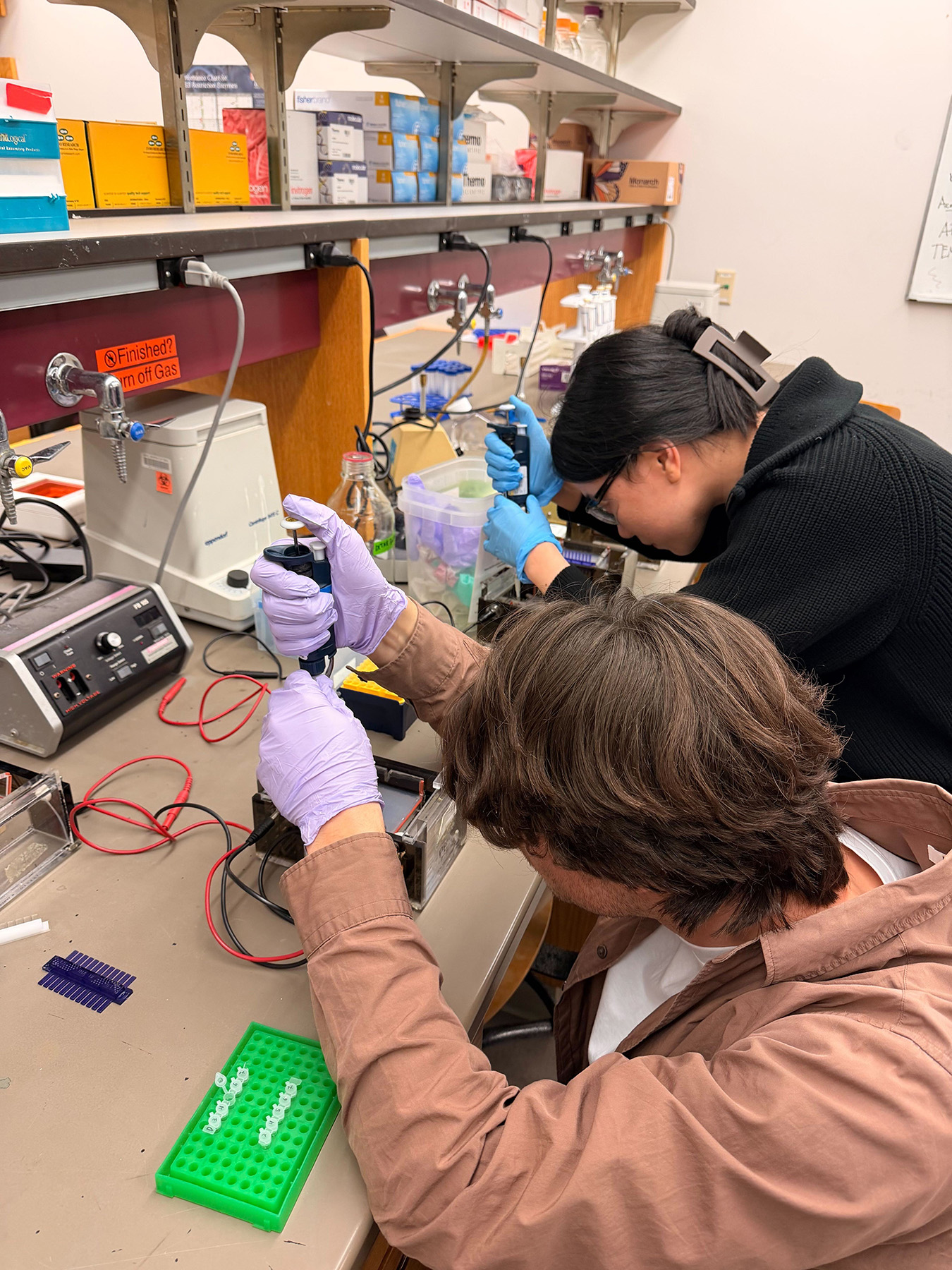
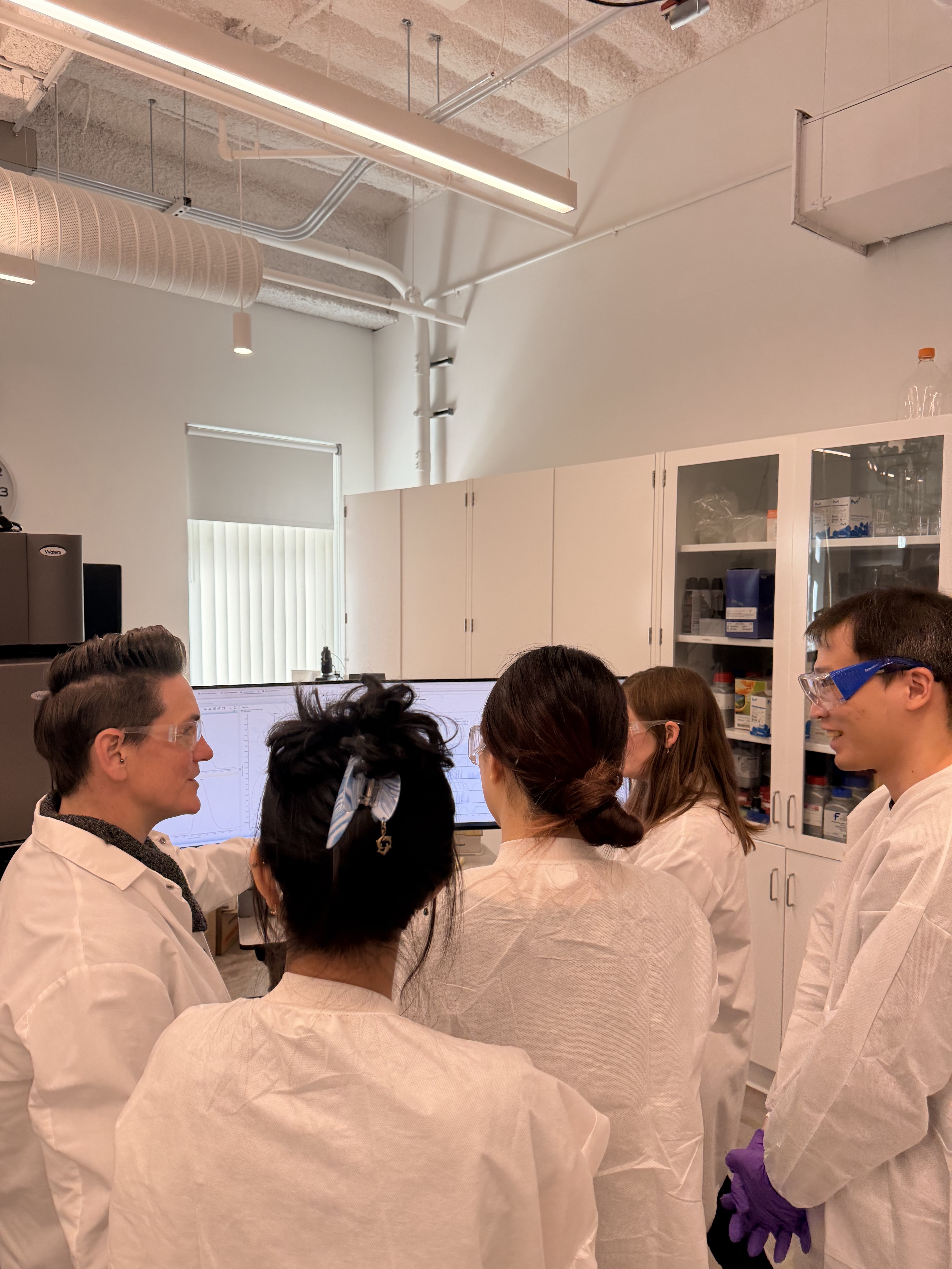
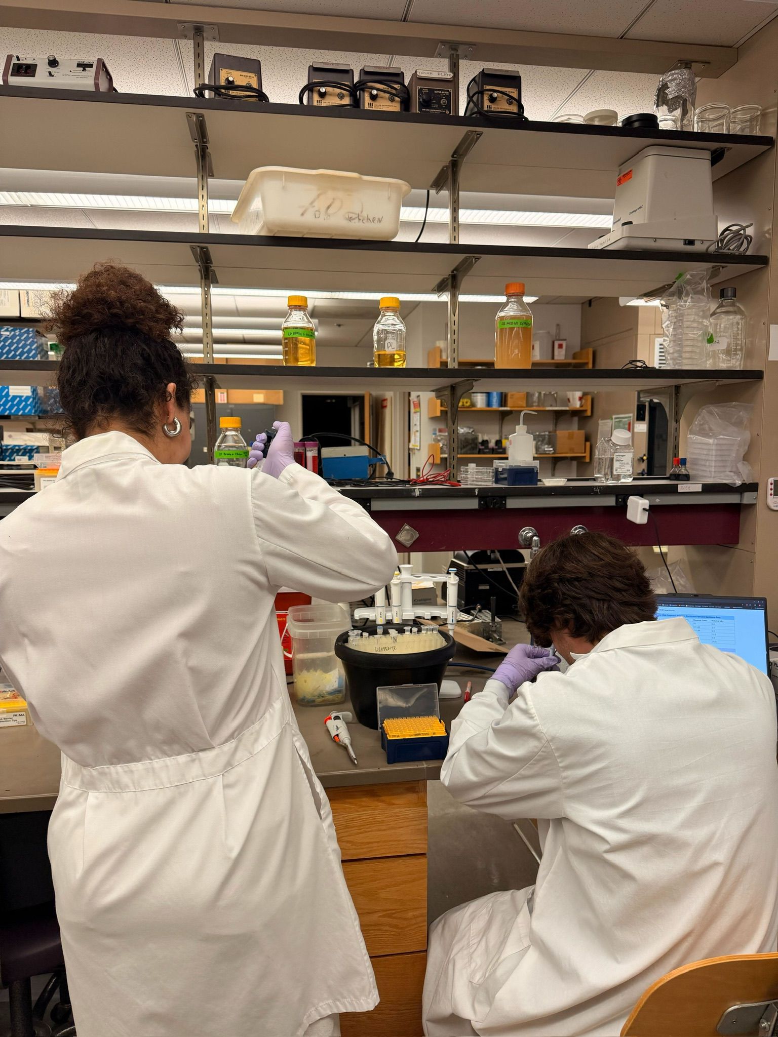
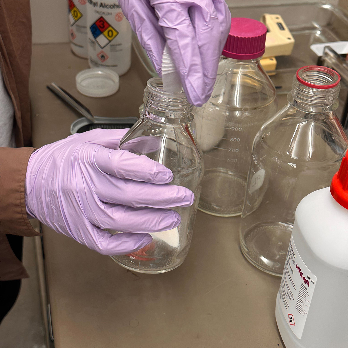
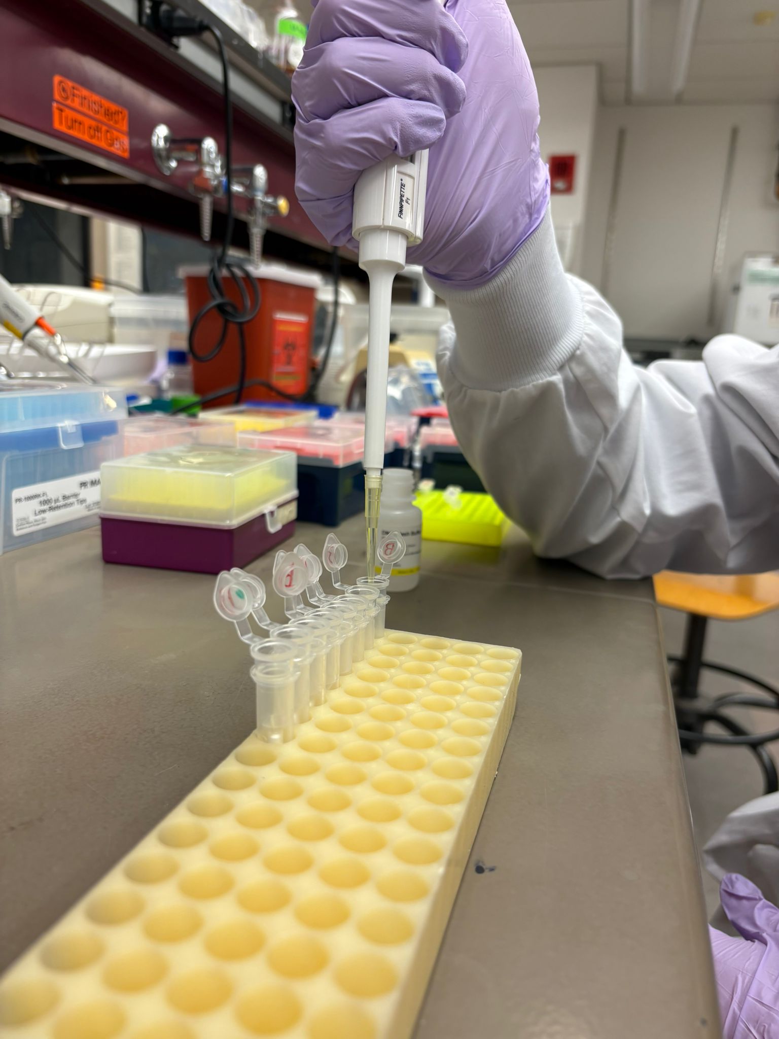
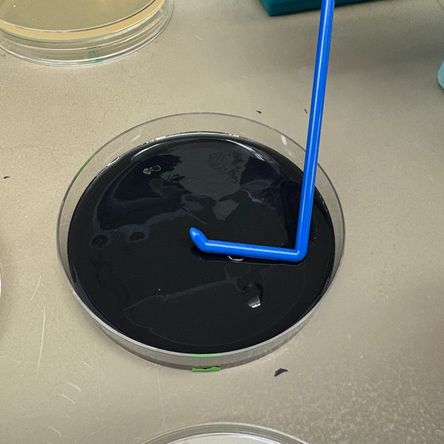
This week’s lab was about getting familiar with cuttind-edge lab automation tools. We were introduced to the Opentron, which to me was a close relative to 3d printing hardware and other gantry based fabrication method. It runs on a python script indicating coordinates for the working head to go-to, and has a pump and a motor where you would imagine the filament extruder motor and the heating element to be in a standard FDM 3d printer. Really enjoyed using this cool device.

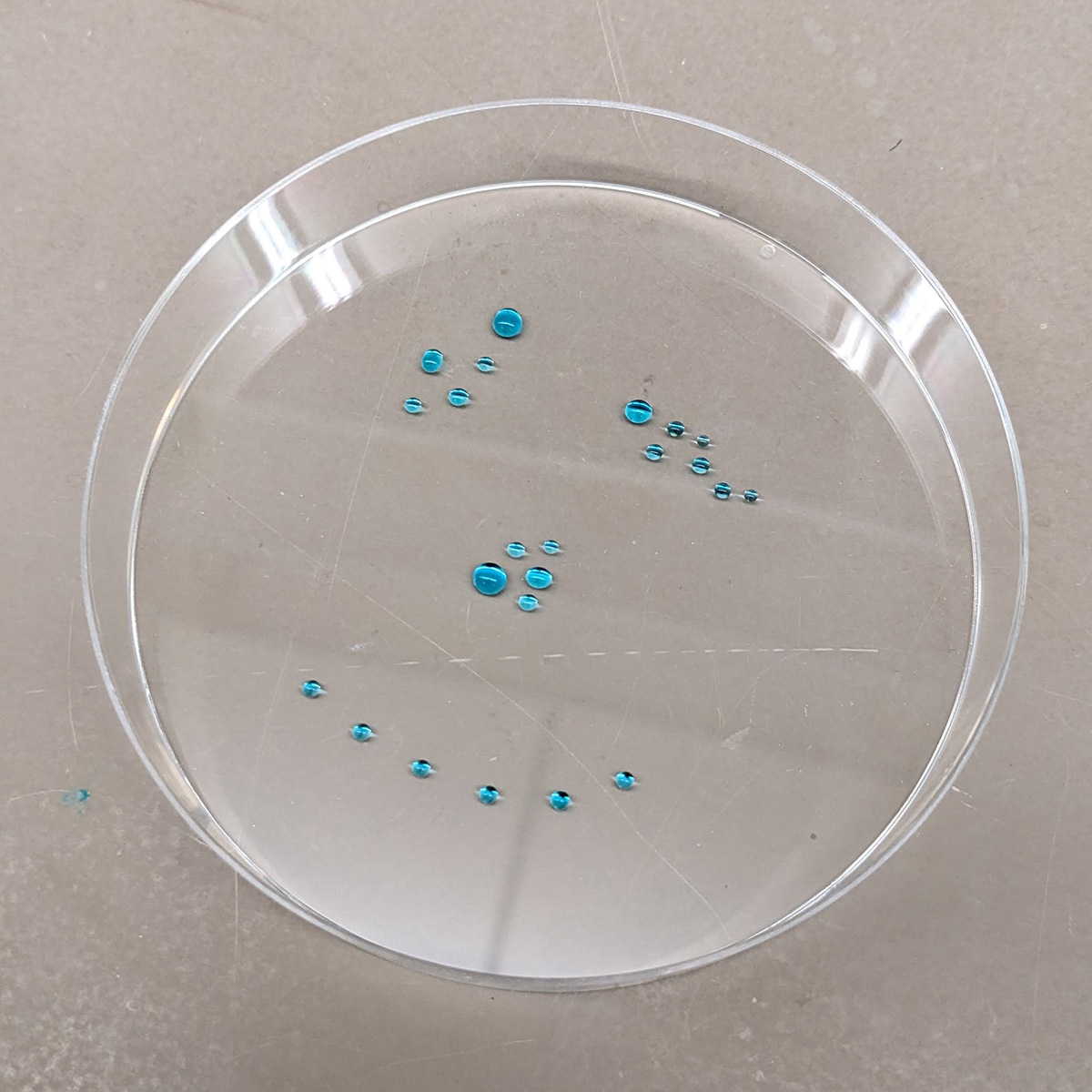
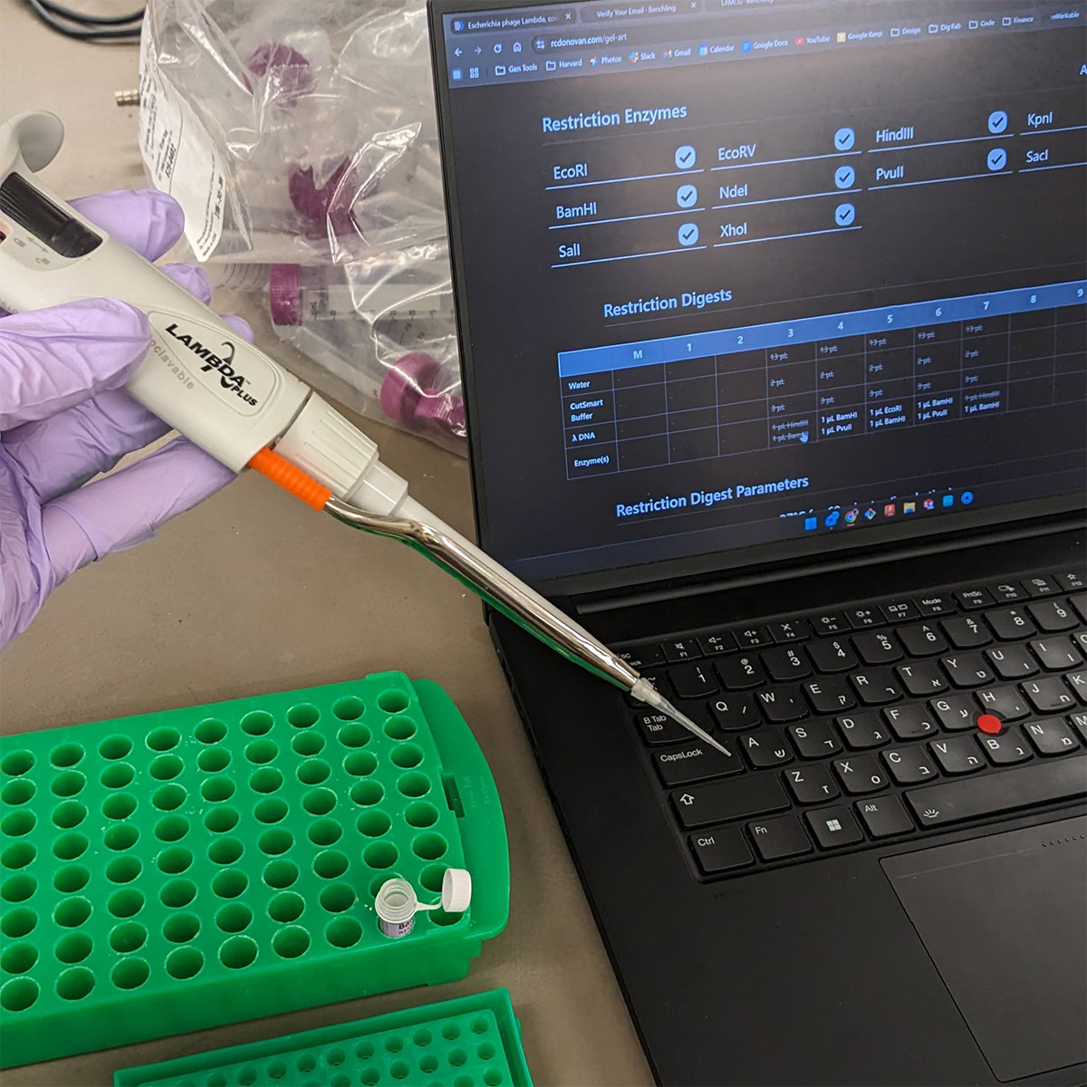
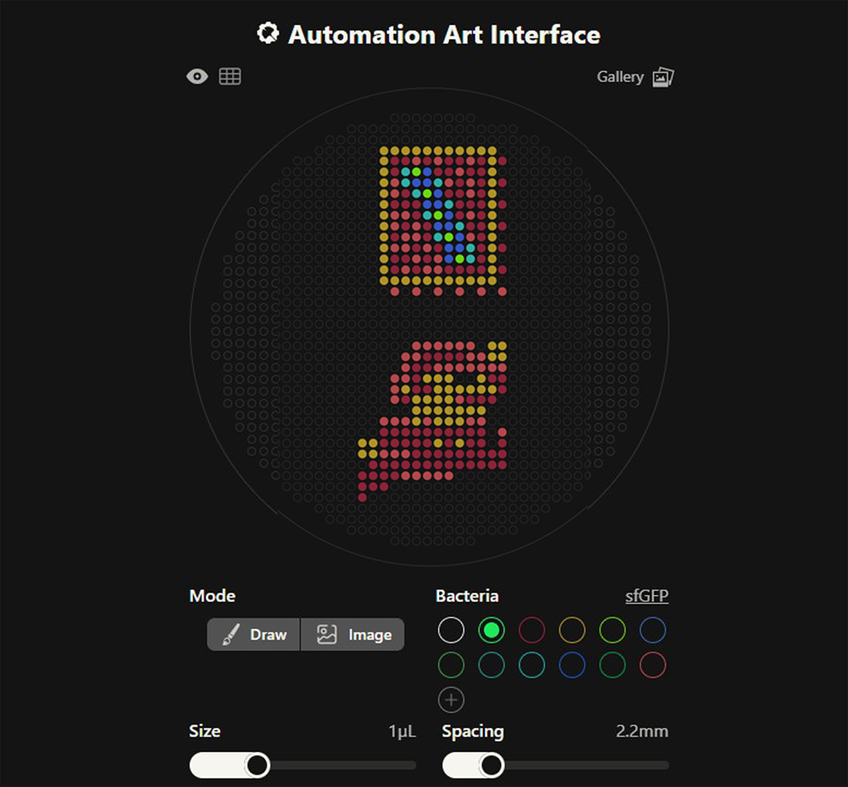
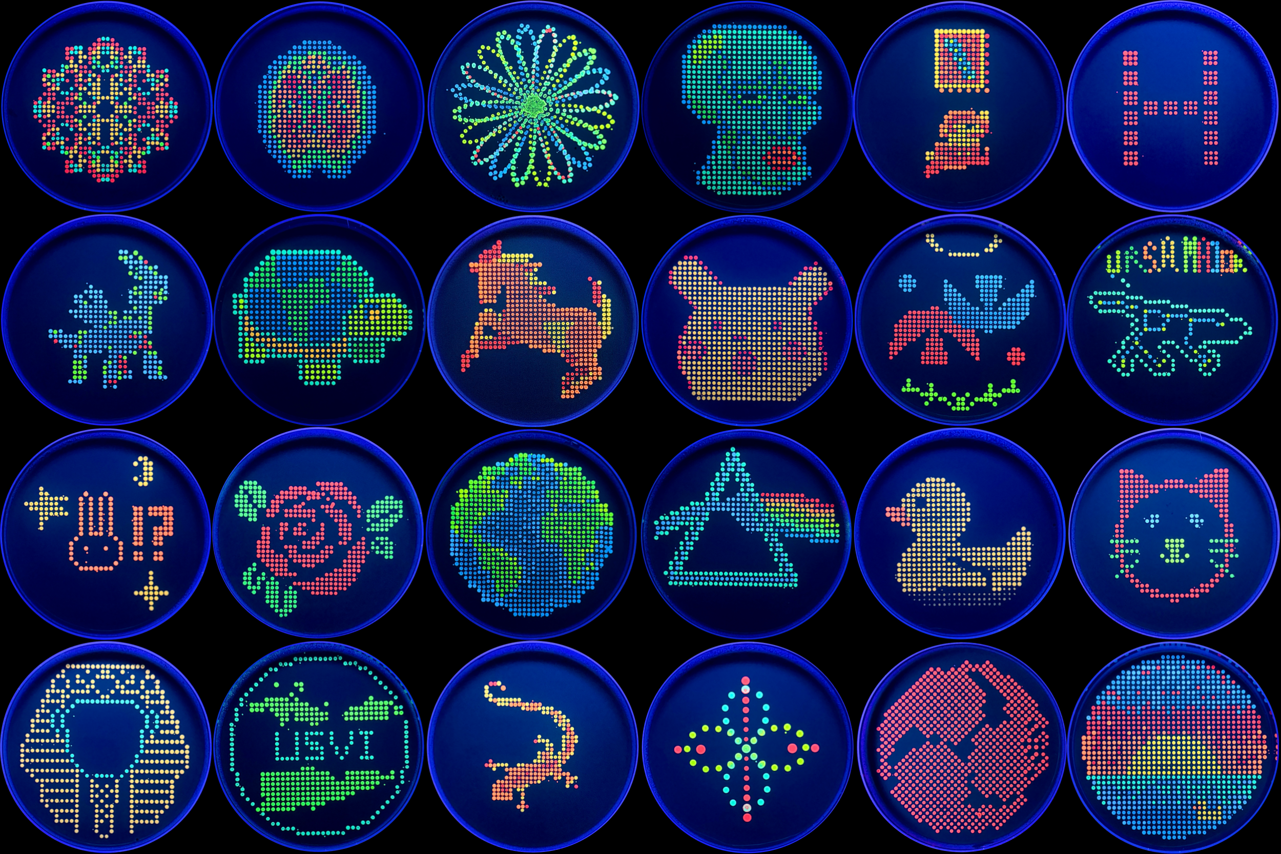
Thanks to Ronan Donovan’s awesome online tool, we could generate python scripts very quickly using a simple UI that translated our graphics into the code itself, very similar to what a slicer software does for an STL file to a 3D printer or what a CAM engine does for a STEP file for CNC operations.

Using the interface to create the script

the script:

from opentrons import types

import string

metadata = {
    'protocolName': '{YOUR NAME} - Opentrons Art - HTGAA',
    'author': 'HTGAA',
    'source': 'HTGAA 2026',
    'apiLevel': '2.20'
}

Z_VALUE_AGAR = 2.0
POINT_SIZE = 1

mrfp1_points = [(-7,31), (-5,31), (-1,31), (3,31), (5,31), (9,31), (13,31), (-7,29), (1,29), (3,29), (7,29), (9,29), (5,27), (9,27), (13,27), (-5,25), (3,25), (5,25), (9,25), (-7,23), (-5,23), (-3,23), (5,23), (7,23), (9,23), (13,23), (-3,21), (5,21), (9,21), (-5,19), (-1,19), (7,19), (9,19), (13,19), (-7,17), (-1,17), (9,17), (-3,15), (1,15), (9,15), (13,15), (-7,13), (-5,13), (-1,13), (9,13), (-7,11), (-3,11), (3,11), (5,11), (7,11), (9,11), (13,11), (-1,-5), (1,-5), (3,-5), (5,-5), (-3,-7), (-1,-7), (-3,-9), (11,-9), (13,-9), (-3,-11), (-1,-11), (13,-11), (-5,-13), (7,-13), (9,-13), (11,-13), (-9,-19), (-7,-19), (-5,-19), (-3,-19), (-1,-19), (1,-19), (3,-19), (5,-19), (7,-19), (9,-19), (-9,-21), (-7,-21), (-5,-21), (-3,-21), (-1,-21), (3,-21), (7,-21), (9,-21), (13,-21), (-3,-23), (-1,-23), (1,-23), (3,-23), (5,-23), (7,-23), (9,-23), (11,-23), (13,-23), (-11,-25), (-9,-25), (-7,-25), (-5,-25), (-3,-25), (-1,-25), (1,-25), (3,-25), (5,-25), (7,-25), (9,-25), (11,-25), (13,-25), (-13,-27), (-11,-27), (-9,-27), (-7,-27), (-13,-29), (-11,-29), (-9,-29), (-13,-31)]
mko2_points = [(-9,33), (-7,33), (-5,33), (-3,33), (-1,33), (1,33), (3,33), (5,33), (7,33), (9,33), (11,33), (-9,31), (11,31), (-9,29), (11,29), (-9,27), (11,27), (-9,25), (11,25), (-9,23), (11,23), (-9,21), (11,21), (-9,19), (11,19), (-9,17), (11,17), (-9,15), (11,15), (-9,13), (11,13), (-9,11), (11,11), (-9,9), (-7,9), (-5,9), (-3,9), (-1,9), (1,9), (3,9), (5,9), (7,9), (9,9), (11,9), (11,-3), (13,-3), (11,-5), (13,-5), (-1,-9), (1,-9), (3,-9), (9,-9), (-5,-11), (1,-11), (3,-11), (5,-11), (7,-11), (9,-11), (11,-11), (-3,-13), (-1,-13), (1,-13), (3,-13), (-3,-15), (-1,-15), (1,-15), (3,-15), (5,-15), (7,-15), (9,-15), (-3,-17), (1,-17), (3,-17), (5,-17), (-13,-21), (-11,-21), (1,-21), (5,-21), (-13,-23), (-11,-23)]
mscarlet_i_points = [(-3,31), (1,31), (7,31), (5,29), (-7,27), (3,27), (7,27), (-7,25), (7,25), (-7,21), (-5,21), (7,21), (-7,19), (-3,19), (-5,17), (-3,17), (7,17), (-7,15), (-5,15), (-1,15), (-3,13), (1,13), (-5,11), (-1,11), (1,11), (-7,7), (-3,7), (1,7), (5,7), (9,7), (13,7), (-3,-3), (-1,-3), (1,-3), (3,-3), (5,-3), (7,-3), (-5,-5), (-3,-5), (7,-5), (9,-5), (-5,-7), (1,-7), (3,-7), (5,-7), (7,-7), (9,-7), (11,-7), (13,-7), (-7,-9), (-5,-9), (-7,-11), (-7,-13), (5,-13), (-9,-17), (-7,-17), (-5,-17), (-1,-17), (7,-17), (9,-17), (13,-19), (-9,-23), (-7,-23), (-5,-23), (-5,-27), (-3,-27), (-1,-27), (1,-27), (3,-27)]
electra2_points = [(-1,29), (-3,27), (-1,27), (1,25), (-1,23), (1,23), (3,21), (1,19), (3,19), (5,17), (3,15), (5,15), (3,13)]
mturquoise2_points = [(-5,29), (-5,27), (1,27), (-3,25), (3,23), (-1,21), (5,19), (1,17), (7,15), (7,13)]
venus_points = [(-3,29), (-1,25), (1,21), (3,17), (5,13)]

point_name_pairing = [("mrfp1", mrfp1_points),("mko2", mko2_points),("mscarlet_i", mscarlet_i_points),("electra2", electra2_points),("mturquoise2", mturquoise2_points),("venus", venus_points)]

# Robot deck setup constants
TIP_RACK_DECK_SLOT = 9
COLORS_DECK_SLOT = 6
AGAR_DECK_SLOT = 5
PIPETTE_STARTING_TIP_WELL = 'A1'

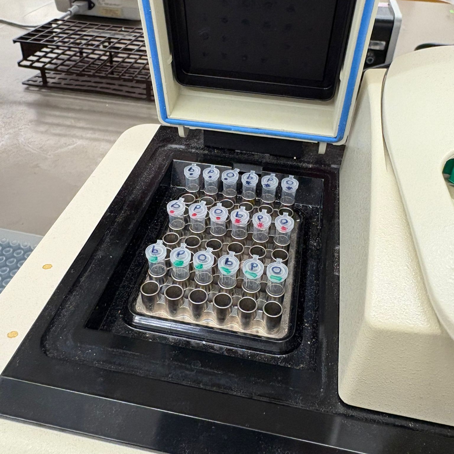
# Place the PCR tubes in this order
well_colors = {
    'A1': 'sfGFP',
    'A2': 'mRFP1',
    'A3': 'mKO2',
    'A4': 'Venus',
    'A5': 'mKate2_TF',
    'A6': 'Azurite',
    'A7': 'mCerulean3',
    'A8': 'mClover3',
    'A9': 'mJuniper',
    'A10': 'mTurquoise2',
    'A11': 'mBanana',
    'A12': 'mPlum',
    'B1': 'Electra2',
    'B2': 'mWasabi',
    'B3': 'mScarlet_I',
    'B4': 'mPapaya',
    'B5': 'eqFP578',
    'B6': 'tdTomato',
    'B7': 'DsRed',
    'B8': 'mKate2',
    'B9': 'EGFP',
    'B10': 'mRuby2',
    'B11': 'TagBFP',
    'B12': 'mChartreuse_TF',
    'C1': 'mLychee_TF',
    'C2': 'mTagBFP2',
    'C3': 'mEGFP',
    'C4': 'mNeonGreen',
    'C5': 'mAzamiGreen',
    'C6': 'mWatermelon',
    'C7': 'avGFP',
    'C8': 'mCitrine',
    'C9': 'mVenus',
    'C10': 'mCherry',
    'C11': 'mHoneydew',
    'C12': 'TagRFP',
    'D1': 'mTFP1',
    'D2': 'Ultramarine',
    'D3': 'ZsGreen1',
    'D4': 'mMiCy',
    'D5': 'mStayGold2',
    'D6': 'PA_GFP'
}

volume_used = {
    'mrfp1': 0,
    'mko2': 0,
    'mscarlet_i': 0,
    'electra2': 0,
    'mturquoise2': 0,
    'venus': 0
}

def update_volume_remaining(current_color, quantity_to_aspirate):
    rows = string.ascii_uppercase
    for well, color in list(well_colors.items()):
        if color == current_color:
            if (volume_used[current_color] + quantity_to_aspirate) > 250:
                # Move to next well horizontally by advancing row letter, keeping column number
                row = well[0]
                col = well[1:]
                
                # Find next row letter
                next_row = rows[rows.index(row) + 1]
                next_well = f"{next_row}{col}"
                
                del well_colors[well]
                well_colors[next_well] = current_color
                volume_used[current_color] = quantity_to_aspirate
            else:
                volume_used[current_color] += quantity_to_aspirate
            break

def run(protocol):
    # Load labware, modules and pipettes
    protocol.home()

    # Tips
    tips_20ul = protocol.load_labware('opentrons_96_tiprack_20ul', TIP_RACK_DECK_SLOT, 'Opentrons 20uL Tips')

    # Pipettes
    pipette_20ul = protocol.load_instrument("p20_single_gen2", "right", [tips_20ul])

    # PCR Plate
    temperature_plate = protocol.load_labware('opentrons_96_aluminumblock_generic_pcr_strip_200ul', 6)

    # Agar Plate
    agar_plate = protocol.load_labware('htgaa_agar_plate', AGAR_DECK_SLOT, 'Agar Plate')
    agar_plate.set_offset(x=0.00, y=0.00, z=Z_VALUE_AGAR)

    # Get the top-center of the plate, make sure the plate was calibrated before running this
    center_location = agar_plate['A1'].top()

    pipette_20ul.starting_tip = tips_20ul.well(PIPETTE_STARTING_TIP_WELL)
    
    # Helper function (dispensing)
    def dispense_and_jog(pipette, volume, location):
        assert(isinstance(volume, (int, float)))
        # Go above the location
        above_location = location.move(types.Point(z=location.point.z + 2))
        pipette.move_to(above_location)
        # Go downwards and dispense
        pipette.dispense(volume, location)
        # Go upwards to avoid smearing
        pipette.move_to(above_location)

    # Helper function (color location)
    def location_of_color(color_string):
        for well,color in well_colors.items():
            if color.lower() == color_string.lower():
                return temperature_plate[well]
        raise ValueError(f"No well found with color {color_string}")

    # Print pattern by iterating over lists
    for i, (current_color, point_list) in enumerate(point_name_pairing):
        # Skip the rest of the loop if the list is empty
        if not point_list:
            continue

        # Get the tip for this run, set the bacteria color, and the aspirate bacteria of choice
        pipette_20ul.pick_up_tip()
        max_aspirate = int(18 // POINT_SIZE) * POINT_SIZE
        quantity_to_aspirate = min(len(point_list)*POINT_SIZE, max_aspirate)
        update_volume_remaining(current_color, quantity_to_aspirate)
        pipette_20ul.aspirate(quantity_to_aspirate, location_of_color(current_color))

        # Iterate over the current points list and dispense them, refilling along the way
        for i in range(len(point_list)):
            x, y = point_list[i]
            adjusted_location = center_location.move(types.Point(x, y))

            dispense_and_jog(pipette_20ul, POINT_SIZE, adjusted_location)
            
            if pipette_20ul.current_volume == 0 and len(point_list[i+1:]) > 0:
                quantity_to_aspirate = min(len(point_list[i:])*POINT_SIZE, max_aspirate)
                update_volume_remaining(current_color, quantity_to_aspirate)
                pipette_20ul.aspirate(quantity_to_aspirate, location_of_color(current_color))

        # Drop tip between each color
        pipette_20ul.drop_tip()

The result:

Week 6 Lab: Gibson Assembly

This week our lab was about the Gibson Assembly process. We edited an exisiting plasmid by fragmenting it and ‘stiching’ it back with a mutated fragment. Our goal was to introduce a mutation of the chromophore of amilCP - a purple chromoprotein originally from the coral Acropora millepora - to generate new color variants that would be expressed in E.Coli bacteria. We did so by using PCR primers that already had the color mutations incorporated, and assembled it into a plasmid containing the elements needed for replication and expression in bacteria. The plasmid was then transformed into E. coli so the cells grow and express the mutated protein.

I teamed up with Libi for this lab, where we enjoyed applying the theory we learned throughout the course on the bench. The colorful results that were obtained demonstrate the importance of hands on learning and establishing the connecting link between theory and informed practice.

Amplifying reagents

The first step of the experiment was to amplify the plasmid containing the amilCP gene and the primer-mutations using PCR. We started with a plasmid that already contained the entire genetic circuit (the original color, along with the necessary elements for replication and expression.) Using different forward primers - correlating with the different expressed colors - and a rev primer as a general ‘cutter’, we introduced mutations in the chromophore region of the gene while amplifying the DNA. The PCR reactions were designed so that the plasmid (circular) was effectively split into two linear fragments: a longer fragment: the plasmid backbone where we would reintroduce mutated genes, and the shorter linear fragment containing only the mutated gene.

We chose to try and create the orange, blue, and light pink mutations of the gene. Each of us prepared our own PCR mixtures — Libi nicely prepared one backbone reaction along with the three color variants, while I got distracted and accidentally prepared four backbone reactions (:

After preparing the reactions, the tubes were briefly centrifuged and placed in the thermocycler, which carried out repeated cycles of denaturation, primer annealing, and extension to amplify the desired DNA fragments.

The full compositions and concentrations for each PCR reaction are summarized in the tables below.

Gel running

To make sure our PCR was done properly (we amplifyed what we assumed we were amplifying) we ran one of my backbones (now refered to as BackboneAsaf or BA in short) alongside Libi’s backbone (now refered to as BackboneLibi or BL in short) and the 3 ampifyed mutations for the chosen colors, with a ladder well in both the M and 10 slots for reference. Rest of the wells were filled with water.

We obtained the expected fragments for the orange and blue variants, as well as for both backbone reactions (BL and BA). However, we did not observe a band in the light pink lane, suggesting that something likely went wrong during that PCR reaction. Despite this, we continued to carry the light pink sample through the rest of the protocol.

DNA washing

After verifying the PCR products on the gel, we proceeded with DNA cleanup using a Zymo spin-column purification kit: For each sample, we added DNA binding buffer at a 5:1 ratio relative to the PCR product volume and mixed the solution. We then proceeded to vortexing the mix in a specialised doulbe tube configuration where the desired product would get absorbed in a hydrogel bead while the rest of it gets spun out to an external enveloping tube.

We performed the wash step using DNA wash buffer, centrifuging after each wash and repeating this step twice to ensure proper purification of the DNA.

Finally, the DNA was eluted from the column using elution buffer, resulting in purified PCR products ready for downstream applications.

Here are the results we had at the end of the first day of this lab:

The image shows the PCR products for the three color variants and five backbone reactions, the diluted PCR products for the three colors along with BA and BL, and the cleaned PCR products for all reactions. In the labeling, BA is marked as “B” with a green dot, while BL is marked as “B” with a purple dot.

At the end of the day, we stored the purified DNA samples in the fridge and continued the experiment the following day.

Concentration Measurement – Nanodrop

We started the second day by using a NanoDrop spectrophotometer to measure the DNA concentration of our cleaned samples. For each measurement, we loaded 2 µL of sample onto the machine.

We first measured one of the cleaned backup backbone samples and obtained the following result:

As shown, the concentration was 8.7 µg/mL, which is significantly lower than the values we expected (around ~20 µg/mL).

We then measured another cleaned backbone sample, this time BL, which gave a slightly better result of 12.5 µg/mL, but still lower than desired.

At this point, we decided to measure the concentration directly from the original PCR products (without cleanup). We first tested the BA PCR sample and obtained a much higher reading of 449.5 µg/mL:

We then measured the BL PCR sample, which showed a concentration of 486.2 µg/mL:

These values are likely overestimates of the true DNA concentration due to the presence of primers, nucleotides, and other components in the PCR mixture. However, they were clearly much higher than the cleaned samples, suggesting that the cleanup step may have resulted in significant DNA loss.

Gibson Assembly

For this part, we used Gibson Assembly to recombine the PCR-generated fragments into complete plasmids. We designed 6 different assemblies for each color variant (18 total), varying three main parameters:

DNA source: cleaned vs. uncleaned PCR product (referred to as PCR) Backbone type: BL for PCR samples, and both BL and BA for cleaned samples Assembly composition: either according to the standard protocol or a modified version (x2) to compensate for the low DNA concentrations observed after cleanup

The standard assembly mixture (based on the protocol) was:

To account for the low concentrations observed after cleanup, we designed a modified version (x2):

All assembly combinations are summarized in the table below:

Legend: 💙 = Blue 🩷 = Light Pink 🧡 = Orange

We then prepared the different assembly reactions by pipetting the required components into labeled tubes.

After preparing the mixtures, the tubes were incubated to allow the fragments to assemble into complete plasmids.

Finally, the assembled plasmids were ready for transformation into E. coli.

Transformation

For this part, we transformed the assembled plasmids into competent E. coli cells. We added the Gibson assembly products to chemically competent cells and incubated the mixtures on ice for 30 minutes to allow the DNA to associate with the cells.

After heat shock (following the protocol), we added SOC medium to allow the cells to recover. While the protocol suggests 200–500 µL, we used 150 µL of SOC for each sample per Ronan’s reccomendation.

The tubes were then placed in a shaking incubator to promote recovery and expression of the antibiotic resistance gene.

We used standard DH5α competent cells for most transformations. However, for the orange, cleaned BL, x2 assembly, we also used 10-beta competent cells to boost transformation efficiency. In addition, we performed a separate transformation of the orange PCR BL (standard concentration) using only 10-beta cells. In total, we performed 19 transformations.

After the 60 minute growth period in the shaking incubator, we proceeded with plating the transformed cells onto agar plates.

For the cleaned BL and PCR BL assemblies (both concentrations), we divided standard agar plates into thirds and plated a different color variant in each section. We also prepared a plate containing a mixture of all three colors from the BA cleaned DNA x2 assembly (we called it MIX).

We then used charcoal agar plates from the Opentrons art lab to create additional plates, since we observed some background growth on the regular plates from a control that was done earlier (colonies that likely did not take up the plasmid). We therefore wanted to use plates that we knew provide more reliable selection, and also explore the improved visual contrast offered by the charcoal medium.

For each assembly type, we again divided the plates into thirds and plated a different color in each section, this time for all assemblies. In addition, we prepared:

A mixed plate of all three colors from the BL cleaned DNA x2 assembly A plate containing only the orange PCR BL (10-beta only) transformation For plates containing all three colors, we plated 40 µL of each sample. For plates containing a single sample, we plated 100 µL.

Finally, the plates were incubated for approximately 36 hours to allow colony growth.

Results

After 36 hours, the plates were taken out of the incubator and stored in the fridge.

Overall, we successfully completed the experiment. The mutation that performed best across the different assemblies was blue, followed by orange (with slightly less consistent success across plates). As expected from the gel results, the light pink variant did not appear in any of the plates, except for one potential colony on the MIX BL clean x2 plate. However, it is unlikely to be truly pink, since no corresponding signal was observed elsewhere.

The best overall result was obtained from the PCR, regular concentration, BL assembly, which produced many clear blue and orange colonies:

This result suggests that the uncleaned PCR samples actually performed better in the assembly, likely because they retained a much higher DNA concentration, while the cleanup step may have reduced the available DNA more than expected.

We observed slightly fewer colonies on the charcoal plates. This may suggest stronger selection conditions or differences in growth on the charcoal medium. However, these plates still provided useful results and allowed us to observe the colony colors against a dark background (although the contrast was somewhat less distinct than expected). Here as well, the best-performing condition was PCR, regular concentration, BL:

The special transformation using 10-beta competent cells for the orange variant was not successful overall, with only a single colony observed on the charcoal plate:

Here are the results we obtained across all plates:

Overall, this was a great experience. Seeing E. coli colonies appear in different colors was especially exciting, and it was very fun to apply techniques we had previously only learned about in theory. I’m excited to be able to practice such procedures for the first time, and I definetly learned a lot from it!