Week 10 HW: Imaging and Measurement
What will I measure?
My final project involves modifying an existing flowering plant species to enhance anthocyanin pigment production. So that’s metric number one. How much production is occurring. Now the reason we’re tweaking anthocyanin production is to turn the petals of the plant into reliable pH indicators. I would also need to measure the change in color, the rate of deterioration of pigment after plucking the petal. The correlation between temperature and pigment concentration and also the overall pigment concentration in petals, if it can be even roughly standardized (all petals might not have exact amount for it to function as intended. so we tweak and see if at least all petals have similar concentration and if not then what is the limiting factor (specific env. conditions?))
What would I like to measure and how ? I am not really about the entire list of elements but I have an idea. I would like to measure:
- total anthocyanin pigment concentrations in petals (HPLC-MS to identify the kinds of anthocyanins being produced) (to know if enough pigment is being produced to even have a color change)
- petals color response to pH, variablity between two petals/two plants (no idea, some type of colorimetry i guess. Taking known pH solutions to test) (to check if the plant even works reliably)
- pH response accuracy compared to high accuracy pH meters/litmus paper (create some sort of calibration curve and compare to pH meters) (to see how the petals compare to standard methods)
- some measure of the gene expression. (using RNA-seq? )(to check the expression level of the inserted/modified genes)
- metabolic activity / metabolomics (LC-MS to separate and identify metabolites) to optimize the anthocyanin synthesis pathway)
What technologies would I use? Mostly chromatographic techniques to separate and study the pigments, to study the metabolic activity. Techniques like RNA-seq will help me study the genes behind the metabolic pathways and look for ways to optimize/upregulate.
Side Note
While trying to figure out how to make this work, I came across a species of flowers ‘Clitoria ternatum’ also known as Butterfly Pea. The flower already shows a wide range of color change to changes in pH and that too across a large range. As the flower contains ternatins, one of the most stable anthocyanins, they show a color change across the 4-12 pH range which makes them pretty usable. I think they can be picked as the candidate species as only an upregulation of existing pathways and optimization and sterility induction could make the final project possible.
The flower already shows a wide range of color change to changes in pH and that too across a large range. As the flower contains ternatins, one of the most stable anthocyanins, they show a color change across the 4-12 pH range which makes them pretty usable. I think they can be picked as the candidate species as only an upregulation of existing pathways and optimization and sterility induction could make the final project possible.
I also found out that ternatins kill cancer cells and also inhibit fat accumulation, which led me to think maybe a tea from butterfly pea would help me with the easy fat that my body is genetically inclined to store and turns out Butterfly pea tea is a REAL THING!
Homework: Waters Part I — Molecular Weight
Q1
I took the eGFP sequence and went to the Expasy website’s pI (isoelectric point) and mw (molecular weight) calculator and pasted the sequence in there. The molecular weight I got was 27893.44 Dalton (The unit wasn’t specified on the website, I mean it was but in the documentation.)
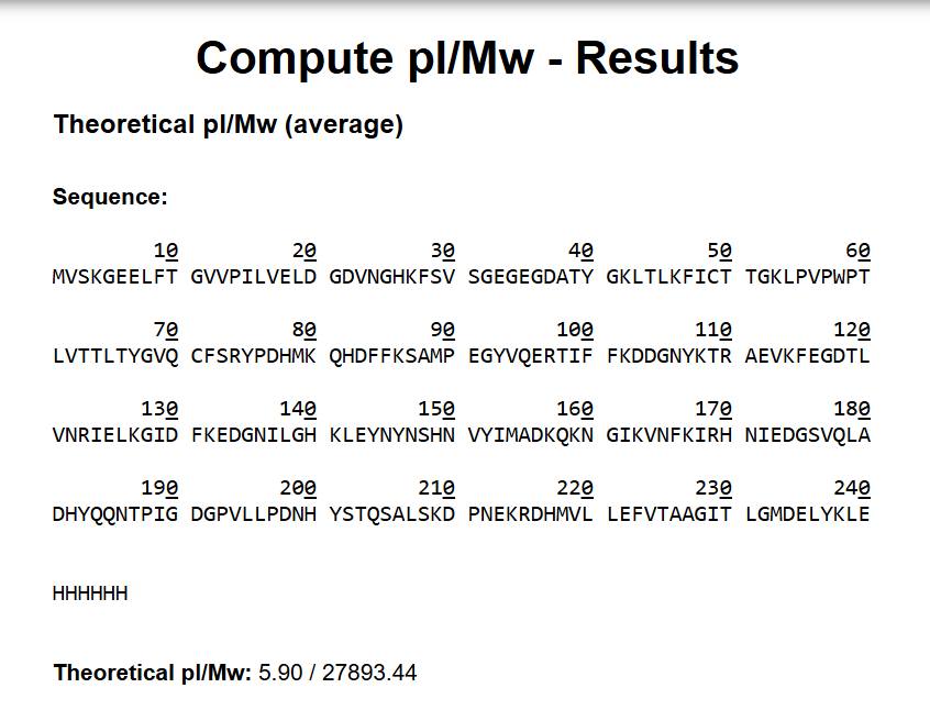 Molecular Weight with Le and HHHHHH (27893.44 Da)
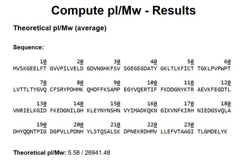 Molecular weight without the LE and HHHHHH (26941.48 Da)
Q2
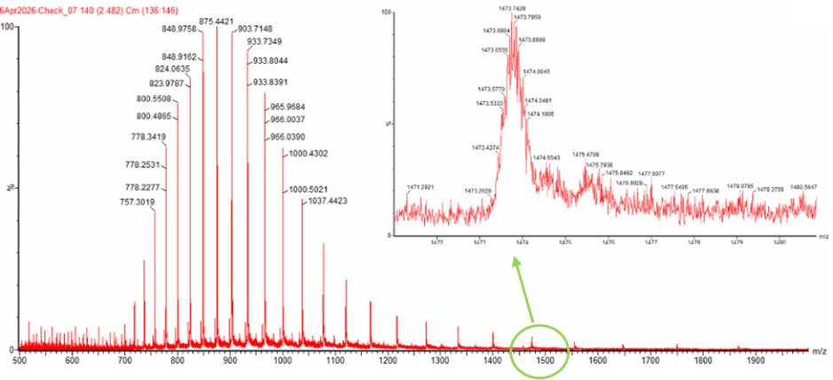
Next up was to calculate the molecular weight of eGFP using adjacent charge state approach. I calculated the molecular weight using adjacent charge state peak pairs read from Figure 1 (denatured eGFP, LC-MS).
 First determine z using the formula in the homework brief.
| Pair | m/zn(higher) | m/zn+1 (lower) | Difference | Calculated z | Rounded z |
|---|---|---|---|---|---|
| 1 | 903.7148 | 875.4421 | 28.2727 | 30.96 | 31 |
| 2 | 933.7349 | 903.7148 | 30.0201 | 30.10 | 30 |
| 3 | 965.9584 | 933.7349 | 32.2235 | 28.98 | 29 |
| 4 | 1000.4302 | 965.9584 | 34.4718 | 28.02 | 28 |
| 5 | 1037.4423 | 1000.4302 | 37.0121 | 27.03 | 27 |
| Then determine the mw from z and m/z using: |
| Peak m/zₙ | z | MW (Da) |
|---|---|---|
| 903.7148 | 31 | 27,983.9 |
| 933.7349 | 30 | 27,981.8 |
| 965.9584 | 29 | 27,983.5 |
| 1000.4302 | 28 | 27,983.8 |
| 1037.4423 | 27 | 27,983.7 |
Now we calculate the average of these values to get experimental molecular weight.
The value we get is 27983.39 Da, which is super close to the value we computed using Expasy’s calculator. Next step is to calculate the accuracy of the measurement.
Q3
The peak near m/z 1474 also fits well with a charge state of 19+. Based on the measured molecular weight, a 19+ ion should appear at about m/z 1473.8, which is very close to the observed peak position. Therefore, the zoomed-in peak is most likely a z = 19 ion.
Homework: Waters Part II — Secondary/Tertiary structure
Q1 In the folded state, the protein keeps its compact 3D structure, so fewer protonation sites are exposed. As a result, it carries fewer charges and appears at higher m/z values with a narrow charge-state distribution in the mass spectrum. In the denatured state, the protein chain opens up and more basic residues become exposed. This allows the protein to carry more charges, producing peaks at lower m/z values with a broader charge-state distribution
In Figure 2, the native spectrum (bottom, red) shows only a few peaks at high m/z, indicating a folded protein with low charge states. The denatured spectrum (top, green) shows many peaks spread across lower m/z values, indicating an unfolded protein with high charge states.
Q2
Using the two adjacent peaks at m/z 2799.4199 and 2545.0388, the charge state of the ~2800 peak is calculated to be z = 10. Therefore, the ~2545 peak corresponds to z = 11.
Both charge states give a molecular weight of about 27,984 Da, which closely matches the theoretical value.
Homework: Waters Part III — Peptide Mapping - primary structure
Q1
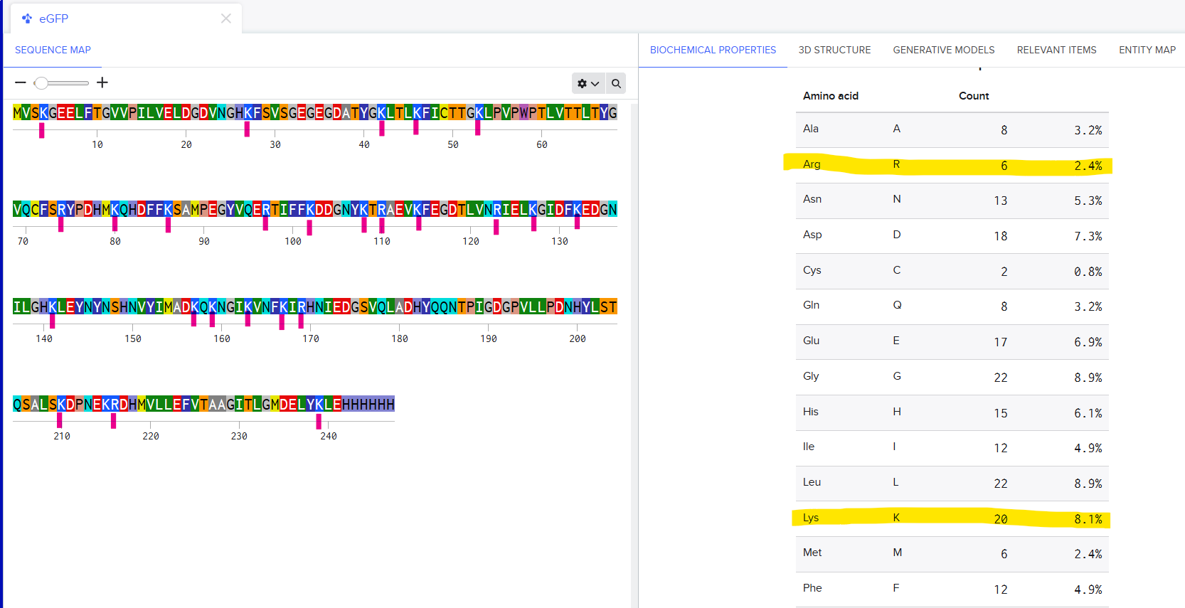
There are 6 Arginines and 20 Lysines in eGFP. I imported the sequence into Benchling and saw the count for amino acids in the Biochemical Propeties Tab.
Q2
I copied the sequence for eGFP and went to the Expasy’s Peptide Mass Tool to find out how many peptides will be generated from tryptic digestion of eGFP. I pasted the sequence in the input box and used the screenshot from the homework brief to select other relevant parameters. ([M+H]+ , monoisotopic, Trypsin, 500-unlimited Da, peptide masses or in, all known post-translational modifications) (tbh they’re were already selected as is.)
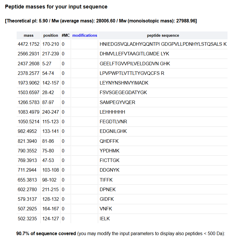
This is the result that I got. There were about 19 peptides generated.
Q3
Counting all labeled peaks between 0.5 and 6.0 min with > 10% relative abundance there’s about 18-20 peaks.
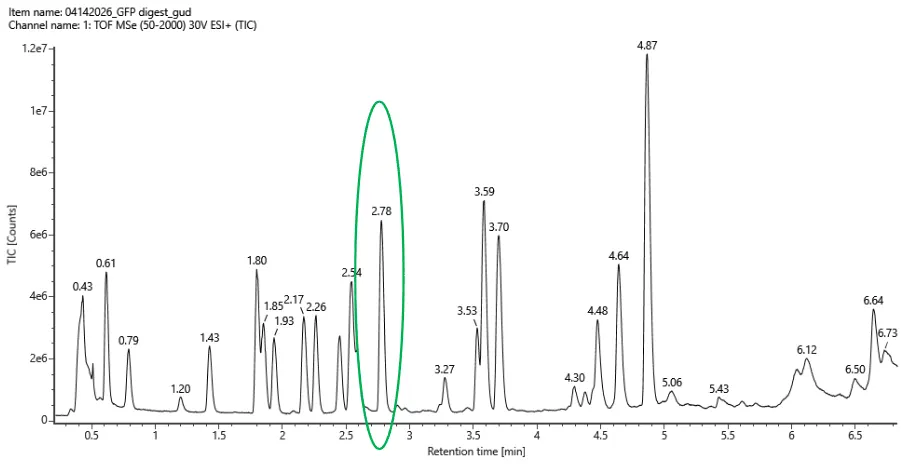 Fig 5a
Q4
The number of predicted peaks was 19 and the amount of peaks are 18-20. There are more peaks in the chromatogram. But overall, the peptide map is consistent with the predicted peptides.
Q5
The most abundant peak in the mass spectrum of the 2.78 min fraction is at:
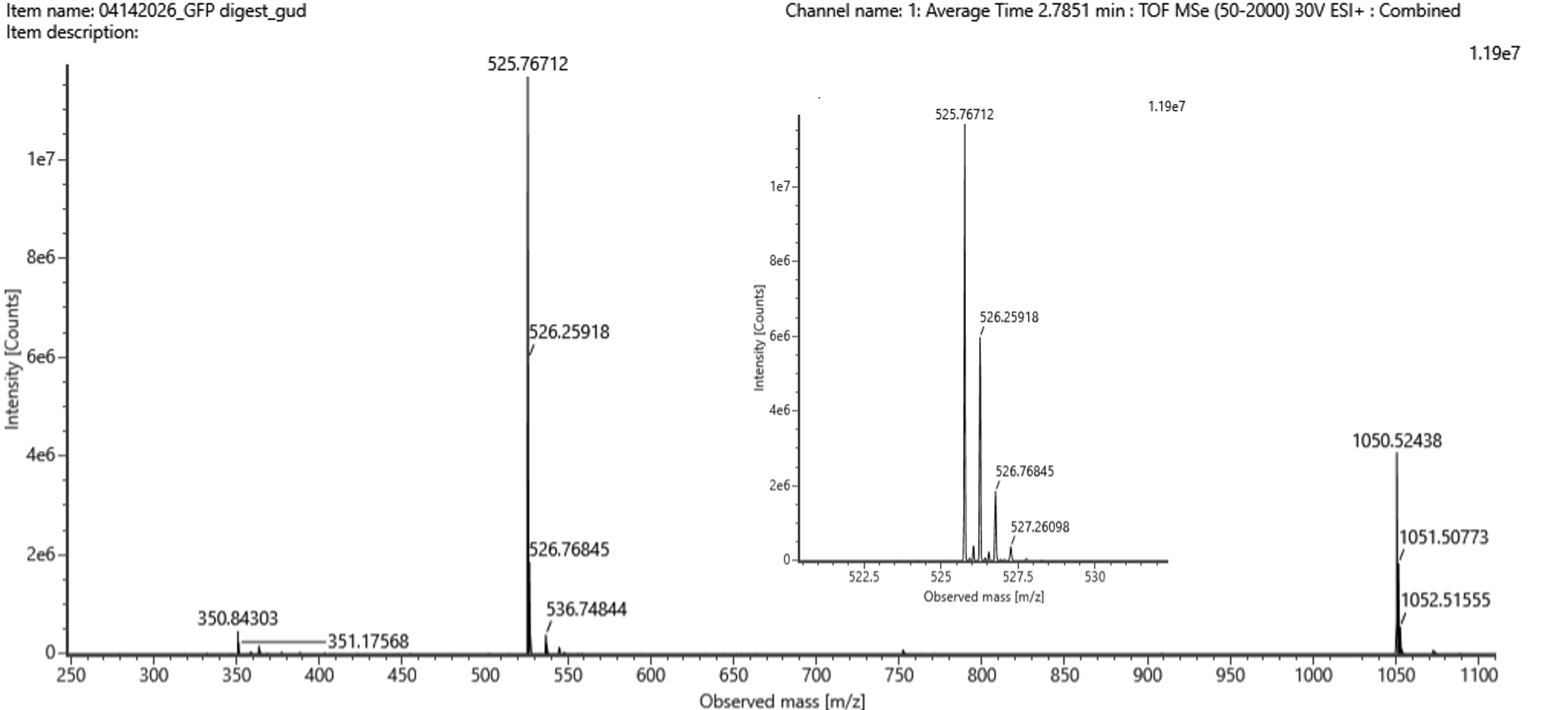 Fig 5b
Determining the charge state from isotope spacing
So, an isotope spacing of approximately 0.5 m/z indicates a charge state of:
Calculating the singly charged mass
Confirmation
The peak at:
matches the calculated singly charged mass, confirming that it is the singly charged form of the same peptide.
Q6
Searching the PeptideMass output for [M+H]⁺ ≈ 1050.527 Da, we find out that the closest to that mass is the peptide: FEGDTLVNR. The theoretical mass (from peptide mass tool) was 1050.5214. The calculated mass was 1050.527. A difference of 0.006.
Q7
Figure 6 shows that the amino acid coverage of eGFP is 88%. This means that 88% of the eGFP sequence was confirmed by peptide mapping.
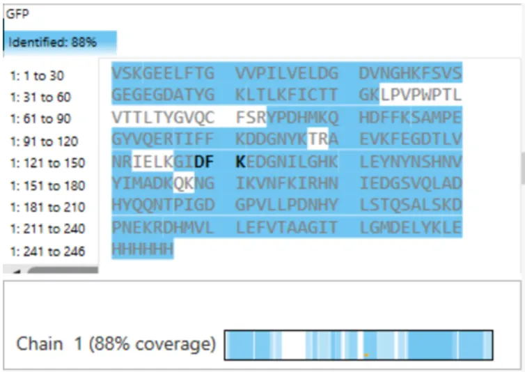 Fig 6
Fig 6
Homework: Waters Part IV — Oligomers
We will determine Keyhole Limpet Hemocyanin (KLH)’s oligomeric states using charge detection mass spectrometry (CDMS). CDMS single-particle measurements of KLH allow us to make direct mass measurements to determine what oligomeric states (that is, how many protein subunits combine) are present in solution. Using the known masses of the polypeptide subunits (Table 1) for KLH, identify where the following oligomeric species are on the spectrum shown below from the CDMS (Figure 7):
- 7FU Decamer
- 8FU Didecamer
- 8FU 3-Decamer
- 8FU 4-Decamer
| Polypeptide Subunit Name | Subunit Mass |
|---|---|
| 7FU | 340 kDa |
| 8FU | 400 kDa |
Predicted Masses of the Four Oligomeric Species
Each “decamer” unit = 10 polypeptide chains. Larger assemblies are multiples of this:
| Oligomeric Species | Formula | Predicted Mass |
|---|---|---|
| 7FU Decamer | 10 × 340 kDa | 3,400 kDa = 3.4 MDa |
| 8FU Didecamer | 20 × 400 kDa | 8,000 kDa = 8.0 MDa |
| 8FU 3-Decamer | 30 × 400 kDa | 12,000 kDa = 12.0 MDa |
| 8FU 4-Decamer | 40 × 400 kDa | 16,000 kDa = 16.0 MDa |
| Table 1: KLH Subunit Masses |
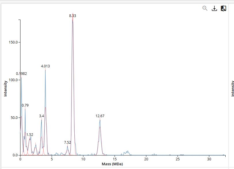
Figure 7. Mass spectrum of Keyhole Limpet Hemocyanin (KLH) acquired on the CDMS.
Assignment of Peaks in the CDMS Spectrum (Figure 7)
| Species | Predicted Mass | Observed Peak | Δ (%) |
|---|---|---|---|
| 7FU Decamer | 3.4 MDa | 3.4 MDa | 0.0% |
| 8FU Didecamer | 8.0 MDa | 8.33 MDa | +4.1% |
| 8FU 3-Decamer | 12.0 MDa | 12.67 MDa | +5.6% |
| 8FU 4-Decamer | 16.0 MDa | no labeled peak | — |
The 7FU Decamer gives a perfect match at 3.4 MDa - the labeled peak in Figure 7 at exactly 3.4 MDa is unambiguous.
The 8FU Didecamer and 3-Decamer match the 8.33 MDa and 12.67 MDa peaks with 4–6% deviation. These deviations are consistent and systematic both are higher than predicted by roughly the same factor, which is typical of CDMS calibration offsets for very large particles (>5 MDa). Notably:
The ratio of the measured masses closely follows the expected 3:2 ratio for a 3-Decamer vs. Didecamer, strongly confirming their identities.
The 8FU 4-Decamer (predicted 16.0 MDa) has no clearly labeled peak in Figure 7. The spectrum extends to ~30 MDa but shows minimal signal beyond ~13 MDa. This likely means the 4-Decamer is either not present in this KLH sample in significant abundance, or is present at levels below the detection threshold of the CDMS measurement.
Homework: Waters Part V — Did I make GFP?
| Parameter | Theoretical | Observed / Measured on Intact LC-MS | PPM Mass Error |
|---|---|---|---|
| Molecular weight (kDa) | 27893.44 Da | 27983.39 Da | 3225 ppm |