This week’s focus is on the intersection of biology, robotics, and creative coding. As part of the HTGAA 2026* cohort based in Zambia, I am exploring how liquid-handling automation (specifically the Opentrons OT-2) can streamline laboratory workflows. Beyond the technical utility, this assignment challenged us to use the robot as a canvas, translating digital coordinates into physical biological art.
Lab automation isn’t just about efficiency; it’s about precision in environments where resources must be used optimally. My work this week involves a Python-based protocol that instructs the robot to “paint” a design using colored liquids in a 96-well plate.
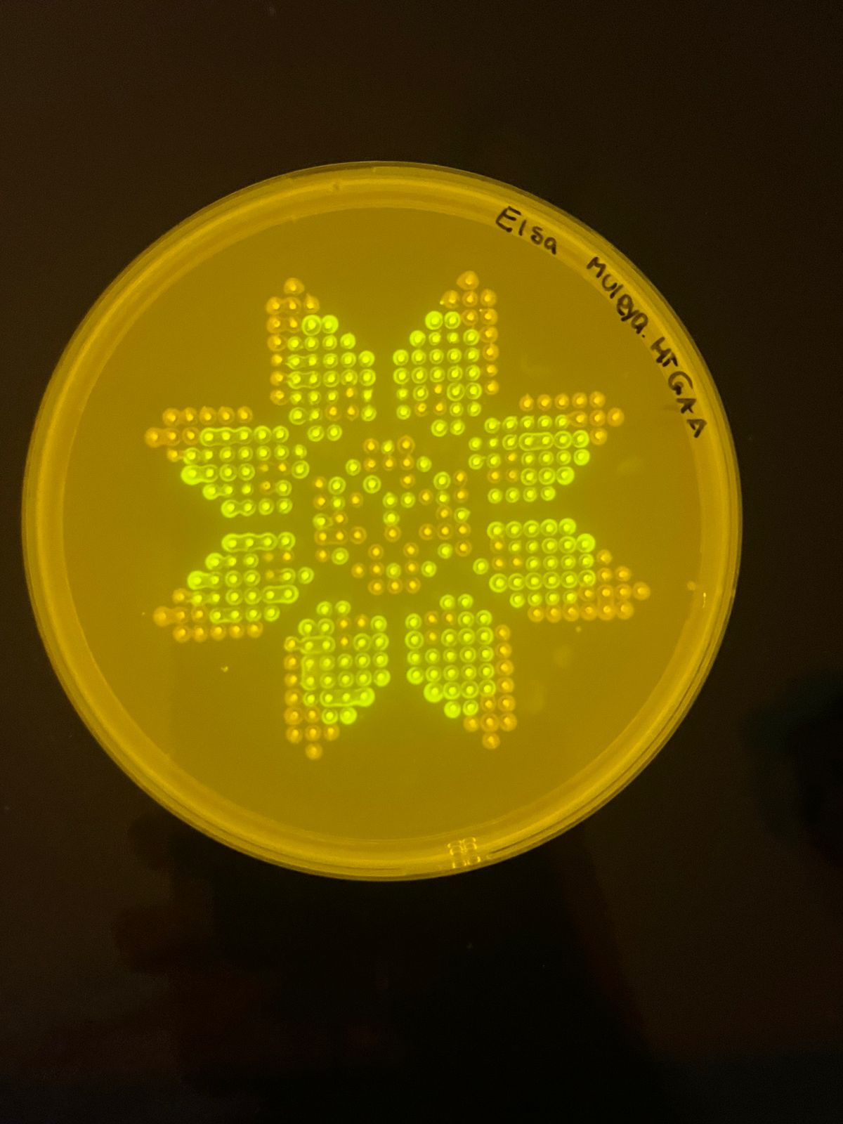
I used the Opentrons Art GUI to map out the coordinates for my design. The visual representation and the specific well-mapping for this protocol can be viewed at the link below:
Below is the Python script generated to execute the design. This script defines the labware (tips, reservoir, and plate) and the specific pipetting movements required to recreate the art.
from opentrons import types

metadata = {    # see https://docs.opentrons.com/v2/tutorial.html#tutorial-metadata
    'author': 'ELSA MULEYA',
    'protocolName': 'HTGAA Agar Art - Full Set',
    'description': 'FLORAL ART',
    'source': 'HTGAA 2026 Opentrons Lab',
    'apiLevel': '2.20'
}

##############################################################################
###   Robot deck setup constants - don't change these
##############################################################################

TIP_RACK_DECK_SLOT = 9
COLORS_DECK_SLOT = 6
AGAR_DECK_SLOT = 5
PIPETTE_STARTING_TIP_WELL = 'A1'

well_colors = {
    'A1' : 'Red',
    'B1' : 'Green',
    'C1' : 'Orange'
}


def run(protocol):
  ##############################################################################
  ###   Load labware, modules and pipettes
  ##############################################################################

  # Tips
  tips_20ul = protocol.load_labware('opentrons_96_tiprack_20ul', TIP_RACK_DECK_SLOT, 'Opentrons 20uL Tips')

  # Pipettes
  pipette_20ul = protocol.load_instrument("p20_single_gen2", "right", [tips_20ul])

  # Modules
  temperature_module = protocol.load_module('temperature module gen2', COLORS_DECK_SLOT)

  # Temperature Module Plate
  temperature_plate = temperature_module.load_labware('opentrons_96_aluminumblock_generic_pcr_strip_200ul',
                                                      'Cold Plate')
  # Choose where to take the colors from
  color_plate = temperature_plate

  # Agar Plate
  agar_plate = protocol.load_labware('htgaa_agar_plate', AGAR_DECK_SLOT, 'Agar Plate')  ## TA MUST CALIBRATE EACH PLATE!
  # Get the top-center of the plate, make sure the plate was calibrated before running this
  center_location = agar_plate['A1'].top()

  pipette_20ul.starting_tip = tips_20ul.well(PIPETTE_STARTING_TIP_WELL)

  ##############################################################################
  ###   Patterning
  ##############################################################################

  ###
  ### Helper functions for this lab
  ###

  # pass this e.g. 'Red' and get back a Location which can be passed to aspirate()
  def location_of_color(color_string):
    for well,color in well_colors.items():
      if color.lower() == color_string.lower():
        return color_plate[well]
    raise ValueError(f"No well found with color {color_string}")

  # For this lab, instead of calling pipette.dispense(1, loc) use this: dispense_and_detach(pipette, 1, loc)
  def dispense_and_detach(pipette, volume, location):
      """
      Move laterally 5mm above the plate (to avoid smearing a drop); then drop down to the plate,
      dispense, move back up 5mm to detach drop, and stay high to be ready for next lateral move.
      5mm because a 4uL drop is 2mm diameter; and a 2deg tilt in the agar pour is >3mm difference across a plate.
      """
      assert(isinstance(volume, (int, float)))
      above_location = location.move(types.Point(z=location.point.z + 5))  # 5mm above
      pipette.move_to(above_location)       # Go to 5mm above the dispensing location
      pipette.dispense(volume, location)    # Go straight downwards and dispense
      pipette.move_to(above_location)       # Go straight up to detach drop and stay high

  ###
  ### YOUR CODE HERE to create your design
  mrfp1_points = [(-8.8, 24.2),(-6.6, 24.2),(6.6, 24.2),(8.8, 24.2),(-11, 22),(-8.8, 22),(-6.6, 22),(-4.4, 22),(4.4, 22),(6.6, 22),(8.8, 22),(11, 22),(-11, 19.8),(-8.8, 19.8),(-6.6, 19.8),(-4.4, 19.8),(-2.2, 19.8),(2.2, 19.8),(4.4, 19.8),(6.6, 19.8),(8.8, 19.8),(11, 19.8),(-11, 17.6),(-8.8, 17.6),(-6.6, 17.6),(-4.4, 17.6),(-2.2, 17.6),(2.2, 17.6),(4.4, 17.6),(6.6, 17.6),(8.8, 17.6),(11, 17.6),(-11, 15.4),(-8.8, 15.4),(-4.4, 15.4),(-2.2, 15.4),(2.2, 15.4),(6.6, 15.4),(8.8, 15.4),(11, 15.4),(-11, 13.2),(-8.8, 13.2),(-2.2, 13.2),(2.2, 13.2),(8.8, 13.2),(11, 13.2),(-22, 11),(-19.8, 11),(-17.6, 11),(-15.4, 11),(-8.8, 11),(-6.6, 11),(6.6, 11),(8.8, 11),(15.4, 11),(17.6, 11),(19.8, 11),(22, 11),(-24.2, 8.8),(-22, 8.8),(-19.8, 8.8),(-17.6, 8.8),(-15.4, 8.8),(-13.2, 8.8),(13.2, 8.8),(15.4, 8.8),(17.6, 8.8),(19.8, 8.8),(22, 8.8),(24.2, 8.8),(-24.2, 6.6),(-22, 6.6),(-19.8, 6.6),(-17.6, 6.6),(-13.2, 6.6),(-11, 6.6),(0, 6.6),(4.4, 6.6),(11, 6.6),(17.6, 6.6),(19.8, 6.6),(22, 6.6),(24.2, 6.6),(-22, 4.4),(-19.8, 4.4),(-17.6, 4.4),(-6.6, 4.4),(6.6, 4.4),(15.4, 4.4),(17.6, 4.4),(19.8, 4.4),(22, 4.4),(24.2, 4.4),(-19.8, 2.2),(-17.6, 2.2),(-15.4, 2.2),(-13.2, 2.2),(13.2, 2.2),(15.4, 2.2),(17.6, 2.2),(19.8, 2.2),(22, 2.2),(-8.8, 0),(0, 0),(8.8, 0),(-19.8, -2.2),(-17.6, -2.2),(-15.4, -2.2),(-13.2, -2.2),(-6.6, -2.2),(0, -2.2),(2.2, -2.2),(6.6, -2.2),(13.2, -2.2),(15.4, -2.2),(17.6, -2.2),(19.8, -2.2),(-22, -4.4),(-19.8, -4.4),(-17.6, -4.4),(-13.2, -4.4),(-6.6, -4.4),(-2.2, -4.4),(6.6, -4.4),(17.6, -4.4),(19.8, -4.4),(22, -4.4),(-24.2, -6.6),(-22, -6.6),(-19.8, -6.6),(-17.6, -6.6),(-11, -6.6),(-4.4, -6.6),(4.4, -6.6),(11, -6.6),(13.2, -6.6),(17.6, -6.6),(19.8, -6.6),(22, -6.6),(24.2, -6.6),(-24.2, -8.8),(-22, -8.8),(-19.8, -8.8),(-17.6, -8.8),(-15.4, -8.8),(-13.2, -8.8),(-11, -8.8),(0, -8.8),(11, -8.8),(13.2, -8.8),(15.4, -8.8),(17.6, -8.8),(19.8, -8.8),(22, -8.8),(24.2, -8.8),(-22, -11),(-19.8, -11),(-17.6, -11),(-15.4, -11),(-13.2, -11),(-8.8, -11),(-6.6, -11),(6.6, -11),(8.8, -11),(13.2, -11),(15.4, -11),(17.6, -11),(19.8, -11),(22, -11),(-11, -13.2),(-8.8, -13.2),(-2.2, -13.2),(2.2, -13.2),(8.8, -13.2),(11, -13.2),(-11, -15.4),(-8.8, -15.4),(-6.6, -15.4),(-2.2, -15.4),(2.2, -15.4),(4.4, -15.4),(8.8, -15.4),(11, -15.4),(-11, -17.6),(-8.8, -17.6),(-6.6, -17.6),(-4.4, -17.6),(-2.2, -17.6),(2.2, -17.6),(4.4, -17.6),(6.6, -17.6),(8.8, -17.6),(11, -17.6),(-11, -19.8),(-8.8, -19.8),(-6.6, -19.8),(-4.4, -19.8),(-2.2, -19.8),(2.2, -19.8),(4.4, -19.8),(6.6, -19.8),(8.8, -19.8),(11, -19.8),(-11, -22),(-8.8, -22),(-6.6, -22),(-4.4, -22),(4.4, -22),(6.6, -22),(8.8, -22),(11, -22),(-8.8, -24.2),(-6.6, -24.2),(6.6, -24.2),(8.8, -24.2)]
  sfgfp_points = [(-11, 28.6),(11, 28.6),(-13.2, 26.4),(-11, 26.4),(-8.8, 26.4),(8.8, 26.4),(11, 26.4),(13.2, 26.4),(-13.2, 24.2),(-11, 24.2),(11, 24.2),(13.2, 24.2),(-13.2, 22),(13.2, 22),(-13.2, 19.8),(13.2, 19.8),(-13.2, 17.6),(13.2, 17.6),(-13.2, 15.4),(-6.6, 15.4),(4.4, 15.4),(13.2, 15.4),(-26.4, 13.2),(-24.2, 13.2),(-22, 13.2),(-19.8, 13.2),(-17.6, 13.2),(-6.6, 13.2),(-4.4, 13.2),(4.4, 13.2),(6.6, 13.2),(17.6, 13.2),(19.8, 13.2),(22, 13.2),(24.2, 13.2),(26.4, 13.2),(28.6, 13.2),(-28.6, 11),(-26.4, 11),(-24.2, 11),(24.2, 11),(26.4, 11),(28.6, 11),(30.8, 11),(-26.4, 8.8),(-2.2, 8.8),(0, 8.8),(2.2, 8.8),(26.4, 8.8),(28.6, 8.8),(-15.4, 6.6),(-4.4, 6.6),(-2.2, 6.6),(2.2, 6.6),(13.2, 6.6),(15.4, 6.6),(26.4, 6.6),(-15.4, 4.4),(-13.2, 4.4),(-8.8, 4.4),(-2.2, 4.4),(2.2, 4.4),(8.8, 4.4),(13.2, 4.4),(-8.8, 2.2),(-6.6, 2.2),(-4.4, 2.2),(0, 2.2),(4.4, 2.2),(6.6, 2.2),(8.8, 2.2),(-6.6, 0),(6.6, 0),(-8.8, -2.2),(-4.4, -2.2),(4.4, -2.2),(8.8, -2.2),(-15.4, -4.4),(-8.8, -4.4),(2.2, -4.4),(8.8, -4.4),(13.2, -4.4),(15.4, -4.4),(-15.4, -6.6),(-13.2, -6.6),(-2.2, -6.6),(0, -6.6),(2.2, -6.6),(15.4, -6.6),(-26.4, -8.8),(-2.2, -8.8),(2.2, -8.8),(26.4, -8.8),(-28.6, -11),(-26.4, -11),(-24.2, -11),(24.2, -11),(26.4, -11),(28.6, -11),(-26.4, -13.2),(-24.2, -13.2),(-22, -13.2),(-19.8, -13.2),(-17.6, -13.2),(-6.6, -13.2),(-4.4, -13.2),(4.4, -13.2),(6.6, -13.2),(17.6, -13.2),(19.8, -13.2),(22, -13.2),(24.2, -13.2),(26.4, -13.2),(-13.2, -15.4),(-4.4, -15.4),(6.6, -15.4),(13.2, -15.4),(-13.2, -17.6),(13.2, -17.6),(-13.2, -19.8),(13.2, -19.8),(-13.2, -22),(13.2, -22),(-13.2, -24.2),(-11, -24.2),(11, -24.2),(13.2, -24.2),(-13.2, -26.4),(-11, -26.4),(-8.8, -26.4),(8.8, -26.4),(11, -26.4),(13.2, -26.4),(-11, -28.6),(11, -28.6)]

  # Combine the point data with their corresponding well colors into an art_data dictionary
  art_data = {
      'Red': {
          'well': 'A1',
          'points': mrfp1_points
      },
      'Green': {
          'well': 'B1',
          'points': sfgfp_points
      },
      'Orange': {
          'well': 'C1',
          'points': [] # Add points for Orange if needed, otherwise leave empty
      }
  }

  # --- EXECUTION LOGIC ---
  # Center spot of the agar (adjust based on plate size)
  center_well = agar_plate['D6'] # Fixed: Use dictionary-like access instead of wells_by_name()

  for color_name, data in art_data.items():
      source = color_plate[data["well"]] # Fixed: source_plate should be color_plate
      pipette_20ul.pick_up_tip()

      spots_drawn = 0
      for x, y in data["points"]:
          # Aspirate enough liquid for up to 8 spots, or less if fewer spots remain.
          # Each spot is 2uL, so 8 spots is 16uL.
          # The 'min' ensures we don't aspirate more than 16uL at a time or more than what's needed.
          if spots_drawn % 8 == 0:
              pipette_20ul.aspirate(min(16, (len(data["points"])-spots_drawn) * 2), source)

          # Create the relative coordinate on the agar plate
          target = center_well.top().move(types.Point(x=x, y=y, z=0))

          # Use the helper function to dispense and detach the tip
          dispense_and_detach(pipette_20ul, 2, target)

          spots_drawn += 1

      pipette_20ul.drop_tip()
Jessop-Fabre, M. M., & Sonnenschein, N. (2019). Improving reproducibility in synthetic biology through data standards and automation. Essays in Biochemistry, 63(2), 125–134. https://doi.org/10.1042/EBC20180066
Diep, P., Mahadevan, R., & Yakunin, A. F. (2018). Heavy metal removal by bioengineered bacterial cells: From laboratories to wastewater treatment. Bioengineering, 5(4), 92. https://doi.org/10.3390/bioengineering5040092
Mwaanga, P., Silondwa, M., Kasali, G., & Banda, P. M. (2014). Heavy metal contamination of groundwater in the Zambian Copperbelt: A case study of Mukulumpe township in Kitwe. Journal of Environmental Protection, 5(12), 1076–1085. https://doi.org/10.4236/jep.2014.512105
Mahuku, G., Lockhart, B. E., Wanjala, B., Jones, M. W., Kimunye, J. N., Stewart, L. R., … & Redinbaugh, M. G. (2015). Maize lethal necrosis intensive survey in East Africa reveals high incidence and diversity of Maize chlorotic mottle virus and Sugarcane mosaic virus. Phytopathology, 105(11), 1530–1542. https://doi.org/10.1094/PHYTO-05-15-0131-R
Funk, C., Peterson, P., Landsfeld, M., Pedreros, D., Verdin, J., Shukla, S., … & Michaelsen, J. (2015). The climate hazards infrared precipitation with stations—a new environmental record for monitoring extremes. Scientific Data, 2(1), 1–21. https://doi.org/10.1038/sdata.2015.66