Professor Jacobson’s Questions Q1: Polymerase Error Rate vs. the Human Genome Raw polymerase error rate: DNA polymerase III (the baseline replicative polymerase) misincorporates roughly 1 in 10^4 to 10⁵ nucleotides during synthesis.
I fyou factor in built-in proofreading checkpoints this error rate reduces to about 1 in 10⁷.
First, describe a biological engineering application or tool you want to develop and why. This could be inspired by an idea for your HTGAA class project and/or something for which you are already doing in your research, or something you are just curious about.
Molecular Biology 101 1. Nucleotides In Silico Several free tools let you visualize and manipulate DNA/RNA sequences on your computer. Key options: SnapGene Viewer (plasmid maps), NCBI BLAST (sequence alignment), UCSC Genome Browser (reference genomes), and Benchling (all-in-one cloud platform).
Benchling is a great starting point — it’s free, browser-based, and lets you import sequences (GenBank, FASTA, or raw), view annotated maps, design primers, run in silico digests, and align sequencing data. It also supports team collaboration and version control.
Week 3: Lab Automation HTGAA 2026 — Fiona Connolly
What Lab Automation Can Do for Us? Lab automation is simply automating the processes in the lab. Scripted protocols, and integrated instruments to carry out experimental procedures with ideally minimal manual intervention. Particularly in molecular biology, this typically translates to very precise , temporally and temperature controlled liquid handling across the scale from picoL to Litres. The precise transfer of reagents, cultures, or genetic constructs between wells, plates, and vessels.
Week 4 — Protein Design Part I At a glance. This guide covers the amino-acid alphabet, secondary structure geometry, β-sheet aggregation and amyloid, and the modern ML protein design approaches and tools then applies f it to E. coli DHFR (Part B/C) and the MS2 L-protein engineering proposal (Part D) as worked examples. Written as an inegrated field primer.
Week 5 — Protein Design II AI-driven peptide and protein engineering, worked end-to-end on two targets.
TL;DR
Tool stack for peptide design: PepMLM (generate) → AlphaFold3 (validate) → PeptiVerse (triage) → moPPIt (re-target). Each tool catches a failure the others miss. Target 1: SOD1-A4V (ALS). PepMLM alone produces mode-collapsed peptides that all dock at the wrong AF3 default surface. moPPIt with motif guidance produces target-aware chemistry. Advance: B3 PAEKWFVFWHPT (sub-µM predicted Kd, dimer-interface targeted). Target 2: MS2 L-protein. ESM-style saturation scan vs random vs experiment-led picks. Big finding: language-model preference and experimental lysis function have r = +0.007 correlation. The model’s top picks would have destroyed function. Meta-lesson: Unsupervised protein language models predict sequence plausibility, not function. On under-represented protein families they can be actively misleading. Course: HTGAA Spring 2026 · Lecture (Mar 3): Gabriele Corso, Pranam Chatterjee — Protein Design Part II · Author: Fiona C (Committed Listener BioPunk Node)
Week 6 — Genetic Circuits I: Assembly Technologies Part 1 — DNA Assembly: PCR, Gibson, Golden Gate, and transformation A topic guide on the molecular-biology toolkit that underpins all of synthetic biology: amplifying DNA (PCR), cutting it (restriction enzymes), joining it (Gibson and Golden Gate), and getting it into cells (transformation). Written as a stand-alone primer rather than a homework Q&A. Part 2 (Asimov Kernel: building genetic circuits computationally) will follow as a separate page once the simulation work is complete.
Week 7 — Genetic Circuits II: Neuromorphic Circuits & Fungal Materials TL;DR: Cells can do more than switch genes on or off. By encoding signal weights in promoter and RBS strengths, and using RNA-cleaving enzymes as nonlinear activation functions, genetic circuits can implement perceptron-style neural computation — graded, multi-input, noise-averaging. This week also covers fungal materials: from mycelium composites and leather alternatives to engineering fungi as autonomous building repair agents. The worked DNA design demonstrates how to prepare a codon-optimised insert for two different assembly strategies.
Cell-Free Systems At a glance. Cell-free protein synthesis (CFPS) is transcription and translation in a tube — the molecular machinery a cell uses to read DNA and make protein, decanted into a defined buffer. Because the reaction is open and tunable from the moment you set it up, CFPS does things a living cell cannot: it expresses host-killing proteins, it incorporates non-canonical amino acids at scale, it can be freeze-dried into ambient-stable point-of-care diagnostics, and it can be encapsulated in lipid vesicles to build synthetic minimal cells from the bottom up. This page is a topic guide to the platform — what it is, when to reach for it, how it fails, and how the field has used it over the past decade to move from a lab curiosity to a clinical and field-deployable technology.
Week 10 — Advanced Imaging & Measurement: How do we know what we made? Course: HTGAA Spring 2026 Lecture (Tues, Apr 7, 2026): Evan Daugharthy, Lindsay Morrison — Advanced Imaging & Measurement Tech Recitation (Wed, Apr 8): Waters Corp Team — Mass spectrometry Author: Fiona (Committed Listener track)
At a glance. Mass spectrometry asks a precise quantitative question: did the molecule that came out of the column have the mass we predicted from the sequence? When the answer is yes within a few parts per million, it’s the same molecule. When it isn’t, the difference itself tells you what went wrong. This page builds the logic of intact-protein LC-MS, peptide mapping, and charge detection MS from first principles, with eGFP as the example throughout.
Week 11 — Bioproduction & Cloud Labs One-line takeaway. A cloud lab is a wet-lab you drive from a laptop. This week you design a cell-free protein synthesis (CFPS) reaction that will run on one, in a global 1,536-well bioart canvas.
Course HTGAA Spring 2026 Lecture Tues, Apr 14, 2026 — Reshma Shetty, Bioproduction & Cloud Labs Recitation Wed, Apr 15 — Ronan Donovan, Cloud laboratories | Author | Fiona Commited Listener BioPunk SF |
Week 12 — Building Genomes How to rewrite an organism, one chromosome at a time At a glance. Synthetic biology spent its first two decades learning to read DNA. This week is about writing it — not gene by gene, but genome by genome. We’ll meet the smallest free-living cell ever built (473 genes, and we still don’t know what 149 of them do), the E. coli strain whose entire genetic code was rewritten by hand, the yeast whose chromosomes are being replaced one at a time, and the CRISPR tricks that let you dial metabolic pathways like an audio mixer. The final two sections bring the toolkit home to my own work: the MS2 phage L-protein group project (where the whole 3.5 kb genome is small enough to redesign from scratch) and the Cholera Shield final project (where genome-scale tools become the obvious answer to B. subtilis protease degradation, biocontainment, and multi-function spore-display optimization). This is the chapter where synthetic biology stops asking “can we edit this?” and starts asking “what if we just typed the whole thing from scratch?”
Week 13 — AI, SynBio, and Scaling Health Innovation (ARPA-H) Why most synthetic-biology breakthroughs never become products — and what observability of the lab bench can do about it At a glance. Modern synthetic biology has a discovery surplus and a scaling deficit. We can engineer cells to make almost anything; we cannot reliably get those protocols to run in a second lab, a contract manufacturer, or a robot without burning a year on tech transfer.
Week 14 — Bio Design & Bio Fabrication The dream of “real engineering” is what’s holding biology back. Bio-fabrication platforms are how we earn it.
About this lecture. Week 14 of HTGAA Spring 2026 was delivered live from SynBioBeta 2026 in San Jose and simulcast back to the MIT classroom and to the global HTGAA cohort. David Kong called it “our first time ever doing this kind of coast-to-coast interaction”. George Church watched from the chat; Joe Jacobson — who co-founded the company whose displays became the bottom layer of the platform Michael Chen would demo twenty minutes later — stood up during Q&A. The week ran with two co-speakers in dialogue rather than two consecutive lectures: Christina Agapakis on bio-design as philosophy and practice, and Michael Chen on bio-fabrication as an actual platform.
Subsections of Homework
Pre Week 2 Lecture Questions
Professor Jacobson’s Questions
Q1: Polymerase Error Rate vs. the Human Genome
Raw polymerase error rate: DNA polymerase III (the baseline replicative polymerase) misincorporates roughly 1 in 10^4 to 10⁵ nucleotides during synthesis.
I fyou factor in built-in proofreading checkpoints this error rate reduces to about 1 in 10⁷.
After mismatch repair (MMR) and other post-replicative repair pathways, the final observed mutation rate drops to approximately 1 in 10⁹ - 10¹⁰ per base pair per cell division.
The human genome is ~3.2 x 10⁹ bp (diploid: ~6.4 x 10⁹ bp). So even with the correction systems ,so with the above rate you could predict 0.3-6 new mutations per human cell division
Q2: How Many combinations to DNA Codes for an Average Human Protein?
Number of possible DNA sequences: For a 400-AA protein:
~3⁴⁰⁰ ≈ 10¹⁹¹ different DNA sequences
Average human protein length: ~480 amino acids , round to 400.
Codon degeneracy: The genetic code has 61 sense codons encoding 20 amino acids, giving an average redundancy of ~3 codons per amino acid. The geometric mean of the degeneracy factors across all 20 amino acids is approximately 2.8-3.2.
Why don’t all of these “synonymous” sequences work in practice?*
Codon usage bias: Every organism has preferred codons matched to its tRNA abundance. Rare codons cause ribosome stalling, reduced translation rate, and lower protein yield.
mRNA secondary structure: Certain sequences fold into stable hairpins or structures that block ribosome scanning or translation initiation.
GC content effects: Extreme GC or AT content affects transcription efficiency, mRNA stability, and chromatin structure.
Cryptic regulatory signals: Random sequences may inadvertently create splice sites, polyadenylation signals, transcription factor binding sites, or promoter elements.
CpG dinucleotide methylation: In mammals, CpG sites are targets for methylation and subsequent deamination, leading to mutational hotspots.
mRNA half-life: Sequence composition influences mRNA decay rates via AU-rich elements or other destabilizing motifs.
This is why codon optimization is a critical step in synthetic biology and heterologous gene expression.
Dr. LeProust’s Questions
Q1: Most Commonly Used Method for Oligo Synthesis
Phosphoramidite chemistry on controlled-pore glass (CPG) solid supports, performed in a 3’→5’ direction. Developed by Marvin Caruthers in the ’80s, this method is the current standard for commercial oligonucleotide synthesis.
–
Q2: Why Is It Difficult to Make Oligos Longer Than 200 nt?
The fundamental problem is compounding coupling inefficiency. Even with an excellent per-step coupling efficiency of ~99.5%, the yield of full-length product drops exponentially:
Beyond ~200 nt, the full-length product becomes a minority species in a sea of truncation products. Additional failure modes compound the problem:
Depurination accumulates with each acid-catalyzed detritylation step, creating abasic sites.
Branching and deletion mutations increase with sequence length.
Steric Hindrance Synthesis is usually performed on solid supports like Controlled Pore Glass (CPG). As the oligonucleotide grows longer, it can clog the pores of the support, inhibiting the diffusion of reagents to the reactive 5’-end and decreasing coupling efficiency
Purification becomes intractable it becomes nearly impossible to purify out the target sequences from similar sized failed sequences (-1 or -2bp )
Q3: Why Can’t You Make a 2000 bp Gene via Direct Oligo Synthesis?
At 99.5% coupling efficiency over 2000 steps:
The 2000-mer Problem: For a 2000-mer synthesis, assuming an average stepwise yield of 99.7%, the overall yield of the full-length product would be only 0.25%.
Failure Sequences: The majority of the product in a 2000 bp synthesis would be truncated sequences (shorter than 2000 bp) capped at the growing end, making them extremely difficult to separate from the desired full-length product
So you would recover essentially zero full-length product. The synthesis would just yield a soup of truncated fragments.
Prof. Church’s Questions
Q1: The 10 Essential Amino Acids & the “Lysine Contingency”
The 10 essential amino acids (those that animals cannot synthesize and must obtain from diet):
#
Amino Acid
3-Letter
1-Letter
1
Histidine
His
H
2
Isoleucine
Ile
I
3
Leucine
Leu
L
4
Lysine
Lys
K
5
Methionine
Met
M
6
Phenylalanine
Phe
F
7
Threonine
Thr
T
8
Tryptophan
Trp
W
9
Valine
Val
V
10
Arginine*
Arg
R
*Arginine is semi- essential — required during growth and stress but synthesizable in limited quantities by adults.
The “Lysine Contingency” (of Jurassic Park): They engineered their dinosaurs to be lysine-deficient, so the animals would die without exogenous lysine supplementation as a plot device for a biological “kill switch.”
But this would not actually work in real world as a bio- containment strategy:
All vertebrates are already lysine-auxotrophs. Lysine is essential for every animal on the planet. Making the dinosaurs “lysine-dependent” is no different from their natural state.
Lysine is abundant in the environment. Meat, fish, insects, and many plants are rich in lysine. Any escaped dinosaur with a carnivorous or omnivorous diet could get plenty of lysine from their diet
A true contingency would require dependence on unavailable. — something not found in the wild environment or at least not at levels found in natural envrioment. A synthetic or unnatural cofactor, or an severe nutrient or possibly insulin dependency would be a far more realistically applicable approach.
Q3: The DARPA GO project
This is an exceedingly interesting mission as it seems it would require template free nucelotide synthesis with orthogonally light activated polymermase-like complexes for each nucleotide or perhaps a super responsive differentially activated complex dependent on the wavelength or pulse pattern? I wonder if it could be some super huge multi unit complex with the activation under secondary system based optogenetic control ? would it be fast enough?
Its a very cool problem and I am still deep in the rabbit hole of it, if you have recommended papers on this do send them my way!
Week 1 HW: Principles and Practices
First, describe a biological engineering application or tool you want to develop and why. This could be inspired by an idea for your HTGAA class project and/or something for which you are already doing in your research, or something you are just curious about.
Biosensing Tattoo Patches
I will explore the development of ‘e-tattoo’ or microneedle patches with biomedical and environmental sensing capabilities. I believe embedding diagnostic devices in an at home low resource application and interpretation formats is an application where we can utilize synthetic biology to create an accessible tool to further democratise advanced healthcare and diagnostics. It is an application of high potential but also high technical complexity. I am aware there are many technical hurdles, both biological and mechanical, that I hope to address more fully with the guidance of this course. I have a few primary PoCs in mind just now but are very subject to change depending on the application impact and biomarker suitability after further research.
Application
Target
Function
Biomarker
Technical Complexity Prediction Score (0-10)
Impact Potential
Cancer recurrence monitoring
Prostate cancer recurrence
Wearer can monitor for Prostate cancer markers at home- rather than hospital check ups
PSA1
5 - simple biomarker but general circuit and device complexity challenges
Medium
Metastasis Monitoring
General cancer metastasis
Wearer can monitor for metastasis markers at home – rather than hospital check ups
OPN
5 - simple biomarker but general circuit and device complexity challenges
High
Exposure / Infection Monitoring
Tuberculosis
Wearer can continuously monitor for TB infection in high risk environments- such as for healthcare workers low resource environments or natural disasters
TB RNA
7-potential biomarker complexity challenges & sensitivity challenges and general circuit and device complexity challenges
High
Disease Monitoring and management
Multiple Sclerosis (MS)
Wearer can self-monitor and adjust care for MS relapses
Serum neurofilament light chain (sNfL)
8 biomarker complexity challenges & sensitivity challenges & general circuit and device complexity challenges
Medium
**Related Papers
Next, describe one or more governance/policy goals related to ensuring that this application or tool contributes to an “ethical” future, like ensuring non-malfeasance (preventing harm).
Governance
Core governance for development and deployment could be establishing thorugh core guiding principles that align with the aspirations of aiding autonomous democratized healthcare for general good and particularly in low resource contexts
1)Ethics First Development
· Beneficial Use only - only developed to meet medical illness or healthcare need
· Consensual Use Only applied to consenting populations (not without clear consent e.g drug detection in incarcerated populations)
2)Accessibility
· Support economic democracy- Generate and deploy applications in a manner that at least 50% of the deployment is affordable and accessible to low resource users.
· Support all users- ease of adoption, use and interpretation by the end user is a continuous core design principle.
3)Safety
· User safety- ensure use of the device will cause no harm, immediate or lasting to the user
· Containment Safety - Ensure the components of the device have suitable biological and component containment measures to prevent integration or harm beyond the device, to any living system plant or animal.
3. Next, describe at least three different potential governance “actions” by considering the four aspects below (Purpose, Design, Assumptions, Risks of Failure & “Success”).
Aspect
Overview
Considerations
Opportunities
Stakeholders
Proposed Actions
Purpose
The purpose of the device is to provide simpler health autonomy to users
Healthcare providers may not be incentivised or receptive to increasing patient autonomy.
Can reduce healthcare technician burden of running routine testing
Make client satisfaction and minimised time ‘in-clinic’ as metrics of success for healthcare providers.
Design
As a healthcare device it will likely require approval by regulatory bodies such as FDA/MHRA would need buy in by large medical care groups ( e.g providers)
Regulatory bodies are struggling to define between cell therapies and ‘living diagnostics’ and therefore set appropriate regulatory expectations
Can provide a watershed case for effective regulation of living diagnostics
· Regulators · Users (patients) · Healthcare providers · Insurance Providers · General Public
Collation action with subject experts and regulatory bodies to establish a dedicated taskforce to tackle areas of confusion.
Assumptions
The current design brief assumes the device has suitable biomarker targets & can be suitably manufactured
The PoC detection circuit designs may require many cycles of iteration
Can set precedent of acceptable thresholds of accuracy & sensitivity for such devices
· Regulators · Creators · Funders
Creators choose well researched markers, seek input from field experts, design quick PoCs in biological contexts
Risks
· The device may not be reliable · Device may be harmful when broken or misused · The device may not be robust enough for home use. · Selected biomarkers may not be specific enough. · Device may not be economically viable · Device may be used for forced monitoring
There are many layers of risks using biologically active device ‘in the wild’ , a possible electrical device in a liquid system, Creating diagnostics for Non-expert users
Can identify and address risks early and become a model for considerate, purposeful and responsible synthetic biology application
· Regulators · Users (patients) · Healthcare providers · Insurance Providers · General Public
4. Next, score (from 1-3 with, 1 as the best, or n/a) each of your governance actions against your rubric of policy goals:
Does the option:
Option 1
Option 2
Option 3
Enhance Biosecurity
• By preventing incidents
X
• By helping respond
X
Foster Lab Safety
• By preventing incident
X
• By helping respond
X
Protect the environment
• By preventing incidents
X
• By helping respond
X
Other considerations
• Minimizing costs and burdens to stakeholders
X
• Feasibility?
X
• Not impede research
N/A
• Promote constructive applications
X
5. Last, drawing upon this scoring, describe which governance option, or combination of options, you would prioritize, and why. Outline any trade-offs you considered as well as assumptions and uncertainties.
Firstly, prioritize the solid design in line with the guiding principles as this would affect the fundamental elements of the device and so prevent downstream risks. This may mean more time and resources in the design phase to factor in all considerations and seek input. I believe this would ultimately save costs in the long term; there may be instance to consider the trade-off value of actioning progress of a single promising but low impact PoC application or simpler device design to clear the path for future applications.
Second priority would be establishing regulatory clarity and acceptance with regulatory bodies such as the FDA and MHRA. This regulatory acceptance would be a major point of uncertainty and guidance on what is needed for regulatory approval as this often a fundamental step for effective development and widespread acceptance and deployment of new technologies for health-related applications.
Week 2 HW :DNA Read Write Edit
Molecular Biology 101
1. Nucleotides In Silico
Several free tools let you visualize and manipulate DNA/RNA sequences on your computer. Key options: SnapGene Viewer (plasmid maps), NCBI BLAST (sequence alignment), UCSC Genome Browser (reference genomes), and Benchling (all-in-one cloud platform).
Benchling is a great starting point — it’s free, browser-based, and lets you import sequences (GenBank, FASTA, or raw), view annotated maps, design primers, run in silico digests, and align sequencing data. It also supports team collaboration and version control.
2. DNA Synthesis
Instead of cloning from a template, you can order custom DNA directly from commercial providers like Twist Bioscience, IDT, or GenScript — typically delivered in 1–2 weeks. On Twist, you pick between two formats:
Clonal genes (plasmid): Gene synthesized and cloned into a vector (e.g., pTwist Amp). Arrives as dried plasmid or E. coli stock. Ready to use.
Linear DNA (fragments): Double-stranded DNA fragment for assembly into your own vector (e.g., Gibson or Golden Gate). Cheaper and faster.
3. Sequence Verification
Always verify your synthetic DNA before starting experiments. Two standard methods:
a. Sanger Sequencing + Benchling Alignment
Send plasmid + primer to a sequencing provider (Azenta, Eurofins). You get back a .ab1 trace file. Import it into Benchling, align against your reference — mismatches, insertions, and deletions are instantly highlighted. Each read covers ~800–1000 bp, so tile multiple primers for longer inserts.
b. Restriction Digest
Cut your plasmid with 1–2 restriction enzymes, run on an agarose gel, and compare the band pattern to the predicted digest (use Benchling or SnapGene). Confirms correct insert size and orientation. Won’t catch point mutations best used used alongside Sanger.
4. Selected Protien Example — Reflectin Protein RfA1
4.1 Background
Reflectins are squid origin proteins that can change the light reflecting properties of a cell in repsonse to external stimuli (such as changes in salt concentration). In squid they are responsible for dynamic skin colour and light-reflection functions.
Chatterjee et al. (2020) showed that it is possible to produce engineered human HEK293 cells to express reflectin A1 (RfA1), giving them tuneable light-scattering — squid-like optics in human cells.
Reference: Chatterjee et al. “Cephalopod-inspired optical engineering of human cells.” Nature Communications 11, 2708 (2020). DOI link
4.2 Getting the Protein Sequence from GenBank
RfA1 from Doryteuthis pealeii is at accession ACZ57764.1: NCBI link. Click Send to → File to download in GenBank or FASTA format.
GenBank format excerpt:
LOCUS       ACZ57764                 303 aa            linear   INV
DEFINITION  reflectin-like protein A1 [Doryteuthis pealeii].
ACCESSION   ACZ57764
VERSION     ACZ57764.1
SOURCE      Doryteuthis pealeii (longfin inshore squid)
  ORGANISM  Doryteuthis pealeii
            Eukaryota; Metazoa; Spiralia; Lophotrochozoa; Mollusca;
            Cephalopoda; Coleoidea; Decapodiformes; Myopsida;
            Loliginidae; Doryteuthis.
303 amino acids, rich in methionine, tyrosine, and charged residues — classic reflectin signature.
4.3 The Corresponding DNA Sequence
To go from protein → DNA, you do a reverse translation: convert each amino acid back to a codon triplet. The catch: the genetic code is degenerate (multiple codons per amino acid), so there’s no single “correct” DNA sequence — just many valid ones. The wild-type squid coding sequence can be found via the “Coded by” link in the CDS feature of the NCBI protein page.
4.4 Codon Optimisation
Squid codons likely won’t express well in human or E. coli cells due to codon bias — organisms prefer different synonymous codons. Rare codons stall ribosomes and tank protein yield. Codon optimisation swaps in host-preferred codons without changing the protein.
For dual expression (human + bacterial), you can either optimise separately for each host, or just optimise for human — human-preferred codons generally work fine in E. coli at moderate expression levels.
5. From Sequence to Cells — Step-by-Step with RfA1
Transform: Resuspend plasmid → add to competent cells (DH5α or BL21) on ice 30 min → heat shock 42 °C / 45 sec → ice 2 min → recover in SOC 37 °C / 1 hr → plate on LB + antibiotic → overnight.
Miniprep: Pick 2–4 colonies → grow overnight in LB + antibiotic → miniprep (Qiagen or equivalent) → Nanodrop.
Verify — restriction digest: Digest ~500 ng with diagnostic enzymes → run on 1% agarose gel → compare bands to predicted pattern from Benchling.
Verify — Sanger sequencing: Send plasmid + tiling primers to Azenta/GENEWIZ → import .ab1 traces into Benchling → align to reference → confirm 100% match.
Step (iv): Transfect HEK293 via Transposon + Lipofectamine
Seed HEK293 at ~70–80% confluency in 6-well plate (DMEM + 10% FBS, no antibiotics).
Lipofectamine 3000 mix: Tube A (Lipo 3000 + Opti-MEM) + Tube B (transposon plasmid + transposase helper plasmid + P3000 + Opti-MEM). Ratio ~3–5:1 transposon:transposase. Combine, wait 15 min.
Add complexes drop-wise → incubate 37 °C, 5% CO₂.
Select at 24–48 hrs with puromycin (1–2 µg/mL). Change media every 2–3 days. Non-integrants die off in 5–10 days.
Expand surviving pool or pick clones.
Step (v): Verify Genomic Integration
Confirm RfA1 actually integrated into the genome. Options from cheapest to most comprehensive:
A. Junction PCR + Sanger — One primer in cassette, one in flanking genome (e.g., AAVS1). Band = integration. Sanger the product. Cheap and fast but only checks one locus.
B. Long-read amplicon sequencing (Nanopore/PacBio) — Long-range PCR across the full insert → single-read verification of the entire cassette. No primer tiling needed.
C. TLA or whole-genome sequencing — Maps all integration sites genome-wide (Cergentis TLA or shallow WGS). Most comprehensive, most expensive. For final clone characterisation.
Best practical combo: A + B — junction PCR confirms the right locus, long-read confirms full cassette integrity.
Summary
Step
What You Do
Key Tool / Service
Sequence retrieval
Download RfA1 protein sequence
NCBI GenBank (ACZ57764.1)
Codon optimisation
Optimise for human/bacterial expression
VectorBuilder online tool
In silico design
Import sequence, design construct
Benchling
DNA synthesis
Order construct as clonal gene
Twist Bioscience
Bacterial work
Transform, miniprep, verify
Competent E. coli, Sanger sequencing
Mammalian transfection
Transposon + Lipofectamine into HEK293
Lipofectamine 3000, PiggyBac/SB
Integration verification
Confirm genomic integration
Junction PCR, Sanger, Nanopore, or WGS
Week 3 Review: Lab Automation
Week 3: Lab Automation
HTGAA 2026 — Fiona Connolly
What Lab Automation Can Do for Us?
Lab automation is simply automating the processes in the lab. Scripted protocols, and integrated instruments to carry out experimental procedures with ideally minimal manual intervention. Particularly in molecular biology, this typically translates to very precise , temporally and temperature controlled liquid handling across the scale from picoL to Litres. The precise transfer of reagents, cultures, or genetic constructs between wells, plates, and vessels.
Automation is useful for lab processes in speed and consistency, a protocol run on a automated system produces the same volumes, timings, and positions every time, removing operator-dependent variability that limits reproducibility in manual workflows.
These systems range from large integrated platforms (Hamilton STAR, Beckman Biomek, CloudLab, DAMP Lab) down to benchtop robots accessible to academic labs,like the OT2 and CyBio Felix. One that we explore further this week is the OpenTrons OT-2, an open-source liquid-handling robot that costs roughly $5k (compared to $100k+ for legacy systems) and is programmed entirely in Python. It offers ±0.1 mm positional accuracy and <1% volume CV at the microlitre scale, making it practical for most molecular biology, microbiology, and synthetic biology workflows.
Here is a typical OT-2 deck setup for a combinatorial screening experiment:
PLACEHOLDER ![OT-2 deck layout showing tip rack, source plate, destination plate, tube rack and pipette head]
Example Application: Combinatorial Cross-Culture Screening
To illustrate what precise automated pipetting enables, here us common synthetic biology task: EXAMPLE HERE
The practical difference between manual and automated execution at this scale:
Manual
OT-2 Automated
Time
~6 hrs
~30 min
Volume CV
5–15%
<1%
Positional error
~1 mm
±0.1 mm
Reproducibility
Operator-dependent
Protocol-locked
Scale
~96 conditions/day
384+ conditions/run
Q1: Published Paper Using Automation for Novel Biology
Towards Automation of the DBTL Bioengineering Cycle: Application to Testing and Characterization of Standard Bioparts
Pushkareva, A., Beltran, J., Díaz-Iza, H., Arboleda-García, A., Boada, Y., Vignoni, A., Picó, J. (2023). XLIV Jornadas de Automática, 453–458. DOI: 10.17979/spudc.9788497498609.453
Pushkareva et al. address a gap in the Design-Build-Test-Learn (DBTL) cycle: while much prior work has automated the Design and Build steps individually, few efforts have tackled the Test and Learn steps together. This paper presents an integrated automated workflow combining the Opentrons OT-2 liquid-handling robot with an Agilent Biotek Cytation 3 plate reader to systematically characterise standard genetic bioparts.
The automated Test step worked as follows.
The OT-2 (fitted with a Multichannel P300 and Single Channel P1000) performs a two-part protocol controlled via Jupyter notebook.
-First, it dilutes 7 bacterial culture samples 1:4 in M9 minimal media with glucose, then transfers them to the plate reader for an initial OD600 measurement.
-The OD values are fed into a template spreadsheet that calculates the volumes needed to normalise all cultures to OD 0.1. —-The OT-2 then executes a second protocol using those calculated volumes, producing a standardised 96-well plate that goes into a 16-hour incubation/measurement experiment at 37°C and 230 rpm, recording both absorbance (600 nm) and fluorescence (530/488 nm).
PLACEHOLDER ![Automated Test and Learn workflow: OT-2 dilution and normalisation, plate reader measurement, parameter identification and cross-device prediction]
For the Learn steps,
-they used the resulting calibrated dataset (particles, MEFL, MEFL/particle, growth rate) from two GFP expression constructs — a low-copy (pSC101, C_N=5) and high-copy (ColE1, C_N=35) plasmid, both with identical promoter (BBa_J23106) and RBS (BBa_B0030).
-Using a growth-independent protein production model and genetic algorithm-based parameter identification on the low-copy data alone, they showed that the same parameter values could accurately predict the protein production of the high-copy device simply by changing the copy number, with comparable prediction error (MSE ~3.47×10⁸) to the optimisation error (MSE ~3.50×10⁸).
This is great example of using automation to scale up a standardised experiment and generate invaluable data because it demonstrates a practical closed loop: automated liquid handling produces consistent enough data that the Learn step (model fitting and prediction) actually works across devices. The reproducibility enabled by the OT-2 is what really makes this type of experiment doable and reprodicible.
Q2: Automation Plan for Final Project
Project Overview
The goal of on of final project ideas is to develop cell-free colorimetric biosensors that produce a visible colour change when a target biomarker exceeds a clinically relevant threshold. Automation would create a path for screening a combinatorial library of genetic circuit components (promoters, RBS variants, reporter genes, sensor elements) to identify which constructs give the best dose-responsive colorimetric output for each target analyte.
Beyond single-analyte detection, I want to explore the feasibility of multiplex circuits that detect more than one biomarker in a single reaction, using orthogonal detection modalities (e.g. toehold switches for RNA targets, transcription factor-based circuits for protein targets, and CRISPR-Cas12a for DNA targets).
I am planning for two application areas, each with three target biomarkers.
Two Use Cases and Their Molecular Targets
PLACEHOLDER ![Biosensor target panel showing pathogen exposure markers and cancer recurrence biomarkers with detection modalities]
Use Case 1 — Pathogen Exposure Markers:
The first application targets three infectious disease biomarkers relevant to resource-limited settings where point-of-care colorimetric diagnostics would have the most impact. For Ebola, the target is the secreted glycoprotein (sGP), a decoy antigen present in infected blood that can be detected earlier than PCR-based methods using sandwich immunoassay or CRISPR-Cas13a approaches targeting viral RNA. For HIV, the target is the p24 capsid antigen, detectable at approximately 10 pg/mL by colorimetric ELISA with ultrasensitive methods reaching 0.5 pg/mL. For tuberculosis, the target is lipoarabinomannan (LAM), a mycobacterial cell wall glycolipid excreted in urine at a median concentration of approximately 137 pg/mL in TB-positive individuals, making it suitable for non-invasive sample collection.
The multiplexing opportunity here is that these three targets are molecularly orthogonal (two proteins and one glycolipid), so independent detection channels could in principle operate in the same cell-free reaction without crosstalk.
Use Case 2 — Cancer Recurrence Biomarkers:
The second application targets three biomarkers associated with cancer recurrence monitoring. Circulating tumour DNA (ctDNA) carrying EGFR mutations (L858R, exon 19 deletions) is detectable at variant allele frequencies as low as 0.02% using CRISPR-Cas12a or multilevel toehold switch circuits, and predicts progression in approximately 64% of NSCLC cases before clinical detection. Circulating microRNAs miR-21 and miR-155 are upregulated 1.5–1.7-fold in the plasma of patients with breast, colorectal, pancreatic, and liver cancers, and are detectable without amplification using gold nanoparticle aggregation-based colorimetric assays. Exosomal PSA tracks prostate cancer recurrence at a threshold of 0.2–0.5 ng/mL, with exosomal urine tests achieving 92% negative predictive value.
These three targets span DNA, RNA, and protein modalities, which again creates the possibility for orthogonal multiplex detection in a single reaction format.
What Needs to Be Automated
For each use case, the screening task is the same: test a library of genetic circuit constructs against an 8-point concentration gradient of the target analyte, measure the colorimetric and fluorescent output over time, and identify which constructs produce a clear dose-response curve with a visible colour change at or below the clinical threshold concentration. The construct library for each target would include 3–5 promoter strengths × 3 RBS variants × 2 reporter genes (LacZ for colorimetric, mCherry for fluorescence), giving 30–60 constructs per target. Across 6 targets, that is 180–360 constructs to screen, each against an 8-point gradient — roughly 1,500–3,000 individual reactions. This is not feasible manually.
I have planned the automation for two scenarios depending on available infrastructure.
Scenario A: OT-2 + Standard Benchtop Automation
![OT-2 benchtop automation workflow for construct screening with dose-response readout]
In this scenario, the entire DBTL cycle runs on an OT-2 with an attached plate reader (Biotek Cytation or similar), following a protocol structure similar to Pushkareva et al.
Build: The OT-2 assembles constructs via Golden Gate or Gibson assembly into 96-well format, transforms into competent cells, and plates for colony selection. After overnight growth and colony picking, constructs are arrayed in a source plate.
Test: The OT-2 distributes cell-free protein synthesis (CFPS) master mix into a 96-well plate, adds DNA constructs from the source plate, then sets up an 8-point serial dilution of the target analyte across columns. The plate is sealed and incubated at 37°C for 1–6 hours, then read for absorbance (570 nm for colorimetric reporters) and fluorescence (530 nm for mCherry). The plate layout allocates rows A–F to 6 constructs, columns 1–8 to the analyte gradient, columns 9–10 to no-analyte controls, and columns 11–12 to positive controls, with row G as a blank and row H for calibration standards.
Learn: Dose-response curves are fitted to a Hill function for each construct. Constructs are ranked by dynamic range above the clinical threshold, signal-to-noise ratio at the threshold concentration, and time to visible colour change. Top performers from each target are carried forward into the next DBTL iteration.
At 96-well scale, each OT-2 run screens 6 constructs against one target. Screening the full library of 30–60 constructs per target requires 5–10 plates per target, or roughly 30–60 plates total across both use cases. At one plate per run (including setup and incubation), this takes approximately 2–3 weeks of daily runs.
Example OT-2 protocol for the analyte gradient step:
fromopentronsimportprotocol_apimetadata={'apiLevel':'2.13','description':'Biosensor dose-response screen — CFPS colorimetric'}defrun(protocol:protocol_api.ProtocolContext):# ── Labware ──────────────────────────────────────tiprack_300=protocol.load_labware('opentrons_96_tiprack_300ul','1')tiprack_20=protocol.load_labware('opentrons_96_tiprack_20ul','4')cfps_reservoir=protocol.load_labware('nest_12_reservoir_15ml','2')construct_plate=protocol.load_labware('corning_96_wellplate_360ul_flat','3')dest_plate=protocol.load_labware('corning_96_wellplate_360ul_flat','6')analyte_rack=protocol.load_labware('opentrons_24_tuberack_eppendorf_1.5ml_safelock_snapcap','5')p300=protocol.load_instrument('p300_multi_gen2','left',tip_racks=[tiprack_300])p20=protocol.load_instrument('p20_single_gen2','right',tip_racks=[tiprack_20])# ── Step 1: Distribute CFPS master mix (10 uL/well) ──p300.distribute(10,cfps_reservoir['A1'],dest_plate.wells()[:72],new_tip='once')# ── Step 2: Add DNA constructs (2 uL each, rows A-F) ──forrowinrange(6):forcolinrange(12):p20.transfer(2,construct_plate.wells()[row*12+col],dest_plate.wells()[row*12+col],new_tip='always')# ── Step 3: Analyte serial dilution (cols 1-8) ────────# Concentrations: 0, 0.1, 1, 10, 100, 500, 1000, 5000 pg/mLanalyte_vols=[0,0.2,0.5,1.0,2.0,4.0,6.0,8.0]# uL from stockbuffer_vols=[8.0,7.8,7.5,7.0,6.0,4.0,2.0,0]# uL bufferforcol_idxinrange(8):col_wells=dest_plate.columns()[col_idx][:6]# rows A-F onlyifbuffer_vols[col_idx]>0:p20.distribute(buffer_vols[col_idx],analyte_rack['A1'],col_wells,new_tip='once')ifanalyte_vols[col_idx]>0:p20.distribute(analyte_vols[col_idx],analyte_rack['B1'],col_wells,new_tip='always')
Scenario B: Ginkgo Bioworks Cloud Lab / DAMP Lab
(![Cloud lab automation workflow using Ginkgo Nebula or DAMP Lab integrated instruments]))
In this scenario, the entire workflow is submitted remotely and executed on integrated high-throughput instruments at Ginkgo Bioworks (via Nebula) or the DAMP Lab at Boston University.
Build: Construct designs are submitted digitally. Gene synthesis is handled by Twist or IDT. The Echo 525 acoustic liquid handler transfers construct DNA at nanolitre precision into 384-well plates, and a Bravo liquid handler stamps in additional reagents.
Test: A Multiflo dispenser adds CFPS lysate to all wells. The plate is sealed (PlateLoc), incubated at 37°C (Inheco), unsealed (XPeel), and read on a PHERAstar plate reader for absorbance, fluorescence, and luminescence. The entire sequence runs without manual plate handling.
Learn: Data is exported via API for automated dose-response fitting, Hill coefficient extraction, and LOD calculation. Constructs are ranked by the same criteria as Scenario A.
The key advantages of the cloud lab over benchtop are scale and precision. At 384-well format, a single plate screens 24 constructs against one target (4× the throughput of OT-2). The Echo transfers at nanolitre precision, reducing reagent consumption. The integrated seal/unseal/incubate workflow eliminates manual plate moves entirely. And all 6 targets can be run in parallel, completing the entire screen in approximately 2–3 days rather than 2–3 weeks.
Cloud lab protocol pseudocode (per target):
1. Echo 525:    Transfer construct DNA (2.5 nL each) into 384-well plate
                → 24 constructs × 16 replicates per plate
2. Echo 525:    Transfer analyte at 8 concentrations across columns
                → nanolitre serial dilution, no tip waste
3. Bravo:       Stamp CFPS reagent master mix into all wells
4. Multiflo:    Dispense CFPS lysate to start protein expression
5. PlateLoc:    Seal plate
6. Inheco:      Incubate 37°C, 1–6 hrs
7. XPeel:       Remove seal
8. PHERAstar:   Read absorbance (570 nm) + fluorescence (530/488 nm)
                → kinetic or endpoint, per experimental design
9. Data export: Dose-response curves → Hill fit → rank constructs
Multiplex Circuit Design Considerations
For both use cases, the longer-term goal is to combine the top-performing single-analyte sensors into a multiplex format where two or three biomarkers are detected in the same cell-free reaction. This is feasible because the targets within each use case are molecularly orthogonal: in the pathogen panel, sGP (protein), p24 (protein), and LAM (glycolipid) can each bind to distinct sensor elements; in the cancer panel, ctDNA (nucleic acid), miRNA (nucleic acid), and exosomal PSA (protein) can be read by CRISPR-Cas12a, toehold switches, and aptamer-based circuits respectively. Each sensor module would drive a spectrally distinct reporter (e.g. LacZ/yellow at 405 nm, mCherry/red at 587 nm, and a luciferase/blue for luminescence), allowing deconvolution on a standard plate reader.
The automation requirements for multiplexing are the same as for single-analyte screening, but the number of conditions increases: each multiplex combination needs to be tested against a matrix of analyte concentrations (rather than a single gradient), making the cloud lab scenario (Scenario B) strongly preferable for this stage.
Comparison of Scenarios
Scenario A: OT-2 Benchtop
Scenario B: Cloud Lab
Format
96-well
384-well
Constructs per plate
6
24
Liquid transfer precision
±1% (µL)
±5% (nL, Echo)
Manual intervention
Plate moves, seal/unseal
None
Time for full screen
2–3 weeks
2–3 days
Cost per plate
Low (reagents only)
Service fees apply
Multiplex feasibility
Limited (96-well constraint)
Practical (384-well + nL precision)
Accessibility
Available now
Requires cloud lab access
Week 4 Review: Protein Design Part I
Week 4 — Protein Design Part I
At a glance. This guide covers the amino-acid alphabet, secondary structure geometry, β-sheet aggregation and amyloid, and the modern ML protein design approaches and tools then applies f it to E. coli DHFR (Part B/C) and the MS2 L-protein engineering proposal (Part D) as worked examples. Written as an inegrated field primer.
Foundations of protein chemistry: alphabet, structure, and design
Part I is Part A of the Week 4 deliverable for HTGAA Spring 2026; Part II contains B, C, and D (sequence/structure analysis, ML protein design, MS2 L-protein engineering proposal) will be added as those sessions complete.
Course: HTGAA Spring 2026
Lecture (Tues, Feb 24, 2026): Thras Karydis, Jon Kaufman — Protein Design Part IRecitation (Wed, Feb 25): Allan Costa — Protein foldingAuthor: Fiona (Committed Listener BioPunk)
Why should we study proteins so deeply?
Proteins do nearly all of the underlying functions in biology: catalysis, structure, transport, signaling, immunity. So being able to design a protein well essentially equates to ability to design a bespoke biological function, that could be a new therapuetic, a sensor , an activator or blocker.
For most of the field’s history, “designing” a protein meant rational point-mutation campaigns on a known scaffold. This was slow, limited in scope, and dependent on hard-won structural intuition. The last five years of advances in in silico protein design models has signficantly reduced that timeline.
Modern protein language models read the fitness landscape from hundreds of millions of natural sequences; structure predictors fold sequences in seconds; inverse-folding networks rewrite sequences for any backbone. Together they make computational protein engineering tractable for problems that used to require multi-year wet-lab directed evolution experiments.
Before we get to those tools (Parts B, C, D), we need to full understand the substrates they operate on: the amino-acid alphabet, the geometric constraints on protein structure, and the thermodynamics of folding and aggregation.
This is Part A. The conceptual questions in this section are drawn from Shuguang Zhang’s HTGAA prompt set, and answered as a connected story rather than an isolated Q&A, so you dear reader, landing on this page can follow it as a handy topic guide in itself.
Key theme to remember: running through everything: proteins are constrained polymers. Their building blocks are stereochemically restricted (only L-amino acids in nature, only ~20 of them, only one ribosomally-installable scaffold per residue). Those constraints set what proteins can do which anchors what synthetic biologists can engineer from these organic building blocks.
1. The amino-acid alphabet
1.1 The shared scaffold
Every amino acid except proline shares the same backbone scaffold: an α-carbon flanked by an amino group, a carboxyl group, a hydrogen, and a variable side chain (R). Peptide bonds link them via dehydration condensation; the resulting peptide bond is planar (partial double-bond character locks the C–N axis). That constrains the protein backbone to two free torsion angles per residue — φ (around N–Cα) and ψ (around Cα–C) — and the entire shape of secondary structure follows from the geometry of those allowed angles.
The 20 side chains span the chemistries biology needs: hydrophobic (A, V, L, I, M, F, W), polar uncharged (S, T, N, Q, Y, C), positively charged (K, R, H), negatively charged (D, E), and special-case residues — Gly (achiral, maximum flexibility), Pro (rigid imino acid that disrupts helices), Cys (forms disulfides). Proline is the structural exception: its side chain loops back to the backbone nitrogen forming a pyrrolidine ring, locking φ at roughly −60° ± 15°. That single deviation makes proline a helix-breaker, a Type II’ turn nucleator (when D-Pro is used), and the dominant residue of the polyproline II helix that builds collagen.
All 20 amino acids in life are L-stereoisomers. Glycine is achiral. This single geometric constraint is the most consequential one in protein structure: it’s why the α-helix in evolved proteins is right-handed, why D-amino-acid peptides invert handedness, and why every helical biological structure ultimately inherits the same handedness from its building blocks. We come back to this in Section 2.
1.2 The quantitative scale of protein chemistry
A useful intuition for protein chemistry comes from working out the throughput. If you eat 500 g of meat and treat it as pure protein with average residue mass 100 Da:
Two caveats. Real beef is only ~20% protein by mass (~70% water, ~10% fat), so adjusted for actual protein content the number drops to ~6 × 10²³ residues — still close to Avogadro’s number. And these are residues incorporated in protein, not free amino acids; they’re released by digestive proteolysis before they enter the bloodstream. A single 500 g serving carries roughly Avogadro’s-number-worth of amino-acid monomers, which calibrates intuition for the throughput of protein chemistry on the human scale.
1.3 Why species identity is genomic, not dietary
A frequent question — why don’t humans become cows from eating beef? — has a clean answer: species identity is genomic, not dietary.
When you eat beef, digestive proteases such as trypsin hydrolyze cow proteins into free amino acids and short peptides before they cross into the bloodstream. Those amino acids enter a species-agnostic pool — a Phe is a Phe whether it came from a cow, a tuna, or a yeast cell. What happens next is the key: your ribosomes don’t read cow mRNA. They read your mRNA, encoded by your genome, and assemble your proteins from the recovered amino-acid pool. The cow contributed the building blocks; the assembly blueprint is yours.
Two qualifiers. Essential amino acids (Phe, Trp, Lys, Met, Thr, Val, Leu, Ile, and His — the last conditionally essential) are residues humans cannot synthesize in adequate amounts and must obtain from diet — diet matters for what you can build, not for what you become. And post-translational modifications (glycosylation, hydroxylation, etc.) are also genome-encoded — cow collagen and your collagen differ at the modification level too, not just at the sequence level. The principle is template-directed assembly: diet supplies monomers, identity comes from the blueprint.
1.4 Why ~20 canonical amino acids
All known life uses the same canonical 20 amino acids in ribosomal protein synthesis, with two genetically-encoded exceptions: selenocysteine (Sec) is encoded by recoded UGA in selenoproteins across all three domains; pyrrolysine (Pyl) is encoded by recoded UAG in some methanogenic archaea. No organism has ever been found using a fundamentally different ribosomal alphabet — strong evidence that 20 + Sec + Pyl is a deep evolutionary attractor, not just an unsampled corner.
Every amino acid shares the same backbone — α-carbon flanked by NH₂, COOH, H, and a variable side chain R. The peptide bond linking them is planar (partial double bond), leaving two free torsion angles per residue: φ (N–Cα) and ψ (Cα–C). Everything about secondary structure follows from which (φ, ψ) pairs are sterically allowed.
Why this particular set? Three mutually-reinforcing constraints filter the space:
Prebiotic availability. Miller–Urey (1953) experiments and the Murchison meteorite (1969) both produced ~10 of the canonical 20 — Gly, Ala, Asp, Glu, Val, Leu, Ile, Pro, Ser, Thr — under abiotic conditions. The simpler half of the alphabet was available before life had to encode anything.
Ribosomal compatibility. The peptidyl-transferase center of the ribosome has stereochemical and steric tolerances limiting which side chains it can incorporate accurately. β-amino acids and very bulky residues are translated poorly even today. Whatever life encoded had to fit through this geometric filter.
Biosynthetic cost vs. chemical novelty. Once translation existed, selection favored adding amino acids that gave new chemistry not yet in the set, even at high biosynthetic expense. Trp and Tyr — the only sources of aromatic chemistry — are biosynthetically expensive and were almost certainly late additions. Trifonov (2000) reconstructs an inferred temporal order: small-and-cheap first, complex-and-functional later.
A fourth, complementary constraint is codon space: a 4-base, 3-position genetic code yields 64 codons; subtract three stops and you have 61 sense codons distributed across 20 amino acids with redundancy. Many more than ~20 would over-strain the ribosome’s codon-recognition machinery; many fewer would waste coding capacity.
These constraints together explain why these 20, but the relative weighting among them remains debated — Higgs & Pudritz (2009) emphasize prebiotic availability; Wong (2005) emphasizes codon-coevolution; Crick’s “frozen accident” (1968) holds that the specific 20 was partly arbitrary at the moment of code lock-in.
Engineered exceptions are real. Schultz, Chin, and the Church group’s Genomically Recoded Organism work (Lajoie 2013) have built orthogonal aminoacyl-tRNA synthetase / tRNA pairs that let engineered organisms incorporate over 200 non-canonical amino acids ribosomally. The ribosome is permissive enough; evolution simply didn’t go there.
So: 20 is not a physical limit. It is the biological-historical attractor produced by prebiotic supply, ribosomal compatibility, and selection-cost trade-offs, layered onto a finite codon space.
1.5 Designing non-canonical amino acids
Engineered ribosomal incorporation has produced over 200 non-canonical amino acids (NCAAs). The field is largely Peter Schultz’s (Scripps) and Jason Chin’s (MRC-LMB); the Church group’s Genomically Recoded Organism (Lajoie 2013) removed all UAG stop codons from E. coli to free that codon for NCAA assignment without translational crosstalk.
A novel amino acid must clear three filters to be installable:
Stereochemical compatibility with the ribosome — must be α-amino (canonical backbone scaffold), with side-chain bulk roughly within the natural envelope. β-amino acids and very large side chains translate poorly.
Orthogonal aminoacyl-tRNA synthetase / tRNA pair — a dedicated aaRS that doesn’t cross-react with native AAs, paired with a tRNA decoding a non-natural codon. Methanocaldococcus jannaschii TyrRS (Schultz) and archaeal pyrrolysyl-tRNA synthetase (Chin) are the workhorses.
A free codon to assign — typically a reassigned stop codon (UAG amber, UGA opal).
Established NCAAs include p-azidophenylalanine (click chemistry), p-iodophenylalanine (X-ray phasing), photo-caged Lys/Tyr/Cys (light-activated control), and selenomethionine (heavy-atom for crystallography).
Two design proposals:
Photoswitch-Phe (azoPhe). Phenylalanine analog with the para-H replaced by an azobenzene group. UV flips the azobenzene between trans (extended) and cis (~3 Å shorter); visible light reverses it. Use case: optically toggleable local geometry — caged active sites, photoswitchable PPI inhibitors, kinetic studies of folding intermediates. Real precedent: Beharry & Woolley (2011).
Bipyridyl-Ala (BiPyAla). Alanine analog with a 2,2′-bipyridyl side chain replacing the methyl. Creates a bidentate metal-chelation site at a single residue. Drop Cu²⁺ or Fe²⁺ in and you have a redox-active or catalytic center installed on an arbitrary protein scaffold. A first-generation version exists in the Schultz lab; higher-affinity and pH-tuned variants remain open design space.
NCAAs are not the first tool for protein engineering — point mutations to canonical residues are simpler and the modern ML toolkit handles them well. NCAAs become useful when you want to covalently lock a fold (engineered disulfide, photo-crosslink) or install a sensor (FRET pair, EPR spin label) without disrupting the native sequence. Relevant for the L-protein engineering work later in the course.
2. Secondary structure and the chirality of life
Plot every residue’s (φ, ψ) torsions on a 2D plot — the Ramachandran plot — and only ~10% of the space is sterically allowed for L-amino acids. Most is forbidden by atomic clashes between the side chain and the backbone. Three allowed regions dominate: the lower-left (right-handed α-helix), the upper-left (β-sheet), and a small upper-right region (left-handed α-helix) tolerated only by glycine. Secondary structure is what you get when consecutive residues stack inside one of these allowed islands.
This single fact — the Ramachandran plot for L-amino acids — explains both the dominance of right-handed helices and the handedness of mirror-image polypeptides.
2.1 Why most molecular helices are right-handed
Organic life is homochiral, and the homochirality of biological building blocks fixes helical right- handedness across all macromolecular structures.
For protein α-helices specifically: living organisms use L-amino acids exclusively in ribosomal protein synthesis. L-side chains clash sterically with the backbone in any conformation other than the right-handed α-helix; the (φ, ψ) coordinates of a left-handed α-helix sit in a sterically forbidden region of the L-amino-acid Ramachandran plot. Result: every α-helix in every natural protein on Earth is right-handed, with rare local exceptions at glycine residues (Gly is achiral and tolerates either handedness).
The same homochirality argument generalizes beyond proteins. DNA uses D-deoxyribose; the canonical B-DNA double helix is right-handed (Z-DNA, a left-handed form, is a rare local conformation in special sequences). RNA uses D-ribose; the A-form helix is right-handed. Collagen is a striking edge case: each polyproline II chain is itself left-handed, but three such chains coil together into a right-handed triple super-helix. The chain-level handedness is still dictated by L-amino acid stereochemistry.
Polymer
Sugar
Helix sense
Proteins (α-helix)
— (L-AAs)
Right-handed
B-DNA
D-deoxyribose
Right-handed
A-RNA
D-ribose
Right-handed
Collagen (each chain)
— (L-AAs, Pro-rich)
Left-handed chain → right-handed triple helix
The deeper question — why life is homochiral in the first place — remains unsettled. Candidate explanations include parity violation in weak-force interactions producing tiny enantiomeric excess, asymmetric photolysis by circularly polarized light from neutron stars, and stochastic symmetry-breaking amplified by autocatalytic networks. Whatever the original cause, once L-amino acids and D-sugars were locked in by early biology, all derived helical structures inherited the corresponding handedness.
So molecular helices are right-handed in life because biological building blocks are homochiral, and that homochirality determines which Ramachandran (or analogous geometric) region is accessible.
2.2 D-amino acids and mirror-image proteins
If you build a polypeptide entirely from D-amino acids instead of L, the Ramachandran plot mirrors. The “L-allowed” lower-left region maps to the upper-right; helices wind in the opposite sense — left-handed.
The defining structural features of the α-helix are otherwise preserved: the i → i+4 hydrogen-bond pattern, the 3.6-residue periodicity, and the 5.4 Å pitch all hold. Only the handedness flips. Stephen Kent’s group (U. Chicago) chemically synthesized full-length D-VEGF — the D-amino-acid mirror of vascular endothelial growth factor — and crystallized it in the expected mirror-image structure with left-handed helices. Some natural antimicrobial peptides containing D-residues also exhibit local left-handed helical character.
Practical upside: D-peptides are proteolysis-resistant — natural proteases evolved for L-substrates.
A racemic polypeptide (mixed L and D residues) typically forms neither helix — consistent stereochemistry across consecutive residues is required to satisfy the Ramachandran constraints. For an accessible primer on racemic and mirror-image polypeptides, see Mirror Image Proteins (Mandal & Kent, 2017) and the Wikipedia article on Racemic crystallography.
A design-relevant insight from this: D-amino-acid peptides are proteolysis-resistant because natural proteases evolved to cleave L-peptides. Mirror-image therapeutic peptides are an active research area, particularly for oral or systemic delivery where stability is rate-limiting.
3. β-sheets, aggregation, and amyloid
A β-strand is an extended near-zigzag backbone with (φ, ψ) ≈ (−120°, +120°). Strands H-bond laterally to each other to form a β-sheet — parallel (strands run N→C in the same direction; H-bonds slant) or antiparallel (strands run opposite; H-bonds are roughly perpendicular and shorter, making antiparallel sheets slightly more stable). Side chains alternate above and below the sheet plane. Amphipathic β-strands (alternating hydrophobic-hydrophilic patterning at i, i+2) drive sheet formation in aqueous environments.
Two structural facts about β-sheets matter for everything that follows: edges are unsatisfied and faces can be hydrophobic. Both feed the aggregation thermodynamics in §3.1.
3.1 Why β-sheets aggregate
TLDR:
β-sheets have two structural vulnerabilities:
Unsatisfied edge H-bonds — every sheet exposes a row of unpaired N–H donors and C=O acceptors along its edge. Recruiting another sheet satisfies them (~3–5 kcal/mol per H-bond, enthalpic).
Hydrophobic faces — alternating hydrophobic side chains on the sheet face get buried when two sheets stack, releasing ordered water (entropic gain — the classical hydrophobic effect, Kauzmann 1959).
Together these drive sequences toward the cross-β amyloid fold — the deepest free-energy minimum on the folding landscape for many proteins.
Full Description
β-sheets aggregate because they are structurally incomplete on their edges. Each strand carries unpaired backbone hydrogen-bond donors (N–H) and acceptors (C=O), so a single β-sheet exposes a row of “lonely” hydrogen bonds along its edge. Adding a second β-sheet alongside lets those bonds pair up — the system’s energy drops and the configuration becomes more stable.
The driving force has two main components. Satisfying the unpaired hydrogen bonds (enthalpic): each new H-bond between sheets releases ~3–5 kcal/mol of heat. The hydrophobic effect (entropic): β-sheet faces often present alternating hydrophobic side chains; burying these against another sheet’s hydrophobic face releases ordered water molecules from around them, raising solvent entropy. This is the classical hydrophobic effect (Kauzmann 1959, Tanford 1962) — counter-intuitively, it’s entropy, not enthalpy, that drives most hydrophobic interactions in water.
There is one unfavorable contribution: the protein chain loses conformational entropy when it locks into a rigid stacked structure. This cost is outweighed by the gains above, but it’s why aggregation is concentration- and time-dependent rather than instantaneous.
Together, these forces drive sequences toward the cross-β amyloid fold — stacked β-sheets with strands oriented perpendicular to the fiber axis, side chains interdigitated between sheets, and all backbone hydrogen bonds satisfied along the fiber length. For many proteins, cross-β is the deepest free-energy minimum on the folding landscape, deeper even than the native fold. Once a sequence enters this minimum, escape requires aggressive denaturation — this is why amyloid is essentially irreversible under physiological conditions.
This also explains why amyloid-forming proteins span enormous sequence space: aggregation is driven by backbone properties (always present) plus generic hydrophobic contributions, not specific side-chain chemistry. Any sufficiently long, marginally soluble polypeptide can in principle form cross-β, given time and concentration. Knowles, Vendruscolo & Dobson (2014) is the canonical review.
3.2 Amyloid disease, propagation, and materials
Why cross-β architecture and aggregation drives diseases across tissues:
Protein
Disease
Tissue
Aβ
Alzheimer’s
Brain
α-synuclein
Parkinson’s
Dopaminergic neurons
PrP^Sc
Prion disease (CJD/BSE)
Brain
Transthyretin
Cardiac amyloidosis
Heart
IAPP
Type 2 diabetes
Pancreas
Disease-associated amyloidogenic proteins reflect the genericness of the cross-β attractor: Aβ in Alzheimer’s, α-synuclein in Parkinson’s, prion protein PrP in CJD/BSE, islet amyloid polypeptide in type 2 diabetes, transthyretin in cardiac amyloidosis, tau in tauopathies, huntingtin in Huntington’s. Different sequences, different organs, same cross-β architecture.
Pathology has two drivers. Toxic oligomeric intermediates — small soluble oligomers on the aggregation pathway, not the mature fibers — are the primary cytotoxic species. They permeabilize membranes, disrupt mitochondria, and trigger inflammation. Tissue mechanical damage comes from accumulated mature fibers, producing the histological plaques.
Seeding and templated nucleation
The progressive nature of amyloid disease is explained by seeding. Aggregation is bottlenecked by formation of the first cross-β nucleus; once seeded, monomers dock onto existing fibril edges and get templated into the same geometry. Aggregation becomes autocatalytic:
Prion infectivity (Prusiner 1997 Nobel) — PrPSc converts native PrPC by template-directed refolding. A protein alone is the infectious agent.
Cell-to-cell spread of α-synuclein, tau, and Aβ — pre-formed fibrils released from one neuron seed misfolding in the next, explaining anatomical-pathway progression over years.
Secondary nucleation (Knowles 2009, Cohen 2013) — fibrils catalyze new nucleation on their surfaces, driving explosive late-stage growth.
Aging accelerates the cycle by weakening protein quality-control machinery (chaperones, proteasome, autophagy), letting rare nucleation events escape.
Therapeutic strategies — capping the chain
The same edge-pairing logic that drives aggregation suggests how to stop it. Five general approaches:
N-methylated capper peptides. A short β-strand peptide docks onto the fibril edge but has methylated backbone N–Hs on its outward face — no donors for the next incoming monomer. Chain terminates. Demonstrated for Aβ, IAPP, and tau (Soto, Gazit, Eisenberg groups).
Native-state stabilizers. Keep monomers out of the aggregation pool. Tafamidis (FDA-approved) stabilizes the transthyretin tetramer so it never dissociates into amyloidogenic monomers — the most successful clinical anti-amyloid strategy to date.
Anti-oligomer antibodies target toxic intermediates. Aducanumab and lecanemab in Alzheimer’s; modest, contested efficacy but the mechanism is right.
Anti-fibril-surface chaperones block secondary nucleation. The Brichos domain coats Aβ fibril surfaces; endogenous Hsp104 (yeast) and Hsp70/40 (mammals) disaggregate via ATP.
Small-molecule disaggregators like EGCG, curcumin, and resveratrol bind hydrophobic stacking surfaces and remodel amyloid in vitro; clinical translation has been limited by bioavailability.
Amyloid as engineering material
The properties that make amyloid medically dangerous also make it materially valuable:
Engineering upside. Cross-β amyloid has a ~10 GPa Young’s modulus (silk-comparable), tensile strength rivaling steel by mass, resistance to proteolysis / heat / solvents, and spontaneous self-assembly from solution. Amyloid is an active engineering platform.
Natural functional amyloids show biology already exploits the architecture: curli fibers in E. coli biofilms, Pmel17 organizing melanin in melanosomes, fungal HET-s prion-like signaling, hormone storage in pituitary granules. Engineered applications include drug-delivery scaffolds, biosensors, conductive nanowires (cytochrome-c-amyloid hybrids, MIT Lu lab), and 3D-printable hydrogels. Recombinant silk proteins (e.g., AMSilk, Spiber) use the closely related β-sheet–crystallite architecture of natural silks, which is structurally distinct from canonical cross-β amyloid but exploits the same edge-pairing thermodynamics.
The elegant corollary: the same capping logic that prevents disease in vivo lets materials engineers tune fiber length and end-group chemistry in vitro.
Takeaway:
Cappers are a key design parameter of engineering with β-sheets. The disease-relevant stability of cross-β is exactly the property that makes it useful if you can also engineer in control of capping where the chain stops.
4. Designing β-sheet motifs
A “well-ordered” β-sheet motif folds into a single intended sheet without unfolding or recruiting another sheet to aggregate. Four design rules govern the geometry to ensure this:
Rule
Why it matters
Alternating hydrophobic-hydrophilic at i, i+2
Creates the amphipathic face needed for strand pairing
Type I’ or II’ turn for antiparallel hairpins
Only turn types that fit the antiparallel geometry without strain
Edge-cap charged/aromatic residues
Blocks lateral H-bonding to a second sheet — most important anti-aggregation rule
12–16 residues minimum
Smaller hairpins lack enough contacts to fold stably
Turn geometry detail. Both Type I’ and II’ turns require positive φ at i+1 — sterically forbidden for L-amino acids. Only Gly (achiral) and D-Pro (locked positive φ) satisfy this. D-Pro-Gly is the strongest synthetic nucleator (Stanger & Gellman 1998).
Design Rules Explained
Alternating hydrophobic-hydrophilic patterning at i, i+2 along each strand. The hydrophobic face must be buried (against another strand or core) or capped to prevent recruiting another sheet.
Tight turns. β-hairpins (two antiparallel strands) require Type I’ or II’ turns — the only turn types that fit antiparallel topology without backbone strain. Asn-Gly is the most common natural Type I’ turn nucleator; D-Pro-Gly is the strongest synthetic Type II’ turn (Stanger & Gellman 1998).
Edge capping. Place charged or aromatic residues on strand edges to disrupt lateral hydrogen bonding to other sheets — the single most important rule for preventing aggregation.
Length and topology. β-hairpins (~12–16 residues) are the smallest stable motif. Larger antiparallel β-meanders (Greek-key, β-barrel) give thermostability.
Sidebar: β-turn types
A β-turn is a 4-residue motif that reverses the direction of the polypeptide chain — every β-hairpin is built on one. Turns are classified by the (φ, ψ) torsions of the two central residues (positions i+1 and i+2 of the four-residue stretch).
Type
φ(i+1)
ψ(i+1)
φ(i+2)
ψ(i+2)
Required residues
I
−60°
−30°
−90°
0°
flexible
II
−60°
+120°
+80°
0°
Gly at i+2
I’
+60°
+30°
+90°
0°
Gly at i+1
II’
+60°
−120°
−80°
0°
Gly or D-Pro at i+1
The “prime” types are mirror images of the unprimed — same angles with signs flipped. Antiparallel β-hairpins force the chain to U-turn with specific handedness, so Type I’ and II’ turns are the natural fit; Types I and II produce slightly strained hairpin geometry. Both prime types require a positive φ at i+1 — sterically forbidden for L-amino acids (the same Ramachandran exclusion that forbids the left-handed α-helix in §2.1). Only glycine (achiral) tolerates positive φ in natural sequence, which is why every Type I’ turn has Gly at i+1. Type II’ turns have Gly orD-Pro at i+1; D-Pro forces a precise positive-φ geometry that even Gly can’t always nail. That’s why the strongest synthetic β-hairpin nucleator is D-Pro-Gly (Stanger & Gellman 1998).
Worked design example a stable β-hairpin
Starting scaffold: the GB1 hairpin (residues 41–56 of Streptococcus protein G B1 domain), GEWTYDDATKTFTVTE. This 16-residue peptide folds reversibly in water with two antiparallel β-strands joined by a Type I’ turn (D-D-A-T motif).
Designed:KEWTYDDATKVFTVTE
Gly→Lys at N-terminal edge: positive charge suppresses lateral aggregation
Maximum stability variant:KEWTY-(D-Pro)-G-AT-KVFTVTE
D-Pro-Gly Type II’ turn is energetically optimal; requires solid-phase peptide synthesis
Verification pipeline: ESMFold sequence → align to PDB 1PGB (residues 41–56), target Cα RMSD < 1.5 Å, pLDDT > 80. Wet-lab confirmation: CD at 218 nm (β-sheet signal), ¹H-¹⁵N HSQC dispersion, thermal melt for two-state cooperativity.
Caveat: both ESMFold and AlphaFold are less reliable on short stand-alone peptides than on full domains, so for a 16-residue hairpin the computational round-trip is a sanity check, not a confirmation. Wet-lab validation is what closes the loop: CD spectroscopy (β-sheet signature at 218 nm), NMR ¹H-¹⁵N HSQC chemical-shift dispersion, and thermal melt for two-state cooperativity.
For a slightly larger and more thermostable motif, a four-strand antiparallel β-meander based on a Greek-key topology (~40 residues) is a good starting point. The standard test scaffold is ubiquitin’s β-grasp fold (PDB 1UBQ).
E. coli DHFR (UniProt P0ABQ4, gene folA) catalyzes:
DHF + NADPH + H⁺ → THF + NADP⁺
THF is the one-carbon carrier for dTMP synthesis. Block DHFR → DNA replication stops → cell dies. This is why it’s the target of methotrexate (cancer) and trimethoprim (antibiotics). The same essentiality makes it ideal for deep mutational scanning: every fitness-altering substitution shows up clearly.
Selected because: 159 aa (fast ESMFold), 2.1 Å crystal structure (PDB 1RX2), complete experimental DMS (Thompson et al. 2020), all 20 canonical AAs present — and the PLM pipeline used here transfers directly to the MS2 L-protein in Part D.
Homologs: Hundreds of true homologs across all three domains of life. Human DHFR is ~35% identical — enough shared fold for methotrexate to inhibit both, different enough for trimethoprim selectivity. Type II DHFRs (R-plasmid–encoded, trimethoprim-resistant) are convergent: same reaction, completely different fold (homotetramer).
Family: Pfam PF00186, SCOP fold c.71 (DHFR-like) — a unique topology not shared with TIM barrels or Rossmann folds.
Class c (α/β) → Fold c.71 → Superfamily: DHFR-like
Source
Sawaya & Kraut, Biochemistry 36: 586–603 (1997)
1RX2 captures the closed conformation of the M20 loop (residues 9–24) — the catalytically productive state with both substrate and cofactor analogs bound. Best starting point for mutation analysis: active-site geometry fully resolved.
Reference crystal structure of E. coli DHFR (PDB 1RX2, 2.1 Å). Mixed α/β fold (8-strand β-sheet core, 4 α-helices). Active-site cofactors (NADPH, methotrexate) shown as sticks; blue-to-red colouring runs N- to C-terminus. Used as the fixed backbone for all ProteinMPNN inverse design runs.
AlphaFold2 prediction of the WT DHFR sequence (UniProt P0ABQ4). Uniform dark-blue colouring indicates very high per-residue confidence (pLDDT > 90) across the entire chain, consistent with a well-characterised, single-domain fold. Predicted topology matches the 1RX2 crystal structure.
Structural features
DHFR’s core is a central 8-stranded β-sheet (7 parallel + 1 antiparallel) flanked by 4 α-helices on each face. The fold is unique to the DHFR family.
Active site: One charged residue in the cleft — Asp27 — is the catalytic proton donor for N5 of dihydrofolate. Every other active-site contact is hydrophobic.
M20 loop (residues 9–24): The “lid” of the active site. Cycles between closed (catalysis), occluded (product release), and open (substrate access) conformations. Highly dynamic → lower pLDDT in ESMFold.
6. Part C — The ML protein design stack applied to DHFR
Workflow run in the HTGAA Protein Design 2026 Colab notebook (GPU runtime). References: Lin et al. 2023 (ESM-2/ESMFold), Dauparas et al. 2022 (ProteinMPNN).
ESM-2 deep mutational scan
For DHFR’s 159 × 20 = 3,180 substitution heatmap:
Most constrained: Asp27, Trp22, Arg52, Arg57 — strongly negative log-likelihood ratio (LLR) for all substitutions. ESM-2 learned from evolutionary conservation that these are untouchable.
Most tolerant: C-terminal tail (positions 150–159), βC-βD loop — high divergence across bacterial DHFRs.
Focal residue — D27N: Asp27 → Asn removes the catalytic charge. ESM-2 predicts strongly negative LLR. Thompson et al. (2020) confirms: D27N fitness = −2 s.d. from WT median under trimethoprim selection. ESM-2 and experimental DMS agree for core/active-site positions (r ≈ 0.6–0.7); they diverge at surface positions where evolutionary pressure differs from the specific assay condition.
ESM-1v mutation scan across all 159 positions of DHFR. Colour scale: model log-likelihood score per substitution. Dark (low-score) columns mark positions under strong evolutionary constraint; bright (high-score) positions tolerate substitution. Positions that appear consistently low across all 20 substitutions identify the catalytic core.
Latent space (UMAP embedding)
E. coli DHFR sits in the dense core of the gram-negative bacterial DHFR cluster — not at the family boundary. Trimethoprim-resistant type I DHFRs form a nearby sub-cluster. Type II DHFRs (convergent evolution, different fold) are distant. Human DHFR (P00374, ~35% identical) is well separated.
Figure needed (Colab): Run UMAP cell → export scatter → save img/dhfr_umap_embedding.png. Label bacterial cluster, type II cluster, and human DHFR.
ESMFold structure prediction
Figure needed (Colab): Run ESMFold on WT DHFR sequence → pLDDT-coloured structure → save img/dhfr_esmfold_plddt.png. Note M20 loop (residues 9–24, lower pLDDT).
WT mean pLDDT > 85; Cα RMSD vs. 1RX2 < 2 Å for the β-sheet core
M20 loop pLDDT ~60–70 — genuine disorder, not a model failure
Mutational resilience:
Perturbation
ESMFold prediction
D27N (active-site)
Fold preserved; only local side-chain change
M20 loop deletion (res 12–20)
Substantial disruption; loop is integral to active-site lid
20-residue core scramble (hydrophobic → polar)
Fold collapse; pLDDT < 50 across region
ProteinMPNN inverse fold + round-trip check
Run on the 1RX2 backbone: ~40–50% sequence recovery overall. Highest at buried core positions (few alternative packing solutions). Asp27 → Asp at ~100% probability — the model has learned only an acidic residue fits the active-site geometry.
Round-trip gate: ESMFold the ProteinMPNN-designed sequence → target Cα RMSD < 2 Å vs. 1RX2. Any sequence failing this is discarded before synthesis.
ESMFold structure prediction of the wild-type DHFR sequence (reference; ProteinMPNN log-likelihood score 1.4525). Rainbow colouring N (blue) → C (red). Used as the baseline topology against which inverse-design outputs are compared.
ESMFold fold prediction for inverse design #1 (ProteinMPNN T = 0.1, seed 0; score 0.7952, sequence recovery 50.3%). The α/β core topology is maintained, confirming the designed sequence is compatible with the DHFR scaffold. Deviations in loop regions reflect sequence divergence at non-core positions.
Design #1 is the closest to WT in overall compactness. The β-sheet core is well-packed and the helix arrangement mirrors the reference fold. The most visible deviation is a slight reorientation of the C-terminal helix bundle (the warm/red end of the rainbow)
ESMFold fold prediction for inverse design #2 (ProteinMPNN T = 0.1, seed 0; score 0.8021, sequence recovery 52.8%). Highest sequence recovery of the three shown designs. Core β-sheet and helix arrangement preserved; slight reorientation of the N-terminal helix relative to the WT fold.
Design #2 (highest sequence recovery, 52.8%) shows a subtle but consistent outward shift of the N-terminal helix (blue region) relative to the sheet core. The β-strands themselves align well with WT geometry
ESMFold fold prediction for inverse design #3 (ProteinMPNN T = 0.1, seed 0; score 0.8175, sequence recovery 50.3%). Core topology matches WT. The more pronounced rearrangement of surface loops compared to designs #1 and #2 likely reflects greater sequence divergence at solvent-exposed positions, which ProteinMPNN samples more liberally at low temperature.
Design #3 is the most divergent. While the sheet topology is intact, the helical packing is noticeably looser: the α-helices appear to sit further from the β-sheet core, and the loop regions connecting secondary structure elements show more conformational scatter. This is consistent with its intermediate sequence recovery (50.3%) concentrated at core positions, leaving more freedom at helix-facing residues.
Takeaway: The β-sheet scaffold is robustly maintained across all three designs — exactly what you want if the goal is to preserve the DHFR fold while exploring sequence diversity. The increasing helix displacement from #1 → #3 is the structural signature of ProteinMPNN having sampled progressively more divergent residues at helix-packing and surface positions.
7. Part D — MS2 L-protein engineering proposal
Background
MS2 L-protein (UniProt P03609, 75 aa) is one of the smallest autonomous lytic agents. Unlike holins, it does not punch a membrane hole — it inhibits MurA (first committed step in peptidoglycan synthesis), causing osmotic lysis. Engineering challenge: L-protein is largely disordered in isolation, folding fully only upon MurA binding.
Goals (in order of computational tractability):
Increased stability — primary target; more stable L accumulates to higher concentration before lysis, improving burst size
flowchart TD
    A[MS2 L-protein\n75 aa · P03609] --> B[ESM-2 saturation scan\n75×20 = 1500 variants]
    B --> C{LLR ≥ 0?\ntolerated?}
    C -->|~50 pass| D[ESMFold\npLDDT + RMSD vs. WT]
    C -->|Fail| Z[Discard]
    D --> E{pLDDT ≥ WT±5\nRMSD < 2 Å?}
    E -->|~20 pass| F[Rosetta cartesian_ddg\nΔΔG stability scoring]
    E -->|Fail| Z
    F --> G{ΔΔG < −1 kcal/mol?}
    G -->|Pass| H[AlphaFold-Multimer\nL-variant : MurA complex]
    G -->|Fail| Z
    H --> I{ipTM ≥ 0.8\ninterface intact?}
    I -->|Pass| J[Priority candidates\nfor wet-lab]
    I -->|Fail| K[Flag: likely\nloss-of-function]
Pitfalls
Pitfall
Mitigation
Sparse phage PLM training data — ESM-2 has few MS2 L-protein homologs; LLR estimates are noisy
Relax threshold to LLR ≥ −0.5; use Rosetta ddG as primary rank, not ESM-2
Part B — pick a protein, sequence and structural analysis: UniProt BLAST, RCSB structure quality, SCOP classification, PyMOL visualization (cartoon, ribbon, secondary structure / residue type coloring, surface pockets).
Part C — modern protein-ML stack applied to the chosen target: ESM-2 unsupervised deep mutational scan; latent-space embedding; ESMFold structure prediction and mutational resilience; ProteinMPNN inverse folding with round-trip designability check.
Part D — Bacteriophage MS2 L-protein engineering proposal: stability and auto-folding optimization using PLM-based in silico mutagenesis, AlphaFold-Multimer for L–DnaJ complex validation, and Rosetta/FoldX ddG scoring on top candidates.
Week 5 Review: Protein Design Part II
Week 5 — Protein Design II
AI-driven peptide and protein engineering, worked end-to-end on two targets.
TL;DR
Tool stack for peptide design: PepMLM (generate) → AlphaFold3 (validate) → PeptiVerse (triage) → moPPIt (re-target). Each tool catches a failure the others miss.
Target 1: SOD1-A4V (ALS). PepMLM alone produces mode-collapsed peptides that all dock at the wrong AF3 default surface. moPPIt with motif guidance produces target-aware chemistry. Advance: B3 PAEKWFVFWHPT (sub-µM predicted Kd, dimer-interface targeted).
Target 2: MS2 L-protein. ESM-style saturation scan vs random vs experiment-led picks. Big finding: language-model preference and experimental lysis function have r = +0.007 correlation. The model’s top picks would have destroyed function.
Meta-lesson: Unsupervised protein language models predict sequence plausibility, not function. On under-represented protein families they can be actively misleading.
Course: HTGAA Spring 2026 · Lecture (Mar 3): Gabriele Corso, Pranam Chatterjee — Protein Design Part II · Author: Fiona C (Committed Listener BioPunk Node)
The protein investigation tools at a glance
flowchart LR
    T[Target sequence] --> P[PepMLM<br/>generate plausible binders<br/>perplexity score]
    P --> A[AlphaFold3<br/>co-fold target+peptide<br/>ipTM, PAE, pLDDT, pose]
    A --> V[PeptiVerse<br/>developability triage<br/>solubility, hemolysis, Kd]
    V --> D{Site OK?<br/>Developable?}
    D -- no, redirect --> M[moPPIt<br/>site-targeted re-generation<br/>multi-objective guided]
    M --> A
    D -- yes --> L[Lead candidate<br/>for wet-lab]
    style P fill:#e0f2fe
    style A fill:#fef3c7
    style V fill:#cfe9d4
    style M fill:#e9d5ff
Peptide vs small molecule — they’re different modalities, not just different sizes
A peptide can sit in the same MW range as a small-molecule drug, but in drug discovery the two are separate modality classes.
Small molecule
Peptide
Built from
Arbitrary organic synthesis
Polymerised α-amino acids
Lipinski compliance
Typically yes (≤500 Da)
Typically no (multiple violations)
Interface area buried
~300–500 Ų
~800–2000 Ų
Target topology
Deep hydrophobic pocket
Flat / shallow PPI surface
Oral bioavailability
Usually yes
Usually no (gut proteases)
CNS penetration
Often possible
Hard without engineering
Example this week
JQ1 / BRD4 (457 Da, Part B)
FLYRWLPSRRGG / SOD1 (1506 Da, Part A)
Rule of thumb: target topology dictates modality. Deep pocket → small molecule. Flat surface → peptide. Both modalities appear in Week 5 for exactly this reason.
Perplexity in one worked example
Perplexity = exponentiated mean negative log-likelihood. Read as: the effective number of equally-likely choices the model is hedging between at each position.
For a toy 5-mer PEPTI with per-position probabilities P=0.20, E=0.15, P=0.25, T=0.10, I=0.05:
Step
Calc
Value
Joint likelihood
0.20 × 0.15 × 0.25 × 0.10 × 0.05
3.75 × 10⁻⁵
Sum of log-likelihoods
ln(p₁) + … + ln(p₅)
−10.19
Per-residue mean NLL
10.19 / 5
2.04
Perplexity
exp(2.04)
7.7
So the model is hedging across the equivalent of ~7.7 amino acids per position. Versus the random baseline of 20, that’s real information; versus a strong binder (PPL 2–3), it’s mediocre.
Watch: ESM-2 / PepMLM use base-e. Some NLP literature uses base-2 (“bits per character”). Don’t mix.
Masked LMs like PepMLM report pseudo-perplexity — mask each position one at a time, predict the actual residue from the rest. Interpretation is the same.
AF3 metrics for protein-peptide complexes
Metric
What it measures
Threshold
pLDDT (per-residue)
Local backbone confidence (0–100)
>90 confident · 70–90 OK · <50 disordered
pTM (global)
Whole-structure accuracy (0–1)
>0.5 fold correct
ipTM (interface)
Interface accuracy (0–1)
>0.8 high · 0.6–0.8 grey · <0.6 likely wrong
PAE (pairwise)
Expected error in Å between residue pairs
<5 Å between interface residues = confident pose
Critical short-peptide caveat. Standard ipTM cutoffs were calibrated against protein-protein complexes. For a 12-mer vs a 154-aa target, ipTM is systematically biased downward (Stein & Dunbrack, bioRxiv 2025 — the ipSAE analysis). A 12-mer with ipTM 0.5 is not auto-junk. Use the literature benchmark’s ipTM as the calibration anchor, not a universal threshold.
moPPIt vs PepMLM
PepMLM samples binders plausible against the target as a whole. It can’t be told where to bind. moPPIt’s Multi-Objective Guided Discrete Flow Matching (MOG-DFM) adds:
Motif guidance — specify which target residues to engage.
Multi-objective optimization — affinity, solubility, motif specificity simultaneously, during sampling (not as a post-hoc filter).
Pareto-front output — multiple candidates at different trade-off points, not a single “best.”
Worked example 1 — SOD1-A4V peptide therapeutics
Why this target
Detail
Disease
Familial ALS (most aggressive SOD1 variant)
Mutation
Ala → Val at residue 4 (mature numbering); position 5 in UniProt P00441
Survival from symptom onset
~1.4 years for A4V vs 3–5 yr for ALS overall
Mechanism
Toxic gain-of-function — A4V destabilizes monomer and dimer interface, drives aggregation. Not loss of dismutase activity.
Therapeutic surfaces
A4V site (β1) or dimer interface (~residues 51–54 + 114–116)
Why peptide modality
Surface is flat + shallow; ~80% nonpolar dimer interface — no deep pocket for small molecules
flowchart TD
    WT[Native SOD1 homodimer<br/>Cu/Zn bound, Tm > 90°C] --> M[A4V monomer<br/>destabilized N-terminus]
    M --> R[Disulfide-reduced<br/>demetalated apo monomer]
    R --> O[Misfolded oligomers / trimers]
    O --> F[Insoluble fibrils]
    F --> D[Motor neuron death]
    style WT fill:#cfe9d4
    style F fill:#fecaca
    style D fill:#fecaca
A useful binder must engage the A4V site itself or the dimer interface. Anything else is therapeutically irrelevant, no matter how good the prediction looks.
Stage 1 — PepMLM generation
Default sampling on SOD1-A4V produced four 12-mer peptides plus the literature benchmark.
#
Sequence
PPL
Issue
1
WRYGVYAVAH**KX**
10.72
X ambiguity code at position 12
2
WHYYAYAAAH**KX**
10.70
X ambiguity code at position 12
3
WHYPAAAVRL**WX**
12.76
X ambiguity code at position 12
4
WHYGAAAVRL**KE**
11.76
clean
Benchmark
FLYRWLPSRRGG
~20.64 (prior student run, proxy)
clean
Three failure modes immediately:
Pitfall 1 — Mode collapse. All four peptides share residues at positions 1 (W), 3 (Y), 7 (A), and 11 (K, in three of four). Peptides 3 and 4 differ at only 3 of 12 positions. ESM-2’s training distribution under-represents this target; the model defaults to a generic aromatic-cationic anchor pattern.
Pitfall 2 — X ambiguity codes.X is the IUPAC “any/unknown amino acid” — not a real residue. ESM-2’s tokenizer carries X; when probability mass is spread, X wins the argmax. Substituted to G (matching benchmark’s GG terminus) for downstream use, with the substitution flagged transparently.
Pitfall 3 — Higher-than-textbook PPLs. Textbook “PPL ~ 2–5 = good binder” doesn’t apply here. The whole distribution sits at 10–20 for this target. Read PPL relative to benchmark, not against universal thresholds.
Stage 2 — AlphaFold3 validation
Five jobs on alphafoldserver.com (chain A = SOD1-A4V, chain B = peptide). Top model per job:
Peptide
ipTM (top)
ipTM range
Peptide pLDDT
Interface PAE median (Å)
Top contact site
A4V engaged?
P1 WRYGVYAVAHKG
0.49
0.29–0.49
45.9
9.70
Residues 138, 142, 144
No
P2 WHYYAYAAAHKG
0.40
0.19–0.40
51.4
10.30
Residues 138, 142, 144
No
P3 WHYPAAAVRLWG
0.28
0.18–0.28
41.6
15.45
Residues 138, 142, 143
No
P4 WHYGAAAVRLKE
0.35
0.21–0.35
42.8
13.70
Residues 138, 63, 137
No
Benchmark
0.25
0.18–0.25
38.3
16.20
Residues 138, 142, 143
No
flowchart LR
    All[All 5 peptides<br/>including benchmark] --> Site[Top contacts:<br/>residues 138, 142, 143, 144<br/>= electrostatic loop, back face]
    All --> A4V[A4V site, residue 5<br/>max contact prob 0.00 - 0.01<br/>min PAE 11.7 - 14.8 Å]
    style Site fill:#fef3c7
    style A4V fill:#fecaca
Pitfall 4 — AF3 default-site convergence. When AF3 can’t find a strong anchor, it deposits poorly-anchored peptides on whichever surface is geometrically convenient. For SOD1-A4V that’s the C-terminal electrostatic loop. Five different peptides converging there — including the literature benchmark — means AF3 doesn’t have a confident pose for any of them and is showing us its default surface.
Stage 3 — PeptiVerse developability
All five passed developability (Soluble at 1.000 prob, hemolysis < 0.05). But the binding-affinity ranking inverts AF3:
Pitfall 5 — Cross-model disagreement. PepMLM says P2 best. AF3 says P1 best. PeptiVerse says P3 best. The “best” peptide depends on which model you trust most. Spearman correlation between AF3 ipTM and PeptiVerse pKd across the four generated peptides is strongly negative.
Stage 4 — moPPIt site-targeted re-generation
Two parallel runs with explicit motif guidance:
Run
Motif positions
Strategy
Mean predicted Kd
A
UniProt 2–10 (A4V cluster)
Engage the destabilization site directly
~1.4 µM
B
UniProt 51–54 + 114–116 (dimer interface)
Lock the native dimer
~140 nM
Run A — A4V cluster (5 samples):
#
Sequence
pKd
Motif
Charge
Cys
Aromatics
A1
CTSGVNVGPGGP
6.086
0.571
0
C@1
—
A2
ADSENCAPSSVH
5.888
0.552
−2
C@6
—
A3
PSEKFCVKKHTT
5.853
0.652
+2
C@6
F
A4
MFAGIKNKEQQT
5.455
0.743
+1
—
F
A5
QGKCKFKQFNPV
5.957
0.805
+3
C@4
2F
Run B — Dimer interface (3 samples):
#
Sequence
pKd
Motif
Charge
Aromatics
Modality
B1
CTAVLNVGLEWC
6.393
0.827
−1
1W
Flanking Cys (possible macrocycle)
B2
GLLAFYFYYLWF
7.720 (~19 nM)
0.831
0
7
Extreme hydrophobic (developability flag)
B3
PAEKWFVFWHPT
6.480
0.771
~0
4
Balanced
Key finding — target-aware chemistry. Run A (mixed basic/hydrophobic target) is compositionally diverse: charges span −2 to +3, frequent Cys, low aromatic content. Run B (flat hydrophobic interface, ~80% nonpolar in literature) is aromatic-rich, electrostatically neutral, with one candidate (B1) showing flanking Cys consistent with a macrocyclic design (though this is a hypothesis, not validated — see caveat below). moPPIt’s guidance produces chemistry appropriate to target-surface biology in a way PepMLM’s unconditional sampling cannot.
Caveat on B1. Flanking Cys at positions 1 and 12 could form an intramolecular disulfide and fold into a macrocycle. But it could also be coincidental (n=3 samples), a classifier-learned pattern without intentional macrocyclization, or a sampling accident. Validating the macrocyclic form requires Boltz-2 or RoseTTAFold All-Atom (not AF3 — the AlphaFold Server doesn’t support intramolecular peptide disulfides).
Caveat on B2. Predicted pKd 7.72 is the workspace headline number, but 7 of 12 residues are aromatic. PeptiVerse’s solubility classifier (1.000) is almost certainly out-of-distribution for this composition. In wet-lab practice, peptides this hydrophobic don’t dissolve, self-aggregate, and bind non-specifically. B2 is a teaching example of why predicted Kd is not the only metric.
Advance recommendations
flowchart LR
    Workspace[12 candidate peptides] --> P[Primary: B3<br/>PAEKWFVFWHPT<br/>balanced, sub-µM, dimer-interface]
    Workspace --> Alt[Alternate: B1<br/>CTAVLNVGLEWC<br/>macrocycle hypothesis]
    Workspace --> A4V[A4V site: A5<br/>QGKCKFKQFNPV<br/>best Run A profile]
    style P fill:#cfe9d4
    style Alt fill:#fef3c7
    style A4V fill:#e0f2fe
Improve stability + auto-folding; break dependence on E. coli DnaJ chaperone
Therapeutic rationale
DnaJ-independent L-protein would overcome the most common E. coli resistance mechanism, expanding phage-therapy spectrum
Three pick strategies, head-to-head
We ran three strategies for picking 5 mutations each, then cross-scored against the Chamakura experimental lysis dataset (n=59 unique mutations with measured lysis 0/1).
flowchart TD
    Q[Pick mutations for engineering] --> R[1. Random mutagenesis<br/>option3 python script<br/>seed=42, 2-4 substitutions]
    Q --> L[2. LLR-informed only<br/>ESM saturation scan<br/>top 1% by LLR]
    Q --> E[3. Experiment-led<br/>filter for lysis=1<br/>rank by LLR within set]
    R --> RR[Mean LLR: -1.04<br/>One variant breaks initiator Met<br/>Lysis outcome: unknown for these]
    L --> LR[Mean LLR: +2.15<br/>All in top 1% of landscape<br/>~0 percent likely lysis preservation]
    E --> ER[Mean LLR: +0.18<br/>Lysis preserved: 100 percent<br/>by construction]
    style RR fill:#fef3c7
    style LR fill:#fecaca
    style ER fill:#cfe9d4
Strategy
Picks
Mean LLR
Lysis preservation
Random
various 2–4 mutation combos, incl. M1N (initiator break)
−1.04
unknown for these
LLR-informed (model only)
C29S, Y39L, K50L, N53L, S9Q
+2.15 (top 1% of landscape)
~0% — all picks at positions where neighbor experiments kill lysis
Experiment-led
E25G, K23E, A45P, I46F, D26G
+0.18 (mediocre)
100% by construction
The big finding
ESM-2 LLR and experimental lysis function have essentially zero correlation for L-protein:
Metric
Value
Pearson r (LLR vs lysis 0/1)
+0.007
AUC (discrimination)
0.476 (below chance)
Mean LLR, lysis-preserving (n=19)
−0.371
Mean LLR, lysis-killing (n=40)
−0.389
Statistical-power note: at n=59, the 95% CI on r is approximately ±0.26 (Fisher z). The data are consistent with anywhere from a small inverse correlation to a small positive correlation. The qualitative point — LLR is not informative enough for confident-pick selection on L-protein — holds regardless.
Quartile breakdown (59 unique mutations sorted by LLR):
Quartile
LLR range
Lysis preserved
Rate
Q1 (top 25% LLR)
+0.33 to +2.40
3 / 14
21% ← worst
Q2 (middle-high)
−0.14 to +0.31
8 / 14
57% ← best
Q3 (middle-low)
−0.77 to −0.17
2 / 14
14%
Q4 (bottom 25%)
−5.26 to −0.79
6 / 17
35%
The top-LLR quartile has the worst lysis preservation rate. Functionally essential residues are positions where the WT looks “unusual” to the model precisely because the unusual residue is doing necessary work. The model says “change it”; the experiment says “don’t.”
What our top LLR picks would have done
Cross-checking each LLR-informed pick against the experimental neighborhood:
LLR pick
LLR
Nearest experimental data
Result
K50L
+2.56 (#1 overall)
K50 → E, I, N, Q all tested
All 4 kill lysis
N53L
+1.87
N53 → D, H, I, K, Q, S all tested
All 6 kill lysis
C29S
+2.04
C29 → R tested
Kills lysis
Y39L
+2.24
Y39 → H tested
Kills lysis
S9Q
+2.01
no data at position 9
unknown
The model’s highest-confidence picks land on residues whose unusual identity is doing functional work.
The meta-lesson
Unsupervised protein language models predict sequence plausibility, not biological function. For under-represented protein families (phage proteins, membrane proteins, anything outside UniRef50’s bulk training distribution), they can be actively misleading — and the misleading is worst at the top of their confidence distribution. Use them as one signal among many, weight experimental data heavily when available, and never trust the top picks blindly on an unfamiliar target.
Why ESM-2 fails on L-protein specifically
Phage protein — under-represented in UniRef50
Membrane-active — PLMs are notoriously weak on membrane proteins
Many WT residues are “unusual” by general-protein statistics precisely because they’re doing functional work (single free Cys at 29, Lys mid-TM at 50, Arg-rich N-terminus)
The measured function (E. coli lysis via DnaJ chaperone + membrane insertion) requires correct folding and downstream context the model can’t see
Pitfalls cheat sheet
Pitfall
Where it bit us
How to diagnose
How to fix
PepMLM mode collapse on under-represented target
Stage 1, all four peptides shared 5–7 positions
Hamming-distance histogram across the generated set
Higher top_k or temperature; generate more, pick diverse
X ambiguity-code in PepMLM output
3 of 4 SOD1 peptides ended in X
Look for X in the sequence string
Substitute (G is the safest default); document transparently
AF3 default-site convergence
All 5 SOD1 peptides docked at same wrong patch
Multiple input peptides converging to same predicted contacts
Site-targeted re-generation via moPPIt
Short-peptide ipTM bias
12-mer ipTMs all 0.25–0.49, below universal threshold
ipTM significantly lower than benchmark for known binders
Calibrate against benchmark; consider ipSAE (Dunbrack 2025)
The mechanistic basis for Part C; companion paper PMC5775895 is the L-Protein Mutants experimental dataset
SOD1 dimer destabilization — Broom, H. R., et al.Destabilization of the dimer interface is a common consequence of diverse ALS-associated mutations in metal-free SOD1. Protein Science 2015
Part 1 — DNA Assembly: PCR, Gibson, Golden Gate, and transformation
A topic guide on the molecular-biology toolkit that underpins all of synthetic biology: amplifying DNA (PCR), cutting it (restriction enzymes), joining it (Gibson and Golden Gate), and getting it into cells (transformation). Written as a stand-alone primer rather than a homework Q&A. Part 2 (Asimov Kernel: building genetic circuits computationally) will follow as a separate page once the simulation work is complete.
Course: HTGAA Spring 2026
Lecture (Tues, Mar 10, 2026): Doug Densmore & Traci Haddock — Genetic Circuits Part I: Assembly TechnologiesRecitation (Wed, Mar 11): Eyal Perry & Ronan Donovan — PCR, Gibson AssemblyAuthor: Fiona (Committed Listener BioPunk)
At a glance
Read time
~25 min
Audience
Anyone wanting a primer (pun-intended) on the molecular-biology toolkit of synthetic biology
What you’ll learn DNA amplification (PCR), cut it (restriction enzymes), join it (Gibson and Golden Gate), and get it into bacterial cells (transformation) — with verified protocols and the failure checks
Format
Part 1- Theorectical overview , Part 2 — genetic circuits and Asimov Kernel build example
Why this matters
Synthetic biology runs on the ability to compose DNA parts — promoters, RBSs, CDSs, terminators — into functional circuits. Until the late 2000s, multi-fragment assembly was painful: restriction enzymes left scars, ligation efficiencies were mediocre, and any non-trivial circuit took weeks of iterative cloning. Two innovations changed the field. Gibson Assembly (Gibson 2009) collapsed multi-fragment ligation into a single isothermal one-pot reaction with seamless joints. Golden Gate Assembly (Engler 2008) used Type IIS enzymes for scarless, hierarchical assembly with directional control over fragment order. Together, they unlocked the modular abstractions that earlier standards (BioBricks) only aspired to.
Computational design caught up. Benchling and platforms like Asimov Kernel let you simulate construct behavior — predicted protein output, dynamics, signal-to-noise — before ordering a single oligo. Densmore’s group (Boston University) has been particularly central to this design-automation thread.
This page is the bench-and-protocol foundation for everything later in HTGAA. Every later week — protein engineering, cell-free systems, genome engineering — assumes you can assemble defined DNA constructs and get them into cells. Master this, and the rest of the course is design problems.
1. PCR — making DNA in vitro
PCR (Kary Mullis, 1983; commercialized 1985) turns a single template DNA molecule into ~10⁹ copies in a couple of hours. It is the workhorse of every cloning, sequencing, diagnostic, and forensic lab.
1.1 The three-step cycle
Each PCR cycle has three temperature stages, repeated 25–35 times:
flowchart LR
    A[Template + Primers<br/>+ Phusion + dNTPs] --> B[Denaturation<br/>~95 °C · 10–30 s]
    B --> C[Annealing<br/>~50–65 °C · 15–30 s]
    C --> D[Extension<br/>~72 °C · 15–30 s/kb]
    D -->|repeat 25–35×| B
    D --> E[~10⁹ copies<br/>of target]
Denaturation (~95 °C, 10–30 s) — double-stranded DNA melts apart into single strands.
Annealing (~50–65 °C, 15–30 s) — primers (short ~20-nt synthetic oligos that flank your target) bind to the now-single-stranded template at their complementary sequences.
Extension (~72 °C, 15–30 s/kb for Phusion) — the polymerase copies the template starting from each primer’s 3′ end, producing new dsDNA.
After the first few cycles, every newly-synthesized strand is itself a template for the next cycle. The amount of DNA between the two primers doubles per cycle — exponential amplification. After 30 cycles you have ~10⁹× the starting amount, enough to clone, sequence, or visualize on a gel.
1.2 Phusion HF — the modern default
For cloning-grade work, Phusion High-Fidelity DNA Polymerase (Thermo Fisher) is the standard choice. It is a proofreading polymerase fused to a non-specific DNA-binding domain that boosts processivity. The error rate is 4.4 × 10⁻⁷ errors per base — roughly 50× lower than Taq. For a 5 kb construct over 30 cycles, that is ~1 in 50 clones with a polymerase-introduced error. Manageable.
The Phusion HF Master Mix is sold pre-formulated and combines four components:
Component
Purpose
Phusion polymerase
Proofreading DNA polymerase fused to a non-specific DNA-binding domain for high processivity. ~50× lower error than Taq.
dNTPs (dATP, dTTP, dCTP, dGTP)
Building blocks for the new DNA strand.
HF reaction buffer
Tris-HCl (~pH 8.8) for buffering, K⁺ for ionic environment, Mg²⁺ as the catalytic cofactor for the polymerase.
Tracking dye
Density agent + visible dye (in the Phusion Green Master Mix variant only) for direct gel loading without a separate loading buffer. The standard HF Master Mix is colorless.
A separate GC buffer is sold for high-GC templates that don’t amplify well in HF buffer — the two buffers differ in additive composition tuned for fidelity (HF) versus yield on tough templates (GC).
1.3 Annealing temperature — what sets it
Primer annealing temperature is set by primer Tm (melting temperature), with three sequence-intrinsic factors and two solution-condition factors:
Sequence-intrinsic (set Tm):
Primer length — longer primers melt at higher T. Standard range 18–25 nt.
GC content — G–C base pairs (3 H-bonds) are stronger than A–T (2 H-bonds). 50% GC is the design sweet spot; > 65% gets hard to manage.
Sequence-specific effects — nearest-neighbor thermodynamics, runs of GC, and secondary structure (primer hairpins lower effective Tm).
Solution conditions (modify effective Tm):
Mg²⁺ concentration — higher Mg²⁺ stabilizes duplex formation, raising effective Tm. Standard 1.5–2 mM.
Monovalent salt (K⁺, Na⁺) — also stabilizes duplexes; standard ~50 mM K⁺ in Phusion buffer.
Practical rule: anneal 3–5 °C below the Tm of the lower-Tm primer in the pair. If your primers are Tm 60 °C and 65 °C, anneal at ~57 °C. For Phusion specifically, with sufficiently long primers (Tm > 72 °C), you can drop to a 2-step protocol with annealing/extension combined at 72 °C.
Tm calculators (Primer3, NEB Tm Calculator, Benchling primer tool) compute these automatically and should be used for any non-trivial PCR design.
1.4 Failure modes — including primer dimers
PCR fails in characteristic ways. The four to know:
Smeared product on gel. Non-specific amplification — usually fixed by raising annealing T, shortening extension time, or reducing template input.
No-template control (NTC) shows a band. Reagent contamination — discard primers/water/Master Mix and start fresh.
No product at all. Primer–template mismatch, dead polymerase, or template not present at adequate copy number.
Primer dimers. Two primer molecules anneal to each other (instead of to the template) and the polymerase extends across the junction. Even 3–5 bp of complementarity at the 3′ ends is enough. The result is a short product (30–80 bp) that gets amplified exponentially alongside (or instead of) your real target. Once dimers start forming, they hog dNTPs, primer, and polymerase. They show up as a low-MW band/smear on agarose gels (best seen at 2–3% agarose). A positive NTC lane is the classic giveaway. For downstream Gibson cloning, dimers are particularly damaging — they can mis-prime onto your fragments or compete for reaction components.
Mitigations for primer dimers, in priority order:
Primer design. Use Primer3, NEBuilder, or Benchling’s primer tool to flag (a) 3′-end complementarity between forward/reverse primers, (b) self-complementarity within each primer.
Hot-start polymerase. Phusion is sold in a Hot Start variant where the polymerase is held inactive (antibody- or aptamer-blocked) until the first denaturation. Single highest-leverage mitigation.
Lowest workable primer concentration (0.2–0.5 μM is plenty for most applications).
Raise the annealing temperature. Favors specific primer–template binding over primer–primer (which has lower Tm).
Touchdown PCR. Start at a high annealing T and step down incrementally — biases early cycles toward specific product before dimers can take over.
Key takeaway — PCR. Phusion HF Master Mix + carefully-designed primers + the right annealing temperature gets you 95% of the way. The remaining 5% is hot-start polymerase to suppress primer dimers. If you can read a gel, you can debug a PCR.
2. Restriction enzymes — cutting DNA at defined positions
Restriction enzymes are the molecular scissors of synthetic biology. Discovered in the 1960s as bacterial defense against phage infection (Arber, Smith, Nathans — Nobel 1978), they cut DNA at specific recognition sequences. The defining trick: bacteria methylate their own DNA, protecting it from their own restriction enzymes; foreign (phage) DNA is unmethylated and gets cut. Synthetic biology has repurposed thousands of these enzymes as cloning tools.
2.1 Type II restriction enzymes
The familiar workhorses (EcoRI, BamHI, HindIII, NotI) recognize palindromic sequences and cut inside the recognition site. EcoRI’s site is GAATTC; it cuts between G and A on both strands, leaving a 4-nt 5′ overhang of AATT:
5'...G    AATTC...3'
3'...CTTAA    G...5'
Two products with matching “sticky” ends. Anneal with another fragment that has the same overhang and seal the nicks with T4 DNA ligase — the classical cloning workflow from the 1980s.
Practical issues to know: sticky-end self-ligation (fix with phosphatase treatment of the linearized vector); limited overhang vocabulary (each enzyme has one specific overhang); star activity (relaxed-specificity cutting at high glycerol or low salt — use HF variants); and methylation sensitivity (Dam/Dcm-blocked sites need a Dam⁻/Dcm⁻ host like JM110 or GM2163).
2.2 Type IIS restriction enzymes
The clever ones. Type IIS enzymes (BsaI, BsmBI/Esp3I, SapI, BbsI) recognize an asymmetric site but cut outside that site at a defined offset, leaving 4-nt overhangs of arbitrary sequence. BsaI’s recognition site is GGTCTC(N₁) with cleavage at N₁+4 on the top strand and N₁+8 on the bottom:
5'...GGTCTCN^NNNN....3'
3'....CCAGAGNNNNN^....5'
The recognition site is removed in the cut product. The 4 N’s of the overhang can be designed to be anything. Two consequences: custom overhangs (you specify which fragments anneal to which neighbors) and irreversible one-pot reactions (re-ligated parental plasmid still carries the site and gets re-cut, while assembled product is stable). This is what underwrites Golden Gate Assembly (§4).
2.3 PCR vs restriction digest in practice (worked answer)
Both methods produce linear dsDNA fragments, but they differ at almost every protocol step and serve different use cases:
Feature
PCR
Restriction enzyme digest
Starting material
Any template (plasmid, genomic DNA, cDNA — even a few molecules)
Existing dsDNA construct, typically a plasmid
Defines fragment by
Primer position — anywhere on the template
Recognition site position — fixed by the enzyme
Product yield
Exponential amplification (1 → ~10⁹ copies)
Stoichiometric (1 → 1 per input molecule)
End chemistry
Blunt by default; engineered 5′ overhangs added via primer extensions
The enzyme’s specific overhang (sticky or blunt)
Mutation introduction
Trivial — encode in the primer
Requires installing a new restriction site first
Sequence fidelity
Polymerase error rate (~4.4 × 10⁻⁷ per base for Phusion)
Faithful — original sequence preserved
Time
~1–2 hours per cycling run
~30 min – 2 hours per digest
Common failure modes
Primer dimers, no product, smear
Star activity, methylation blocking, incomplete digestion
When PCR is preferable: building a fragment with arbitrary 5′ extensions for downstream Gibson or Golden Gate; introducing point mutations or insertions/deletions via primer design; amplifying from low-copy templates (genomic DNA, cDNA, environmental samples); generating multiple variants in parallel from a common template.
When restriction digest is preferable: recovering an intact fragment from an existing plasmid where you trust the sequence and can’t risk polymerase-introduced errors; subcloning very large fragments (> 10 kb) that PCR amplifies poorly; linearizing a vector for Gibson or ligation when you already have suitable restriction sites in place; preserving methylation status or other DNA modifications.
The hybrid in modern practice. Most cloning workflows combine both: PCR-amplify the insert with engineered overlaps; restriction-digest the backbone. PCR gives you any fragment you want with arbitrary ends; restriction gives you a clean, mutation-free backbone in high yield. For Gibson assembly specifically, PCR-for-inserts + RE-digested-backbone is the standard pattern.
Key takeaway — restriction enzymes. Type II enzymes are the classical cutters with palindromic sites and fixed overhangs. Type IIS enzymes (BsaI, BsmBI) cut outside their recognition sites, giving you arbitrary 4-nt overhangs — the foundation of Golden Gate Assembly.
3. Gibson Assembly
In 2009, Daniel Gibson at the J. Craig Venter Institute published a one-pot, isothermal DNA assembly method that made multi-fragment cloning routine. The motivation was JCVI’s effort to chemically synthesize the Mycoplasma mycoides genome (~1 Mb) — they needed efficient assembly of many overlapping fragments. The same chemistry now underpins most modern molecular cloning.
3.1 The three-enzyme cocktail
A Gibson reaction contains three enzymes operating simultaneously at 50 °C for 15–60 minutes:
flowchart LR
    A[Fragments with<br/>15–40 bp overlaps] --> B[T5 exonuclease<br/>chews back 5′ ends]
    B --> C[3′ ssDNA overhangs<br/>anneal]
    C --> D[Phusion<br/>fills in gaps]
    D --> E[Taq ligase<br/>seals nicks]
    E --> F[Seamless<br/>assembled product]
T5 exonuclease — chews back DNA from 5′ ends, exposing single-stranded 3′ overhangs on each fragment.
Phusion polymerase — fills in any gaps after complementary overhangs anneal.
Taq DNA ligase — seals the remaining nicks at the joint.
T5 exonuclease is heat-labile, so its activity decreases over the reaction time, allowing the polymerase and ligase to take over and finalize the joints. The result is seamless joints — no scar, no leftover restriction sites, just continuous dsDNA.
Critical reagent caveat. T5 exonuclease activity drops sharply with freeze-thaw. Use a fresh aliquot of Gibson Master Mix within ~24 h of thawing, or pre-aliquot small volumes to single-use tubes. This is the most common silent cause of Gibson failure.
3.2 How it works mechanistically
Each fragment is designed to share 15–40 bp of homology with its neighbors. T5 exo chews the 5′ ends back, exposing complementary 3′ ssDNA tails. The tails anneal. Phusion fills in any gaps. Taq ligase seals the nicks.
Overlap design rules: 15–25 bp is standard for ~50% GC; 30–40 bp for high-GC overlaps that need more thermodynamic strength. Avoid hairpins or repeats in the overlap sequence — they mis-anneal. Match Tm of adjacent overlaps to ~60 °C for clean assembly. Tools like NEBuilder Assembly Tool and Benchling’s Gibson primer designer automate this.
3.3 Why Gibson is the modern default
Multi-fragment, one-pot. Up to 5–6 fragments routinely; up to 15+ with optimization.
No scars. Seamless joints mean any sequence can be the joint.
No restriction-site constraints. You don’t need to find unique cutters in the right places.
Predictable. With overlaps designed properly, reactions are high-efficiency.
3.4 Ensuring Gibson-readiness — a pre-flight checklist (worked answer)
Gibson is unforgiving of upstream sloppiness. The single most useful artifact is a checklist organized by stage.
Sequence design
Overlaps are 15–40 bp between adjacent fragments (15–25 bp for ~50% GC; 30–40 bp for high-GC).
Overlap Tm ~60 °C, matched across all junctions.
No hairpins or repeats within the overlap sequence — verify with NEBuilder, Benchling, or Primer3.
No unintended internal homology between non-adjacent fragments — would cause scrambled assemblies.
Designed in an assembly-aware tool (NEBuilder Assembly Tool, Benchling Gibson designer).
PCR product quality
Single clean band on a 1% agarose gel — no smear, no dimers, no extra bands.
Negative no-template control (NTC) — no contamination.
DpnI-digested if amplified from a circular plasmid template (37 °C, 1 h, then heat-inactivate at 80 °C). DpnI cuts only methylated G(m⁶)ATC, destroying parental plasmid carryover.
Gel-purified or column-purified to remove primer dimers, unincorporated primers, and dNTPs.
Sanger-sequenced if the fragment is novel or has been mutated, to confirm no polymerase errors before assembly.
Backbone digest quality (for the linearized vector)
Complete digestion — no residual circular plasmid (run a small aliquot on gel; uncut shows as supercoiled/nicked bands, fully cut as a single linear band).
Phosphatase-treated if using a single restriction site (CIP, rSAP, or Antarctic phosphatase) to prevent vector self-ligation.
Gel-purified to remove any excised fragment and residual undigested vector.
Quantity and stoichiometry
Quantified by Nanodrop or Qubit (Qubit is more accurate at low concentration).
Fragments at equimolar ratio in the assembly reaction. Compute molarity from concentration ÷ fragment length × Avogadro — don’t go by nanogram amounts alone.
Total DNA 50–100 ng per 20 µL Gibson reaction. More usually doesn’t help; less risks insufficient encounter rate.
Reaction setup
Fresh Gibson Master Mix — T5 exonuclease activity drops with freeze-thaw. Use within 24 h of thawing, or aliquot.
Reaction at 50 °C, 15–60 min depending on number of fragments (longer for more complex assemblies).
Transform a small aliquot (1–2 µL into 50 µL competent cells) — too much DNA can saturate cells or carry over inhibitors.
Sanity checks before transformation
Run 2–3 µL of the assembled reaction on a gel — for simple 2-fragment assemblies you should see a band at the expected combined size.
Plate a no-DNA negative control transformation alongside the experimental, to detect competent-cell contamination.
Key takeaway — Gibson. Three enzymes, one tube, 50 °C, 15–60 min. The chemistry is robust; the failures are upstream — bad primers, undigested parental plasmid, or unequal molar ratios. The §3.4 checklist catches all of them.
4. Golden Gate Assembly
In 2008, Carola Engler and Sylvestre Marillonnet at the Institute of Plant Biochemistry (Halle, Germany) published Golden Gate Assembly — a one-pot, scarless cloning method that exploits Type IIS restriction enzymes for fragment-order control. It’s the most-used alternative to Gibson today, particularly for plant and modular synthetic biology, where the MoClo hierarchical extension dominates.
4.1 The mechanism
A Golden Gate reaction contains, in one tube, at one temperature (37 °C, ~1–2 h):
Type IIS enzyme (typically BsaI, BsmBI/Esp3I, or SapI).
T4 DNA ligase + ATP.
Your fragments, each flanked by Type IIS recognition sites that point inward.
The enzyme cuts each fragment at its designed offset, removing the recognition site and exposing a 4-nt sticky end that you specified at the design stage. The ligase joins fragments whose overhangs are complementary. Both reactions run continuously and in parallel.
4.2 The reaction-loop trick
Because the recognition site is removed in the cut product, the assembled fragment cannot be re-cut. But any re-ligated parental plasmid still carries the recognition site, so the enzyme cuts it again. The reaction therefore drives toward the assembled product irreversibly. Running the reaction longer increases yield rather than damaging it — a feature distinctive to this assembly method.
flowchart LR
    A[Parental plasmid<br/>+ Insert + BsaI + Ligase] --> B[BsaI cuts<br/>removes recognition site]
    B --> C[4-nt overhangs<br/>exposed]
    C --> D{Ligation}
    D -->|matching overhangs| E[Assembled product<br/>no BsaI site → stable]
    D -->|parental re-circularizes| F[Still has BsaI site<br/>→ re-cut → recycled]
    F --> B
4.3 Overhang design
The 4-nt overhang is whatever you specify in the primer or synthesized fragment. Theoretically there are 4⁴ = 256 distinct 4-nt sequences. In practice, you want overhangs with high Hamming distance (≥ 2 differences between any two overhangs in the assembly) to prevent mis-pairing. Standard MoClo libraries provide curated overhang sets — typically 12–20 orthogonal overhangs that have been wet-lab-validated to assemble cleanly together.
4.4 Hierarchical assembly — MoClo and Loop
The same chemistry scales with alternating enzymes. MoClo (Weber et al. 2011) and Loop assembly (Pollak et al. 2019) cycle BsaI and BsmBI/Esp3I:
Level 0: parts (promoters, CDSs, terminators) flanked by BsaI sites in BsmBI-flanked vectors.
Level 1: BsaI assembles parts into transcription units; the new TU is flanked by BsmBI sites in a BsaI-flanked vector.
Level 2: BsmBI assembles TUs into multi-gene constructs.
Multi-gene plasmids of 5–10 transcription units assemble in a few cycles of these reactions — orders of magnitude faster than equivalent Gibson assemblies at the same complexity.
4.5 Worked alternative-method writeup (Q6)
The Week 6 homework asks for a 5–7 sentence description of an alternative assembly method, plus a schematic and a Benchling/Asimov Kernel model. Golden Gate is the natural choice. Here’s the writeup:
Golden Gate Assembly is a one-pot DNA cloning method developed by Engler and Marillonnet (2008) that uses Type IIS restriction enzymes to assemble multiple fragments scarlessly in a single reaction.
Type IIS enzymes (BsaI, BsmBI/Esp3I, SapI) recognize an asymmetric site and cut outside that site at a defined offset, producing 4-nt sticky overhangs whose sequences the user designs in the fragment ends.
The reaction tube contains the Type IIS enzyme, T4 DNA ligase, ATP, and the fragments — all at 37 °C — so cutting and ligation occur simultaneously, with the recognition site removed from each cut product.
Because each fragment’s overhang is custom-specified, the user controls the order and orientation of assembly: only fragments with matching overhangs anneal, and unwanted combinations are physically forbidden.
The reaction is irreversible because re-ligated parental plasmid still carries the recognition site and gets re-cut by the enzyme, while the assembled product no longer contains the site and is stable.
Compared to Gibson, Golden Gate excels at multi-fragment (10+) directional assembly, hierarchical schemes (MoClo, Loop), and standardized parts libraries; the main constraint is domestication — removing internal copies of the Type IIS recognition sequence from each fragment before assembly.
Schematic
BEFORE: Three fragments, each flanked by BsaI sites pointing inward
        toward the fragment body.

  [BsaI →NNNN — Fragment A — NNNN← BsaI]

  [BsaI →NNNN — Fragment B — NNNN← BsaI]

  [BsaI →NNNN — Fragment C — NNNN← BsaI]

      ↓ BsaI cuts; 4-nt sticky overhangs exposed
      ↓ designed so A's right overhang = B's left overhang, etc.

   Fragment A — Fragment B — Fragment C   (ligated, no recognition site)
                  ↑
             T4 ligase

      Re-ligated parental still has BsaI site → re-cut → recycled
      Assembled product has no BsaI site → stable
Benchling / Asimov Kernel model
In Benchling: open the Assembly Wizard → choose “Golden Gate” or “Type IIS” assembly mode. Add 2–3 fragments with BsaI flanking sequences and custom 4-nt overhangs designed for orthogonality (e.g., overhangs from the MoClo standard set: GGAG, AATG, GCTT, CGCT). Run the assembly simulation; verify the predicted product matches the intended sequence. Export the rendered glyph and the assembly trace for inclusion in the Notebook entry.
In Asimov Kernel: open a new Construct in your Repository. Drag in three Type IIS-flanked parts from the Characterized Bacterial Parts repo (or any compatible set). Use the assembly preview to verify directional ligation and confirm no internal BsaI sites in the parts. Save the Construct + the assembly graph to the Notebook. The simulated product should be a single, scarless plasmid with the three parts joined in the order specified by the overhangs. Mis-pairing or internal-site issues will show up as failed-assembly warnings in either tool.
4.6 When Golden Gate beats Gibson (and vice versa)
Golden Gate / MoClo
Gibson
Multi-fragment scaling
Excellent (10+ fragments routine)
Good up to 5–6, harder beyond
Scarless
Yes (recognition site removed)
Yes (no scar at all)
Sequence constraints
Internal Type IIS sites must be removed (“domestication”)
None
Library compatibility
Strong (MoClo, Loop, OpenMTA)
Weaker
Best for
Standardized parts assembly, multi-gene synbio
Ad-hoc cloning, novel sequences
Key takeaway — Golden Gate. Type IIS enzymes give you arbitrary 4-nt sticky overhangs and a self-driving assembly reaction. Excellent for ≥10-fragment, multi-level, library-friendly synthetic biology. The price is upfront effort: domesticate your parts first.
5. E. coli transformation — getting DNA into cells
After you’ve assembled your construct, you need to get it into a cell where it can replicate, express, and be selected. E. coli is the workhorse host because it grows fast, takes up DNA readily (with help), and has a century of genetic toolkit behind it.
The challenge: E. coli has a complex envelope — outer membrane with lipopolysaccharide (LPS), periplasm, peptidoglycan cell wall, and cytoplasmic membrane. Plasmid DNA is ~10 kbp of negatively-charged duplex; it doesn’t cross any of those layers passively. Two methods overcome this barrier.
5.1 Chemical transformation (CaCl₂ + heat shock)
Cells are pre-treated with cold CaCl₂. Ca²⁺ ions neutralize electrostatic repulsion between the phosphate backbone of the plasmid and the negatively-charged LPS, allowing DNA to associate with the cell surface; the cold rigidifies the lipid bilayer. A brief heat shock at 42 °C for 30 seconds is then thought to perturb the bilayer enough to create transient pores through which DNA enters. Returning to ice re-seals the membrane. The precise molecular details of the heat-shock step remain incompletely characterized — proposed contributions include LPS rearrangement, periplasmic Ca²⁺–DNA complex formation, and active uptake via outer-membrane porins (OmpC, OmpF).
A microsecond high-voltage pulse (1.8–2.5 kV across a 1–2 mm gap) polarizes the membrane beyond its dielectric breakdown threshold, creating transient electropores. DNA migrates electrophoretically through these pores during and immediately after the pulse. Once the field is removed, the bilayer re-seals on a millisecond timescale.
Time-critical step. Add recovery medium (SOC) to the cuvette immediately after the pulse. A one-minute delay can cause a ~3× drop in transformation efficiency (per NEB). Have the SOC pre-warmed and within arm’s reach before pulsing.
5.3 After uptake — recovery and selection
The cell needs ~1 hour of recovery in non-selective rich medium (LB or SOC at 37 °C) to (a) re-seal the envelope, (b) express the antibiotic-resistance gene encoded on the plasmid (typically AmpR, KanR, CmR, or TetR), and (c) begin replication. Plating directly on selective antibiotic without recovery kills successful transformants before they can produce enough resistance protein. Surviving colonies on the selective plate carry the plasmid (with some background from re-circularized vector — hence the controls in the §3.4 Gibson checklist).
5.4 Comparison — chemical vs electroporation
Chemical (CaCl₂ + heat shock)
Electroporation
Mechanism
Heat-shock-induced transient pores; Ca²⁺-mediated DNA–membrane association
Large libraries, low-yield assemblies, hard-to-transform strains
Common pitfalls
Old cells (efficiency drops with freeze-thaw); wrong heat-shock timing
Salt arcing in cuvette; delayed recovery (1 min delay = ~3× efficiency loss, per NEB)
Key takeaway — transformation. Chemical for routine work, electroporation when you need maximum efficiency. Both require a 1-hour antibiotic-free recovery before plating, and both punish stale cells.
NTC band positive. Reagent contamination — replace primers/water/Master Mix.
Primer dimers visible. Hot-start polymerase, redesign primers, raise annealing T.
Gibson returns no colonies. Verify (1) DpnI was added to PCR products; (2) overlaps are correct; (3) competent cells are fresh; (4) molar ratios are equimolar.
All colonies carry empty backbone. Linearized backbone wasn’t gel-purified away from undigested circular parental, or phosphatase wasn’t applied to a single-enzyme-cut vector (whose self-compatible overhangs let it re-circularize without insert).
No transformation colonies at all. Old competent cells (efficiency drops with freeze-thaw); wrong heat-shock timing; antibiotic plate too old.
Mixed colonies on plate. Cross-contamination between transformations or reagents.
Sequencing reveals point mutations. Polymerase error during PCR; switch to a higher-fidelity polymerase or sequence multiple clones to find a clean one.
The single most useful sanity check across the whole pipeline is the gel — at every step where DNA is generated or modified, run a small aliquot on agarose. Most failures are visible long before transformation if you look.
Part 2 — Asimov Kernel: building genetic circuits computationally
A topic guide on computational genetic-circuit design using Asimov Kernel. Covers the EDA approach to synthetic biology, the four canonical circuit motifs (Repressilator, toggle switch, feed-forward loop, AND gate), and the practical lessons that emerge when you try to build them in a real simulator — including what happens when the parts library lets you down.
9. Why simulate circuits before building them?
Circuits are parametrically fragile — small changes in promoter strength, repressor cooperativity, or copy number can qualitatively change behavior. Iterating through the design space at the bench is slow and expensive (rough order-of-magnitude figures, Twist Bioscience standard gene synthesis ~$0.07–0.10/bp [UNVERIFIED — 2026 pricing not directly confirmed]):
Iteration step
Wet-lab cost
Computational
Build a new design
$50–250 DNA + ~1 week
Minutes
Measure dynamics
$50–100 + ~1 day
Seconds
10 design iterations
~$1,500 + ~10 weeks
~1 hour
EDA tools like Asimov Kernel (commercial), Cello (Nielsen et al. 2016 Science 352:aac7341), and iBioSim (academic) let you predict which designs will oscillate, be bistable, or silently fail — before ordering a single oligo. Important caveat: EDA collapses the design-space exploration loop dramatically, but the build-and-validate wet-lab step remains. The same revolution that transformed semiconductor design between 1980 and 2000 is now reshaping synthetic biology.
Key takeaway. Simulate first to find the working parameter regime; then build only the designs the simulator predicts will work.
10. Asimov Kernel and the EDA approach
Asimov Kernel is a cloud-based genetic-circuit design environment built around three core abstractions:
Characterized Bacterial Parts (CBP) — a curated library of promoters, RBSs, CDSs, and terminators with measured biophysical parameters (promoter strength, RBS efficiency, repressor binding affinity, degradation rate). The “characterized” qualifier is the key — these aren’t just sequences, they come with quantitative parameters wired into the simulator.
Constructs — the user-facing DNA design canvas. Drag parts onto a track to build a transcription unit; Kernel automatically infers regulatory connections from part metadata (e.g., “this promoter is repressed by TetR; this CDS encodes TetR; ring closed”).
Simulator — both deterministic ODE and stochastic SSA modes. Solves the regulatory network’s dynamic equations using the CBP-calibrated parameters. Outputs time-course traces of every species in the design plus RNAP flux at each transcription unit.
The platform also provides Bacterial Demos, a library of reference circuits (Repressilator, toggle switch, FFLs) — used both as design templates and as ground-truth comparisons for student designs.
Asimov Kernel vs Cello vs iBioSim
Tool
Strength
Limitation
Asimov Kernel
User-friendly graphical interface; fast simulation; commercial support
CBP library is narrow on combinatorial/hybrid promoters
Cello (Nielsen 2016)
Characterized NOR-gate library (~12–20 in original paper, expanded in subsequent work) for compositional logic design
Higher learning curve; design-by-compilation rather than drag-and-drop
iBioSim (Myers lab, Univ. Utah)
Open-source, SBOL-compliant, supports broad model classes
Less polished UX; smaller community
For this week’s assignment we used Kernel because it ships with the Bacterial Demos reference Repressilator — direct comparability with our recreated build was the pedagogical point.
11. The Repressilator — recreation and the parts-library lesson
The Repressilator (Elowitz & Leibler 2000, Nature 403:335) is the canonical oscillating genetic circuit. Three repressors arranged in a ring of mutual inhibition produce sustained limit-cycle oscillations in repressor concentrations.
Three transcription units, each of the form [Promoter repressed by X] → [RBS] → [CDS = Y] → [Terminator], wired so that each repressor’s gene is downstream of the previous repressor’s binding site. The odd number of inversions (three) prevents any single stable fixed point and forces the system into a limit cycle.
The build — final working configuration
TU
Promoter
RBS
CDS
Terminator
1
pTetR (CBP)
A1
LacI*
L3S2P24
2
pLacI (CBP)
A1
LambdaCI*
L3S2P24
3
pLambdaCI (CBP)
A1
TetR*
L3S2P24
4 (reporter)
pTet (CBP)
A1
BBa_K3221205
L3S2P24
Backbone: pUC-SpecR v1. Asterisks denote ssrA/LVA degradation-tagged CDS variants — required so that protein half-life is short enough (~10 min) to support oscillatory dynamics.
Result — sustained limit cycle
Metric
Observed
Elowitz wet-lab
Period
~2–3 h
~150 min
Amplitude (RNA)
~5× fold-change
—
Amplitude (protein)
~3.5× fold-change
~3–10× single-cell
Sustained over 72 h
✅ no damping
—
The debug story — seven iterations to oscillation
The first six builds collapsed to the same TetR-dominant stable fixed point. Each iteration ruled out one parameter:
Iter
Change tested
Result
What it ruled out
1
H1 RBS, no backbone
Stable fixed point
— (baseline)
2
Stronger A1 RBS
Stable
Production rate
3
Add pUC-SpecR backbone
Stable
Backbone presence
4
Switch to low-copy backbone
Stable
Copy-number scaling
5
Swap reporter pTetR → pTet (fix TetR load)
Stable
Single-locus titration
6
Swap reporter CDS to BBa_K3221205
Stable
Reporter CDS choice
7
Swap pLacI from W&M repo → CBP canonical
✅ Limit cycle
Hill coefficient (root cause)
The W&M pLacI was likely wild-type E. coli pLac (one weak operator, Hill ~1). The CBP canonical pLacI is PLlacO-1 (Lutz & Bujard 1997 Nucleic Acids Res 25:1203) — two symmetric lac operators, Hill ≥ 2. Cooperativity was the binding constraint, not RBS strength or copy number.
Key takeaway — part-library hygiene. Parts with identical names in different repositories can have wildly different Hill coefficients. Always check repository source and operator architecture.
Swapping the reporter promoter pTet → pTetR rescued reporter visibility but damped the oscillator to a stable fixed point within ~15 h:
Reporter promoter
Oscillation
Reporter readout
pTet (lower TetR affinity)
✅ Sustained limit cycle
❌ Flat at 0 (over-repressed)
pTetR (higher TetR affinity)
⚠️ Damps to fixed point in ~15 h
✅ Visible at ~1.7
The high-affinity reporter sequesters TetR from the oscillator’s free pool — a textbook demonstration of retroactivity (Del Vecchio, Ninfa & Sontag 2008 Mol Syst Biol 4:161).
Key takeaway — modules aren’t modular. Adding a “passive” reporter can break a working circuit via molecular titration. Standard fix: put reporters on a separate plasmid (as Elowitz did).
12. Toggle switch — bistability with caveats
The genetic toggle switch (Gardner, Cantor & Collins 2000, Nature 403:339, same issue as the Repressilator) is the bistable companion to the Repressilator. Two repressors in mutual repression. Even number of inversions (two) means no oscillation — instead, two stable steady states separated by an unstable saddle.
Topology and build
flowchart LR
    TetR -.->|represses| LacI
    LacI -.->|represses| TetR
Two transcription units (TU#1: pTetR → A1 → LacI* → L3S2P24; TU#2: pLacI → A1 → TetR* → L3S2P24) on a pUC-SpecR backbone. Symmetric parts across both arms — same RBS, same terminator, both CDSs degradation-tagged.
Result — State B verified, State A inferred
Baseline simulation collapsed to State B (TetR ≈ 2.7, LacI ≈ 0.2) by hour 5 and held stable across 72 h. Flux chart confirms strong asymmetry: pTetR flux 0.3 (heavily repressed), pLacI flux 4.25 (wide open). One attractor cleanly demonstrated.
The second stable state (State A: LacI-high, TetR-low) could not be directly shown in this Kernel build. Two bistability tests attempted:
Test
Result
Why
Asymmetric initial conditions (LacI high, TetR zero at t=0)
Not possible
Kernel exposes only time-pointed ligand additions, not species ICs
aTc pulse (multiple doses + timings, including max aTc held from t=0)
No state change
Basin too deep for available aTc-TetR coupling to lift system over the saddle
The toggle’s deep basin of attraction is a feature, not a bug — it’s what makes the circuit useful as biological memory. Wet-lab toggles often need 10–100 µM aTc to flip; Kernel’s calibration is conservative. Topology is correctly built and one attractor is verified; full bistability is inferred.
Key takeaway — simulator capabilities are part of the design problem. Knowing what your EDA tool can and cannot model is part of using it responsibly.
13. I1-FFL pulse generator — a negative result
The incoherent type-1 feed-forward loop (Mangan & Alon 2003 PNAS 100:11980) is the canonical pulse generator. One of the most overrepresented motifs in real bacterial gene-regulatory networks.
flowchart LR
    X([X input]) --activate--> Y
    X --activate--> Z
    Y -.->|represses| Z
When X turns on: Z rises fast (direct activation), Y rises slower (one extra TX/TL step), then Y crosses threshold and represses Z back down. Z pulses on then off.
The crux: Z’s promoter must be combinatorial — simultaneously X-activated AND Y-repressed. Without hybrid regulation, the circuit collapses to a simple X → Y ⊣ Z cascade (sigmoidal inverter, no pulse).
Build attempt — dual failure
Attempted with pBad/AraC as X, TetR as Y, and BBa_K1369002 as the combinatorial promoter on Z.
Arm
Required
What happened
X → Y
pBad-activated TetR
BBa_R0080 (confirmed AraC-regulated, all canonical pBad sites) wired correctly. Arabinose addition at t=30 h produced no change in TetR. Likely cause: Kernel doesn’t model the AraC-arabinose allosteric switch or the CRP-cAMP co-activator dependency. Part is correct; simulator’s induction model is missing.
X → Z
Combinatorial pBad + TetR-operator promoter
BBa_K1369002’s documentation was internally contradictory — title said “AraC + TetR operators,” body said “LacI + TetR operators.” Reporter remained at zero throughout, consistent with the latter interpretation (no AraC binding site).
Key takeaway — CBP is rich for repressor-only circuits, lean on activator-based combinatorial promoters. The Repressilator and toggle switch both worked with canonical parts. The I1-FFL hit a parts-library limitation in two independent ways.
Practical alternatives for future I1-FFL work
Domesticate hybrid promoters manually — synthesize pBad with a TetR operator inserted near the transcription start (Voigt and Anderson labs have published these; sequences not in CBP)
Switch to Cello (Nielsen et al. 2016 Science 352:aac7341) — broader characterized logic-gate library
AND gates require two activators converging on one combinatorial promoter — same parts-library limitation with extra difficulty. Pursuing it would have replicated the I1-FFL lesson. Deferred to a future session with either domesticated hybrid promoters or Cello.
14. Design principles — six transferable lessons
#
Principle
Where we saw it
1
Cooperativity > production rate. Hill coefficient at every node ≥ 2, or no limit cycle / bistability. Tune operator architecture before tuning RBS strength.
Repressilator iterations 1–6 (RBS changes did nothing); iteration 7 (pLacI variant with Hill ≥ 2 unlocked oscillation)
2
Build symmetrically first. Same RBS, terminator, backbone across functionally equivalent TUs. Tune asymmetry later.
Both Repressilator and toggle built symmetrically; worked first try once parts were right
3
Use canonical, well-characterized parts. Multiple parts in shared libraries can carry the same name with different sequences. Check the source repository.
The W&M vs CBP pLacI debacle — same name, qualitatively different Hill coefficient
4
Reporters are not passive. They can back-act on the circuit via molecular titration / retroactivity. Put reporters on separate plasmids when possible.
Repressilator bonus experiment: pTet → pTetR rescued reporter but damped the oscillator
5
Know your simulator’s limits. Kernel models repressor binding cleanly but apparently doesn’t model AraC-arabinose allosteric activation or aTc-TetR coupling beyond a certain regime.
Last updated: 2026-05-23. Topic-guide format. Part 1 drafted from 6 of 6 DNA Assembly questions (Mar 2026); Part 2 drafted from Asimov Kernel construction sessions covering Repressilator (success), toggle switch (partial), I1-FFL (negative result), AND gate (deferred). All results documented with full iteration log in companion file kernel-experiments.md.
TL;DR: Cells can do more than switch genes on or off. By encoding signal weights in promoter and RBS strengths, and using RNA-cleaving enzymes as nonlinear activation functions, genetic circuits can implement perceptron-style neural computation — graded, multi-input, noise-averaging. This week also covers fungal materials: from mycelium composites and leather alternatives to engineering fungi as autonomous building repair agents. The worked DNA design demonstrates how to prepare a codon-optimised insert for two different assembly strategies.
Week 6 showed how to build genetic circuits that compute Boolean logic — toggles, repressilators, AND gates. These are powerful, but they have a ceiling: they answer yes/no questions. Real biological decision-making is graded, not binary. A cell deciding whether to sporulate, a tumour deciding whether to metastasise, an immune cell deciding whether to activate — these are all weighted, multi-signal computations that binary gates cannot capture.
The Intracellular Artificial Neural Network (IANN) is an attempt to implement neural-network mathematics directly inside a cell. It is one of the most conceptually ambitious ideas in synthetic biology: repurposing the machinery of gene expression not as a logic gate but as an analog computer. At the same time, a completely different application of biological organisation — fungal mycelium — is showing that biology can build large-scale materials, not just molecular machines. Both threads converge on the same design philosophy: use the graded, adaptive properties of living systems rather than fighting them.
Core concepts
From Boolean to analog: why graded computation matters
A Boolean NOT gate needs a sharp threshold. If the input fluctuates around that threshold — as all biological signals do — the gate flips randomly. This is the threshold noise problem that limits digital genetic circuits.
An analog perceptron instead computes a weighted sum of multiple inputs:
output = f( w₁·x₁ + w₂·x₂ + … + wₙ·xₙ + b )
Because it integrates over several signals, random fluctuations in any single input are partially averaged out. The more inputs you sum, the better the noise averaging. This is why an IANN can be more robust than a Boolean gate even though its components are individually noisier — it exploits the statistics of biology rather than demanding perfect parts.
IANNs
Boolean genetic circuits
Output type
Continuous, graded
Binary (ON/OFF)
Multi-input handling
Weighted sum in one step — scales linearly
Gate cascades — grow exponentially with input number
Noise tolerance
Averaging across many inputs buffers fluctuations
Maximally sensitive to noise at the decision threshold
Classification power
Weighted patterns across many signals
Fixed logical conditions only
Biological relevance
Mirrors natural graded signalling
Imposes discrete logic on an analog biology
Implementation complexity
Hard — weights require careful promoter/RBS calibration
Mature toolkit, well-characterised parts
Single-cell reliability
Poor — population-level readout needed
Better for well-insulated designs
The biological perceptron: translating mathematics into molecules
Mathematical element
Biological implementation
Input xᵢ
Concentration of a transcription factor, RNA, or small molecule
Weight wᵢ
Promoter strength or RBS translation initiation rate
Weighted sum
Convergent transcriptional/translational co-regulation of one output mRNA
Bias b
Constitutive basal expression from a leaky promoter
Activation function f
A nonlinear molecular switch — typically a threshold-dependent RNA-cleaving enzyme
Csy4: the molecular activation function
Csy4 (Cas6f) is a CRISPR-associated RNA endoribonuclease from Pseudomonas aeruginosa. It cleaves RNA at a specific 28-nucleotide hairpin with high fidelity and is orthogonal to most cellular RNA-processing machinery in E. coli and mammalian cells.
In an IANN, Csy4 serves two roles simultaneously: it is the output of one computational layer (its concentration is the layer’s result) and the activation function of the next (its threshold concentration creates the nonlinearity needed for meaningful computation).
In the canonical forward-activation topology used by the Weiss lab and depicted in the circuit diagram below: a structured 5′ hairpin engineered into the target mRNA occludes the ribosome binding site, suppressing translation in the absence of Csy4. When Csy4 accumulates above threshold, it cleaves the hairpin and releases the RBS, enabling translation. Csy4 is therefore an activator in this design. (An alternative repression topology — where cleavage removes an mRNA-stabilising element and accelerates decay — exists in principle but is less commonly deployed and is not the topology shown here.)
Key requirement: If Csy4 is Layer 1’s output, Layer 2 must use a different orthogonal endoribonuclease (a distinct Cas6 family member with a different recognition hairpin). Without orthogonality, Layer 1’s enzyme inadvertently regulates Layer 2’s targets and the layer separation collapses.
Is a reliable biological perceptron achievable?
Honestly: at the single-cell level, no — not yet. Gene expression is inherently stochastic (transcriptional bursting, ribosome noise, extrinsic variation in polymerase and ribosome concentrations). Single-cell IANN outputs are noisy.
At the population level, the answer is more encouraging. Analog computation averages over many noisy cells, and published IANNs demonstrate meaningful classification accuracy at the population level. The tradeoff is that single-cell sensing applications remain out of reach for now.
Strategies to reduce noise in IANN designs:
Strategy
Effect
Chromosomal integration (vs. plasmid)
Eliminates copy-number variation — the largest source of extrinsic noise
Strong constitutive promoters for weight-encoding genes
Pushes into high-copy regime where coefficient of variation is lower
Insulated genetic parts (strong terminators flanking each cassette)
Prevents read-through from altering expression levels
More inputs per layer
Central-limit averaging — noise decreases as 1/√N inputs
Population-level readout
Exploit the statistics directly
Parts libraries for IANN design
No unified IANN-specific parts library exists yet — the field is roughly 5–7 years behind digital genetic circuits in parts infrastructure. The practical toolkit today:
Anderson Promoter Library (iGEM Registry: BBa_J23100–J23119) — 20 constitutive E. coli promoters spanning ~3 orders of magnitude in strength. The go-to resource for weight encoding.
Salis Lab RBS Calculator (rbs.psu.edu) — predictive tool for designing RBS sequences to a target translation rate. Accuracy ~2–3 fold, sufficient for coarse weight setting.
Csy4 and orthogonal Cas6 variants — recognition hairpin characterised by Haurwitz et al. (2010); adapted as a post-transcriptional multiplexer in mammalian gene circuits by Nissim et al. (Molecular Cell, 2014; PMID 24837679). Multiple orthogonal Cas6-family members now available for multilayer designs.
Cello (Nielsen et al., 2016) — the gold standard for digital genetic circuit design automation; not IANN-specific, but the benchmark to understand what the digital alternative offers.
Multilayer IANN: circuit topology
The diagram below shows a two-layer IANN. X₁ drives Csy4 expression (Layer 1 component). Csy4 regulates Endo2 translation via a 5′ hairpin (Layer 1 output). Endo2 in turn regulates fluorescent protein translation via a second, orthogonal 5′ hairpin (Layer 2 output).
flowchart LR
    subgraph L1["LAYER 1"]
        X1["X₁ DNA\n(Csy4)"] -->|Tx| cm["Csy4 mRNA\n(no hairpin)"]
        cm -->|Tl| CSY4["Csy4\nEndoribonuclease"]
        X2["X₂ DNA\n(Endo2)"] -->|Tx| em["Endo2 mRNA\n⌇ 5′ hairpin ⌇"]
        CSY4 -.->|"cleaves hairpin\n(regulates Tl)"| em
        em -->|Tl| ENDO2["Endoribonuclease 2\n◄ Layer 1 OUTPUT"]
    end
    subgraph L2["LAYER 2"]
        X3["X₃ DNA\n(FP)"] -->|Tx| fm["FP mRNA\n⌇ 5′ hairpin ⌇"]
        ENDO2 -.->|"cleaves hairpin\n(regulates Tl)"| fm
        fm -->|Tl| FP["Fluorescent Protein\n◄ Layer 2 OUTPUT"]
    end
    ENDO2 -->|"bridges L1 → L2"| L2
Reading the circuit: The concentration of Csy4 protein (Layer 1) is a continuous, weighted function of X₁ input strength. Above threshold, Csy4 enables (or represses) Endo2 translation. Endo2 concentration is the Layer 1 output — it is passed forward and determines fluorescent protein expression in Layer 2. The final FP signal is a nonlinear, two-layer function of all three DNA inputs.
Worked example: prostate cancer multi-biomarker IANN
A two-layer IANN is well matched to the prostate cancer monitoring problem. No single marker (PSA, PCA3, AR-V7) is reliably specific — but their weighted combination is far more informative. The IANN also needs to distinguish a high-priority metastasis alert from a medium-priority inflammatory warning, which requires two parallel output arms with different thresholds.
Metastatic markers elevated without systemic inflammation — early spread
High — immediate workup
ON
ON
Metastasis confirmed + dangerous inflammation
Critical
Limitations
Sensing mechanism gaps. AR-V7 is a splice isoform of androgen receptor mRNA. Detecting it inside a living cell requires distinguishing the unique exon 3 / cryptic exon 3b junction sequence from full-length AR mRNA — not simply sensing AR expression. Toehold switches targeting the junction sequence could theoretically accomplish this, but no characterised part exists in any registry. PCA3 is a long non-coding RNA (lncRNA) that is predominantly nuclear-retained; most cytoplasmic RNA-sensing architectures (riboswitches, toehold switches) cannot access it — this is a compartmentalisation barrier, not merely a parts scarcity problem. PSMA (Layer 2a, w=3) is a cell-surface transmembrane protein, not a diffusible cytoplasmic molecule. An intracellular circuit cannot sense it directly; sensing would require reading PSMA mRNA levels via a toehold switch, or redesigning Layer 2a around a soluble marker with equivalent clinical specificity for metastatic disease.
Fixed weights. Weights are fixed at fabrication time — personalising thresholds for individual patients (e.g. those with baseline BPH-elevated PSA) requires re-engineering the promoter/RBS combination, which is not scalable in current form. The weight assignments shown (PSA w=1, PCA3 w=2, AR-V7 w=3, etc.) are illustrative choices made for didactic clarity, not values calibrated to clinical sensitivity/specificity data.
Population readout. Single-cell stochasticity means this would function as a population-averaged ex vivo diagnostic assay, not a single-cell in vivo sensor.
Fungal materials: biology at the macro scale
Fungi produce useful materials across three categories: structural composites, textiles, and food proteins.
Existing fungal materials
Mycelium composites — Ecovative / grow.bio, Ganoderma and Pleurotus ostreatus. Agricultural waste (corn husks, hemp hurds) inoculated with mycelium; the fungal network binds substrate into rigid, foam-like blocks for packaging and insulation. Competing with expanded polystyrene: compostable and carbon-negative, but moisture-sensitive (chitin is hygroscopic) and slower to produce at scale.
Fungal leather — MycoWorks (Reishi™ / Fine Mycelium™) and Bolt Threads (Mylo™), both Ganoderma-based. Dense mycelial mats processed into textile resembling full-grain leather. Attracted major fashion collaborations (Stella McCartney, Hermès, Adidas). Important 2025–2026 update: MycoWorks entered insolvency in October 2025 and was liquidated; Bolt Threads also ceased operations. Their failure is itself a data point — fungal materials face a difficult valley between proof-of-concept and commercial scale, and the funding environment for novel biomaterials contracted sharply in 2024–2025.
Mycoprotein — Quorn, Fusarium venenatum. Continuous fermentation on glucose, harvested and heat-treated (to reduce RNA content and gout risk), textured into meat analogues. ~45% protein by dry weight, complete amino acid profile, substantially lower land, water, and GHG footprint than animal protein. The most commercially mature fungal material category, launched in 1985, now in mainstream retail.
The core argument: choose fungi when your protein requires eukaryotic processing, when secretion titre matters, or when the biomass itself is the product. Choose bacteria when speed, genetic precision, or parts-library depth are the priority.
Criterion
Fungi
Bacteria (E. coli, B. subtilis)
Post-translational modifications
Full eukaryotic glycosylation, disulfide bonds
None — proteins misfold or form inclusion bodies
Secretion capacity
Exceptional — A. niger secretes >100 g/L enzyme industrially
Poor — most protein stays intracellular
Substrate flexibility
Grow on lignocellulosic waste
Require refined carbon sources
Biomass as product
Mycelial network IS the material
Biomass not structurally useful
Existing infrastructure
Centuries of industrial fermentation
Shorter history at large scale
Genetic toolkit
Improving (CRISPR in Aspergillus, Yarrowia) but behind bacteria
Largest and most mature in all of biology
Growth rate
Hours to days per doubling
~20 min (E. coli)
Multi-nuclearity
Multiple nuclei per hypha — harder clean edits
Single chromosome, haploid — clean knockouts straightforward
Worked example: engineering fungi for self-healing buildings
The long-term vision is a building material that behaves like living tissue — binding itself together during construction, detecting damage, and repairing autonomously without human intervention. Genetically engineered fungal mycelium, pre-incorporated as dormant spores, could fulfil all three roles.
flowchart LR
    subgraph P1["① BIND"]
        A["Spores mixed\ninto aggregate"] --> B["Mycelium threads\nthrough gaps"]
        B --> C["Living composite:\ntensile + compressive\nstrength"]
    end
    subgraph P2["② DETECT"]
        D["Crack opens"] --> E["Local O₂↑ CO₂↑\nmoisture↑"]
        E --> F["Chemotropic growth\ntoward damage zone"]
    end
    subgraph P3["③ REPAIR"]
        G["Urease overexpressed\n→ MICP: CaCO₃ fill"] --> H["Silk-like proteins\nsecreted → tensile matrix"]
        H --> I["Composite repair:\nmineral + fibre"]
    end
    P1 -->|"Material ages\nor stressed"| P2
    P2 -->|"Mycelium reaches crack"| P3
MICP (Microbially Induced Calcite Precipitation): overexpressed urease converts urea → NH₃ + CO₂, raising local pH and precipitating CaCO₃ crystals that fill the crack void. The mycelial network simultaneously provides tensile reinforcement across the crack faces — a composite repair rather than a brittle mineral plug.
The Fungiteria model (a proposed fungi-bacteria consortium concept, coined in the self-healing materials research context; not yet standardised terminology) extends this further: bacteria (Sporosarcina pasteurii, the workhorse of bacterial MICP) live inside the mycelial network, performing high-efficiency mineralisation while the fungus provides macroscale navigation and scaffolding — a division of labour neither organism achieves alone.
Engineering targets
Target
Implementation
Purpose
Crack chemotropism
Overexpress O₂/CO₂ gradient receptors
Directs growth to damage zone
MICP
Overexpress urease + carbonic anhydrase
CaCO₃ mineral fill
Alkaline tolerance
Engineer pH 12-tolerant spore germination
Concrete is pH 12–13
Structural protein secretion
Secrete silk-like or elastin-like proteins
Tensile reinforcement of repair matrix
Dormancy control
Robust sporulation; germination triggered by crack signals
Lifetime persistence in material
Why fungi over bacteria alone?
Bacterial self-healing concrete (Jonkers HM et al., Ecological Engineering 2010; 36:230–235; doi:10.1016/j.ecoleng.2008.12.036) already exists and works for microscale cracks. Fungi add what bacteria cannot provide:
Cannot produce glycosylated or disulfide-bonded proteins
Limitations
Concrete alkalinity (pH 12–13) is the primary biological barrier — most fungi cannot survive it, and engineering alkali-tolerant germination from scratch remains unsolved. Nutrient supply for long-term mycelial activity must be pre-loaded into the material, creating a finite repair budget. An engineered strain growing in a building must not sporulate and disperse to the environment — kill switches or strict auxotrophy are required. No regulatory pathway currently exists for living engineered organisms as structural building components.
Part 3: First DNA Twist order — CotB insert design
Assignment context: Design at least one insert sequence for the first Twist order. Per HTGAA TA guidance for committed listeners, this is a placeholder submission to confirm the final project direction. The sequence chosen is relvevant to my final project protein — B. subtilis CotB spore coat protein — codon-optimised for B. subtilis, nanobody-fusion-ready (no stop codon).
Protein and sequence overview
CotB is a B. subtilis spore coat protein used for surface display. The nanobody will be fused at the C-terminus of CotB, displayed on the spore surface. No stop codon is included in the insert so that the reading frame continues into the nanobody.
Property
Value
Protein
CotB — B. subtilis spore coat protein
Length
372 amino acids
DNA insert
1116 bp, codon-optimised for B. subtilis
Stop codon
None (nanobody fusion at C-terminus)
GC content
36.9% (within Twist synthesis range 25–65%)
Internal BsaI sites
0 (clean for BsaI Golden Gate without domestication)
Backbone vector
pDG1730 (amyE integration, spectinomycin resistance) — working vector
Two assembly versions
Version 1 — Gibson Assembly (1116 bp bare insert)
The CotB ORF is ordered from Twist as-is. Overlaps to the backbone (20–25 bp) are added at cloning time via PCR primers — the insert sequence itself requires no modification. The reverse primer tail should overlap into the start of the nanobody/linker sequence in the linearised backbone.
Version 2 — BsaI Golden Gate (1138 bp full synthesised fragment)
5′-AAAA-GGTCTCA-[CotB nt 1–1112]-TTTC-TGAGACC-AAAA-3′
    pad   BsaI     insert core     RC   BsaI-rev  pad
After BsaI digestion:
Left 5′ overhang:ATGA — CotB nt 1–4; standard ATG start
Right 5′ overhang:GAAA — CotB nt 1113–1116; Lys C-terminus; junction with nanobody/linker insert
After ligation, the full 1116 bp CotB ORF is reconstructed intact with no insertion or deletion at either junction. The right overhang GAAA must match the left overhang on the downstream nanobody/linker piece — confirm this when designing that insert.
⚠️ Note on the right overhang:GAAA is AT-rich (25% GC). If ligation efficiency is suboptimal, consider extending CotB by 1–2 codons to achieve a more GC-balanced overhang junction.
Both sequences are in COTB_Sequences.fasta (updated 2026-05-23), with full QC documentation in notes.md.
Pitfalls, controls, and how to know it worked
For IANN designs:
Threshold miscalibration. If the activation-function threshold (Csy4 concentration for cleavage) is set too high or too low, the perceptron will always output ON or always OFF regardless of inputs. Titrate Csy4 expression level with a panel of RBS strengths and validate the transfer curve (input concentration vs. output) before full circuit assembly.
Cross-talk between layers. If Csy4 accidentally cleaves the Layer 2 hairpin (orthogonality failure), Layer 1 computation bleeds directly into Layer 2 output. Test each endoribonuclease in isolation against every hairpin in the circuit before assembly.
Plasmid copy-number noise. Large cell-to-cell variation in plasmid copy number creates extrinsic noise that dominates IANN output variation. Chromosomally integrate the circuit for reproducible results; validate by comparing plasmid vs. integrated output distributions.
Control: single-input circuits (one xᵢ at a time) should produce a monotonic transfer curve. Non-monotonic behaviour indicates cross-regulation or unexpected feedback.
For fungal materials and engineering:
Contamination. Fungal cultures are highly susceptible to faster-growing mould contamination. Work in controlled humidity and temperature; test on sterilised substrate before scaling.
Multi-nuclearity. Transformed nuclei may be diluted by wild-type nuclei in the same hypha (heterokaryon). Maintain selection pressure throughout propagation; verify homokaryon status by single-spore isolation before characterisation.
Moisture sensitivity. Mycelium composites lose structural integrity when wet. Measure compressive strength before and after water immersion — if values diverge >30%, the material is not suitable for structural applications without additional treatment.
For the CotB insert/Twist order:
Confirm insert sequence by Sanger sequencing after cloning; verify the reading frame continues correctly into the nanobody fusion.
Verify surface display by immunofluorescence with an anti-nanobody antibody on spores before functional assays.
Recommended reading
Daniel R, Rubens JR, Sarpeshkar R, Lu TK. Synthetic analog computation in living cells. Nature 2013; 497:619–623. doi:10.1038/nature12148The foundational demonstration that analog gene circuits can compute logarithmic, additive, and ratiometric functions in living E. coli using just three transcription factors.
Pandi A, Koch M, Voyvodic PL et al. Metabolic perceptrons for neural computing in biological systems. Nature Communications 2019; 10:3880. doi:10.1038/s41467-019-11889-0Implements four-input perceptrons for binary classification of metabolite combinations in whole-cell and cell-free systems — the closest published equivalent to a biological neural network classifier.
Nielsen AAK, Der BS, Shin J et al. Genetic circuit design automation. Science 2016; 352:aac7341. doi:10.1126/science.aac7341Cello: automated design of Boolean genetic circuits from Verilog code. Essential baseline for understanding what the digital-circuit alternative offers — and why analog IANNs are architecturally distinct.
Cerimi K, Akkaya KC, Pohl C et al. Fungi as source for new bio-based materials: a patent review. Fungal Biology and Biotechnology 2019; 6:17. doi:10.1186/s40694-019-0080-ySystematic survey of mycelium-based materials patents 2009–2018 across packaging, textiles, insulation, and fire protection. Maps the commercial landscape and identifies the open engineering challenges.
At a glance. Cell-free protein synthesis (CFPS) is transcription and translation in a tube — the molecular machinery a cell uses to read DNA and make protein, decanted into a defined buffer. Because the reaction is open and tunable from the moment you set it up, CFPS does things a living cell cannot: it expresses host-killing proteins, it incorporates non-canonical amino acids at scale, it can be freeze-dried into ambient-stable point-of-care diagnostics, and it can be encapsulated in lipid vesicles to build synthetic minimal cells from the bottom up. This page is a topic guide to the platform — what it is, when to reach for it, how it fails, and how the field has used it over the past decade to move from a lab curiosity to a clinical and field-deployable technology.
Course: HTGAA Spring 2026 · Author: Fiona Connolly, Committed Listener
Lecture: Kate Adamala, Peter Nguyen, Ally Huang · Recitation: Ben Arias-Almeida, Ice Kiattisewee
Why go cell free?
For fifty years after Nirenberg and Matthaei cracked the first codon with an E. coli cytoplasmic extract, cell-free protein synthesis was a tabletop chemistry — useful, but only useful in a lab with –80 °C freezers, fresh lysate prep, and a trained operator. Then in 2014 the Collins lab freeze-dried a complete CFPS reaction onto a piece of cellulose paper, stored it at room temperature for over a year, reactivated it with a drop of water, and read out a programmable RNA-triggered color change by eye. That one paper changed what cell-free systems were for. In the decade since, the same architecture has been deployed as a Zika diagnostic in Brazilian clinics, as a SARS-CoV-2-detecting face mask, as an educational platform for K–12 classrooms, and as a freeze-dried payload on the International Space Station.
In parallel, the same technology is quietly running at GMP commercial scale. Sutro Biopharma manufactures antibody-drug conjugates with non-canonical amino acid sites in 4,500-litre cell-free reactions at Boehringer Ingelheim’s Vienna facility (Sutro / BI press release, January 2025; primary-literature anchor for linear scalability to ~100 L is Zawada et al. 2011, Biotechnol Bioeng 108: 1570–1578) — a class of biologic that would be essentially impossible to make in a living cell. Cell-free has stopped being only a research curiosity. It is now a production platform, a diagnostic platform, an educational platform, and the foundation for the bottom-up construction of synthetic minimal cells.
What it is not is a replacement for fermentation. Volumetric yields are still 10–100× lower per unit volume than a well-tuned bioreactor, and every cell-free reaction depends on machinery that came from a fermentation step upstream. CFPS expands the set of proteins we can make and the contexts we can deploy them in. It does not displace bulk biologics manufacturing.
Core concepts
Cell-free, in two axes
The field has two orthogonal distinctions. Get them straight before anything else.
The first is open vs closed. A living cell is closed — you put a gene in, you get a protein out, but the chemistry between is a black box you cannot manipulate while it’s running. A cell-free reaction is open — every component is on the bench in front of you, and you can add, remove, or titrate any one of them. That openness is the engineering win.
The second is lysate vs reconstituted. A lysate is what you get when you crack E. coli (or yeast, or wheat germ, or CHO cells) open and use the cytoplasmic extract. It contains ribosomes plus essentially every cytosolic protein — chaperones, the full tRNA complement, every aminoacyl-tRNA synthetase, every metabolic enzyme, and unfortunately also every nuclease and protease. It’s cheap, high-yield, and a little messy. A reconstituted system has every component purified individually and mixed in defined stoichiometry. The standard is PURE (Shimizu et al. 2001, Nat Biotechnol 19: 751–755), with about thirty-six protein components plus ribosomes plus tRNAs. Defined, expensive, lower-yield, and essential when you need to know exactly what’s in the tube.
These two axes are independent. PURE is open and reconstituted. Commercial E. coli CFPS kits like myTXTL and NEBExpress are open and lysate-based. A living cell is closed and lysate-equivalent.
What’s in the tube
Every cell-free reaction, on any platform, contains the same six functional classes:
Mg²⁺ holds ribosomal subunits together and powers every phosphoryl-transfer step; the rest tune ionic strength, nucleic-acid charge, fMet-tRNA charging, and redox state
Crowding and stabilizers
PEG-8000, sometimes Ficoll-70 or trehalose
Mimics the ~300 mg/mL macromolecule density of the cytoplasm; trehalose protects through freeze-drying
DNA template
Plasmid or linear PCR product with promoter, RBS, gene, stop, terminator
The program — tells the machinery what to make
The “machinery” line is what distinguishes platforms. In a lysate, classes 1 and most of class 4 arrive together — you crack open E. coli and you get ribosomes and the cytoplasmic salt mix for free, plus a lot of stuff you didn’t ask for. In PURE, you pay for the privilege of knowing exactly what’s in the tube by purifying ~36 protein components individually.
Picking a platform
The decision matrix is small. If you want maximum yield and tolerate background nucleases and proteases, use E. coli lysate. If you need every component characterized — for orthogonal translation, in-vitro evolution, or building a synthetic minimal cell from the bottom up — use PURE. If you need mammalian glycosylation, use a CHO lysate with ER microsomes. If you’re building a freeze-dried field diagnostic, use E. coli lysate. If you’re prototyping a genetic circuit, use TXTL with native sigma factors (Garamella et al. 2016, ACS Synth Biol 5: 344–355).
What’s actually in the PURE tube — for the curious reader. The ~36 protein components break down as: T7 RNA polymerase (1, for transcription); initiation factors IF1, IF2, IF3 (3); elongation factors EF-Tu, EF-Ts, EF-G (3); release factors RF1, RF2, RF3 plus the ribosome recycling factor RRF (4); methionyl-tRNA formyltransferase (1, sometimes EF-P as a 38th); aminoacyl-tRNA synthetases (20, one per amino acid); and four energy-cycle accessory enzymes (creatine kinase, myokinase, nucleoside diphosphate kinase, inorganic pyrophosphatase). Plus purified E. coli 70S ribosomes and total tRNA. Every one of these is purified separately by NEB or Genscript, which is why a 25 µL PURExpress reaction costs around $25 — about 50× more than the same volume of homemade lysate.
Methods
Energy regeneration — the silent killer
Translation is expensive. Each peptide bond costs about four high-energy phosphate bonds — two ATP for aminoacyl-tRNA charging, one GTP for EF-Tu·GTP delivery, one GTP for EF-G·GTP translocation — plus a GTP for initiation and one for release per protein, plus one NTP per transcribed nucleotide. A 300-residue protein burns through roughly 1,200 NTPs in translation alone.
A typical CFPS reaction starts with 1.2–4 mM total NTP and translates at 10–50 nM/s. Without regeneration, the NTP pool exhausts in 15–30 minutes and the reaction stops. The yield curve flatlines and from the outside it looks like the lysate died — but the lysate is fine. You just ran out of fuel.
There is a second, sneakier problem layered on top. Every ATP → ADP + Pi release dumps inorganic phosphate into the solution, and accumulated Pi chelates Mg²⁺ out of the 8–15 mM window the ribosome needs. By about 15–30 mM accumulated Pi the reaction stalls even if NTPs remain — which is why “I added more ATP and it didn’t help” is so common. The block isn’t the substrate; it’s the cofactor your substrate just sequestered. The energy-regeneration system you choose controls both how long you have ATP and how fast Pi accumulates.
The four canonical systems, with creative yield hacks for each:
System
Substrate
Duration
Typical yield
Cost
Pi accumulation
Platform
Creative yield hacks
PEP / pyruvate kinase
Phosphoenolpyruvate
1–2 h
~0.5–1 mg/mL
$$$
High
Both
Mid-run PEP spike at t = 45 min; add inorganic pyrophosphatase to clear PPi; run two-phase with creatine-P reservoir
Creatine-P / creatine kinase
Creatine phosphate
1–3 h
50–200 µg/mL (PURE); ~1 mg/mL (lysate)
$$
Moderate
Default for PURE
Add GroEL/ES + DnaK/J/E + trigger factor chaperones; DsbA/C + GSH/GSSG for disulfides; drop RF1 + orthogonal aaRS for NCAA work (Sutro’s trick)
3-PGA + endogenous glycolysis
3-phosphoglycerate
3–6 h
~1–1.5 mg/mL
$
Moderate
Lysate only
Pair with maltodextrin (Wang & Zhang 2009 hits 2.3 mg/mL via Pi recycling); add NAD⁺ to support GAPDH; switch K⁺-acetate → K⁺-glutamate
Maltodextrin + NMPs(Caschera–Noireaux)
Maltodextrin + maltose + NMPs
10–20 h
~2.3 mg/mL eGFP
$
Low
Lysate only
Add bifunctional PPK2 from C. hutchinsonii (Wang 2019; 5× faster mRNA early); polyphosphate as bonus energy source; two-stage macromolecular crowding (20% Ficoll-70 during transcription, dilute for translation)
Two honorable mentions for special use cases. Cytomim (Jewett & Swartz 2004, Biotechnol Bioeng 86: 19–26) exploits the fact that S30 lysate retains inverted membrane vesicles with a functional respiratory chain — supply glucose or pyruvate plus oxygen, and the vesicles do oxidative phosphorylation to regenerate ATP. It’s elegant biology, mimics native cytoplasmic energy metabolism, and gives clean reactions for 3–6 hours, but oxygen access is geometry-sensitive (thin films only) and the system is harder to make routine than the maltodextrin/NMP default. CECF (continuous-exchange CFPS; Spirin et al. 1988, Science 242: 1162–1164, plus modern microfluidic implementations from Niederholtmeyer 2013 and the Murray lab) replenishes substrates and removes Pi via dialysis through a semipermeable membrane, extending reactions to days at the cost of equipment complexity.
Cross-cutting hacks that apply to almost any system: add GamS (~3.5 µM) to protect linear PCR templates from RecBCD nuclease; keep PEG-8000 at 1–4% for crowding; DTT or 2-mercaptoethanol at 1–2 mM for reducing environment, swapping to GSH/GSSG for oxidative folding; folinic acid as a tetrahydrofolate source for fMet-tRNA charging.
How to pick:
flowchart TD
    Start([Need to pick an<br/>energy regen system]) --> Q1{Defined-component<br/>requirement?<br/>e.g. SMC build,<br/>orthogonal translation}

    Q1 -->|Yes — PURE system| PURE_E[Creatine-P + creatine kinase<br/><i>only practical option in PURE</i>]

    Q1 -->|No — lysate OK| Q2{Goal?}

    Q2 -->|Quick prototype<br/>under 2 h| PEP[PEP + pyruvate kinase<br/><i>legacy; only if rate matters more than yield</i>]

    Q2 -->|High batch yield<br/>or long duration| Q3{Cost sensitive?<br/>i.e. scale-up,<br/>field deployment}

    Q3 -->|Yes| Malto[<b>Maltodextrin + NMPs</b><br/>Caschera–Noireaux 2014<br/>~20 h, ~2.3 mg/mL, cheapest]
    Q3 -->|Moderate| PGA[3-PGA + endogenous glycolysis<br/>Calhoun–Swartz 2005<br/>~6 h, ~1–1.5 mg/mL]

    Q2 -->|Industrial preparative<br/>or kinetic study<br/>over days| CECF[Continuous-exchange CFPS<br/>Spirin 1988 + modern microfluidic<br/>indefinite duration]

    Q2 -->|Want maximal<br/>biological fidelity| Cyto[Cytomim — oxidative phosphorylation<br/>Jewett–Swartz 2004]

    PURE_E -.->|If yield too low,<br/>add chaperones<br/>+ extend with CECF| CECF
    Malto -.->|If Pi still accumulates,<br/>extend with CECF| CECF

    style Malto fill:#d4edda,stroke:#28a745,stroke-width:2px
    style PURE_E fill:#cce5ff,stroke:#0066cc,stroke-width:2px
Prokaryotic vs eukaryotic CFPS
The choice is the same one you’d make for in-vivo expression — match the lysate to the protein’s evolutionary context unless yield, cost, or a specific feature dominates.
Dimension
Prokaryotic (E. coli, PURE)
Eukaryotic (wheat germ, CHO, insect Sf21, yeast)
Yield
1–2.3 mg/mL
0.05–0.5 mg/mL batch; WGE in continuous-exchange up to 1–9 mg/mL
Cost per reaction
$
$$–$$$
Reaction time to useful yield
4–10 h batch; 10–20 h with maltodextrin/NMP
6–24 h; overnight common
Translation machinery
70S ribosomes
80S ribosomes
Native chaperones
GroEL/ES, DnaK/J/E, trigger factor (lysate)
Hsp70/90, calnexin, BiP, PDI — only in CHO/insect with ER microsomes
Post-translational modifications
None natively; disulfides need DsbA/C + GSH/GSSG
N-glycosylation, signal cleavage, disulfides — only in CHO/insect with microsomes
Membrane-protein handling
Add detergent/nanodisc/liposome externally
CHO and insect lysates have native ER microsomes for co-translational insertion
Note on common textbook simplifications. Three claims that travel from older slides and need updating: (1) “E. coli CFPS yields up to ~1 mg/mL” was the 2008-era ceiling; the current ceiling is ~2.3 mg/mL (Caschera–Noireaux 2014; Kwon & Jewett 2015) and Sutro routinely operates in g/L at GMP scale. (2) “Eukaryotic CFPS gives native folding, glycosylation, and phosphorylation” — only partly true; N-glycosylation only happens in CHO or insect lysates that retain ER microsomes, and wheat germ extract does not glycosylate. (3) “Prokaryotic CFPS is very fast — minutes to hours” describes time to first detection, not useful yield; reactions typically run 4–10 hours to plateau, longer with maltodextrin/NMP.
A concrete pair of picks, to make the choice tangible: for the anti-cholera-toxin VHH BL3.1 used in the Cholera Shield final project (Petersson et al. 2025, Nat Commun 16: 2722, doi:10.1038/s41467-025-57945-w), E. coli lysate is the right answer — ~15 kDa single-chain, no glycosylation required, one intra-domain disulfide handled with GSH/GSSG plus DsbA/C, codon-optimizable directly for E. coli, milligram-per-millilitre yields in four hours. For recombinant human erythropoietin, you cannot responsibly use a prokaryotic system — EPO carries three N-linked glycans at N24, N38, and N83 (mature-protein numbering; N51, N65, N110 in the preproprotein UniProt P01588), and removing them drops the in-vivo serum half-life from hours to minutes. Here CHO-based CFPS with ER microsomes (Brödel et al. 2014, J Biotechnol 178: 1–10) is the right call.
Synthetic minimal cells
A bottom-up synthetic minimal cell is a lipid vesicle encapsulating a CFPS reaction. Four ingredients: a membrane (usually POPC, often with 10–20% cholesterol), a CFPS reaction inside (PURE is mandatory for defined-component construction), a DNA template, and a way to communicate with the environment (passive diffusion for small uncharged molecules, or a pore protein like α-hemolysin for everything below ~3 kDa).
The canonical worked example is Lentini et al. 2014 (Nat Commun 5: 4012) — a synthetic cell that senses theophylline (which E. coli can’t detect) via a riboswitch-controlled genetic inverter, and releases an output molecule (IPTG) that E. coli can read via its native Lac operon. The SMC acts as a chemical-language translator between two biology systems that couldn’t otherwise communicate, by re-encoding one small-molecule signal into another.
Bottom-up SMCs cannot yet self-replicate (Kuruma 2009 got ~50% of membrane components self-synthesized; ribosome biogenesis in a vesicle remains open), sustain themselves indefinitely without external feeding, or secrete protein at high yield. Within those constraints, they are an extraordinarily flexible engineering platform for chemical sensing, drug delivery, and origin-of-life research.
Freeze-dried CFPS — the 2014 inflection point
Three properties became simultaneously true for the first time in synthetic biology in 2014: shelf-stable (over a year at ambient temperature with no cold chain), abiotic (no living organism in the field, no biosafety containment, no environmental release concern), and instrument-free (visible colorimetric or fluorescent output read by eye). Pardee, Green, Yin, Takahashi et al. 2014, Paper-based synthetic gene networks (Cell 159: 940–954, doi:10.1016/j.cell.2014.10.004). Lyophilize a complete CFPS reaction onto cellulose paper, store at room temperature, reactivate with a drop of sample, and read the answer in colour.
The programmability came from a parallel breakthrough in the same group: toehold switches (Green, Silver, Collins, Yin 2014, Cell 159: 925–939). A toehold switch is an RNA hairpin in the 5′ UTR of a reporter gene that sequesters the ribosome binding site and the start codon. A complementary trigger RNA binds the exposed “toehold” at the 5′ end of the hairpin, strand-displaces through the stem, and exposes the RBS — switching translation on. The trigger sequence is design-flexible, so a custom switch can be built to detect almost any RNA target.
Figure 1. Toehold-switch architecture (Series A; Green et al. 2014). Left: in the OFF state, the RBS sits in the hairpin loop (exposed but unusable) and the AUG start codon is sequestered in the stem — the ribosome cannot initiate translation. Middle: the trigger RNA binds the exposed 5′ toehold and propagates through the stem by strand displacement. Right: in the ON state, the stem is fully unwound, the RBS and AUG are accessible, and translation produces the reporter protein.
The follow-up Zika sensor (Pardee 2016, Cell 165: 1255–1266) validated the platform on clinical samples from Brazil and Honduras: NASBA-amplified viral RNA → toehold switch → LacZ → CPRG colorimetric substrate, yellow-to-purple by eye, under $1 per assay, meeting WHO ASSURED point-of-care criteria. The same architecture now underpins BioBits K–12 classroom kits (Huang et al. 2018), the Huang 2024 ISS validation (Huang et al. 2024, ACS Synth Biol 13: 1922–1932), and the Wyss group’s wearable freeze-dried CFPS face-mask sensors for SARS-CoV-2 (Nguyen et al. 2021, Nat Biotechnol 39: 1366–1374). One paper, one paradigm shift, an entire downstream technology stack.
Membrane proteins
About 30% of the proteome is membrane-embedded (Wallin & von Heijne 1998, Protein Sci 7: 1029–1038, doi:10.1002/pro.5560070420) and roughly 60% of all approved drug targets are membrane proteins (Overington et al. 2006, Nat Rev Drug Discov 5: 993–996, doi:10.1038/nrd2199), and they are the hardest class to make in any expression system. CFPS is the platform where you have the most control: you can put a hydrophobic environment in the tube from t = 0, dial in chaperones, and run the reaction in a controlled redox state — but you have to make every decision deliberately. Default everything and you get aggregated, non-functional protein.
The five membrane mimetics, with the use case for each:
A worked example to make this concrete: the β₂-adrenergic receptor is the canonical class A GPCR for CFPS optimization studies. Seven transmembrane helices, two structural disulfide bonds (C106–C191 and C184–C190 from the Cherezov 2007 crystal structure), three N-glycosylation sites (N6, N15, N187), and a fluorescent ligand binding assay with native Kᴅ ≈ 5 nM (BODIPY-FL-CGP12177). To express it in CFPS you want CHO lysate with ER microsomes for the native PTMs and chaperones, oxidizing buffer (5 mM GSH / 1 mM GSSG with no DTT) to allow the disulfides to form, a low-detergent fallback (LMNG at 0.005%) if microsomes are insufficient, 50 µM verapamil as a pharmacochaperone, 27 °C reaction temperature for better folding, a thin-film geometry for O₂ access, and a functional ligand-binding readout — not just SDS-PAGE. Typical functional yield: 50–200 µg/mL. The reference for E. coli-based CFPS GPCR expression is the Bernhard group (Klammt et al. 2007, J Struct Biol 158: 482–493).
Three worked examples
The next three sections — a logic-gated diagnostic in a vesicle, a freeze-dried sensor in a building material, and a freeze-dried sensor in space — together span the modern application landscape of cell-free systems. Each foregrounds a different CFPS strength: logic gating in synthetic minimal cells, materials integration via freeze-dried capsules, and remote field deployment via the lyophilized BioBits hardware stack. Together they make the case that the same underlying chemistry — a cell-free transcription-translation reaction in a small volume, with a designed RNA sensor and a colorimetric reporter — now sits at the centre of synthetic biology’s most ambitious application bets.
Worked example 1: a multi-biomarker prostate cancer diagnostic synthetic minimal cell
A pedagogically rich Adamala-style synthetic cell, designed to show what CFPS can do when you combine encapsulation with logic gating. The architecture is a design proposal — it has not been demonstrated in clinical samples — but every component has a published precedent.
The concept. A synthetic minimal cell that simultaneously detects three biomarkers — PSA, MMP-9, and neutrophil elastase — and produces a visible yellow-to-magenta color change only when all three are present above their clinical thresholds. A 3-input AND-gate diagnostic for aggressive, metastatic, or inflamed prostate cancer, designed to improve specificity over single-marker PSA testing where benign prostatic hyperplasia drives roughly 30% false positives.
How it senses. Each of the three biomarkers is a protease, and each has a well-characterized peptide substrate displayed on the outer surface of the SMC via a biotin–streptavidin bridge to DSPE-PEG(2000)-biotin in the bilayer. When PSA cleaves its substrate (Mu-HSSKLQ↓L-theophylline, derived from the semenogelin cleavage map), it releases theophylline. When MMP-9 cleaves its substrate (PLG↓LAG-tetracycline, the canonical MMP-9 recognition motif), it releases tetracycline. When neutrophil elastase cleaves its substrate (MeOSuc-AAPV↓-paromomycin, the standard chromogenic NE recognition motif), it releases paromomycin.
How it computes. All three small-molecule triggers diffuse through α-hemolysin pores into the SMC interior, where each activates a different orthogonal riboswitch — theophylline (Jenison et al. 1994), tetracycline (Berens & Suess), and engineered neomycin/paromomycin (Weigand et al. 2008, RNA 14: 89–97). The triggers feed a three-input AND gate that gates β-galactosidase translation. The simplest published architecture for this is the α/ω LacZ complementation split (one fragment under riboswitch 1, the other under riboswitch 2), but extending it to three inputs cleanly in CFPS-in-vesicle is an open engineering problem — the third gate element here is a placeholder for a still-to-be-engineered component, drawing on the logic-gate framework demonstrated by Adamala et al. 2017 (Nat Chem 9: 431–439), who showed programmable AND/OR/NOT gates in populations of liposome-encapsulated CFPS reactions communicating via diffusible small-molecule signals. Only when all three triggers are present does intact β-galactosidase reconstitute and cleave CPRG into the visible magenta product.
How it reads out. A drop of urine on a freeze-dried SMC strip; 30–60 minutes; smartphone-camera RGB analysis if you want to quantify; visible by eye otherwise. Cost target under $1 per test.
Where it’s weak. Three honest caveats. The neutrophil elastase substrate cross-reacts with proteinase 3, so the “severe inflammation” signal is technically NE-or-PR3, which is biologically acceptable but a peer reviewer will flag it. The third riboswitch (paromomycin) has lower dynamic range than the first two — backup architectures using split-protein complementation gated by stability cofactors are the next iteration. And the entire architecture has not been demonstrated end-to-end in clinical samples; the closest published precedent is Adamala et al. 2017 (Nat Chem 9: 431–439) on SMC logic gates.
Worked example 2: a self-reporting mold-detecting wall paint
The Peter-Nguyen-style application question — cell-free systems integrated into a material — with a single focused use case in the architecture field.
The pitch. A wall paint containing freeze-dried cell-free biosensors that turns visibly purple when black mold is growing behind the wall — warning residents weeks before mycotoxin exposure causes illness.
How it works. Millions of microscopic capsules suspended in standard latex paint. Each capsule contains a freeze-dried CFPS reaction, an RNA aptamer-coupled toehold switch targeting trichothecene mycotoxins from Stachybotrys chartarum (the aptamer would need to be selected via SELEX as a development step — trichothecene-binding aptamers exist in the literature but are not as well-characterized as small-molecule riboswitches), and the β-galactosidase reporter gene. When mold grows behind a painted wall, the mycotoxins seep through and bind the aptamer, which strand-displaces the toehold switch and switches on the reporter. The enzyme cleaves CPRG into a purple pigment, and within hours the affected wall area visibly changes colour. No power, no batteries, no inspector required.
Why it matters. After every major flood or hurricane, tens of thousands of homes develop hidden mold inside walls. Current detection is expensive — air sampling, surface swabs, or destructive wall inspection at $400–800 per home and several days for lab results. Post-disaster, the people who need it most can’t afford it. A self-reporting paint would turn every newly painted room into its own continuous mold monitor for slightly more than ordinary paint.
How it handles CFPS limitations:
Limitation
How the paint handles it
Water-activation is single-use
Millions of independent capsules per painted wall — local events activate only the capsule population at the site, not the whole sensor
Dried CFPS has to survive storage
Silk-fibroin matrices (Kaplan lab, Tufts) plus trehalose preserve activity for over a year at room temperature
Sensitivity is limited
Isothermal amplification inside each capsule (NASBA, RPA, or LAMP) boosts detection ~10⁵-fold so trace mycotoxin triggers a clear color change
Usually only one analyte at a time
Different capsule batches carry sensors for different molds (Stachybotrys, Aspergillus, etc.) with different colour outputs
Honest caveats. The integrated wall-paint product doesn’t yet exist — every component has been demonstrated separately, but combining them into a manufacturable paint is the unsolved engineering step. The sensor reports past exposure but doesn’t remediate the mold. The color change is permanent by design (a record of exposure), which means re-painting is the only way to reset the sensor.
Worked example 3: a Genes-in-Space proposal — does microgravity accelerate horizontal gene transfer?
The Huang-style mock proposal, designed for the BioBits + miniPCR + P51 viewer hardware stack already validated for the ISS.
The question. Astronauts on long missions face a serious medical risk: if they get a bacterial infection, the bacteria may already be resistant to the antibiotics on board. Microgravity is known to change bacterial behaviour — increased virulence, thicker biofilms, activated stress responses. What we don’t know is whether microgravity also makes bacteria share antibiotic resistance genes with each other faster. The mechanism is horizontal gene transfer (HGT). Until now, measuring HGT in space required bringing bacterial samples back to Earth.
The molecular target. The mRNA of the tetA gene (tetracycline resistance) in recipient E. coli cells, transferred from a donor strain via conjugation.
How the target reports the question. Mix two E. coli strains — a donor that carries tetA on a transferable plasmid, and a recipient that does not. When the donor passes its plasmid to the recipient, the recipient starts expressing tetA mRNA. Detecting that mRNA inside recipient cells reports each successful HGT event. Use a paper-based toehold-switch sensor (the same architecture as the Pardee Zika test) that produces a yellow-to-purple color change when tetA mRNA is present. Compare in-flight color over time against identical ground-control cultures to quantify how much microgravity changes the HGT rate.
Hypothesis. Microgravity speeds up horizontal gene transfer between E. coli strains by 2 to 5 times compared to ground controls. Three independent observations from ISS bacterial-physiology studies predict elevated HGT: microgravity activates the SOS response (DNA-damage signaling, which upregulates conjugation genes); F-pilus assembly depends on membrane dynamics that behave differently in microgravity; and cell-envelope stress signaling is elevated in ISS-grown bacteria, and stress conditions are known to promote gene-sharing on Earth.
Experimental plan. Donor E. coli K-12 (F⁺, pBR322::tetA) and recipient (tetA⁻) co-cultured 1:1 in microfluidic chambers; sample at t = 0, 4, 8, 24, 48 h. Controls: ground-control parallel cultures, donor-only and recipient-only controls, heat-killed donor (rules out live transfer), pre-mixed plasmid (positive control for the sensor). At each timepoint, lyse a small aliquot, amplify tetA mRNA with NASBA, apply to a freeze-dried BioBits paper sensor, read color with the P51 viewer; confirm in parallel with miniPCR detection of the gene.
Pitfalls, controls, and how to know it worked
Most low-yield problems come from one of three failure modes — template degradation, the wrong Mg²⁺, or energy depletion plus phosphate accumulation. Check those three first, in that order. Earlier failure modes mask later ones; there’s no point optimizing chaperones if your template was being chewed up the whole time.
Beginner’s troubleshooting
Before every reaction: verify the template by Sanger sequencing (promoter, RBS, gene, stop, terminator); thaw the lysate aliquot only once; titrate Mg²⁺ on every new lysate batch; pick the energy module that matches your duration; add GamS (~3.5 µM) if you’re using a linear PCR template; spread the reaction in a thin film (~1 mm depth); and always run a GFP positive control in parallel — this single step saves more debugging hours than any other.
If yield is zero, check the GFP positive control first. If GFP is also dead, the lysate or reagents are dead. If GFP works but your target doesn’t, the problem is your template or target-specific.
If yield is low, the six failure modes in priority order:
One last piece of practical advice. A two-hour parallel-control panel at the start of any debugging session — plasmid versus linear template, plus a Mg²⁺ titration, plus a fresh-RNAP control — diagnoses most low-yield problems and saves a week of guessing. Run those three panels every time before you start changing the protein-specific conditions.
Recommended reading
Four primary-literature papers that together cover the modern shape of the field.
Pardee, K., Green, A. A., Ferrante, T., et al. (2014).Paper-based synthetic gene networks.Cell 159: 940–954. doi:10.1016/j.cell.2014.10.004 — The paper that changed what cell-free systems were for. Freeze-dried CFPS, ambient stability, abiotic field-deployable diagnostics. The lineage every subsequent freeze-dried CFPS application traces back to.
Caschera, F. & Noireaux, V. (2014).Synthesis of 2.3 mg/mL of protein with an all E. coli cell-free transcription–translation system.Biochimie 99: 162–168. doi:10.1016/j.biochi.2013.11.025 — The maltodextrin-plus-NMP energy module. Turned a two-hour assay into a twenty-hour assay and holds the current batch-yield record. The current default for lysate-based CFPS.
Shimizu, Y., Inoue, A., Tomari, Y., et al. (2001).Cell-free translation reconstituted with purified components.Nat Biotechnol 19: 751–755. doi:10.1038/90802 — The PURE system. Defined CFPS, ~36 protein components plus ribosomes plus tRNAs. The platform required for bottom-up synthetic minimal cells and orthogonal translation work.
Huang, A., Nguyen, P. Q., Stark, J. C., et al. (2018).BioBits™ Bright: A fluorescent synthetic biology education kit.Sci Adv 4: eaat5105. doi:10.1126/sciadv.aat5105 — The freeze-dried CFPS architecture translated into K–12 classrooms. Same hardware stack (with miniPCR and the P51 fluorescence viewer) used for the 2024 Huang ISS validation. The most visible demonstration that cell-free has matured from a research tool into a deployable technology.
PURExpress (NEB) — commercial PURE system. neb.com.
myTXTL / NEBExpress — commercial E. coli lysate CFPS.
Avanti Polar Lipids — POPC, cholesterol, DSPE-PEG, E. coli polar lipid extract for SMC work. avantilipids.com.
Addgene #133553 — pDG1730 backbone used for B. subtilis amyE integration in the Cholera Shield final project.
This page is a topic guide written as part of the HTGAA 2026 syllabus, intended as a stand-alone reference. The worked examples reflect design proposals; published demonstrations are cited where they exist, and design extrapolations are flagged honestly. Errors are mine — please point them out.
Week 10 Review: Advanced Imaging and Measurement
Week 10 — Advanced Imaging & Measurement: How do we know what we made?
At a glance. Mass spectrometry asks a precise quantitative question: did the molecule that came out of the column have the mass we predicted from the sequence? When the answer is yes within a few parts per million, it’s the same molecule. When it isn’t, the difference itself tells you what went wrong. This page builds the logic of intact-protein LC-MS, peptide mapping, and charge detection MS from first principles, with eGFP as the example throughout.
Headline takeaway
“Did I make my protein?” is a numerical question with a numerical answer. Mass spectrometry turns it into a comparison: theoretical mass from the sequence versus measured mass from the instrument, expressed as a parts-per-million error. Every layer of confirmation in synthetic biology — DNA, protein, fold, function — eventually passes through this comparison.
Why good and accurate measurement is crucial to experimental design
Synthetic biology is a design-build-test cycle. Every cycle ends with measurement: did the construct behave as designed? Mass spectrometry is the most quantitative tool we have for that final check on proteins. It’s also the only method that can tell you, in a single experiment, whether a protein:
has the predicted sequence (yes/no, with ppm-level confidence),
carries the post-translational modifications you expected (PTMs show up as mass shifts),
folded into its native conformation (native MS reveals shape via charge state), and
assembled into the right oligomeric state (CDMS works at megadalton scale).
For a project like Cholera Shield — engineering B. subtilis spores to display anti-cholera-toxin nanobodies — every one of those questions has to be answered before the platform’s function can be evaluated. This week’s content is the bridge between we designed and built it and it actually works.
Core concepts — the minimum vocabulary
A handful of terms recur through this page. Define them once here, then use them freely below.
m/z (mass-to-charge ratio) — what the instrument actually measures. The protein is converted to an ion with multiple positive charges; the instrument reports the ion’s mass divided by its charge.
Average vs monoisotopic mass — carbon in nature is ~99% ¹²C and ~1% ¹³C; nitrogen and sulfur have similar isotope distributions. Average mass is what you’d get if you weighed a population — it accounts for the natural isotope mix. Monoisotopic mass is the mass of the all-light-isotope species (all ¹²C, all ¹⁴N, etc.). For intact proteins above ~10 kDa, the spectrum’s most-abundant peak is shifted off the monoisotopic mass by several Da and average mass is the appropriate comparison; ProtParam reports average mass for this reason. For peptides below ~3 kDa on a high-resolution instrument, the isotope envelope is resolved and monoisotopic mass is what you compare. Mismatching the two is one of the most common ppm-error traps in real intact-MS work.
Charge-state ladder — a single protein produces many peaks, not one. Each peak corresponds to the same molecule carrying a different number of protons.
Electrospray ionization (ESI) — the gentle, biomolecule-compatible method for getting a protein into the gas phase as an ion.
Native vs denatured MS — the same protein gives different spectra depending on whether it’s folded (native) or unfolded (denatured). The shape difference shows up as a difference in charge.
Top-down vs bottom-up MS — top-down weighs the whole intact protein; bottom-up digests the protein into peptides and weighs each piece.
Tryptic digest — using the enzyme trypsin to chop a protein into predictable peptide fragments. Trypsin cleaves on the C-terminal side of K and R (unless followed by P).
ppm error — mass measurement accuracy expressed as (measured − theoretical) / theoretical × 1,000,000. The currency of “did the masses agree?”
Charge detection MS (CDMS) — a single-molecule variant of mass spectrometry that works on assemblies too large for ordinary ESI-MS to resolve.
The shape of the measurement: from droplet to spectrum
Before the protein gets weighed, it has to be turned into an ion that the instrument can manipulate with electric fields. This is electrospray ionization (ESI), and it’s the foundation that every measurement in this week’s homework rests on.
Imagine the needle tip of the electrospray source held at +2–4 kV relative to the mass-spec inlet. The solvent (protein dissolved in water, methanol, acetonitrile, with a little acid) is drawn out of the needle into a sharp Taylor cone, and tiny droplets break off and fly through warm nitrogen gas toward the inlet. Each droplet leaves the cone already carrying a net positive charge — typically tens to hundreds of excess protons distributed across the protein molecules inside.
That’s the setup. The interesting physics happens next.
Coulombic repulsion. Inside the droplet, every excess proton is repelled by every other one. Surface tension (γ ≈ 72 mN/m for water) is what keeps the droplet spherical and intact. As the droplet flies and evaporates, its radius R shrinks but its charge q stays roughly constant. The charge density q²/R climbs fast.
At some point, repulsion wins. The threshold is the Rayleigh limit: q_R = 8π · √(ε₀ · γ · R³). When the droplet’s charge approaches q_R, it becomes unstable and undergoes a Coulomb fission — it extrudes a thin jet that breaks into 10–20 much smaller progeny droplets that carry away ~15% of the mass but ~30% of the charge. The parent shrinks below the threshold and resumes evaporation; the progeny repeat the cycle.
This cascades until you’re left with droplets containing single protein molecules. How the protein actually emerges depends on whether it’s folded or unfolded — and that turns out to be the entire reason native and denatured spectra look so different:
Charge Residue Model (CRM) — Dole, 1968. The final droplet evaporates to nothing and the protein inherits whatever charges the droplet had left. Compact, folded proteins follow CRM. The leftover charge scales with the droplet radius at the final step, which scales with the protein’s own size → narrow charge envelope, lower z. This is the native-MS regime.
Chain Ejection Model (CEM) — Konermann, 2013. An unfolded chain pokes out of the droplet surface and extrudes stepwise like a snake leaving a hole; protonation happens on the exposed segments as they emerge. Every basic residue along the chain becomes eligible to grab a proton → broad envelope, higher z. This is the denatured-MS regime.
So “Coulombic repulsion” isn’t a hand-wave. It’s literally the force that explodes droplets into ever-smaller progeny and determines whether the protein leaves the droplet folded or unfolded.
Figure W10.4 — Charge-state ladder cartoon: same eGFP molecule shown carrying different proton counts, with arrows showing how higher charge maps to lower m/z on the spectrum.
Top-down MS: weighing the whole protein
The simplest mass-spec measurement is intact protein MS. You put the purified protein on the instrument, get a spectrum, deconvolute the charge ladder, and read off a single number: the protein’s molecular weight. The whole game is then comparing that number against what you predicted from the sequence.
Predicting the mass from sequence
A protein is a chain of amino acids linked end-to-end. Every individual amino acid has a known mass. When amino acids link up, each peptide-bond formation kicks out one water molecule. So if you know the sequence, you can predict the mass exactly — sum up the residue masses (the amino-acid mass with one water already subtracted), then add back one water for the free termini:
MW(protein) = Σ(residue masses) + 18.02 Da
That’s the entire formula. ExPASy ProtParam does it with a lookup table of average residue masses.
Figure W10.1 — Peptide bond formation with H₂O leaving. Justifies “residue mass = amino acid mass − 18.”
For our HTGAA homework eGFP sequence — MVSKGEELFTG...LGMDELYKLEHHHHHH, 247 amino acids — the calculation gives:
Quantity
Value
Length
247 amino acids
Composition
20 K, 6 R, 15 H, 2 C, 6 M, plus the other 14 amino-acid types
Theoretical MW (unmodified)
28,006.6 Da
Chromophore maturation correction (−20.03 Da)
—
Theoretical MW (mature, fluorescent)
27,986.6 Da
Figure W10.2 — Linear cartoon of the 247-aa eGFP-LE-6×His construct, with the T-Y-G chromophore tripeptide colored inside the eGFP body.
The first 239 residues are canonical eGFP — the same molecule used in fluorescent biosensors, FRET probes, and millions of transgenic mice. The last 8 residues, LEHHHHHH, are an engineered tag bolted onto the C-terminus to make the protein easy to purify on a nickel column (the six histidines bind immobilized Ni²⁺; the LE linker gives the tag room to move without interfering with folding).
The −20 Da chromophore correction
GFP fluoresces for one reason: it self-assembles a fluorescent group, the chromophore, from three of its own residues — positions 65–66–67 in the conventional GFP numbering (Thr–Tyr–Gly in eGFP, after the canonical S65T mutation). The chromophore forms in two spontaneous chemical steps once the protein folds:
Cyclization (with dehydration of the tetrahedral intermediate). The carbonyl C of Thr65 attacks the backbone amine N of Gly67 to form a tetrahedral intermediate, which loses water to give the 5-membered imidazolinone ring. Net mass change for this combined step: −18.01 Da. Some references (e.g., Barondeau 2003) describe cyclization and dehydration as two separate nominal steps; this writeup collapses them because the net mass change occurs together.
Oxidation. Molecular O₂ removes two hydrogens off the Cα–Cβ of Tyr66, extending aromatic conjugation. This is the rate-limiting step (minutes to hours) and the reason GFP doesn’t fluoresce without O₂. −2.02 Da.
This 20 Da shift is the single most common gotcha in intact GFP MS. On a 28 kDa protein it’s roughly 715 ppm — about 140× the Waters Xevo G3 QTof’s ~5 ppm mass-accuracy floor. A reader who forgets the correction will misdiagnose a perfectly good fluorescent sample as a failure (because the measurement looks “way off” relative to the unmodified theoretical), and conversely a non-fluorescent immature batch can match the unmodified prediction exactly. Mass alone doesn’t tell you which case you’re in — you need the fluorescence readout too.
Deconvoluting the charge-state ladder
The protein doesn’t give a single peak. It gives a ladder, because each molecule picks up a different number of protons during ESI. A 28 kDa eGFP molecule can pick up anywhere from 10 to 30 protons depending on solvent and exposed basic residues. The mass spec sees each charge state as a separate peak.
The m/z formula for any one peak:
m/z = (M + z·H) / z, where H ≈ 1.00728 Da is the proton mass.
This is one equation with two unknowns (M, z), so a single peak doesn’t determine M. The trick is picking two adjacent peaks — they differ in charge by exactly 1, with the lower-m/z peak carrying the higher charge — and solving the two equations simultaneously. Call the higher-m/z peak m₁ (charge z) and the lower-m/z peak m₂ (charge z+1):
z = (m₂ − H) / (m₁ − m₂) → round to integer
M = z·(m₁ − H)
[Figure W10.5 — placeholder] Annotated overlay on the Waters denatured eGFP spectrum (assignment Figure 1): two adjacent peaks labeled m₁ and m₂, with the calculation panel inset.
In practice, read m/z values off two adjacent peaks, plug into the formula, round z to the nearest integer, compute M, repeat across several adjacent pairs, and average. The spread across pairs tells you the read-off uncertainty.
When the zoom can read charge directly
If you zoom into a single peak hard enough, sometimes you can see the isotope envelope: a series of sub-peaks at +0, +1, +2, +3 Da from the monoisotopic mass, corresponding to molecules with 0, 1, 2, 3 ¹³C atoms. The mass spacing between adjacent isotope peaks is 1.00336 Da (the ¹³C − ¹²C difference), but the instrument reports m/z, so the apparent spacing is:
Δ(m/z) = 1.00336 / z
If you can resolve the isotope peaks, charge is read straight off the zoom: z = 1.00336 / Δ(m/z).
The Xevo G3 QTof is specified at ≥40,000 FWHM resolving power, but the practical resolution on a ~28 kDa intact protein is closer to 25,000–30,000 FWHM due to conformational microheterogeneity and incomplete desolvation broadening the peaks. At m/z = 1500 and 30,000 practical FWHM, the instrument can distinguish peaks separated by 1500/30,000 = 0.05 m/z. For eGFP at z = 18 sitting around m/z = 1473, isotope peaks would be spaced 1.00336/18 ≈ 0.056 m/z — right at the practical resolution limit. In practice, the isotope envelope of a 28 kDa protein on a Q-TOF is usually unresolved, so the adjacent-peak method above is the one that gives you the answer.
A higher-resolution instrument — an Orbitrap (~120,000+) or FTICR (>500,000) — would resolve the isotope envelope and let you read charge directly. This is one of the main reasons high-resolution instruments are preferred for intact-protein work.
<5 ppm — confident match. Yes, you made the right protein.
5–50 ppm — probably a match. Check calibration; consider a missed modification.
>50 ppm — not a match, or a major unaccounted modification (large PTM, disulfide miscount, etc.).
~700 ppm on a 28 kDa protein — a 20 Da gap. Almost certainly the chromophore-maturation shift, meaning the comparison was made against the wrong theoretical value.
For the HTGAA homework, the “did I make GFP?” table looks like this:
Form of eGFP
Theoretical (Da)
Measured (Da)
ppm error
Unmodified sequence
28,006.6
(from intact-MS deconvolution)
(compute)
Mature, fluorescent eGFP
27,986.6
(from intact-MS deconvolution)
(compute)
The mature row is the one that matters when the sample is fluorescent. If only the unmodified row matches (with the mature row ~715 ppm off), the protein was made but didn’t mature — probably no fluorescence. If neither row matches, something else came out of the column.
Figure W10.17 — Three-branch decision tree for interpreting the ppm result: mature ppm < 5 → fluorescent eGFP; unmodified ppm < 5 with mature ppm ≈ 715 → immature; neither matches → debug.
Bottom-up MS: confirming the sequence piece by piece
Intact mass tells you what the protein weighs. It doesn’t tell you the sequence — two proteins of identical mass can have completely different sequences (any two residues that sum to the same total are interchangeable in an intact-mass measurement). To verify the actual sequence, we shred the protein into smaller, identifiable pieces and check each piece against what we expect.
The metaphor: if intact MS is weighing the whole book to check it’s the right book, peptide mapping is tearing it into chapters and confirming each chapter is the one you expected.
Figure W10.7 — Six-panel workflow: purified eGFP → trypsin digest → HPLC column with eluting peptide peaks → mass spec → spectrum → peptide ID table → sequence coverage map.
Why trypsin
Trypsin is a serine protease that cleaves the peptide bond on the C-terminal side of K (lysine) or R (arginine) — unless the next residue is proline. The K-P / R-P exception comes from proline’s geometry: its side chain locks the backbone into a kink that’s a poor fit for trypsin’s active site.
Figure W10.9 — Cartoon of trypsin’s active site cleaving at K-X (success) vs K-P (failure, blocked by proline’s ring).
For the HTGAA eGFP construct, the lysine and arginine count comes out to 20 K + 6 R = 26 K/R residues. Scanning the sequence for K-P or R-P motifs: there are none. So all 26 sites are cleavable, and the C-terminal residue isn’t a K or R, so there’s no terminal cleavage to worry about.
Figure W10.8 — eGFP sequence with K residues colored one shade and R residues another; all 26 cleavage sites highlighted; tag region (LEHHHHHH) shaded separately.
The peptide ladder for our eGFP
A Python tryptic digest of the assignment sequence gives the following 27 peptides, with their predicted singly-protonated monoisotopic masses ([M+H]⁺):
#
Position
Length
[M+H]⁺ (Da)
Sequence
P1
1–4
4
464.25
MVSK
P2
5–27
23
2437.26
GEELFTGVVPILVELDGDVNGHK
P3
28–42
15
1503.66
FSVSGEGEGDATYGK
P4
43–46
4
474.33
LTLK
P5
47–53
7
769.39
FICTTGK
P6
54–74
21
2378.26 (or 2358.23 mature)
LPVPWPTLVTTLTYGVQCFSR ★
P7
75–80
6
790.36
YPDHMK
P8
81–86
6
821.39
QHDFFK
P9
87–97
11
1266.58
SAMPEGYVQER
P10
98–102
5
655.38
TIFFK
P11
103–108
6
711.29
DDGNYK
P12
109–110
2
276.17
TR
P13
111–114
4
446.26
AEVK
P14
115–123
9
1050.52
FEGDTLVNR
P15
124–127
4
502.32
IELK
P16
128–132
5
579.31
GIDFK
P17
133–141
9
982.50
EDGNILGHK
P18
142–157
16
1973.91
LEYNYNSHNVYIMADK
P19
158–159
2
275.17
QK
P20
160–163
4
431.26
NGIK
P21
164–167
4
507.29
VNFK
P22
168–169
2
288.20
IR
P23
170–210
41
4472.18
HNIEDGSVQLADHYQQNTPIGDGPVLLPDNHYLSTQSALSK
P24
211–215
5
602.28
DPNEK
P25
216–216
1
175.12
R
P26
217–239
23
2566.29
DHMVLLEFVTAAGITLGMDELYK
P27
240–247
8
1083.50
LEHHHHHH
★ P6 contains the chromophore-forming tripeptide T-Y-G. In a mature-eGFP digest, P6’s observed mass will be ~20 Da lighter (2358.23 Da) than the unmodified prediction — direct peptide-level evidence of chromophore maturation. If the protein is correctly folded and fluorescent, P6 carries the same −20 Da signature we saw on the intact protein, but at peptide resolution.
What PeptideMass will actually report
ExPASy PeptideMass has default settings that filter the list — typically a minimum [M+H]⁺ around 500 Da and the option of 0 vs 1 missed cleavages. Under strict defaults (≥500 Da, 0 missed cleavages), the small di- and mono-residue stubs (P12, P19, P22, P25) and the borderline P1 are filtered out, leaving roughly 19 displayed peptides. The exact displayed count depends on Figure 4’s parameter choices in the homework.
Reading the chromatogram
The total ion chromatogram (TIC) plots total ion intensity (y) against retention time (x). Each peak corresponds to one chromatographic event — a peptide (or co-eluting peptides) reaching the mass spec from the HPLC column at a particular time. The “10% relative abundance” filter means: take the tallest peak in the chromatogram, call it 100%, and count only peaks ≥10% of that height.
Figure W10.10 — Schematic TIC with peaks of varying heights and a horizontal dashed line at 10% of the tallest. Peaks above counted; below excluded. Time window 0.5–6 min annotated.
Why the predicted count rarely matches the observed peak count
The TIC peak count almost never matches the in-silico digest count exactly. Both directions of mismatch are common, and understanding the direction of the mismatch tells you what to look for:
Fewer chromatographic peaks than predicted peptides:
Very small peptides (the 1–2 residue stubs) elute in the solvent front, unresolved.
Very hydrophilic peptides don’t retain on reverse-phase C18 and also elute together at the front.
Peptides outside the m/z scan range (typically 50–2000 m/z on the BioAccord) are not detected.
Co-elution merges two peptides into a single chromatographic peak.
Modifications — methionine oxidation (+16 Da), asparagine deamidation (+1 Da), cysteine carbamidomethylation (+57 Da, from iodoacetamide alkylation pre-digest) — each shifts a peptide’s mass and appears as a separate peak.
In-source fragmentation — energetic ionization clips peptides, producing daughter ions at separate m/z.
Identifying a peptide from its mass spectrum
Given a single peak in the LC-MS spectrum at some m/z, identification is two steps.
Step 1 — charge from isotope spacing. Zoom on the peak. For peptides (much smaller than the intact protein, much lower charge), the BioAccord QTof comfortably resolves the isotope envelope. Measure the m/z spacing between adjacent isotope peaks and apply z = 1.00336 / Δ(m/z).
Figure W10.11 — Isotope envelopes at z = 1 (Δ ≈ 1.0 m/z), z = 2 (Δ ≈ 0.5), z = 3 (Δ ≈ 0.33). Reusable for any future peptide-MS work.
Step 2 — [M+H]⁺ from m/z and z. Convert the observed m/z to the singly-protonated mass (the form PeptideMass reports):
[M+H]⁺ = (m/z × z) − (z − 1) × H, where H ≈ 1.00728 Da
For z = 1, [M+H]⁺ = m/z. For z = 2, [M+H]⁺ = 2(m/z) − 1.00728. For z = 3, [M+H]⁺ = 3(m/z) − 2.01456.
Compare the observed [M+H]⁺ to the predicted peptide table (above), find the closest match, and compute the ppm error:
Confidence calls: <5 ppm is a confident match on the BioAccord, 5–50 ppm is probable but worth checking calibration, >50 ppm is either the wrong ID or an unexpected modification.
Sequence coverage and its limits
After all confidently-identified peptides are mapped back onto the eGFP sequence, sequence coverage is the fraction of residues covered by at least one identified peptide:
Coverage = (residues covered / total residues) × 100%
For a single-protease tryptic digest of a ~250-aa protein like ours, >80% coverage is good; >95% usually requires a second protease (Glu-C, chymotrypsin, Lys-C) to fill gaps. But coverage is necessary but not sufficient to confirm identity. A point mutation in an uncovered region is invisible to peptide mapping. The coverage map tells you what you checked, not what’s true about the uncovered region.
For an eGFP confirmation specifically: high coverage that includes P6 (the chromophore-containing peptide) is strong evidence the protein is eGFP; high coverage that excludes P6 is suspicious, because the chromophore region is the protein’s signature.
Figure W10.12 — Sequence coverage map: protein bar with colored stripes showing covered regions and gray gaps for uncovered residues.
Figure W10.27 — All 27 predicted tryptic peptides mapped onto the 247-aa eGFP-LE-6×His sequence, labeled by peptide number. P6 (chromophore-containing) is highlighted in orange — its presence in the observed map confirms the protein is eGFP, not a mass mimic. The 6×His tag (P27) is the purification handle.
The fragment-ion bonus
MS/MS fragmentation breaks the peptide backbone at peptide bonds, producing b-ions (N-terminal fragments retaining charge) and y-ions (C-terminal fragments retaining charge). Mass differences between adjacent b-ions (or y-ions) equal residue masses, so a fragmentation spectrum literally spells out the sequence one residue at a time. ExPASy’s FragIonServlet predicts the b/y-ion ladder for a given peptide; matching the predicted ladder against the observed spectrum confirms the peptide identity and, in turn, that the protein is eGFP.
Native MS: shape from charge state
Mass spectrometry can do more than measure mass. In native mode, the same instrument reveals quaternary structure — whether the protein is folded, whether it’s in an oligomeric complex, whether it’s intact under physiological-ish conditions. The trick is in the solvent and the charge.
What native vs denatured means
When a protein is folded into its native state, it’s a compact 3D shape — a tight, organized structure where every amino acid is in its predetermined place. For eGFP, this is the β-barrel with the chromophore tucked inside. When it’s denatured, the chain unfolds into something closer to a long floppy string, with all residues exposed to solvent. The chromophore is destroyed, the protein no longer fluoresces.
The chemical bonds are intact in both states. The molecular weight is unchanged. But the spectrum looks completely different.
Figure W10.24 — Native eGFP as compact β-barrel with green chromophore vs denatured eGFP as long unfolded string. Same atoms, same bonds, same mass — different shape.
Why the spectrum changes
The number of charges a protein picks up during ESI depends on its shape. In a folded protein, most basic residues (K, R, H, N-terminal amine) are buried in the interior, leaving only the outside-surface ones accessible to grab protons. A folded ~28 kDa protein typically picks up 8–14 protons. In an unfolded protein, every basic residue is exposed; the same 28 kDa molecule picks up 15–30 protons. (Charge ranges are typical orders of magnitude; exact values depend on solvent, source conditions, and protein identity — see Heck, Nat. Methods 2008, the canonical native-MS review.)
More protons → lower m/z (z is in the denominator). Fewer protons → higher m/z. The result:
Feature
Denatured
Native
Number of charge states
Many (10–20 peaks)
Few (3–6 peaks)
m/z range
Broad (800–1800 for ~28 kDa)
Narrow, shifted high (2000–3500)
Charge per molecule
High (z = 15–30)
Low (z = 8–14)
The narrow envelope at high m/z is the signature of a folded protein. This is why native MS is a structural biology tool, not just a mass-measuring tool.
Figure W10.25 — Two stacked spectra: top, denatured envelope across m/z = 800–1800; bottom, native narrow envelope at m/z = 2400–3200. Same protein, same mass, very different m/z positions.
Worked example: the peak at ~2800 m/z
In the assignment’s Figure 3 (zoomed native eGFP spectrum), the peak at ~2800 m/z has a charge that we can solve for directly, because we already know the mass from the intact analysis. From the m/z formula with M = 27,986.6 Da (mature):
z = M / (m/z − H) = 27,986.6 / (2800 − 1.00728) ≈ 10
So the ~2800 m/z peak is the z = 10 charge state of native, folded eGFP. Confirm by adjacent-peak spacing — the z = 9 peak should be at ~3110 m/z and the z = 11 peak at ~2545 m/z. If those positions match the figure, z = 10 is locked in.
Figure W10.26 — Annotated zoom on the native spectrum: ~2800 m/z peak labeled z = 10, with adjacent peaks labeled z = 9 and z = 11 at expected positions.
The conceptual point worth holding on to: native MS lets you ask “is my protein folded?” with a mass spectrometer. The answer is in the charge distribution, not the mass.
A practical trick — charge-reduction reagents. For small complexes that still pick up too many charges to resolve cleanly, you can add triethylammonium acetate (TEAA) or imidazole to the spray buffer at low millimolar concentrations. These compete with the protein for protons and lower the average charge state, shifting peaks to higher m/z. The same complex that gave a broad, overlapping envelope without TEAA can come out as a clean narrow envelope with it. Worth knowing when a native spectrum looks frustratingly noisy at first try — the fix may be additive chemistry, not a different instrument.
Charge detection MS: scaling to megadalton complexes
The charge-state ladder method has a hard upper limit. At very high masses (>1 megadalton), the peaks pile up too closely together to resolve, and the deconvolution math breaks. For complexes like KLH (keyhole limpet hemocyanin, an oxygen-transport protein from a sea snail) that reach 16 megadaltons — about 600× the size of mature eGFP — ordinary ESI-MS gives an unresolved blob with no rungs to count.
Charge detection mass spectrometry (CDMS) solves this by measuring each ion individually. Instead of inferring mass from the m/z positions of a population, CDMS records both the mass and the charge of single ions, then multiplies them. Repeat across thousands of single-ion events and you build up a histogram on a true mass axis — no deconvolution required.
Figure W10.14 — Side-by-side: clean charge ladder for a small protein vs unresolved blob for a megadalton complex. When peaks merge, we can’t measure them.
Figure W10.15 — Three-stage CDMS schematic: single ion measured for mass and charge → counter ticks up over thousands of ions → finished mass spectrum on a true mass axis.
Reading KLH on a mass axis
KLH is built from subunits — 7FU subunits (340 kDa) and 8FU subunits (400 kDa, where “FU” denotes oxygen-binding functional units). The subunits stack into hollow cylinders called decamers, then stacks of decamers (didecamers, 3-decamers, 4-decamers). Multiplying out:
Stack
Subunit
Number
Mass
7FU decamer
340 kDa
10
3.4 MDa
8FU didecamer
400 kDa
20
8.0 MDa
8FU 3-decamer
400 kDa
30
12.0 MDa
8FU 4-decamer
400 kDa
40
16.0 MDa
Reading the CDMS spectrum is then trivial: find peaks at 3.4, 8.0, 12.0, and 16.0 MDa, label each with the matching oligomer.
Figure W10.13 — KLH assembly cartoon: subunit → decamer → didecamer → multi-decamer towers, with mass scale bar from 400 kDa to 16 MDa.
Figure W10.16 — Mass-axis cheat-sheet showing the four target masses with subunit math next to each.
The lineage worth knowing: original electrostatic-trap CDMS came from the Jarrold lab (Indiana University, mid-1990s). The modern Orbitrap-based variant — “individual ion MS” or “Direct Mass Technology” — was developed by the Heck lab (Utrecht) and is described in Wörner et al. Nat. Methods 2020, on this week’s reading list. Note that the Jarrold-lab electrostatic-trap CDMS and the Heck-lab Orbitrap-based individual-ion MS are mechanistically distinct instrument architectures with the same conceptual logic — measure single ions individually rather than infer mass from population statistics. The Jarrold setup uses a true electrostatic ion trap with a charge-detection cylinder; the Heck variant uses Fourier deconvolution of the image-current waveform inside a standard Orbitrap analyzer. The Waters workflow in this homework uses the Orbitrap-based lineage.
Pitfalls, controls, and how to know it worked
Half of mass spectrometry is knowing what can go wrong. Six pitfalls worth keeping in mind whenever you interpret a spectrum:
The chromophore-maturation gotcha. A 20 Da gap between predicted and measured mass on a ~28 kDa protein looks alarming until you remember it’s exactly the chromophore-maturation shift. Always compare against both the unmodified and the mature theoretical values.
Read-off error vs instrumental error. When you read m/z values off a printed figure, you introduce uncertainty that the instrument itself didn’t have. A real intact-MS measurement of eGFP on an Xevo G3 QTof typically lands within ±5 ppm of theoretical; a hand-read deconvolution from a printed figure can easily come in at tens to a hundred ppm. The ppm number is real, but the source of the error is the reader, not the instrument.
Q-TOF resolution limits intact-protein charge readout. A 28 kDa protein on a Q-TOF doesn’t usually give resolved isotope peaks at typical denatured charge states; the spectrum looks like a smooth envelope, and charge has to come from the adjacent-peak method, not the isotope spacing. Don’t expect to read charge straight off a zoomed intact-protein peak unless you’re on an Orbitrap or FTICR.
Sequence coverage is necessary but not sufficient. A point mutation in an uncovered region is invisible to peptide mapping. >80% coverage from a tryptic digest is good practice, but it’s not proof; coverage that excludes the chromophore-containing peptide P6 is especially suspicious for an eGFP claim.
Missed cleavages and PTMs proliferate peaks. Real chromatograms show more peaks than the in-silico digest predicts because partial digestion (peptides spanning expected cuts) and modifications (Met oxidation, Asn deamidation, Cys carbamidomethylation from IAA alkylation) create extra peptide species. None of these are wrong-protein signals — they’re variants of the right protein.
Native vs denatured solvent matters. If you submit a folded protein in a denaturing solvent (50% MeCN + 0.1% formic acid), it’ll unfold during electrospray and you’ll see a denatured-style ladder. If you want native MS, you have to submit in ammonium acetate at physiological pH. The instrument doesn’t know what state you intended.
Adduct ions look like extra peaks. Real intact-protein spectra often show small extra peaks shifted +22 Da (Na⁺ adduct), +38 Da (K⁺ adduct), or various phosphate/sulfate-buffer adducts off the main protein peak. These are not a different protein — they’re the same protein with non-covalent counter-ions stuck to it. The fix is sample prep: desalt rigorously (C18 ZipTip cleanup before LC-MS, or extensive buffer exchange into ammonium acetate for native MS). If adducts are visible in the spectrum, deconvolute the main peak rather than the adducted ones, and report the adduct-free mass.
Glycoproteins need de-glycosylation first. eGFP from E. coli isn’t glycosylated, so this doesn’t bite us here. But many engineered proteins from eukaryotic expression systems (CHO cells, HEK293, yeast) carry N-glycans that show up as mass heterogeneity — a smear of peaks at +162, +203, +291 Da, etc., corresponding to added monosaccharide units. Standard fix: treat the sample with PNGase F (peptide-N-glycosidase F) to remove N-linked glycans before LC-MS. The de-glycosylated protein gives a single clean peak that matches the predicted sequence MW. Skip this step on a glycoprotein and the ppm comparison falls apart even though the synthesis was successful.
Applying the stack: a real-project measurement plan
Mass spectrometry is one layer in a larger stack. For a real engineered platform — say, the Cholera Shield project, where B. subtilis spores display anti-cholera-toxin VHH nanobodies and GM1-mimic decoys via CotB/CotC coat-protein fusions — no single technique answers “did it work?” The full plan answers four nested questions, in order, with each layer depending on the layer below working:
Did we assemble the DNA correctly? Colony PCR + Sanger sequencing of the assembly junction + full-plasmid Nanopore (via a service like Plasmidsaurus).
Is the protein on the spore the protein we designed? Intact LC-MS on recombinant VHH (same workflow as the intact-MS section, applied to the nanobody) plus SDS-PAGE Western blot of spore coat extract.
Is it folded, accessible, and binding what it should? Flow cytometry with fluorescently-labeled cholera toxin B-subunit, plus SPR/BLI affinity measurement on purified VHH.
Does the platform actually neutralize cholera toxin? GM1-ELISA inhibition assay plus Vero cell challenge plus germination kinetics in simulated intestinal fluid.
Figure W10.18 — Four-layer measurement-stack pyramid: DNA → protein → fold/surface → function.
The plan splits into two resource scenarios, recognizing that not every lab has core-facility access:
Question
MVP version (any lab)
Full version (core facility / industrial)
Right DNA?
Colony PCR + Sanger junction + Nanopore via service
Figure W10.23 — Side-by-side pyramid: MVP stack (cheap techniques, left) vs full stack (core-facility techniques, right).
Bottom line: the MVP stack covers all four questions with ≤$2k consumables and no specialized instruments beyond a plate reader and gel rig. The full stack tightens the answers (real K_D values, quantitative single-cell display, in vivo proof) but doesn’t change which question is being asked at each layer. MVP is sufficient for course scope; for publication or grant proposals, plan core-facility access at least for the protein-identity and surface-display layers.
A forward-looking idea worth noting. CDMS — the single-molecule MS technique we used to weigh KLH oligomers — could in principle be applied to whole B. subtilis spores carrying surface-displayed VHH. Spores are far larger than even KLH didecamers (gigadalton scale), but the single-ion measurement logic doesn’t fundamentally fail at that scale; recent work pushing CDMS into the gigadalton regime (e.g., for viral capsids and lipid nanoparticles) suggests this is technically feasible. The practical applications would be quantifying per-spore VHH copy number and detecting spore-to-spore display heterogeneity that bulk methods would average over. Not within scope for the current homework, but a real research direction if the Cholera Shield project scales up.
Every protein-level measurement in this plan is a direct application of Week 10’s content. (Layer 1 — DNA verification — uses orthogonal techniques: PCR, Sanger, and Nanopore sequencing, not MS.) Three connections worth flagging: Layer 2’s intact LC-MS is the exact intact-MS workflow described in the top-down section above (theoretical vs measured mass, ppm error); Layer 2’s Western blot is the same bottom-up logic as peptide mapping (small-piece identification confirms identity); Layer 3’s flow cytometry is the cellular analogue of native MS — it asks “is the protein folded and surface-displayed?” without disrupting the cell. The measurement stack is the recurring theme of this week: no single technique answers “did it work?” Each layer answers a different sub-question, and confidence comes from agreement across layers.
Recommended reading
Five primary-literature papers that anchor this week’s concepts. DOIs verified. (One above the workspace’s standard four-per-week target — the fifth was added per peer-review recommendation to provide a bottom-up / peptide-mapping primary reference.)
Donnelly DP, Rawlins CM, DeHart CJ et al. (2019).Best practices and benchmarks for intact protein analysis for top-down mass spectrometry.Nature Methods 16: 587–594.doi:10.1038/s41592-019-0457-0Consortium for Top-Down Proteomics decision tree for intact-protein workflows. The reference text for everything in our intact-MS section.
Heck AJR (2008).Native mass spectrometry: a bridge between interactomics and structural biology.Nature Methods 5: 927–933.doi:10.1038/nmeth.1265The canonical review of native MS. Read this to understand how a mass spectrum reveals quaternary structure.
Wörner TP, Snijder J, Bennett A et al. (2020).Resolving heterogeneous macromolecular assemblies by Orbitrap-based single-particle charge detection mass spectrometry.Nature Methods 17: 395–398.doi:10.1038/s41592-020-0770-7The Heck-lab paper establishing Orbitrap-based CDMS as a method for megadalton biomolecular assemblies. The CDMS work underlying the KLH part of this week’s homework.
Smith LM, Kelleher NL & the Consortium for Top Down Proteomics (2013).Proteoform: a single term describing protein complexity.Nature Methods 10: 186–187.doi:10.1038/nmeth.2369The paper that introduced the term “proteoform” to describe the molecular complexity that intact MS, but not bottom-up MS, can resolve. Read this to understand why top-down and bottom-up are not interchangeable.
Aebersold R, Mann M (2003).Mass spectrometry-based proteomics.Nature 422: 198–207.doi:10.1038/nature01511The canonical primary reference for bottom-up proteomics workflows. Reading this anchors the peptide-mapping logic in this week’s content to its original methodological context.
The DOI citations above are the working primary literature. Additional facts pulled from outside the four papers:
Cormack BP, Valdivia RH, Falkow S (1996).FACS-optimized mutants of the green fluorescent protein (GFP).Gene 173: 33–38.doi:10.1016/0378-1119(95)00685-0The original eGFP paper; source of the F64L/S65T mutations relative to wild-type GFP.
Tsien RY (1998).The green fluorescent protein.Annu. Rev. Biochem. 67: 509–544.doi:10.1146/annurev.biochem.67.1.509Canonical review of GFP chromophore maturation chemistry (cyclization + oxidation, −20 Da).
Royant A, Noirclerc-Savoye M (2011).Stabilizing role of glutamic acid 222 in the structure of Enhanced Green Fluorescent Protein.J. Struct. Biol. 174: 385–390.PMC3473056Crystal structure used to confirm chromophore positions and orientations.
Konermann L, Ahadi E, Rodriguez AD, Vahidi S (2013).Unraveling the mechanism of electrospray ionization.Anal. Chem. 85: 2–9.doi:10.1021/ac302789cThe Chain Ejection Model (CEM) reference cited in the ESI mechanism section.
Last reviewed: 2026-05-26. Figures W10.1–W10.26 are spec’d in notes.md and pending creation. Assignment-supplied Waters Figures 1, 2, 3, 4, 5a, 5b, 5c, 6, 7 are pending insertion from the HTGAA course page. ProtParam-derived eGFP MW values (28,006.6 unmodified / 27,986.6 mature) verified by independent Python calculation cross-checked against published Bio-Techne and FPbase reference values for the bare 239-aa eGFP form.
Week 11 Review: Bioproduction & Cloud Labs
Week 11 — Bioproduction & Cloud Labs
One-line takeaway. A cloud lab is a wet-lab you drive from a laptop. This week you design a cell-free protein synthesis (CFPS) reaction that will run on one, in a global 1,536-well bioart canvas.
A cell-free reaction is the fastest way to make protein. Make protein, read out a signal, learn something, design the next round — that loop is what synthetic biology runs on. The faster the loop, the more design space you get to search.
Cloud labs let you run that loop without owning a lab. You write a protocol, queue it, and a fleet of robots executes overnight. That changes who can do science (you, on a Tuesday) and how reproducible it is (every parameter is explicit because a robot needs it explicit).
Tie-ins to your final projects:
MS2 L-protein (group project) — dozens of designed mutants, identical expression-and-readout pipeline. A textbook cloud-lab use case.
Cholera Shield (individual final project) — Week 9 anti-cholera-toxin module will need cell-free expression conditions; the master-mix logic locked this week is the foundation.
Vocabulary (skim once, refer back later)
Term
What it is
Cloud lab
A wet-lab facility you drive remotely. Ginkgo Nebula, Emerald, Strateos.
RAC
Reconfigurable Automation Cart — one instrument + a robotic arm + a software wrapper.
CFPS
Cell-free protein synthesis. Protein made in a tube of E. coli extract; no living cells.
Lysate
The soluble fraction of broken-open E. coli — ribosomes, tRNAs, enzymes. Source of all the machinery.
BL21 (DE3) Star
The standard CFPS strain. (DE3) = carries T7 RNA polymerase. Star = truncated RNase E (rne131), so mRNA lasts longer.
T7 promoter
TAATACGACTCACTATAGGG — the canonical 20-bp T7 RNAP cassette (–17 to +3), including the GGG initiator triplet required for efficient transcription start. Why your plasmid has one.
NTP / NMP / NDP
Nucleotide tri- / mono- / di-phosphates. NTPs are the working currency; NMPs are the cheap precursor.
Master mix
Pre-mixed cocktail of everything in the reaction except lysate and DNA. Used at 2× and diluted into the well.
Maturation half-time
How long after translation finishes before the chromophore lights up. Dominant property for CFPS readout.
How a cloud lab is built
Reshma’s mental model is a 2×2 of automation vs flexibility:
Lab bench = max flexibility, near-zero automation. Reshma’s framing: the vast majority of research budgets — both academic and pharma R&D — still sit here.
Work cell = max automation, locked to one workflow.
Cloud lab = both. The hard engineering problem.
Fallback rendering. If the quadrant chart above doesn’t render in your viewer, here’s the same information as a table:
Mode
Flexibility
Automation
Example
Lab bench
High
Low
A graduate student pipetting
Walk-up automation
Medium
Medium
Opentrons in the HTGAA teaching lab
Work cell
Low
High
NGS sample-prep robot
Cloud lab
High
High
Ginkgo Nebula, Emerald Cloud Lab
What’s inside a Nebula rack
Each rack is one instrument inside a standardized enclosure, with a robotic arm and a sample transport track running past it.
flowchart LR
    subgraph RAC["A single RAC"]
        Inst[Instrument<br/>e.g. centrifuge, Echo, Bravo, reader]
        Arm[Robotic arm]
        SW[Software wrapper<br/>parameterized control]
    end
    Track[Sample transport track<br/>SBS-format plates]
    Plate[Plate]
    Plate --> Track
    Track <--> Arm
    Arm <--> Inst
    Inst <--> SW
A few practical points worth knowing:
~50 racks in Boston right now, targeting 100.
~2 months to onboard a new instrument (custom internal fittings — “iKit” — for each one).
SLAS / SBS plate format is the only meaningful adopted standard in the industry.
Centrifuges become bottlenecks before mass specs. Because every protocol “quick-spins” everything.
Nebula exposes Generic_* modules (Generic_echo_hitpick, generic_multiflo_dispense, generic_spark_read, etc.) rather than packaged workflows. You compose your own.
Design choice worth noting. Ginkgo is building purpose-built automation hardware, not humanoid robots. Reshma is open that this is a bet. Other labs are taking the opposite bet.
Cell-free protein synthesis — what’s in the tube
A CFPS reaction is a protein factory in a tube. The factory needs continuous energy, building blocks, the right ionic environment, and the machinery to run it. The reagents map cleanly onto those four roles:
Role
Reagents
What they do
Machinery
BL21 (DE3) Star lysate
Ribosomes, tRNAs, RNA polymerase, all translation factors, metabolic enzymes. T7 RNAP is pre-induced before lysis. Star = rne131 truncated RNase E → longer mRNA half-life.
Ionic environment
K-glutamate (130 mM), HEPES-KOH pH 7.5 (50 mM), Mg-glutamate (10 mM Mg²⁺), K-phosphate mono + dibasic (10 mM each)
Reconstruct the E. coli cytoplasm. K-glutamate over K-chloride because chloride inhibits many enzymes (Jewett & Swartz 2004).
Energy + nucleotides
Glucose, ribose, AMP, CMP, UMP, guanine — but no GMP
Drive NTP regeneration. See “Two batteries” below.
Glucose → glycolysis → ATP → NMP kinases + NDP kinase → all four NTPs
Runtime
~1 hour
~20 hours
Cost
High (NTPs are expensive)
84–99 % cheaper (Olsen et al. 2025)
Best for
Fast prototyping, fast-maturing reporters
Long incubations, slow-maturing reporters, cost-sensitive work
Worth the bold. The reason this week uses NMPs, glucose, and ribose instead of NTPs and PEP is that the cheaper system lets the reaction run 20× longer at roughly 1⁄10 the cost. That single trade is what makes the 1,536-well global canvas affordable to run.
The salvage shortcut — why guanine alone is enough
The master mix this week supplies no GMP. Only free guanine. The reaction still produces RNA, which needs GTP. How?
flowchart LR
    G[Guanine] -->|"+ PRPP (from ribose + ATP)"| GMP
    GMP -->|guanylate kinase + ATP| GDP
    GDP -->|NDP kinase + ATP| GTP
    GTP -->|RNA polymerase| RNA[Transcribed mRNA]
    style G fill:#ffe
    style GTP fill:#9cf
The lysate kept the cell’s purine salvage machinery. The key enzyme is HPRT (hypoxanthine-guanine phosphoribosyltransferase) — it takes guanine and PRPP (from ribose + ATP) and makes GMP. From there the usual kinases phosphorylate it up to GTP. As long as ribose and ATP are around, guanine alone carries the GTP pool. Bonus answer for Part B Q3.
The fluorescent proteins — five-property cheat sheet
Before any FP-specific reasoning, the five properties that decide whether a fluorescent protein works in CFPS:
#
Property
Why it matters for CFPS
1
Maturation half-time
How long after translation before the chromophore is fluorescent. The dominant property for long reactions.
2
Brightness = EC × QY
Sets the detection floor.
3
pKa
CFPS metabolism acidifies the well. High pKa → signal fades as the reaction ages.
4
Oxygen dependence
All GFP/DsRed-family chromophores need O₂ to mature. Sealed wells run out within hours.
5
Oligomeric state
Monomers behave best. Dimers can self-quench at high local concentration.
Photostability matters for imaging, not for endpoint reads.
The six FPs in this week’s canvas
Each is chosen to expose a different bottleneck. The “supplement” column shows the per-well 2 µL intervention the dominant bottleneck argues for:
T74I mutation = fast maturation. QY drops 0.70 (parent mScarlet) → 0.54 (mScarlet-I). EC ≈ 100,300 M⁻¹cm⁻¹ for the parent and largely preserved in mScarlet-I (the T74I substitution affects QY and folding kinetics, not the absorptive cross-section). Still a two-step chromophore.
Catalase, 100 U/mL (same as mRFP1; smaller effect expected).
mRFP1 is the most useful teaching case because its bottleneck — slow, O₂-dependent chromophore maturation — has a clean reagent fix.
How the mRFP1 chromophore actually matures
flowchart LR
    A["Folded protein<br/>(Met-Tyr-Gly chromophore precursor)"] -->|"cyclize<br/>~1 min"| B["Cyclized intermediate<br/>(not fluorescent)"]
    B -->|"+ O₂ → H₂O₂<br/>1:1 stoichiometry<br/>(Strack 2010)"| C["GFP-class green intermediate"]
    C -->|"+ O₂ consumed<br/>(acylimine formation;<br/>H₂O₂ release inferred,<br/>not directly quantified)"| D["Mature red mRFP1<br/>584 / 607 nm"]
    style D fill:#f88
    style C fill:#9f9
Two things go wrong in a sealed, 36-hour well:
O₂ runs out. Starts at ~250 µM, depletes to single digits within hours. mRFP1 maturation stalls at the green intermediate.
H₂O₂ builds up. Each oxidation step releases peroxide. Peroxide oxidizes the mature chromophore back to dark species, and oxidizes methionine/cysteine in the lysate machinery.
The fix
Add bovine liver catalase to the 2 µL supplement slot, 100 U/mL final. Catalase runs the reaction 2 H₂O₂ → 2 H₂O + O₂, which:
clears the damaging peroxide, and
regenerates one O₂ for every two peroxides consumed.
Both bottlenecks get hit by the same enzyme.
E. coli has its own catalases (KatE and KatG) and these are present in the lysate — but at limited concentration. Supplemental bovine liver catalase (Sigma C9322, the standard commercial source) boosts activity well above the lysate’s residual level, which is the rationale for adding it rather than relying on the native enzymes.
Bumped above canonical 30 mM for the 36-hour endpoint.Reasoned extrapolation — Olsen et al. 2025’s reported optimum should be cross-checked before submission; if their value differs significantly, defer to theirs.
Ribose
60 mM
30 mM
PRPP precursor + pentose-phosphate flux.
AMP
3 mM
1.5 mM
NMP load.
CMP
1.8 mM
0.9 mM
NMP load.
GMP
0 mM
0 mM
Omitted by design — guanine + HPRT replaces it.
UMP
1.8 mM
0.9 mM
NMP load.
Guanine
1 mM
0.5 mM
Salvage substrate.
17 AA mix
3 mM each
1.5 mM each
Building blocks.
Tyrosine
3 mM
1.5 mM
Separate (low solubility).
Cysteine
3 mM
1.5 mM
Separate (oxidizes); add fresh.
Nicotinamide
2 mM
1 mM
NAD⁺ salvage precursor.
NF-water
q.s.
—
Backfill.
Three deliberate departures from canonical 20-hr NMP-RG: glucose elevated for the 36-hr endpoint; GMP fully omitted; Mg²⁺ centered rather than pushed high.
The 2 µL supplement (mRFP1-specific)
Component
Stock
Final (in 20 µL)
Purpose
Bovine liver catalase
1000 U/mL
100 U/mL
H₂O₂ clearance + O₂ recycling.
Expected outcome
Higher endpoint fluorescence than a no-supplement control. Magnitude unknown — there’s no direct DsRed-family + catalase CFPS literature precedent, so any specific multiplier would be speculation. The time-course should rise for longer, with no plateau-then-droop.
What we don’t know yet.
— Whether the per-well 2 µL slot accepts enzyme supplements (confirm with the TAs).
— Whether catalase keeps full activity in CFPS buffer (it should, but unverified).
— Whether the second mRFP1 oxidation releases peroxide at exactly 1:1 (mechanistically required, less explicitly measured than the first step).
The bigger picture — the GPT-5 case study
The same experimental loop you’re running by hand was run by GPT-5 driving Nebula in late 2025, on the same kind of reaction:
flowchart LR
    A[GPT-5 designs<br/>~256 conditions] -->|Pydantic<br/>validator| B[~128 feasible<br/>conditions]
    B -->|"384-well plate<br/>78 conditions × 4 reps"| C[Nebula execution]
    C -->|"titer + run metadata<br/>+ control QC"| D[GPT-5 lab notebook<br/>+ next-round hypotheses]
    D -->|next round| A
    style A fill:#cdf
    style D fill:#cdf
    style C fill:#fc9
Six rounds, 36,000 conditions, 40 % cost reduction, 27 % titer increase vs the Olsen et al. 2025 SOTA. The most striking detail: in early rounds, before GPT-5 had access to the Olsen preprint, it independently proposed swapping NTPs for NMPs — the same insight that drove the prior SOTA.
This week’s homework deliberately puts you in the GPT-5 role — you do, by hand and reasoning, the parameter optimization Reshma argues should ultimately be outsourced to models. The point is to build the intuition for what that role actually requires.
Reshma’s framing of human × AI division of labor.
Outsource parameter optimization (DOE, “which ten permutations next”) to the model. Humans pick the destination — the problem worth working on, the question worth asking. Waymo analogy: the human says where; the system handles speed, lane, turn.
The ethics tension, openly.
A student raised that friction is where expertise lives — practical difficulty is a biosafety entry barrier. Reshma agreed: Ginkgo applies human review at the end-to-end research-services tier (won’t build bioweapons). The cloud-lab tier is currently data-in / data-out (CFPS, enzyme assays) and innocuous, so biosafety filters haven’t been forced. As the catalog expands and primitives can be chained, that conversation has to happen. The 50-state Cloud Lab Act legislation moving through Congress will force convergence.
Pitfalls & controls — how to know it worked
Run these alongside the optimized well:
Control
Purpose
No-supplement (water in the 2 µL slot)
Baseline anchor.
Heat-inactivated catalase (boil stock 10 min at ≥95 °C, then add 2 µL as in the active condition)
Heat denatures the enzyme while preserving protein concentration in the well. If the active condition outperforms this, the gain is enzymatic — not generic protein-additive (osmotic, crowding) effects.
No-DNA (water in the DNA slot)
Lysate background fluorescence; subtract.
sfGFP positive control
Confirms lysate + master mix are competent.
Common pitfalls:
Sealing too tightly. Cuts off O₂; mRFP1 stalls at the green intermediate. Use a breathable film.
Old cysteine. Cysteine that sat at 4 °C for >1 week is mostly oxidized cystine — replace.
Mg²⁺ too high. Above ~15 mM, phosphate precipitates. Visible flocculent = remake.
Endpoint-only reads. A plateau-then-droop diagnoses pH or peroxide problems; an endpoint number hides it. Request kinetic reads where possible.
Recommended reading
Four papers that anchor everything on this page:
Olsen et al. 2025.Design-driven optimization of low-cost reagent formulations for reproducible and high-yielding cell-free gene expression. bioRxiv 2025.08.01.668204. doi:10.1101/2025.08.01.668204 — The NMP-Ribose-Glucose paper; 84–99 % cost reduction over PEP-NTP.
Ginkgo Bioworks × OpenAI. 2026.Using a GPT-5-driven autonomous lab to optimize the cost and titer of cell-free protein synthesis. bioRxiv 2026.02.05.703998 — The 36,000-condition autonomous CFPS study; 40 % cost + 27 % titer beyond Olsen.
Jewett & Swartz 2004.Mimicking the Escherichia coli cytoplasmic environment activates long-lived and efficient cell-free protein synthesis.Biotechnol Bioeng 86:19–26. doi:10.1002/bit.20026 — Foundational CFPS reagent paper; the K-glutamate-over-chloride paper.
Goedhart et al. 2012.Structure-guided evolution of cyan fluorescent proteins towards a quantum yield of 93 %.Nat Commun 3:751. doi:10.1038/ncomms1738 — mTurquoise2 design; reference example for how structure-guided FP engineering pushes limits.
How to rewrite an organism, one chromosome at a time
At a glance. Synthetic biology spent its first two decades learning to read DNA. This week is about writing it — not gene by gene, but genome by genome. We’ll meet the smallest free-living cell ever built (473 genes, and we still don’t know what 149 of them do), the E. coli strain whose entire genetic code was rewritten by hand, the yeast whose chromosomes are being replaced one at a time, and the CRISPR tricks that let you dial metabolic pathways like an audio mixer. The final two sections bring the toolkit home to my own work: the MS2 phage L-protein group project (where the whole 3.5 kb genome is small enough to redesign from scratch) and the Cholera Shield final project (where genome-scale tools become the obvious answer to B. subtilis protease degradation, biocontainment, and multi-function spore-display optimization). This is the chapter where synthetic biology stops asking “can we edit this?” and starts asking “what if we just typed the whole thing from scratch?”
Course: HTGAA Spring 2026 · Lecture (Apr 21): George Church, John Glass & Jef Boeke — Building Genomes · Recitation (Apr 22): Ice Kiattisewee — CRISPR-based Metabolic EngineeringAuthor: Fiona Connolly (Committed Listener BioPunk)
Why build genomes?
For most of synthetic biology’s history, the field has worked at the part scale: swap a promoter, knock out a gene, tune a ribosome binding site. That’s the syn-bio equivalent of editing a sentence in a finished novel. Powerful — but you’re never really questioning the book.
This week is about engineering at the genome scale, and that changes the question entirely. When you can write a whole chromosome from scratch, you can:
Delete things you didn’t know you needed until they were gone (and discover, like JCVI did, that 149 of life’s essential genes have no known function — a 31% mystery rate in the simplest cell ever built).
Free up codons that evolution stuck you with, so you can repurpose them for non-canonical amino acids, virus resistance, and biocontainment.
Add design features to every chromosome at once — recombination sites, watermarks, regulatory landing pads — that would be impossible to retrofit.
Rebuild metabolism wholesale, redirecting carbon flux through pathways nature never tried.
Put bluntly: if Week 4 was about designing one protein, Week 12 is about designing the whole ribosome’s worth of customers it has to serve. Genome-scale engineering is where synthetic biology graduates from edits to authorship.
Why we should care. Many of the bio-based drugs, biofuels, food ingredients, and probiotics now in commercial pipelines at Ginkgo, Amyris, Cargill, and a dozen quieter biofoundries use some combination of the tools on this page — multiplex genome editing, codon recoding, CRISPRi-based pathway tuning, or chromosome-scale assembly. (Not every product needs all of them; many still rely on classical single-pathway integration. The point is that the toolbox is now the industry default for anything that requires combinatorial optimization across many loci.) The minimal-cell work is separately the closest thing we have to an experimental definition of “what life needs.” Both ends of the spectrum — most-minimal and most-engineered — live in this chapter.
A quick timeline: how we got here
timeline
    title The DNA-writing era so far
    2002 : Cello & Wimmer assemble poliovirus from synthesized oligos (7.5 kb)
    2008 : Gibson assembles Mycoplasma genitalium genome (583 kb) at JCVI
    2009 : Wang & Church introduce MAGE for multiplex oligo-mediated edits
    2010 : JCVI-syn1.0 — first cell with a fully synthetic genome (1.08 Mb)
    2013 : Lajoie C321.ΔA — first genomically recoded E. coli (321 UAG → UAA)
    2014 : Annaluru et al. — Sc2.0 first synthetic yeast chromosome (synIII)
    2016 : Hutchison JCVI-syn3.0 — minimal cell (473 genes, 149 unknown)
    2019 : Fredens Syn61 — E. coli with 18,214 codons rewritten (4 Mb)
    2023 : Zhao/Boeke syn7.5 — yeast strain >50% synthetic DNA
    2024+ : Constructive Bio commercializes recoded chassis; GP-write pushes toward synthetic human chromosomes
The hierarchy of edit scale
flowchart LR
    A[Single base<br/>SNP, point mutation] --> B[Single gene<br/>knockout, replacement]
    B --> C[Operon / cassette<br/>5-30 kb]
    C --> D[Cluster / pathway<br/>30-100 kb<br/>e.g. biosynthetic gene cluster]
    D --> E[Chromosome<br/>200 kb - 12 Mb<br/>Sc2.0, JCVI synthetic chromosome]
    E --> F[Whole genome<br/>0.5 Mb - hundreds of Mb<br/>JCVI-syn1.0/3.0, Syn61]
    style A fill:#e8f4f8
    style B fill:#cee9f4
    style C fill:#a8d5e8
    style D fill:#7fbcd8
    style E fill:#5599c0
    style F fill:#306596,color:#fff
The further right you go, the more design choices you make at once — and the more failures you have to debug at once. Most teams work as far left as they can get away with. Week 12 is about the cases where you can’t.
Core concepts (the vocabulary you need)
Term
What it means
Why it matters
Minimal cell
A cell whose genome has been pruned to the smallest gene set that still supports autonomous replication
Tells you what life needs (vs. what it just happens to have)
Genomically recoded organism (GRO)
An organism whose genome has been edited so that one or more codons are no longer used for their original meaning
Lets you reassign codons to non-canonical amino acids or block viral hijacking
Codon compression
Removing redundant codons by synonymous substitution so the genetic code uses fewer than 64 codons
Frees up codons for new functions; the basis of Syn61
Synthetic chromosome
A chromosome rebuilt from synthesized DNA fragments, replacing the natural one
The Sc2.0 strategy — design features baked in everywhere at once
TAR cloning
Transformation-Associated Recombination — assembling large DNA fragments (100 kb+) inside S. cerevisiae using yeast’s homologous recombination
The workhorse for chromosome-scale assembly
MAGE
Multiplex Automated Genome Engineering — cycle in oligo pools to introduce many mutations across a population in parallel
Generates combinatorial diversity at dozens of loci simultaneously (Wang et al. 2009)
SCRaMbLE
Synthetic Chromosome Rearrangement and Modification by LoxPsym-mediated Evolution — induce Cre recombinase to shuffle a synthetic chromosome’s loxPsym sites in vivo
Generates massive structural diversity on demand for fitness landscape mapping
CRISPRi / CRISPRa
Catalytically dead Cas9 (dCas9) fused to a repressor (i) or activator (a) domain — tunes gene expression without cutting
Lets you dial pathways up/down without permanent mutation
The four big ideas (and what they actually built)
1. Minimal cells: how few genes can life run on?
The question is older than synthetic biology: what’s the smallest set of genes a free-living cell needs? For a long time it was mostly theoretical. Then John Glass and the J. Craig Venter Institute team decided to find out by building one.
The strategy was unsentimental: start with Mycoplasma mycoides (which already had a tiny ~1.1 Mb genome and the rare property that JCVI knew how to chemically synthesize it from scratch), then iteratively delete genes and see what kept the cell alive. After three full design-build-test cycles — including a humbling failure on the first design — they got down to JCVI-syn3.0: 531 kb, 473 genes (Hutchison et al. 2016).
That number is striking on its own. What’s more striking is this:
The 149-gene mystery. Of the 473 genes in the smallest known free-living cell, 149 have no known biological function. Not “we have a hypothesis” — no known function. The minimal cell is one-third black box. This is one of the most honest experimental results in modern biology, and the strongest existing argument that we don’t understand cells nearly as well as our textbooks suggest.
It also turned out there’s a hidden category between “essential” and “nonessential”: quasi-essential genes. Delete one and the cell technically still lives, but it grows so badly it’s effectively dead in a competitive culture. The first JCVI design missed these and produced a non-viable cell — the lesson being that “essentiality” is not a binary you can read off a single transposon screen.
Pop-quiz application. If you were designing a chassis cell for industrial fermentation, would you start from the minimal cell or add to E. coli? The minimal cell has fewer mysteries to debug but also fewer tools (no native CRISPR machinery, finicky media requirements). Most industry still starts from E. coli or Bacillus subtilis. But Syn3.0 derivatives are showing up in mammalian-vaccine production and synthetic chassis research.
2. Genomically recoded organisms: editing the genetic code itself
The genetic code has 64 codons mapping to 20 amino acids + 3 stops. That’s lots of redundancy — most amino acids have 2-6 synonymous codons. Two big lineages have asked: what if we just used fewer?
Round 1 — Lajoie et al. 2013 (Church group, Science 342:357–360). They built C321.ΔA: an E. coli in which all 321 instances of the UAG (amber) stop codon were changed to UAA, and then release factor 1 (the ribosomal protein that reads UAG) was deleted. UAG was now a “blank” codon — free to be reassigned. They handed it to an orthogonal aminoacyl-tRNA synthetase / tRNA pair, and the cell started incorporating non-canonical amino acids wherever a UAG appeared. The strain also became markedly resistant to bacteriophage T7, because phages used UAG in their own genes and now mistranslated.
Round 2 — Fredens et al. 2019 (Chin lab, Nature 569:514–518). The same idea, but at the genome scale that earlier teams had thought infeasible. Their target organism Syn61 had 18,214 codons rewritten — every TCG, TCA, and TAG replaced with synonymous alternatives across the entire 4 Mb genome. Three codons were now unused anywhere in the chromosome and could be reassigned. The cell was still viable. This is, to date, the most heavily edited free-living organism on Earth.
Why bother? Three concrete payoffs:
NCAA incorporation. Site-specifically install azobenzene, click-chemistry handles, photo-crosslinkers, fluorescent probes, redox cofactors — at any position in any protein.
Virus resistance. Phages depend on the standard genetic code. Recoded cells mistranslate phage proteins. This is meaningful biocontainment, not just a curiosity (Constructive Bio spun out of Chin’s lab on this premise).
Biocontainment of the recoded strain itself. A GRO that needs an NCAA to live can’t survive outside the lab — no NCAA, no functional proteins.
Sequence check.C321.ΔA nomenclature: Chromosome with 321 UAG→UAA conversions and the Δeletion of prfA (RF1). The strain is available as Addgene #48998. Syn61 derivatives are Addgene #174513.
How you actually do this at the bench: the MAGE cycle
Lajoie’s UAG sweep wasn’t 321 individual cloning steps. It used MAGE (Multiplex Automated Genome Engineering, Wang et al. 2009) — an automated recombineering loop that introduces dozens of oligo-mediated edits per cycle, then repeats.
flowchart TD
    A[Design oligo pool<br/>~90 nt, one per target locus<br/>each oligo carries the desired mutation] --> B[Electroporate pool into E. coli<br/>expressing λ Red Beta recombinase]
    B --> C[Beta anneals oligos to the<br/>lagging strand at the replication fork]
    C --> D[Cells recover, replicate<br/>mutation is fixed in daughter strands]
    D --> E[Subset of population now carries<br/>1+ targeted mutations]
    E --> F{Enough cycles?}
    F -->|No| B
    F -->|Yes| G[Allelic-replacement library<br/>combinatorial diversity at all targets]
    style G fill:#306596,color:#fff
Each cycle takes ~2-3 hours. Stack 50 cycles and you’ve sampled a combinatorial library across dozens of loci that no traditional cloning approach could reach. The conjugative variant (CAGE — Conjugative Assembly Genome Engineering, Isaacs et al. 2011) extends the same idea by moving recoded chromosome segments between strains via Hfr conjugation, in a single-elimination “playoff bracket” that merged 32 partially recoded E. coli strains (each carrying ~10 TAG → TAA changes) into one strain with 314 of the 321 codons converted. Lajoie 2013 then closed the remaining gap and deleted RF1 to lock in the final C321.ΔA strain.
3. Synthetic eukaryotic chromosomes: the Sc2.0 project
While Church and Chin were rewiring bacteria, Jef Boeke and the international Sc2.0 consortium were doing the equivalent in Saccharomyces cerevisiae — yeast. The goal: rebuild all 16 chromosomes from scratch, with design features that wild-type yeast doesn’t have.
The Sc2.0 design rules are worth knowing because they’re a masterclass in what “design” looks like at chromosome scale:
Remove repetitive DNA (transposable elements, subtelomeric repeats) — genomic-stability headaches.
Move every tRNA gene off the main chromosomes and onto a single dedicated “neochromosome” — concentrating regulatory load.
Recode all TAG stop codons to TAA — frees TAG, same idea as the bacterial GROs.
Insert a loxPsym site downstream of every nonessential gene — the basis for SCRaMbLE (see below).
Add PCR-tagged watermarks — every synthetic stretch is identifiable in sequencing.
The killer feature is SCRaMbLE. loxPsym is a 34-bp palindromic variant of the loxP site — palindromic because the spacer that gives wild-type loxP its directionality has been made symmetric, so Cre recombinase can recombine two loxPsym sites in either orientation. When you induce Cre, all those thousands of sites recombine randomly — deletions, inversions, duplications, translocations — generating an enormous library of rearranged genomes in a single overnight culture. You then select for whatever phenotype you want (heat tolerance, ethanol tolerance, pathway yield) and sequence the survivors to read out which rearrangements work. It’s directed evolution at the structural-variation scale, baked into the chromosome architecture.
flowchart TD
    subgraph BEFORE [Before SCRaMbLE induction]
        S1[Gene A] --> L1[loxPsym]
        L1 --> S2[Gene B]
        S2 --> L2[loxPsym]
        L2 --> S3[Gene C]
        S3 --> L3[loxPsym]
        L3 --> S4[Gene D]
    end
    BEFORE -->|Induce Cre recombinase<br/>estradiol-inducible promoter| RECOMB
    subgraph RECOMB [Cre acts at every loxPsym pair]
        direction LR
        OUT1[Deletion<br/>A — D]
        OUT2[Inversion<br/>A — C-rev B-rev — D]
        OUT3[Duplication<br/>A — B — B — C — D]
        OUT4[Translocation<br/>fragments swap between chromosomes]
    end
    RECOMB --> POOL[Library of millions of<br/>uniquely rearranged genomes]
    POOL --> SEL[Select on phenotype<br/>e.g. ethanol tolerance, pathway titer]
    SEL --> SEQ[Whole-genome sequence survivors<br/>read out which rearrangements work]
    style POOL fill:#306596,color:#fff
    style SEQ fill:#306596,color:#fff
Each round of SCRaMbLE explores a slice of the structural-variation landscape that random mutagenesis would never reach in any reasonable time. You can also iterate — re-induce Cre on a winner to layer further changes — building up complex, optimized architectures from incremental selection.
As of November 2023, the consortium published a coordinated package reporting syn7.5 — a strain in which roughly 7.5 of the 16 yeast chromosomes are now synthetic DNA (variously described as 7 whole synthetic chromosomes plus one chromosome arm, or 6.5 chromosomes plus synthetic chromosome IV — same total) consolidated into one cell, together with the assembly path to all 16 (Zhao et al. 2023, Cell 186:5220–5236). At the April 21, 2026 HTGAA lecture, Boeke flagged a newer strain called Synthetic 11 containing 11 of the 16 synthetic chromosomes, and said the lab is “really, really hoping we’re going to get to the finish line later this year.” The last chromosomes are being debugged; the complete-genome milestone is in sight, not over the horizon.
Why yeast and not human cells? Yeast does homologous recombination so well it will assemble overlapping DNA fragments into chromosome-sized constructs essentially for free. This is the same property that powers TAR cloning. Mammalian-cell chromosome synthesis is a much harder problem and is just now starting (the GP-write consortium has been laying groundwork).
4. CRISPR-based metabolic engineering: tuning the orchestra
The recitation (Ice Kiattisewee) covered the lighter-weight cousin of all this rewriting: leave the genome alone and modulate expression instead, using CRISPR tools whose Cas9 nuclease has been deactivated.
CRISPRi — dCas9 fused to a repressor (KRAB in mammals; just steric blocking is often enough in bacteria) sits on a promoter and silences transcription. Easy knockdown without permanent damage.
CRISPRa — dCas9 fused to an activator (VP64, p65, RTA stacks) drives transcription up. Easy overexpression without strong promoters.
Multiplexed sgRNA libraries — express many guides at once and you can repress or activate dozens of genes simultaneously. This is how you redirect flux through a metabolic pathway: knock down the competing branches, dial up the desired ones, find the combination that maximizes product titer.
flowchart TB
    subgraph CASA [dCas9 — the dead nuclease scaffold]
        DC[dCas9<br/>D10A + H840A mutations<br/>binds DNA but can't cut] --> SG[sgRNA<br/>specifies target sequence]
    end
    CASA --> SPLIT{Fuse to what?}
    SPLIT -->|nothing / KRAB / sterically blocks RNAP| CRI[CRISPRi - REPRESSION<br/>blocks transcription initiation or elongation<br/>analogous to a knockdown]
    SPLIT -->|VP64 / p65 / RTA stack| CRA[CRISPRa - ACTIVATION<br/>recruits Pol II machinery<br/>analogous to an overexpression]
    CRI --> MULT[Multiplex with many sgRNAs<br/>tune entire pathway at once]
    CRA --> MULT
    MULT --> APP[Metabolic engineering payoff<br/>repress competing branches +<br/>activate productive branches simultaneously]
    style APP fill:#306596,color:#fff
Why this matters alongside genome rewriting. Genome synthesis is permanent, expensive, and slow. CRISPRi/a is reversible, cheap, and same-day. In practice, teams use CRISPRi/a to find the right combinations of edits, then lock the best ones in with permanent edits (MAGE, recombineering, or — when scale demands — genome synthesis). The tools complement each other.
Concrete example from the recent literature: a multiplexed CRISPRi library in E. coli repressing competing pathway genes around the mevalonate pathway delivered a 3-4.5× boost in isoprenol titer (1.82 g/L), and the best CRISPRi strain scaled to 12.4 g/L in fed-batch (Tian et al. 2023). That’s the kind of move Cargill, Amyris, and Ginkgo make every day on dozens of pathways at once.
How chromosome-scale DNA actually gets built
You can’t synthesize a chromosome in one pour. Real workflows use a hierarchy:
flowchart LR
    A[Oligonucleotides<br/>~200 bp<br/>chemical synthesis] --> B[Gene fragments<br/>1-5 kb<br/>assembled in vitro]
    B --> C[Cassettes<br/>10-30 kb<br/>Gibson or Golden Gate]
    C --> D[Chunks<br/>30-100 kb<br/>TAR cloning in yeast]
    D --> E[Chromosome<br/>200 kb-1 Mb+<br/>iterative replacement in vivo]
    E --> F[Whole genome<br/>1-12 Mb+<br/>chromosome consolidation]
Each step changes hands (vendor → bench → yeast → target organism), and each transition introduces failure modes. The reason the field obsesses over error rates per kilobase in DNA synthesis is that errors compound multiplicatively through this hierarchy — a 1-in-10,000-bp synthesis error becomes a near-certainty across a 1 Mb chromosome unless you sequence-verify and repair at each level.
The dominant players in the “write” half of DNA today:
Twist Biosciences — silicon-printed oligo arrays driving most clonal-gene synthesis (the assignment refers to a Twist order).
Ansa Biotechnologies — enzymatic (template-free) DNA synthesis, longer single-molecule reads.
Avery Digital Bio / DNA Script — electrochemical and enzymatic platforms for in-lab synthesis.
Elegen, Telesis Bio, Codex DNA — gene-and-cassette-scale synthesis.
The headline trend is cost per base, which has dropped by roughly two orders of magnitude in the last decade. The headline limit is length and accuracy: most platforms still hit problems past ~3 kb without TAR-style yeast assembly to bail them out.
Voices from the lecture (Boeke / Glass / Church, Apr 21, 2026)
Three first-hand details from the lecture that don’t appear in the published papers, worth pinning here:
Jef Boeke on the Sc2.0 status as of April 2026:“As of last week, we have a strain that we call Synthetic 11 that has 11 of the 16 chromosomes consolidated into a single strain. […] We’re really, really hoping we’re going to get to the finish line later this year.” Boeke also flagged that “every 300 kilobases or so, we did find a bug” — the Sc2.0 design changes are mostly silent, but the bugs that do appear tend to be combinatorial (e.g., a loxPsym site in a promoter compounded with a half-strength synthetic tRNA recognizing rare tandem codons in an essential gene). This is the kind of failure mode you only discover by consolidating chromosomes, not by testing them individually — itself an argument for the consolidation work.
John Glass on what hasn’t worked yet:“No one has been able to make genome transplantation work for anything other than a small group of mycoplasmas.” Glass spent ~15 years figuring out why. Their newest result (BioRxiv ~March 2026) is that killing the recipient cell first with a mitomycin-C cross-link, then transplanting into the dead cell, gives clean transplantation without antibiotic selection — a long-standing source of false positives via homologous-recombination-mediated marker transfer. Separately, his lab discovered that most bacteria carry a calcium-activated surface endonuclease that mycoplasmas happen to lack — and that trypsin-shaving the recipient cells before transplantation may let whole-genome transplantation work in E. coli and other species. If that works, it collapses the 50-100 kb piecewise-replacement workflow Church’s group uses for recoded E. coli into “do the whole genome in one shot, in a day.”
George Church on why you’d bother with genome scale at all: Church framed eight reasons to engineer at genome scale: metabolic optimization, recoding, cell-differentiation code, cell-type delivery code, developmental code, de-aging, de-speciation, de-extinction. Two specific datapoints from his lecture: (1) Harris Wang built 4 billion combinatorial E. coli genomes in a day using MAGE and pulled out a ~5× lycopene-yield improvement (the original 2009 Nature paper); (2) Church’s group has now done 24,000 multiplex base-editor edits in a single strain — knocking out essentially every reverse-transcriptase-encoding endogenous retrovirus in pig cells, enabling pig-to-human xenotransplantation work. The general principle: “the more you change in the genome, the more you change even things that you didn’t think you were changing — but if you can keep a half-day doubling time, you can declare victory.”
These three voices map cleanly onto the three pillars of the chapter: Boeke = synthetic chromosomes, Glass = minimal cells + booting synthetic genomes, Church = recoding + multiplex editing at scale.
Pitfalls, controls, and how to know it worked
Where it goes wrong
What you’ll see
What to control for
Synthesis errors in long fragments
Cloned construct doesn’t sequence-confirm; ORF has a frameshift
Sanger or short-read sequence every cassette before assembly; budget rework time
Quasi-essential genes deleted in a minimal-cell design
Cells grow but ~10× slower than expected
Use transposon mutagenesis with growth-rate readouts, not just survival
Codon recoding breaks regulation you didn’t know existed
Recoded strain has weird phenotypes even though codons are “silent”
Codon usage isn’t truly silent — affects mRNA folding, translation speed, internal promoters. Test in small chunks before genome-scale
TAR cloning of GC-rich or repeat-heavy regions
Yeast loses or rearranges the insert
Break the region into smaller overlapping pieces; check by Sanger across joins
SCRaMbLE induced too aggressively
Lethal rearrangements dominate; library has no survivors
Tune Cre induction (concentration, time); use estradiol-inducible Cre for fine control
CRISPRi off-targets in metabolic engineering
Phenotype doesn’t match the intended single-gene knockdown
Verify with two independent sgRNAs per target; use RNA-seq to confirm specificity
The single best diagnostic for any whole-genome project is long-read sequencing (PacBio HiFi or Oxford Nanopore) of the final construct. Short reads miss large structural variants — exactly the kind that recombination-assembly methods are most likely to introduce.
Bringing it home: how this connects to my own projects
Week 12 is the chapter that ties almost everything else together, because both of my HTGAA projects sit on top of genome-scale design decisions whether I realize it or not. Splitting the connections out by project:
Group project — MS2 phage L-protein engineering
The MS2 genome is the easiest case in synthetic biology to think about whole-genome redesign for, because the whole thing is only ~3.5 kb with four overlapping ORFs. That’s not a chromosome — it’s a postcard. At Twist’s current $0.09/bp clonal gene pricing (and up-to-7 kb maximum length), full MS2 genome synthesis comes in at about $300 — i.e. one Twist gene order pays for the whole genome. Resynthesizing the MS2 genome from scratch with a redesigned L is a single Friday-afternoon order, not a years-long project.
flowchart TD
    subgraph WT [Wild-type MS2 genome 3569 nt ssRNA]
        M[Maturation A-protein] --> C[Coat]
        C --> R[Replicase]
        C --> LO[L lysis gene<br/>out-of-frame overlap with<br/>end of coat and start of replicase<br/>~5 pct ribosome slip-back initiates]
        R --> LO
    end
    WT -->|Week 12 toolkit applied| ENG
    subgraph ENG [Engineered design space]
        OPT1[Option 1 - site-specific NCAA<br/>express L in Syn61 or C321 chassis<br/>install photocrosslinker or click handle]
        OPT2[Option 2 - refactor coat L replicase overlap<br/>full-genome resynthesis<br/>separate the three reading frames cleanly]
        OPT3[Option 3 - codon-tune for chassis<br/>but keep WT codons as a control<br/>recoding work shows synonymous is not silent]
    end
    style OPT1 fill:#cee9f4
    style OPT2 fill:#cee9f4
    style OPT3 fill:#cee9f4
Three concrete moves the Week 12 toolkit unlocks for the L-protein work:
Site-specific non-canonical amino acid (NCAA) installation. Express L in a recoded chassis (Syn61 or C321.ΔA) and put a photocrosslinker, click handle, or fluorescent probe at a defined residue. More clean than amber suppression in wild-type E. coli — no competing read-throughs because UAG is genuinely unused. Useful for trapping folding intermediates, mapping L’s interaction surface with the coat, or single-molecule labeling.
Refactor the coat/L/replicase overlap. L is encoded in an out-of-frame reading window that overlaps both the 3’ end of the coat ORF and the 5’ end of the replicase ORF — and translation of L is initiated only when a ribosome that has just terminated on the coat stop codon slips backward and re-initiates at the L start (~5% efficiency, Adhin & van Duin 1990). That’s a beautifully compact natural regulatory mechanism, but it is also a hard constraint on what L mutations you can make without breaking coat or replicase. If you ever want to fully decouple the three proteins for clean L engineering, the whole genome can be resynthesized with the ORFs separated and an explicit promoter or translational coupling for L. This is exactly the kind of move Sc2.0 does at chromosome scale, just much smaller.
Treat codon optimization with suspicion. Lajoie’s GRO and Fredens’ Syn61 work made it concrete: synonymous codon changes affect mRNA folding, translation kinetics, internal cryptic promoters, even protein function. When ordering the Twist insert for L, keep the wild-type codon usage as a control alongside any vendor-“optimized” version. Half the time the optimized version expresses worse. For MS2 specifically, the codon-redesign risk is amplified because synonymous changes to the coat sequence can knock out the ribosome slip-back signal that initiates L translation in the first place — so any “optimized” coat in the wild-type genome context needs to be checked against L expression by Western blot, not assumed safe.
Final project — Cholera Shield (engineered B. subtilis spore platform)
The Cholera Shield design is a multi-function B. subtilis spore: surface-display anti-cholera-toxin VHH nanobodies and GM1-mimic decoys via CotB/CotC coat-protein fusions, with optional bacteriocin and quorum-quenching modules expressed post-germination in the small intestine. Almost every Week 12 tool has a directly applicable use here, because B. subtilis genome engineering is mature and the spore-coat / sporulation regulons are exactly the kind of complex, multi-gene system that genome-scale tools were built for.
flowchart TD
    subgraph CORE [Cholera Shield core design]
        SP[B subtilis spore]
        CB[CotB or CotC fusion]
        NB[anti-CT VHH nanobody]
        GM[GM1-mimic decoy]
        SP --> CB
        CB --> NB
        CB --> GM
    end
    CORE --> W12{Week 12 tools applied}
    W12 -->|CRISPRi multiplex| PR[Repress 8 extracellular proteases<br/>aprE nprE nprB bpr vpr epr mpr wprA<br/>protect displayed nanobodies in gut]
    W12 -->|CRISPRa pilot| SC[Activate spore-coat assembly genes<br/>boost CotB and CotC display density per spore]
    W12 -->|MAGE-style multiplex| FU[Combinatorial optimization of<br/>fusion linker and display copy number<br/>across many candidate epitopes at once]
    W12 -->|Recoding for biocontainment| BC[NCAA-dependent recoded B subtilis<br/>cannot survive outside controlled environment<br/>addresses GMO regulatory pathway]
    W12 -->|TAR plus Gibson assembly| MO[Build full multi-function operon<br/>nanobody plus GM1 mimic plus bacteriocin plus QQ enzyme<br/>as one cassette]
    style PR fill:#cee9f4
    style SC fill:#cee9f4
    style FU fill:#cee9f4
    style BC fill:#cee9f4
    style MO fill:#cee9f4
The five concrete connections, in priority order for the project:
CRISPRi against the eight extracellular proteases.B. subtilis secretes a battery of proteases (AprE, NprE, NprB, Bpr, Vpr, Epr, Mpr, WprA) that exist precisely to degrade displayed protein — they are the main reason heterologous protein production in B. subtilis is harder than it should be. Strain WB800 has all eight knocked out classically (Wu et al. 2002; full genome sequence in Yang et al. 2018), but a multiplexed CRISPRi approach gives you reversible, titratable repression — useful if you find that complete protease knockout hurts sporulation efficiency. CRISPRi in B. subtilis is well-established and high-precision: Peters et al. 2016 (Cell) built a comprehensive xylose-inducible CRISPRi library targeting all 289 essential genes, available through the Bacillus Genetic Stock Center and Addgene — the same toolkit can target the eight proteases. This is probably the single highest-impact Week 12 move for Cholera Shield: protect the displayed VHH nanobodies from being chewed up before they reach the gut.
CRISPRa on the spore-coat regulon (lower-confidence move). Display density per spore is a key efficacy lever — more anti-CT nanobodies per spore = more toxin neutralized per dose. CRISPRa on coat-assembly genes (or on the SigK / SigE sporulation σ-factor regulons) is conceptually attractive, but CRISPRa in B. subtilis is much less mature than CRISPRi — published systems (dCas9-ω) deliver only ~1.5-2× activation as of 2024, vs. the 100-1000× knockdowns CRISPRi achieves. Worth piloting at small scale; don’t bet the project plan on it.
MAGE-style multiplex optimization of fusion construct architecture. There are many design knobs in a CotB-VHH fusion: linker length and composition, position of the fusion (N- vs C-terminal), copy number, choice of CotB vs CotC vs CotG, ribosome binding site strength. MAGE-style ssDNA recombineering can in principle let you explore combinatorial space across all of these knobs in parallel rather than one variant at a time, though the canonical MAGE workflow was built for E. coli — B. subtilis variants exist (notably via the GP-pAC plasmid system) but the toolkit is less mature than in E. coli. [UNVERIFIED — confirm current state of MAGE-in-Bacillus literature before relying on this as a near-term experimental route.]
Recoding for biocontainment. The single biggest regulatory hurdle for a live GMO probiotic intended for humanitarian use in flood zones and refugee camps is exactly the worry that the engineered strain could persist in the environment. A B. subtilis recoded to require an exogenous non-canonical amino acid in its essential proteins — the biocontainment strategy pioneered in Mandell/Lajoie 2015 for E. coli — would address this head-on. The strain only lives where you provide the NCAA. No supplementation, no growth. This is a longer-horizon engineering effort but exactly the regulatory wedge the project would benefit from.
Multi-function operon assembly via TAR / Gibson. The Cholera Shield concept stacks four functions: toxin decoy, colonization blocker, bacteriocin/lysin, and quorum quencher. Building them as one coordinately regulated cassette (rather than four separate integrations) needs assembly at the 10-30 kb scale — the TAR / Gibson hierarchy from Week 12 is exactly the workflow.
One precise recommendation for the build: start with CRISPRi-mediated repression of WprA and AprE (the two most aggressive surface-display-eating proteases in B. subtilis) in your CotB-VHH-CT display strain. This is a same-month bench experiment, doesn’t require rebuilding the strain from scratch, and gives a clean readout: surface-displayed VHH yield by flow cytometry, with and without CRISPRi induction. If repression rescues display, you have evidence that protease degradation is the limit; if it doesn’t, the limit is upstream (sporulation, fusion folding) and Week 12 tools redirect accordingly.
Cross-check before publication. The proteolytic-environment challenge is explicitly called out in the original Cholera Shield brainstorm brief (Cholera_Shield_BSubtilis_Project/00_Original_Brainstorm_Brief.md) under “Challenge 1.” This Week 12 application is a direct technical answer to that challenge, not a speculative add-on — worth flagging in the next iteration of the project plan.
Bonus deep-dive if you want methods: Wang et al. (2009). Programming cells by multiplex genome engineering and accelerated evolution.Nature 460: 894–898. The original MAGE paper. Still the clearest description of how to do oligo-mediated multiplex mutagenesis in E. coli.
Course resources
Lecture (Apr 21): George Church, John Glass & Jef Boeke — Building Genomes
Annaluru et al. (2014). Total synthesis of a functional designer eukaryotic chromosome.Science 344(6179): 55–58. DOI 10.1126/science.1249252. — First Sc2.0 synthetic chromosome (synIII), 272,871 bp replacing native 316,617 bp chromosome III.
Tian et al. (2023). Multiplexed CRISPRi-mediated isoprenol production in E. coli. [Microb Cell Fact reference cited in PMC10659101 — confirm exact citation before publishing.]
Mandell, Lajoie et al. (2015). Biocontainment of genetically modified organisms by synthetic protein design.Nature 518: 55–60. DOI 10.1038/nature14121. — NCAA-dependent biocontainment in recoded E. coli (C321.ΔA), cited in the Cholera Shield tie-in.
Yang et al. (2018). Complete genome sequence of Bacillus subtilis strain WB800N, an extracellular protease-deficient derivative of strain 168.Microbiology Resource Announcements 7: e01380-18. DOI 10.1128/mra.01380-18. — Reference for the B. subtilis WB800/WB800N protease-deletion background cited in the Cholera Shield tie-in.
Cello, Paul & Wimmer (2002). Chemical synthesis of poliovirus cDNA: generation of infectious virus in the absence of natural template.Science 297: 1016–1018. DOI 10.1126/science.1072266. — Cited in DNA-writing timeline.
Gibson et al. (2008). Complete chemical synthesis, assembly, and cloning of a Mycoplasma genitalium genome.Science 319: 1215–1220. DOI 10.1126/science.1151721. — 582,970 bp synthetic M. genitalium JCVI-1.0; cited in DNA-writing timeline.
Isaacs et al. (2011). Precise manipulation of chromosomes in vivo enables genome-wide codon replacement.Science 333(6040): 348–353. DOI 10.1126/science.1205822. — CAGE conjugative assembly merging 32 partially recoded E. coli strains (314 of 321 TAG → TAA codons converted via single-elimination “playoff bracket”). Predecessor to Lajoie 2013 C321.ΔA.
Peters et al. (2016). A Comprehensive, CRISPR-based functional analysis of essential genes in bacteria.Cell 165: 1493–1506. DOI 10.1016/j.cell.2016.05.003. — Genome-wide CRISPRi library for all 289 essential genes in B. subtilis. Cited as the established CRISPRi-in-Bacillus framework for the Cholera Shield protease-repression recommendation.
Adhin & van Duin (1990). Scanning model for translational reinitiation in eubacteria.Journal of Molecular Biology 213: 811–818. — Cited for the ~5% ribosome slip-back mechanism that initiates MS2 L lysis protein translation after coat termination.
Lecture (Apr 21, 2026): George Church, John Glass, Jef Boeke. Building Genomes. HTGAA Spring 2026. Quoted material from the recording transcript (uploads/GMT20260421-180630_Recording.transcript.vtt).
*Last updated: 2026-05-26
Week 13 Review: AI, SynBio, and Scaling Health Innovation with ARPA-H
Week 13 — AI, SynBio, and Scaling Health Innovation (ARPA-H)
Why most synthetic-biology breakthroughs never become products — and what observability of the lab bench can do about it
At a glance.
Modern synthetic biology has a discovery surplus and a scaling deficit. We can engineer cells to make almost anything; we cannot reliably get those protocols to run in a second lab, a contract manufacturer, or a robot without burning a year on tech transfer.
This week’s guest lecture — from Renee Wegrzyn, inaugural director of ARPA-H — re-framed the problem as a data problem: scientific papers publish the optimised recipe (the numerator) and hide the failed attempts, magic-hands tricks, and tacit knowledge (the denominator) that actually got the result. Her startup, Transfyr, is building the sensor stack — cameras, voice, agents — that captures the denominator.
The lesson generalises far beyond her lab: it is the same problem that holds back engineered living materials, mRNA scale-up, cloud labs, and most of the ARPA-H portfolio.
Course
HTGAA Spring 2026
Lecture
Renee Wegrzyn (Apr 28, 2026), introduced by David S. Kong
Author
Fiona Connolly (Committed Listener BioPunk)
Spine of the chapter. §1 the numerator/denominator framework · §2 the Magic Hands case · §3 the observability stack · §4 specialise the layers · §5 what observability does not solve · §6 failure modes · §7 back to ELMs.
A note on the topic vs content
The HTGAA syllabus was set as engineered living materials (ELMs) — designing, programming, and fabricating materials whose structural matrix is grown and maintained by living cells: self-healing bacterial concrete, programmable curli-fiber biofilms, responsive hydrogels with engineered microbes inside. The field is real, fast-moving, and worth knowing. The Nguyen et al. 2018 Advanced Materials review is the right place to start for the framework; the Wiktor & Jonkers 2011 Cement and Concrete Composites paper is the canonical primary source for self-healing bacterial concrete (encapsulated Bacillus pseudofirmus / B. cohnii spores plus calcium lactate, precipitating limestone into cracks); and the 2024 Manjula-Basavanna et al. Nature Communications paper from the Joshi group is the current state of the art on curli-fiber compostable plastics produced directly from cultured bacterial biomass.
The guest lecture, however, deliberately went sideways. Wegrzyn told the class up front she was not going to talk about engineered biology, and took time to discuss the structural reason that breakthroughs in that field and many other take a decade or more to reach the world. The remainder of this guide is built around her lecture as it is a universal issue in biotech, (and the ELM literature is already well covered elsewhere as noted in §7 at the end.
Reproducibility matters
Discovery, in synthetic biology, is no longer the rate-limiting step. The bottleneck has moved downstream — into the handoffs. Per Wegrzyn’s reported experience as a Ginkgo Bioworks executive, an acquired company’s science typically took 12–18 months to reproduce inside the new organisation. Her contacts at contract development and manufacturing organisations (CDMOs) reported tech-transfer projects running over time or over budget on roughly 80% of incoming work — a figure presented in the lecture as one operator’s observation, not as a published industry survey. The first CDC COVID-19 diagnostic test failed on distribution because the protocol could not survive the journey out of its originating lab, costing the United States roughly a month of testing capacity at the start of the pandemic.
The same gap operates inside academia: the seminal Nature survey by Monya Baker (2016) reported that >70% of researchers had tried and failed to reproduce another lab’s experiments, and >50% had failed to reproduce their own. The downstream consequence — increasingly hard to ignore as foundation models begin to design drugs — is that AI-for-science is being trained on the cleaned-up summary of work that did succeed. The training corpus has a giant hole where reality lives.
ARPA-H itself sits inside this argument. The Advanced Research Projects Agency for Health was created by Congress in 2022, modelled deliberately on DARPA’s program-manager-driven structure: a small set of doer-PMs each chasing a specific high-risk goal, with built-in attrition across multiple competing teams. Across Wegrzyn’s tenure (Oct 2022 – Feb 2025) she managed the standing-up of the agency and what she described as a ~$4 billion portfolio. The implicit promise of the model is that breakthroughs will be funded and scaled. The argument of this lecture is that the second half of that promise is not yet possible at the speed and reliability the model requires.
If synthetic biology is going to scale into health innovation — into ELMs in buildings, into cell and gene therapies in hospitals, into engineered probiotics in supermarkets — this is the gap that has to close.
§1. Numerator science vs. denominator science
Wegrzyn’s organising frame for the lecture:
What it is
Who sees it
What AI is trained on
Numerator
The optimised protocol that worked. The five-page paper. The clean figure.
Everyone
Almost exclusively this
Denominator
Every failed attempt, every troubleshooting decision, the senior postdoc’s unwritten tricks, the reagent batch swap that fixed it.
The originating lab, sometimes only one person in it
Almost none
flowchart TD
    A[Everything that happens at the bench<br/>1000s of micro-decisions, failed runs, tacit fixes] --> B[What gets written in the lab notebook<br/>~10% of the actual execution]
    B --> C[What survives into the protocol section<br/>~1% of the original work]
    C --> D[What gets published in the paper<br/>The optimised numerator]
    D --> E[What reaches AI training data<br/>The numerator, cleaned and abstracted]
    style A fill:#1f2937,stroke:#60a5fa,color:#fff
    style B fill:#374151,stroke:#60a5fa,color:#fff
    style C fill:#4b5563,stroke:#60a5fa,color:#fff
    style D fill:#6b7280,stroke:#60a5fa,color:#fff
    style E fill:#9ca3af,stroke:#60a5fa,color:#000
A Nature or Science paper is, by construction, a summary of the numerator. It does not include the failed buffers, the misread gels, the protocol variants the lab quietly retired, or the technique adjustment a single grad student made and never mentioned because it felt too obvious. Wegrzyn estimated that as a graduate student and postdoc, roughly half her own time went into troubleshooting — and almost none of that information ever left her lab notebook, because the lab notebook itself is a notoriously lossy capture device.
This matters in two distinct ways. First, it is why protocol handoffs fail: the receiving lab is rebuilding from the numerator, missing the denominator information that would have told them what actually matters. Second, it is why models trained on the literature inherit the same blind spot. An AI scientist that has read every paper on RNA-seq has read zero observations of how RNA-seq is done.
Key point. Reproducibility is not a problem of bad faith or carelessness. It is a data-collection problem. The information needed to reproduce a result is generated during the experiment and then thrown away.
§2. The Magic Hands case
The lecture’s most useful single anecdote — and, to date, the most thoroughly documented public case study of the denominator problem — was a story about an RNA-sequencing protocol at a frontier academic lab. Two operators were given the same written protocol. One — a senior scientist universally referred to as “Magic Hands” because everyone in the lab agreed her results were better — reliably finished the six-hour protocol in about four hours, with roughly 25% better yield. She was also the lab’s official protocol trainer.
Transfyr’s sensor stack went in to watch what was actually happening.
The protocol step in question read “mix gently by pipetting.” Neither operator pipetted; both decided silently that pipetting took too long. The first operator vortexed the sealed plate. Magic Hands did something nobody on the team had ever seen and that she had never thought to mention or teach: she slammed the sealed plate against the lab bench. Asked to explain afterwards, she said vortexing aspirated sample up onto the seal where it was lost; slamming the plate against the bench mixed the contents and simultaneously brought any aspirated volume back to the bottom of the well. The PI of the lab had no idea this is what she was doing.
The four-hour-versus-six-hour gap was not the slam alone. She had also, off-protocol, pre-labelled all 52 tubes at the start instead of stopping to label them throughout — a fifteen-minute saving every time the protocol called for a labelling step. RNA is unstable at room temperature, and the longer warm exposure is a plausible contributor to the yield gap; the lecture stopped short of a clean causal decomposition.
The takeaway. The most consequential information in this protocol — the slam, the pre-labelling — was nowhere in the written record. It existed only in one person’s hands, and it was only retrievable because a camera was watching. Every protocol you have ever run almost certainly has some version of this hidden inside it.
This is one well-documented case, not a meta-analysis. The broader question — how often tacit-knowledge gaps are causally responsible for yield differences between operators, and what fraction of lab-to-lab irreproducibility is fixable by observability alone — is still open. The lecture did not say whether the originating lab subsequently adopted Magic Hands’s slam method or simply continued to depend on her.
A second observation from the same study deserves attention. When Magic Hands was teaching a junior, she performed the protocol exactly as written. She demonstrated the official numerator. The slam, the pre-labelling, the entire denominator — none of it transferred. She is the most generous expert in the lab, and the knowledge that made her the expert did not propagate.
§3. The observability thesis- multi angle views needed
The thesis of Transfyr is that science needs the same observability infrastructure that sport, autonomous driving, and aviation already have. The architecture is straightforward; the novelty is deploying it at scale over real wet-lab work.
The sensor stack deployed at Transfyr’s testbed at The Engine at MIT:
Top-down camera over the bench (the spatial layout of reagents and consumables)
Side-view camera (what is happening to the reagents — pipette tips, tube transfers, volumes)
Egocentric camera worn by the scientist (eye-line view; this turns out to be the most important channel, because it tells the model what the scientist considered worth looking at — the meniscus, the colour change, the bubble)
Microphones, with the scientist encouraged to narrate steps lightly (“this is reagent X, batch Y, step 3”). Verbal scaffolding gives the models anchors to align the visual stream against.
The data this produces is, as Wegrzyn put it, completely out of distribution. Foundation video models have seen billions of hours of TikTok, sports, and dashboard-cam footage, and essentially zero hours of someone pipetting into a 96-well plate. Transfyr is currently sitting on what is likely the largest existing dataset of this type — not because it is enormous, but because no one else is collecting any of it.
Waymo analogy. When Google launched its autonomous vehicle programme, it did not upload Google Maps to a car and hope. It put highly sensorised cars onto real streets, accumulated millions of miles of footage including failure modes — emergency vehicles, roundabouts, animals crossing — and trained on those failure modes. The DARPA Autonomous Vehicle Challenges of the mid-2000s provided the warm-start dataset for the entire field. By Waymo’s own published safety data, on the geofenced routes they currently operate, their per-mile incident rates compare favourably with human-driven baselines. Science has had no equivalent dataset and no equivalent warm start. It is, as Wegrzyn phrased it, a cold-start problem.
How this fits alongside existing infrastructure
Biotech is not infrastructure-free. A fair reader will ask: but we already have electronic lab notebooks (ELN), laboratory information management systems (LIMS), protocols.io, Benchling, and the cloud-lab vendors — what does an observability stack add? The honest answer is that each of those layers solves a different piece:
Layer
What it captures
What it does not capture
ELN / LIMS (Benchling, LabArchives, …)
What the scientist chooses to write down; sample provenance and metadata
What the scientist actually did but did not write
protocols.io / shared protocols
A standardised written exchange format
Execution-time variance from the written text
Cloud labs (Strateos, Emerald Cloud Lab, Ginkgo)
The exact robotic execution, because the same robot runs every protocol
Everything that doesn’t fit current cloud-lab automation; most academic and frontier work
Observability (Transfyr’s bet)
Ground-truth video, audio, and gaze of human execution at the bench
Transfyr is not a replacement for any of these — it is the layer underneath that generates the ground truth that ELN/LIMS/protocols.io/cloud labs currently lack. The four layers are complements, not substitutes.
What observability immediately buys
Capability
What it looks like in practice
Instant replay
“Did I pipette into that well or not?” Roll the tape ten seconds back instead of throwing the sample out and starting over.
Protocol calibration across operators
Watch 10 scientists perform the same step. Find the steps where their behaviour varies, then check whether that variance correlates with results. The steps that vary and matter get re-specified.
Strike-zone analysis
Plot operator outcomes (e.g., yields, replicate concordance) and identify the cluster of operators who land “in the zone.” Then look at what those operators do that the others do not.
Real-time coaching
Long-term goal: the agent notices you reaching for buffer 3 when the protocol says buffer 2, and stops you. Or you ask, “I just added double the volume — is this recoverable?” and the agent gives a model-grounded answer.
Machine-readable protocols for robots
A human pipettes a 96-well plate in ~5 minutes. A robotic arm doing the same plates serially can put 30 minutes between the first and last well — long enough to change the experiment. Capturing the human timing first lets the robot’s protocol be written knowing what the human result depended on.
§4. Specialise the layers: the MOSIS analogy
The deeper structural argument of the lecture was that biology in 2026 is roughly where silicon chips were before the DARPA MOSIS programme (Metal Oxide Semiconductor Implementation Service). Before MOSIS, designing a chip largely required access to a fab; the number of organisations in the world that could ideate new circuits was therefore tiny. MOSIS deliberately separated design from manufacturing, and the ecosystem reorganised itself: TSMC and similar foundries specialised in manufacturing, and the rest of the world was free to specialise in design.
(The full story is more gradual — Mead–Conway design rules in the late 1970s, the rise of standard-cell libraries, and the early Asian foundry ecosystem all preceded MOSIS — but MOSIS is the cleanest single reference point for the structural shift.)
Biology has been stuck in the pre-MOSIS vertical-integration mode. A small biotech company is expected to discover the molecule, do the preclinical study, run the clinical trial, set up GMP manufacturing, and only then hand off to pharma — by which point the moment is gone and the timeline has eaten years. The fix, Wegrzyn argued, is to specialise the layers: design here, build there, test elsewhere, manufacture at scale somewhere else again. The fix only works if the handoffs are robust, which is precisely where observability becomes load-bearing. You cannot industrialise a layer you cannot precisely describe.
Two precedents she leaned on
DARPA Living Foundries: 1000 Molecules — Wegrzyn’s own program, launched 2010. Designed to produce ~1,000 defence-relevant molecules using engineered biology; eventually delivered over 1,630 molecules and materials. The arc convinced the U.S. Department of Defense to fund BioMADE, the bioindustrial-manufacturing institute that today operates at football-stadium scale. The proof-of-concept came first; the infrastructure followed.
Cultivarium — a non-profit Focused Research Organisation (FRO) building the tooling to cultivate and genetically modify currently-unculturable and non-model organisms. The implicit thesis: make a thousand molecules in a thousand chassis, not a thousand molecules in two. As Wegrzyn put it, trying to make every molecule in E. coli or yeast is “like trying to get a goat to lay eggs” — possible, but the wrong chassis for many products. Cultivarium and similar FROs are an attempt to specialise the chassis layer the way MOSIS specialised the manufacturing layer.
§5. What observability does not solve
A reader leaving this chapter thinking that capturing the bench will solve scaling has gone too far. Observability addresses the protocol-knowledge layer. It is upstream of, and necessary but not sufficient for, the regulatory layer that defines clinical and commercial scaling.
The journey from a research-grade bench protocol to a clinical-grade manufacturing protocol typically requires: documented analytical methods (ICH Q2 validation); process characterisation studies (ICH Q11, Q14); comparability studies for any process change (ICH Q5E); sterility, endotoxin, mycoplasma, and adventitious-agent testing; audited supplier qualification for every consumable and reagent; and continuous environmental monitoring of the manufacturing suite. A robust bench protocol with perfect observability does not become a clinical product without surviving that translation. Knowing exactly what the scientist did is the first step toward a process that can be GMP-validated — it makes the regulatory work tractable rather than guesswork — but it does not replace any of it. The lecture did not engage this layer; this guide should, briefly, because it is where most real-world scaling actually breaks.
§6. Failure modes of observability itself
Observability is not a free upgrade. Several failure modes came up directly in the lecture and Q&A:
Failure mode
Mechanism
Mitigation
Hypervigilance / management overreach
The person writing the cheque is the manager; the person using the tool is the scientist. The capability can be deployed either way — as performance review (chilling, paternalistic, ultimately self-defeating) or as scientist-owned coaching infrastructure.
Insist scientists be in the deployment conversation; refuse customers who want it deployed for surveillance. Wegrzyn flagged that not every vendor will hold this line.
Observer effect
When Magic Hands was filmed training a junior, she performed the protocol by the book — slam excluded. The same subject, watched passively over time, slid back to her real technique.
Sensor stack must become ambient enough that scientists stop noticing it. Otherwise the captured data is performance theatre.
Model hallucination on idle frames
During 15-minute incubation steps when nothing scientific is happening, current vision-language models will keep narrating something — sometimes the operator’s notebook doodles (“fashionable dress with great haircut”).
SME-adjudicated labelling in the near term; longer term, models trained to know when there is no scientific signal in the frame.
Cloud-lab / robotic translation gaps
Robots execute a protocol written for a human; unintended consequences are not always documented. A serial plate-pipetting deck silently introduces tens of minutes of differential incubation between the first and last well. The robot did exactly what it was told. The result still moves.
Capture human timing as ground truth before writing the robot protocol. Specify temporal constraints explicitly.
Lab rituals and superstition
Affirmations to thermal cyclers, lullabies to THP-1 cells, snack breaks during Western blot washes. Most are harmless; a few are real (subtle timing or thermal effects nobody has measured).
Identify which rituals correlate with results and which do not. Don’t reflexively debunk; leave harmless lore alone.
Engineering takeaway. Adopt observability with the people doing the work, not over them. Build it to surface tacit knowledge and accelerate learning, not to grade individuals. The technology is value-neutral; the deployment is not.
§7. Returning to engineered living materials
The cleanest test case for the lecture’s whole argument is, in fact, the orginally billed topic of this week, ELMs.
A self-healing concrete batch (Jonkers, TU Delft) only behaves correctly if the Bacillus spore preparation, the calcium-lactate carrier, and the mixing-and-curing protocol all reproduce exactly between the originating lab and the precast facility. A curli-fiber biofilm material (Joshi lab, Northeastern; Manjula-Basavanna 2024) only behaves correctly if the E. coli culture conditions, the induction timing, and the post-processing all reproduce between the originating lab and whatever facility makes the compostable plastic at industrial volumes.
In both cases, the protocol is the product. The mechanism is straightforward: a living material is inseparable from the conditions that produced it. The chassis cell line, the induction timing, the temperature and shear during processing — these don’t just make the material, they are imprinted in the material’s mechanical properties, its self-healing kinetics, its response to environmental stimulus. A purely chemical product has a structural formula that fully describes it; an engineered living material does not.
Engineered living materials are therefore an extreme version of the general scaling problem. They cannot be specified by composition and geometry. They have to be specified by a process, and that process has to survive the journey from the academic bench to the factory floor and (eventually) back to the academic bench when something needs debugging. Without a Transfyr-style observability layer — or an equivalent solution to the same problem — the next decade of ELM breakthroughs lands in the same 12-to-18-month tech-transfer purgatory as everything else has.
The synthetic biology is hard. The scaling is harder. The week’s two halves are the same problem.
Recommended reading
Nguyen P. Q., Courchesne N. M. D., Duraj-Thatte A., Praveschotinunt P., Joshi N. S. (2018).Engineered Living Materials: Prospects and Challenges for Using Biological Systems to Direct the Assembly of Smart Materials.Advanced Materials 30(19):1704847. DOI: 10.1002/adma.201704847.
Read it for: the conceptual framework of ELMs before any specific system.
Wiktor V., Jonkers H. M. (2011).Quantification of Crack-Healing in Novel Bacteria-Based Self-Healing Concrete.Cement and Concrete Composites 33(7):763–770. DOI: 10.1016/j.cemconcomp.2011.03.012.
Read it for: the canonical primary source on self-healing bacterial concrete — quantified crack closure with Bacillus pseudofirmus / B. cohnii + calcium-lactate carriers.
Baker M. (2016).1,500 scientists lift the lid on reproducibility.Nature 533:452–454. DOI: 10.1038/533452a.
Read it for: the survey data that made the reproducibility crisis undeniable. Reads as a direct empirical companion to Wegrzyn’s numerator/denominator framing.
Boiko D. A., MacKnight R., Kline B., Gomes G. (2023).Autonomous chemical research with large language models.Nature 624(7992):570–578. DOI: 10.1038/s41586-023-06792-0.
Read it for: the current high-water mark of AI-driven autonomous experimentation (Coscientist). Concretises what an “agent at the bench” looks like when it can both design and execute.
Course resources
ARPA-H institutional overview and program list: arpa-h.gov — created 2022, modelled on DARPA, currently ~$1.5B/year congressional appropriation.
Vannevar Bush, As We May Think, The Atlantic, July 1945 — the eighty-year-old conceptual ancestor of every “AI co-scientist,” explicitly invoked by Wegrzyn. Open-access mirror: w3.org/History/1945/vbush/vbush.shtml
Cultivarium (non-model-organism FRO mentioned in the Q&A; founded 2021, tools for 300+ microbes including non-model fungi and archaea): cultivarium.org
Transfyr company site (Boston, MA; founded 2025; co-founders Anna Marie Wagner [CEO] and Renee Wegrzyn [Chief Innovation Officer]): transfyr.bio
Last updated: 2026-05-26 ·
Week 14 Review: Bio-design and Bio-fabrication - live from SynBioBeta
Week 14 — Bio Design & Bio Fabrication
The dream of “real engineering” is what’s holding biology back. Bio-fabrication platforms are how we earn it.
About this lecture. Week 14 of HTGAA Spring 2026 was delivered live from SynBioBeta 2026 in San Jose and simulcast back to the MIT classroom and to the global HTGAA cohort. David Kong called it “our first time ever doing this kind of coast-to-coast interaction”. George Church watched from the chat; Joe Jacobson — who co-founded the company whose displays became the bottom layer of the platform Michael Chen would demo twenty minutes later — stood up during Q&A. The week ran with two co-speakers in dialogue rather than two consecutive lectures: Christina Agapakis on bio-design as philosophy and practice, and Michael Chen on bio-fabrication as an actual platform.
Why are we not aleady growing almost anything we can dream of?
Synthetic biology has been promising to “finally engineer life” for at least five hundred years, and a real one for fifty. The promise keeps moving — biofuels, then molecular biology, then proteins, now AI — but the lab-to-market gap looks similar each time. Week 14 reframes that gap. The conceptual answer (Christina Agapakis) is that we have been reaching for the wrong metaphor: there is no such thing as “real engineering,” and treating biology’s translation pipeline as a linear pipe is the failure mode. The practical answer (Michael Chen) is that wherever a parallel-screening primitive does exist — digital microfluidics, cell-free protein synthesis, split-GFP detection — the cycle time of biology compresses to weeks, and that’s what actually moves discoveries forward. Both are necessary; neither is sufficient alone.
For a course called “How to Grow Almost Anything,” this is the closing argument. Almost is the keyword; it is the thesis. You grow what people and cells will let you grow, and you wander to find the niche that actually wants what you made.
Core concepts
Bio-design vs. bio-engineering.Engineering implies linear translation: design → build → ship, with the desire on the market side held constant and treated as a problem to be solved by marketing. Design — Agapakis’s preferred frame — admits that desire on both sides (customers and cells) shifts under you while you build, that the technology and the market co-evolve, and that wandering the valley of death is the work, not a failure mode.
Bio-fabrication. A class of platforms that compress the build-and-test loop of biology by removing some traditional bottleneck — living cells, manual liquid handling, slow assays. Cell-free protein synthesis (CFPS) removes the cell. Digital microfluidics (DMF) removes the pipette. Together with a parallel optical readout, they remove the throughput bottleneck. The Nuclera eProtein Discovery platform shown this week is one concrete implementation.
Cell-free protein synthesis (CFPS). The transcription–translation machinery extracted into an open reactor (typically E. coli S30 or similar). You add DNA, NTPs, amino acids, energy regeneration, and your protein appears within hours — but more importantly, you can now tune the folding environment (chaperones, disulfide-bond-formation enzymes, cofactors, metal ions) at will, because there is no membrane to defend.
Electrowetting on dielectric (EWOD). A digital-microfluidic technique where individual ~nL droplets are addressed and moved across a planar electrode array by switching local voltages — analogous to how an e-reader switches pixels. Nuclera’s cartridges sit on a thin-film-transistor backplane originally engineered for E Ink displays; the company acquired E Ink’s digital microfluidics unit in 2021. The TFT pixel layer was always good at addressing many small things in parallel; what changed is that those small things are now nanoliters of biology.
Split-GFP detection. A 17-aa fragment of green fluorescent protein is genetically fused to your construct; the complementary inactive half is provided in solution; fluorescence appears only when the tag is exposed and the protein is soluble. This is a near-quantitative reporter for full-length, well-folded protein — and the spatial distribution of fluorescence within a droplet reveals aggregation. The same principle underpins the read-out across all eProtein Discovery workflows.
Cycle time. Joe Jacobson’s Q&A intervention: in VLSI semiconductor design you don’t tape out a working chip the first time; you measure progress by spin number, the number of fabrication iterations needed. State-of-the-art VLSI converges in ~3 spins. Several of Michael’s case studies hit that threshold for protein discovery — the question for the field is which classes of bio-deliverable can be brought down to comparable counts, and which inherently can’t.
A 500-year history of “synthetic biology”
The phrase keeps getting reinvented. Christina’s slides walked the audience through its predecessors:
1620s — Francis Bacon, New Atlantis. A speculative dispensatory: “we have not only all manner of exquisite distillations and separations… but also exact forms of composition whereby they incorporate almost as if they were natural simples.” Bio-design as thought experiment, three centuries before recombinant DNA.
1865 / 1898 — Claude Bernard, Introduction à l’étude de la médecine expérimentale. Experimental physiology, held to the same rigor as chemistry. Pasteur takes the same impulse industrial.
1912 — Stéphane Leduc, La Biologie Synthétique. A French physician shows osmotic chemical-garden experiments — ink in salt solutions producing plant-like and cell-like structures — and argues that life-like behavior is engineerable from chemistry alone. The book is the first published use of the term on a cover.
1978 — Szybalski & Skalka, Gene 4(3):181–182. A two-page editorial celebrating the Nobel for restriction enzymes: “the new era of ‘synthetic biology’ where not only existing genes are described and analyzed but also new gene arrangements can be constructed and evaluated.”
1979 — Science 206, 9 Nov 1979. A News & Comment piece a year before Genentech’s IPO, quoting E. F. Hutton analyst Nelson Schneider: “At present, the commercial applications of recombinant DNA remain as much shouting as substance, but the field has progressed with great rapidity and is clearly headed for interesting places.” Substitute “AI-driven protein design” and the sentence still works.
Agapakis’s conclusion: the complaint that biology isn’t real engineering yet has been the field’s anthem since well before “biology” had its modern meaning. The complaint is older than the discipline it indicts. If five hundred years of waiting hasn’t produced “real engineering,” perhaps the wait, not biology, is the problem.
Christina’s argument — innovation is downstream of desire
The field tends to externalize its frustrations onto four scapegoats: VCs are too dumb, biologists are too dumb, biology is too complex for human minds, the public hates GMOs. Each has a kernel of truth, but treating them as the diagnosis produces interventions that fail the same way the technology does — more money in the lab end of the pipe, more robots replacing scientists, more public-education campaigns about the difference between GMO and selective breeding. Each move assumes the linear lab → market model is the right model. Christina’s claim is that it isn’t, and never was. Innovation, in any field, is downstream of desire — customers want things, products that thread that desire survive, and the technology evolves to fit the niche rather than the other way around. You don’t bridge the valley of death; you wander it.
Three case studies make the point concrete:
Algae oil. Solazyme (founded 2003) raised on biofuels — algae-derived oil for transportation. Petrol prices ate the unit economics. The company rebranded as TerraVia in March 2016, pivoted to high-value food ingredients, filed Chapter 11 in August 2017, and was acquired by Corbion in September 2017 for ~$20 M + assumed debt. The technology survived, and by 2023 it was Corbion’s fastest-growing line. The consumer face is Algae Cooking Club, a culinary brand whose marketing pitches health (high omega-9, 535 °F smoke point, “no seed oils”) — not sustainability. The TikTok influencer Nara Smith cooks with it on camera. The pivot from biofuels to cooking oil was the win, not the failure.
Spider silk. Bolt Threads pitched it as a Kevlar-grade jacket material. There was no market for $10,000 jackets stronger than Kevlar. B-silk Protein — a yeast-fermented, spider-silk-derived polypeptide — found its niche in cosmetics, where small amounts of a well-defined biopolymer can credibly differentiate a hair-care or skin-care product. Bolt Threads paused Mylo (mycelium leather) production in 2023, but biotech-derived peptides are now a recurring class of premium beauty ingredient. (Christina specifically linked B-silk-style peptides to Lady Gaga’s Haus Labs cosmetics; the broader category claim is well-documented in trade press, but a direct B-silk ingredient-listing in Haus Labs products is [UNVERIFIED] in primary sources. Treat as illustrative of the category rather than a literal ingredient claim.)
Pharma — the cyclodextrin / Niemann-Pick C story. Chris Hempel, the mother of twin daughters Addi and Cassi (both NPC1), read a 2009 mouse paper showing that 2-hydroxypropyl-β-cyclodextrin (HPβCD) clears cholesterol storage and prolongs life in NPC1-deficient mice. She procured the compound — it had decades of safety data as a pharmaceutical excipient — and dose-titrated it into her own children. That single act of off-protocol parental science is what seeded the clinical program. Intrathecal HPβCD was published as a phase 1–2 trial in The Lancet in 2017; the drug is now under FDA regulatory review. Amy Dockser Marcus’s book We the Scientists (2023) is the long-form account. None of this was produced by the canonical “find the target, engineer a drug” pipeline. A mother and a science journalist were. Christina’s gloss: most drugs aren’t engineered into existence; they emerge from clinical understanding and a lot of wandering.
Key takeaway — wandering is the work. The companies that survive are not the ones that bridge the valley of death in one bound; they are the ones that have built the muscle to wander it. The wandering produces the pivot, and the pivot produces the niche that actually wanted the thing you made.
Michael’s argument — bio-fabrication as a parallel-screening primitive
Nuclera’s eProtein Discovery platform is built by stacking three primitives:
Digital microfluidics (DMF) via electrowetting-on-dielectric (EWOD). The substrate is the same TFT array that drives e-paper displays — Nuclera and E Ink partnered from 2018, and Nuclera acquired E Ink’s DMF unit in May 2021. E Ink remains the exclusive supplier of TFT backplanes. The pixel grid that addresses ink dots in your e-reader is now addressing nanoliter droplets of cell-free reactions.
Cell-free protein synthesis (CFPS). Eight pre-formulated reaction blends per workflow give eight different folding environments — varying chaperones, disulfide-bond-formation reagents (PDI + GSSG), cofactors, metal ions, and proteases. The reactions are linear over many orders of magnitude (nL on cartridge → mL or L scale-up) because they don’t consume oxygen.
Split-GFP detection. A 17-aa tag is fused to every construct; the soluble GFP complement is provided in solution; fluorescence reports full-length, soluble, well-folded protein. The spatial pattern within a droplet distinguishes three phenotypes — homogeneous bright (good expressor), homogeneous dim (low but well-behaved), and heterogeneous bright (aggregating). The software filters out heterogeneous hits so that “well-behaved” actually means well-behaved.
The product is a 24-hour parallel screen:
Workflow
Constructs × cell-free blends
Total expression conditions
Purification follow-up
Soluble
24 × 8
192
Top 30 → StrepTag MagBeads
Membrane (nanodisc)
11 × 8
88
All 88
User input: pipette DNA into a cartridge. User output: a heat-map of the best expression + purification conditions for each construct, ready to scale up either in CFPS at liter scale or in BL21(DE3) + T7 E. coli — the platform claims good correlation with that scale-up route, especially when disulfide-bond folding agents are part of the recipe.
What this enables, illustrated by Michael’s case studies:
Targeted protein degradation at AbbVie. A CRISPR-knockout screen identified one E3 ligase responsible for ubiquitinating a specific target. Mapping which of the target’s 35 lysines were modified required 48 mutants across three rounds (15 mutants × 3–4 AA changes, 20 × 2 AA, 12 × single AA). Conventional pipelines: 6–12 months. With eProtein Discovery: 2–3 months. A 3–4× compression of a real drug-discovery campaign.
An ABC transporter at Imperial College. DNA arrival to low-resolution cryo-EM grid in approximately a week — the platform produced the membrane protein in nanodiscs ready for QC, structure determination followed.
FFAR1 (a GPCR) at Diamond Light Source / Andrew Quigley’s group. The first active GPCR demonstrated on the platform; ligand-induced stabilization verified by nano-DSF. (High-resolution structure is reportedly being pursued — [UNVERIFIED] as a published result at the time of this writing.)
Bayer Crop Science membrane proteins. Aiming for pest-specific herbicide/pesticide targets: 8 of 9 membrane proteins recovered on the Nuclera platform versus a much lower hit-rate on E. coli, insect, yeast, and a competing eukaryotic cell-free system.
Ribbon Bio × Scala Biodesign — a restriction enzyme. Scala’s computational stability-design algorithms (Scala Biodesign was founded by alumni of the Sarel Fleishman lab at the Weizmann Institute) generate variant designs; Ribbon synthesizes them; Nuclera screens them. The case study highlighted in the slide: 9× yield improvement and +14 °C thermal stability in ~1–2 weeks on a specific restriction enzyme.
Forward-looking: a $100-per-antibody CFPS-based screening service is being introduced for AI-ML antibody-discovery pipelines that need to validate thousands of zero-shot designs cheaply — full-fat IgGs via heavy + light chain co-expression, aglycosylated but otherwise comparable to CHO-produced material.
David’s bridge — the planetary-scale classroom
Between Christina and Michael, David Kong reframes HTGAA itself as a distributed, planetary-scale synthetic-biology experiment. ~1,500 learners globally; physical nodes from Hartnell College in Salinas to the Biopunk Community Lab in San Francisco; published in Nature Biotechnology with student authors who had no prior wet-lab experience.
Three signature projects from the year:
The phage-therapy lysis-protein design challenge. Students worldwide designed lysis proteins (DNA synthesized by Twist), screened on Nuclera systems at MIT. A previewed cell-free assay where each pixel of a video is the fluorescence read-out of one student’s design.
Neuromorphic genetic circuits with Ron Weiss. Analog-behavior circuits assembled, transfected, and tested by robots — innovation distributed globally, execution centralized to lab automation.
The biopixel art experiment. An r/place-inspired live biopixel canvas — 1,536-well plate, edit one pixel, cool-down, edit again — open across HTGAA and SynBioBeta. The winning image gets printed in live E. coli via Ginkgo’s cloud lab and shown at the SynBioBeta closing ceremony. The pedagogical anchor is Papert & Solomon (1971), “Twenty Things to Do with a Computer” (MIT AI Memo 248 / Logo Memo 3) — Papert’s first thing was a Logo turtle drawing shapes; HTGAA’s first thing for the cloud lab is “grow an artwork.”
The undercurrent connecting all three is the recent OpenAI × Ginkgo / GPT-5 closed-loop CFPS optimization result. Over six rounds of closed-loop experimentation — 36,000 unique CFPS reaction compositions across 580 automated plates — GPT-5 designed experiments, Ginkgo’s cloud lab executed them, and the system cut cell-free protein synthesis production cost by 40 % with a parallel 27 % increase in titer (sfGFP at $422/g final, ~57 % reagent-cost improvement). The optimized reagent mix is already on Ginkgo’s shelves. HTGAA’s response: an internal “AI cobot,” trained on ten years of HTGAA material, tentatively to be called George (in honor of Church, who was watching from chat). Students will work with the cobot to design their next round of cell-free experiments after their first round comes back.
Cycle time — Joe Jacobson’s bridge
Joe Jacobson stood up in Q&A and dropped the single connecting concept. In VLSI semiconductor design, no one ships a chip on the first tape-out; you measure progress by the spin number — the number of fabrication iterations needed. State-of-the-art VLSI converges in about three. Michael’s protein-expression case studies hit roughly that threshold. Antibody discovery is approaching it — current zero-shot designs report up to ~20 % hit rates for detectable affinity, but typically still need 1–2 follow-up engineering rounds to reach functional sub-nM affinity. The discipline that separates “could engineer biology in principle” from “did engineer it in practice” is converging the spin number.
George Church, jumping in, gave the day’s strongest forward marker for the high end of the difficulty curve: baby KJ Muldoon at CHOP/Penn — severe CPS1 deficiency, a bespoke CRISPR base-editing therapy from the Kiran Musunuru lab, first dose at 6–7 months of age in February 2025, published NEJM 2025. Seven months from diagnosis to a bespoke therapy. Church’s hope: “that’s the rule, not the exception, going forward — or maybe even faster.” That is what a converged spin number looks like at the absolute frontier of bio-fabrication.
Pitfalls, controls, and how to know it worked
For Christina’s frame. The natural pushback is that some technologies do drive their own market — mRNA-LNP, CAR-T, deep learning itself. Push and pull both occur. The honest reading of the talk is don’t mistake supply-side push for the default mode of the field; it is the exception, and most projects assume push when they should be looking for pull.
For Michael’s platform. The fluorescence read-out is a soluble-expression proxy, not an activity assay. A construct that lights up green is full-length and unaggregated; it isn’t necessarily functional. Activity, binding affinity, structure — those are downstream, and the platform shortens the time to get there but does not replace the assay. Michael was explicit that high-resolution cryo-EM of GPCRs in a week, for example, is not what the platform delivers (despite some customer hopes).
For the AI / closed-loop frame. GPT-5 + Ginkgo’s lab cut sfGFP cost by 40 %; that is a quantitative improvement on a quantitative objective. It is not a discovery — sfGFP was already a working protein. The harder open question is whether the same closed-loop architecture handles the messy, unbiased-exploration discovery problems where the objective itself is not pre-defined.
Recommended reading
Four primary sources, one per pillar of the week.
Szybalski, W. & Skalka, A. (1978). “Nobel prizes and restriction enzymes.” Gene4(3):181–182. PubMed PMID 744485. — The first journal use of “synthetic biology” in print. Two pages; read it for the way the field talked about itself thirty years before it existed in its modern form.
Szymanski, E. & Scher, E. (2019). “Models for DNA Design Tools: The Trouble with Metaphors Is That They Don’t Go Away.” ACS Synthetic Biology8(12):2635–2641. DOI: 10.1021/acssynbio.9b00302. — The DNA-as-language / DNA-as-code argument Christina cited. Read it to understand why the choice of metaphor is a technical decision, not a stylistic one.
Ory, D. S. et al. (2017). “Intrathecal 2-hydroxypropyl-β-cyclodextrin decreases neurological disease progression in Niemann-Pick disease, type C1: a non-randomised, open-label, phase 1–2 trial.” The Lancet390(10104):1758–1768. DOI: 10.1016/S0140-6736(17)31465-4. — The clinical-trial paper at the end of the parents’ decade-long advocacy. Read alongside Marcus, A. D., We the Scientists (2023, Penguin Random House) — the long-form journalism story.
Jiao, J. et al. / OpenAI × Ginkgo Bioworks (2026). “Using a GPT-5-driven autonomous lab to optimize the cost and titer of cell-free protein synthesis.” bioRxiv preprint, 5 February 2026. Preprint link | OpenAI PDF mirror. — The closed-loop cloud-lab result behind David’s HTGAA cobot plan. Headline: 40 % cost reduction + 27 % titer increase over 6 closed-loop rounds. Read it for the closed-loop architecture, not just the 40 % headline.
Two further references for the bio-fabrication side:
Kong, D. S. et al. “How to Grow (Almost) Anything: A Hybrid Distance Learning Model for Global Laboratory-Based Synthetic Biology Education.” Nature Biotechnology (2022). Media Lab page. — The course itself, written up.
Papert, S. & Solomon, C. (1971). “Twenty Things to Do with a Computer.” MIT AI Memo No. 248 / Logo Memo No. 3. MIT DSpace. — The pedagogical anchor for HTGAA’s cloud-lab “20 things to do” arc. Number one was a turtle drawing shapes; number one for the cloud lab is growing an artwork.
Christina Agapakis’s agencies: Oscillator (her personal hub), American Wetware (newer venture, “biology has a design language and we know how to learn it”).
A note on cross-week threads. Two pieces of Week 14 plug directly into the MS2 L-protein engineering project that I am carrying across the group-project arc. Christina’s cells-have-desires frame is a useful counterweight to a strictly LLR-driven design strategy (see Week 5’s r ≈ 0 finding on the L-protein) — the under-represented protein family wants what it wants, and the design language has to listen. Michael’s split-GFP / soluble-fraction read-out is exactly the right quality metric for the MS2-L variant library at the screening stage: full-length, soluble, well-folded, scaled cheaply. Both are pragmatic guidance for the final-project build.
Page created as topic guide. Lecture delivered 2026-05-05; page last updated 2026-05-26. Contact Fiona for further discussions and questions and to hear how bloody incredible she found the whole HTGAA course! Kudos to the whole team and nodes involved!


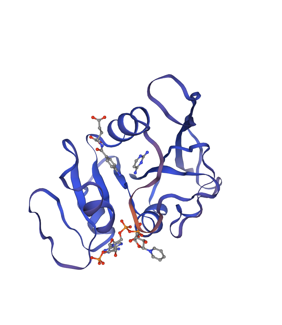
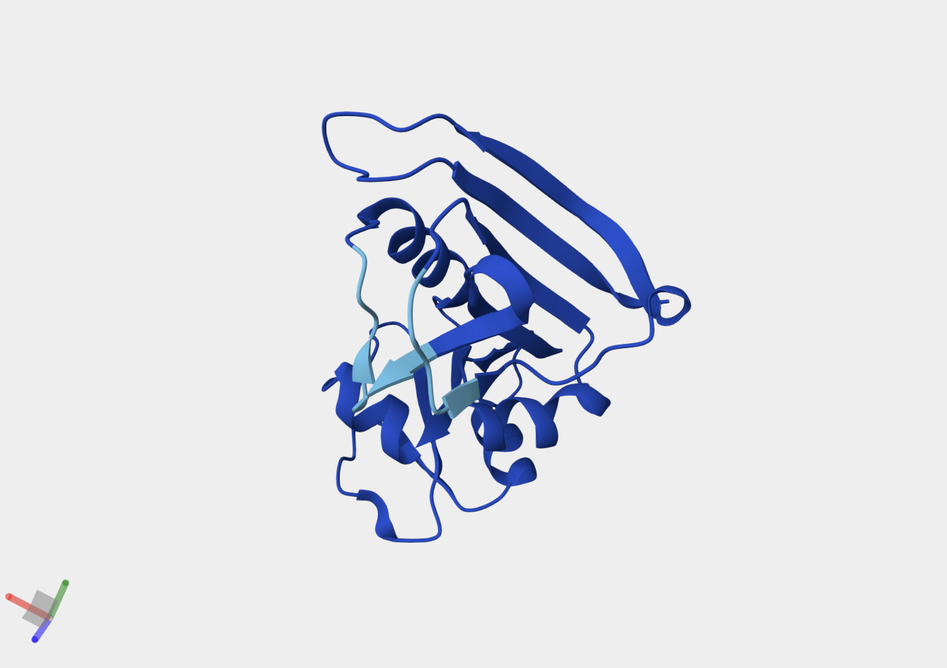

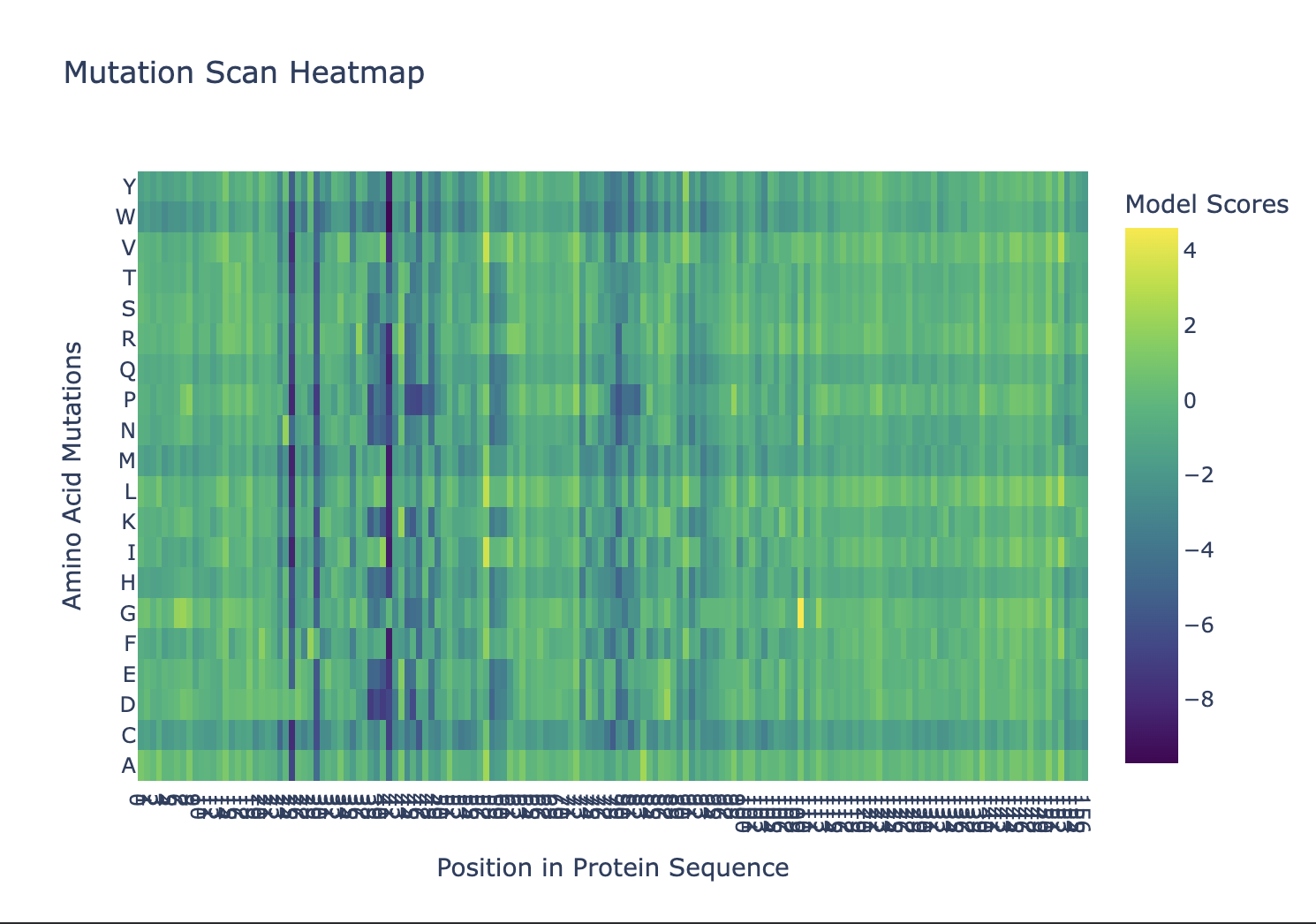
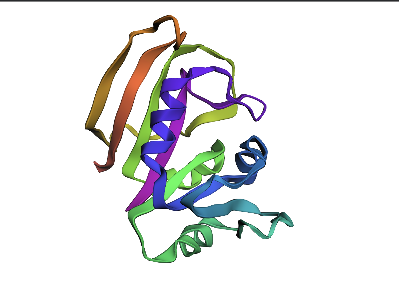
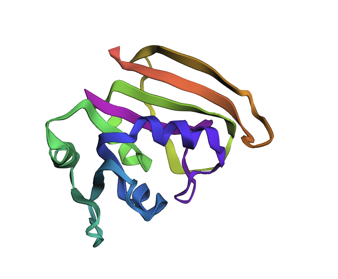
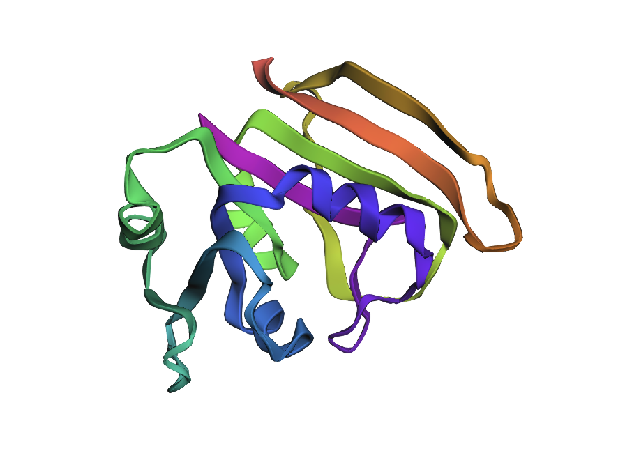
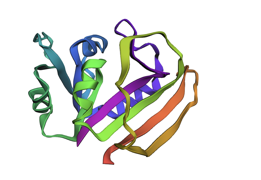
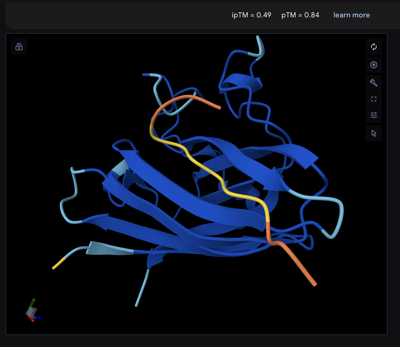
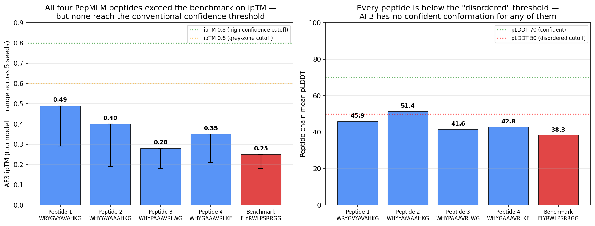
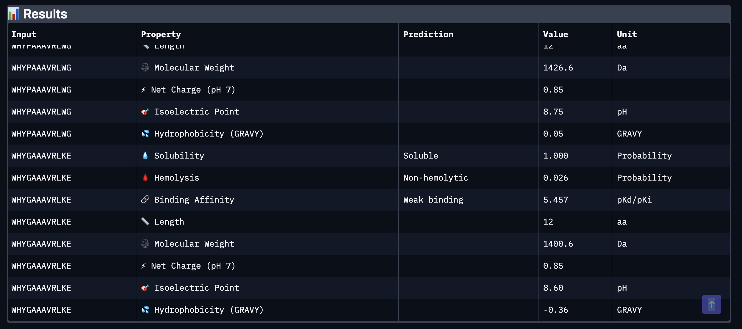
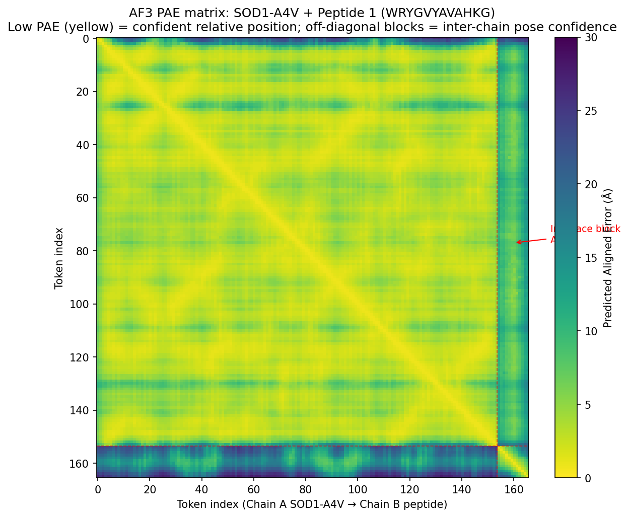
![moPPIt setup panel — De Novo mode, binder length 12, objectives [Solubility, Affinity, Motif] with equal weights, motif positions covering both target patches. The screenshot shows the initial <em>combined</em> motif setup before splitting into two separate runs (Run A = A4V cluster, Run B = dimer interface).](/2026a/fiona-connolly/homework/week-05-hw-protein-design-part-ii/img/04-moppit-setup-combined-motif.png)
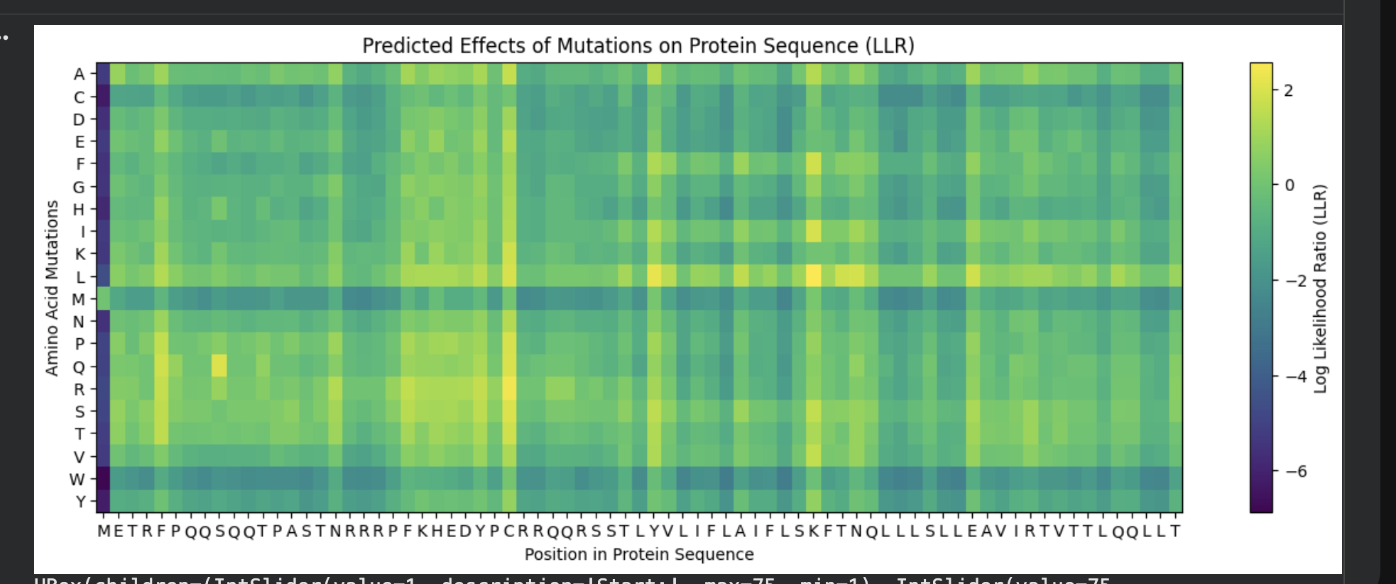
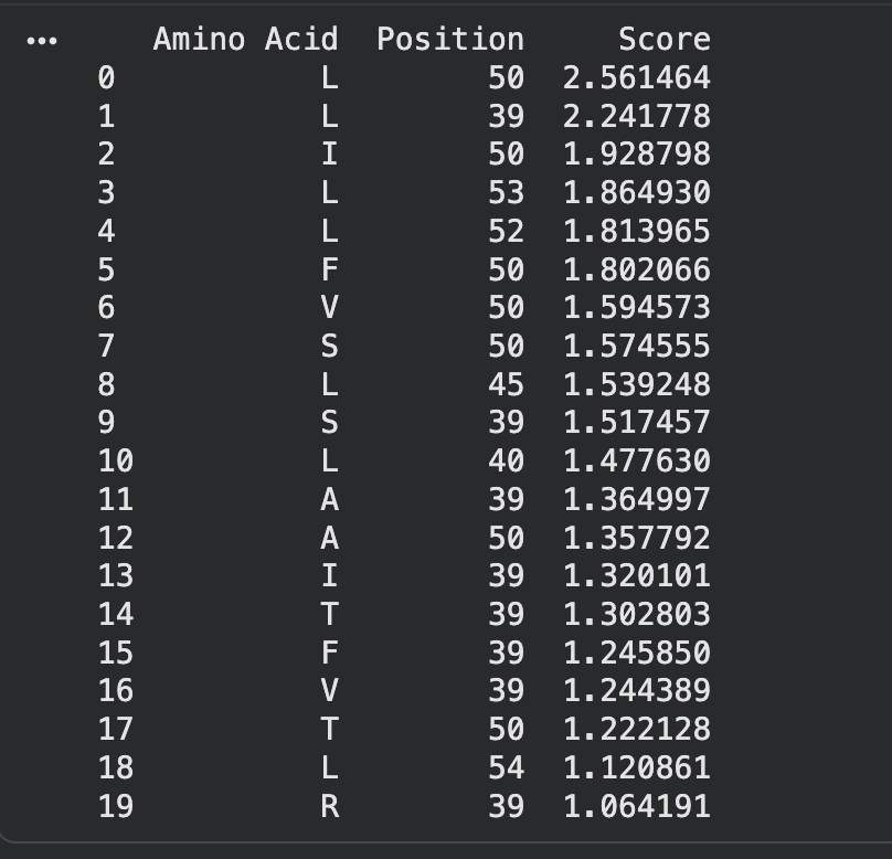
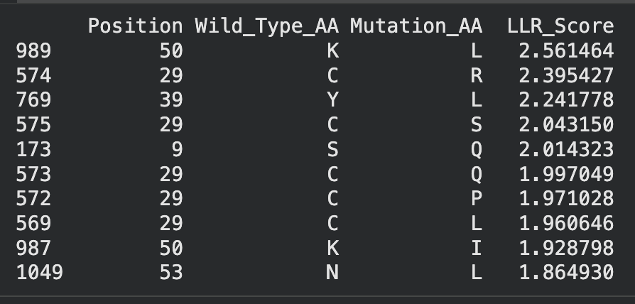
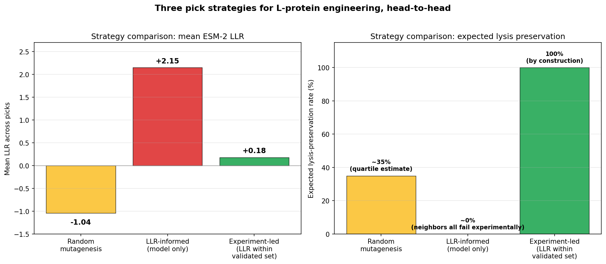
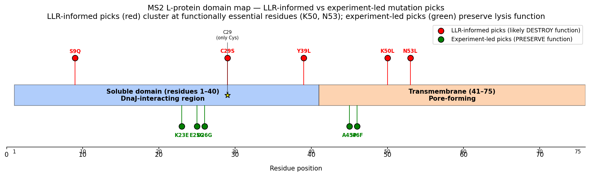
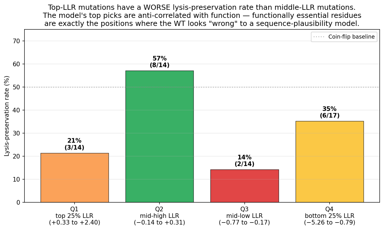
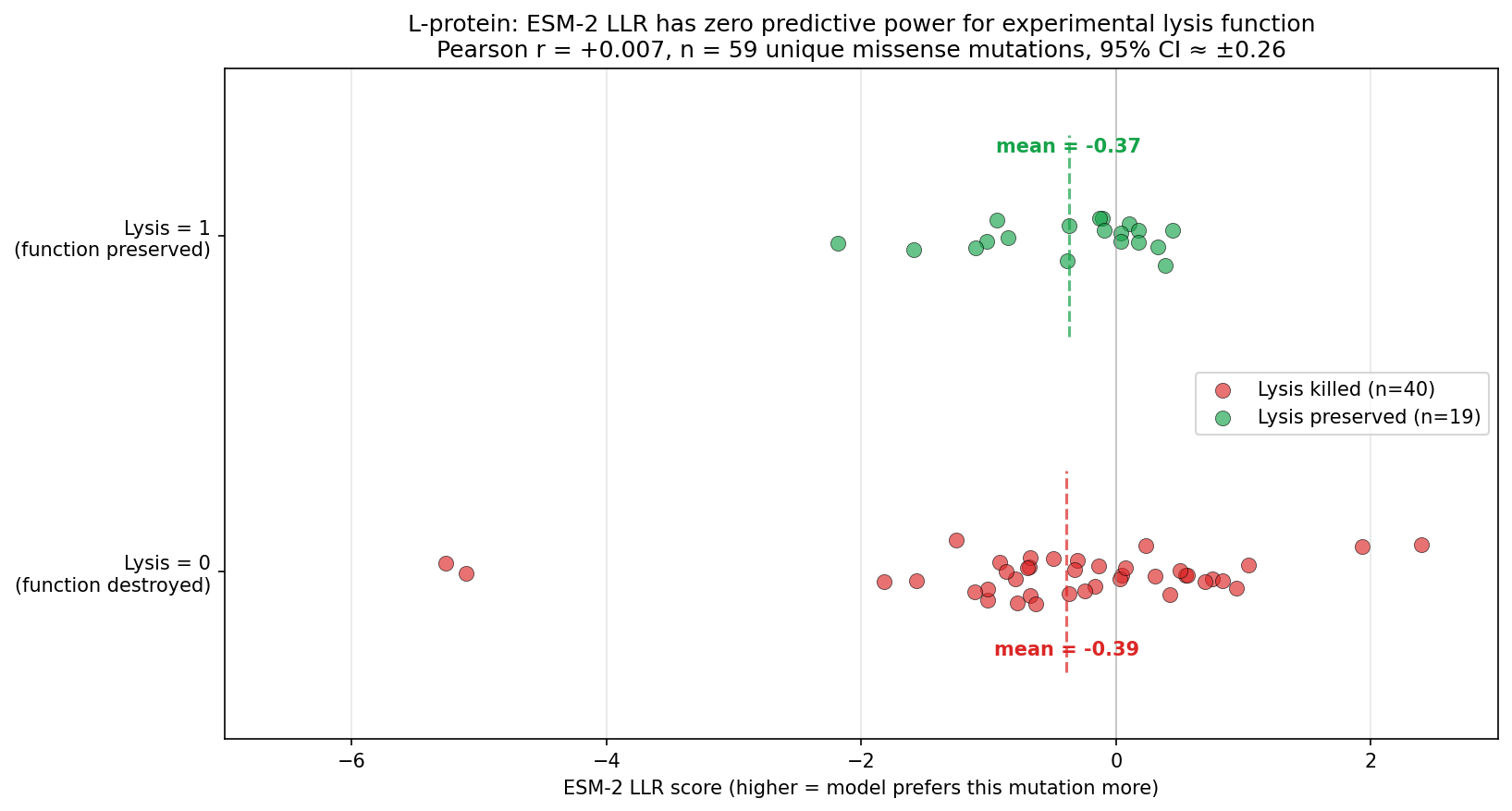
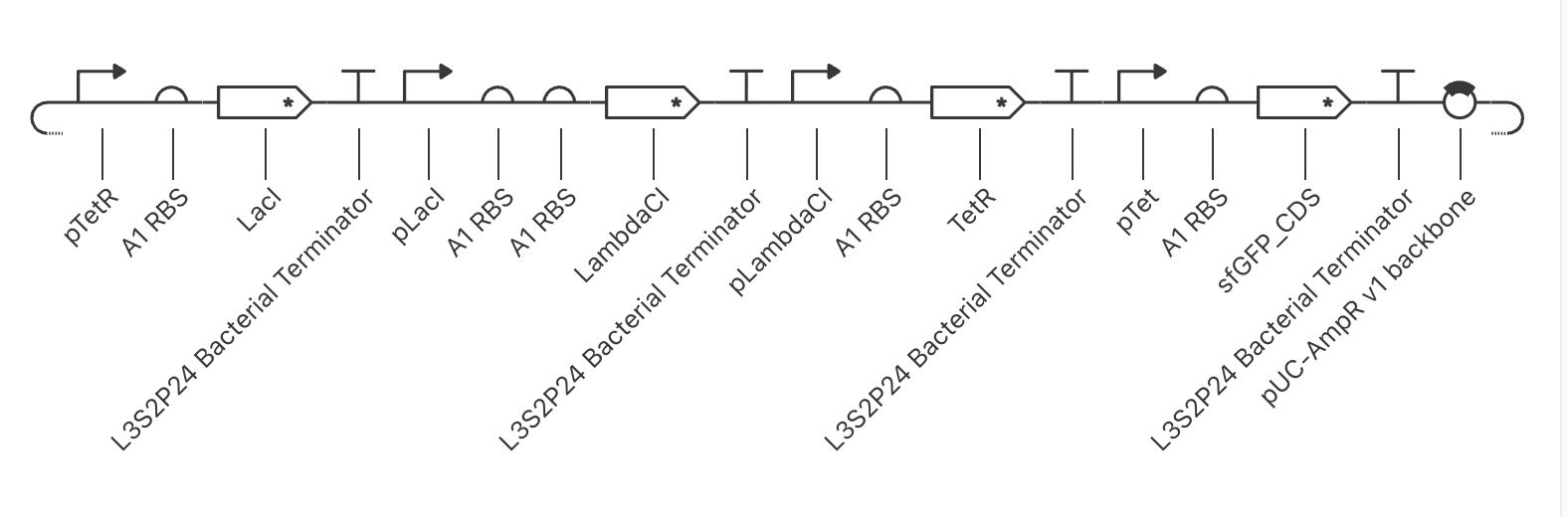
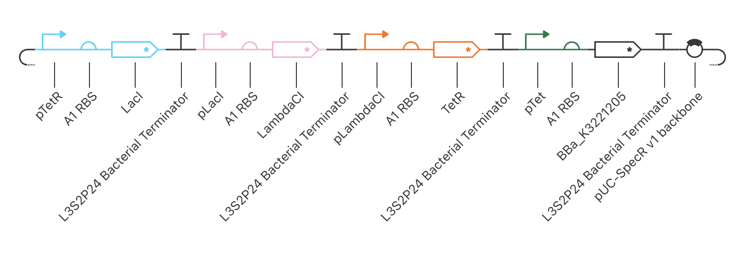
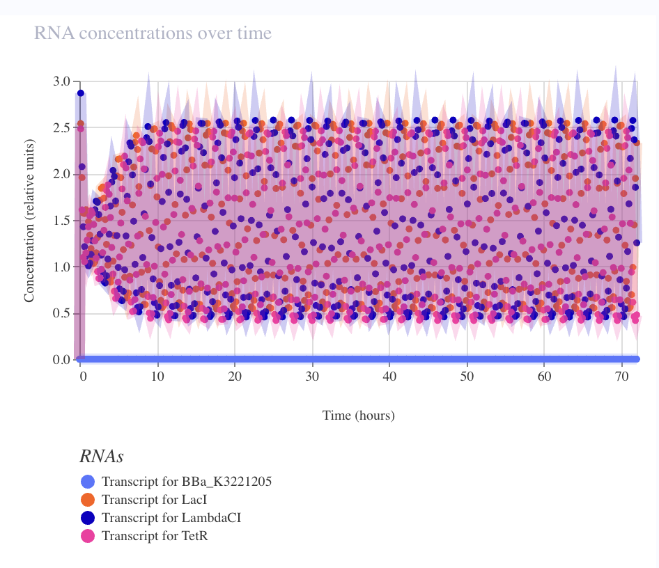
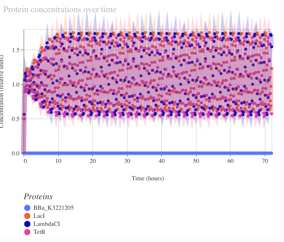
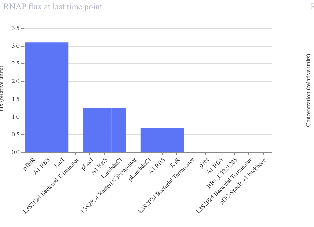
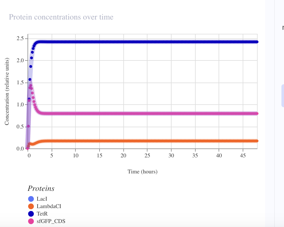
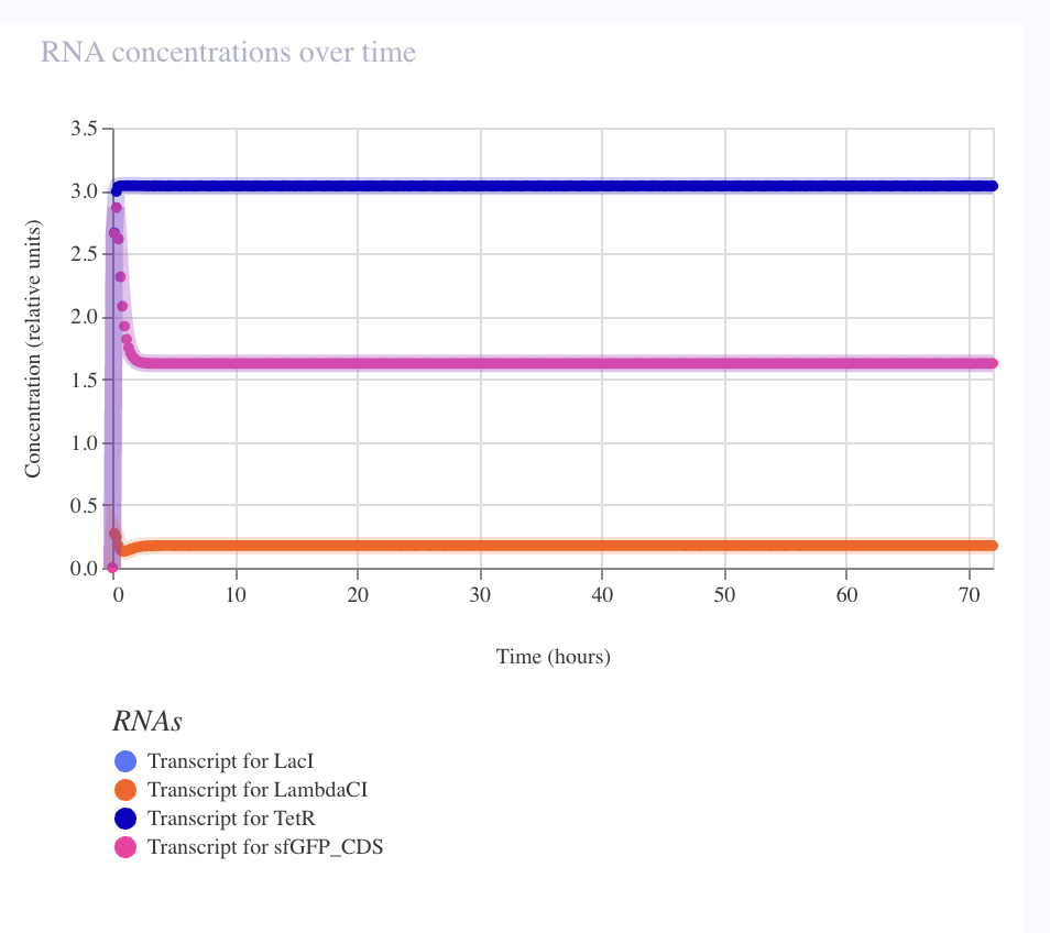
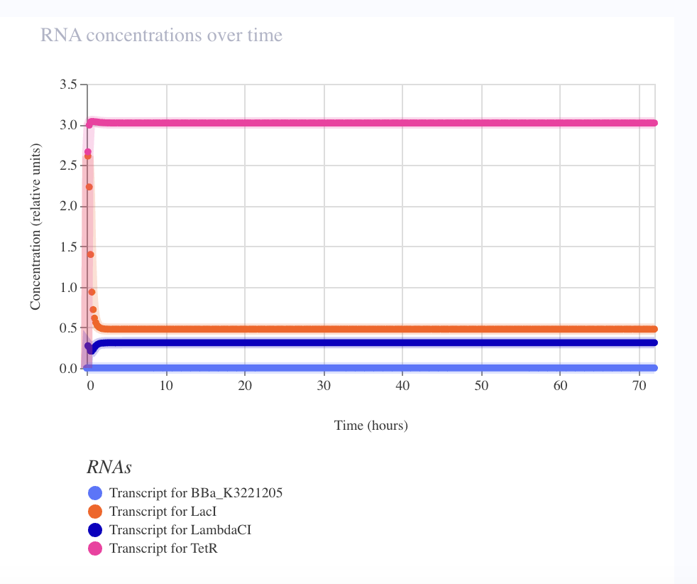
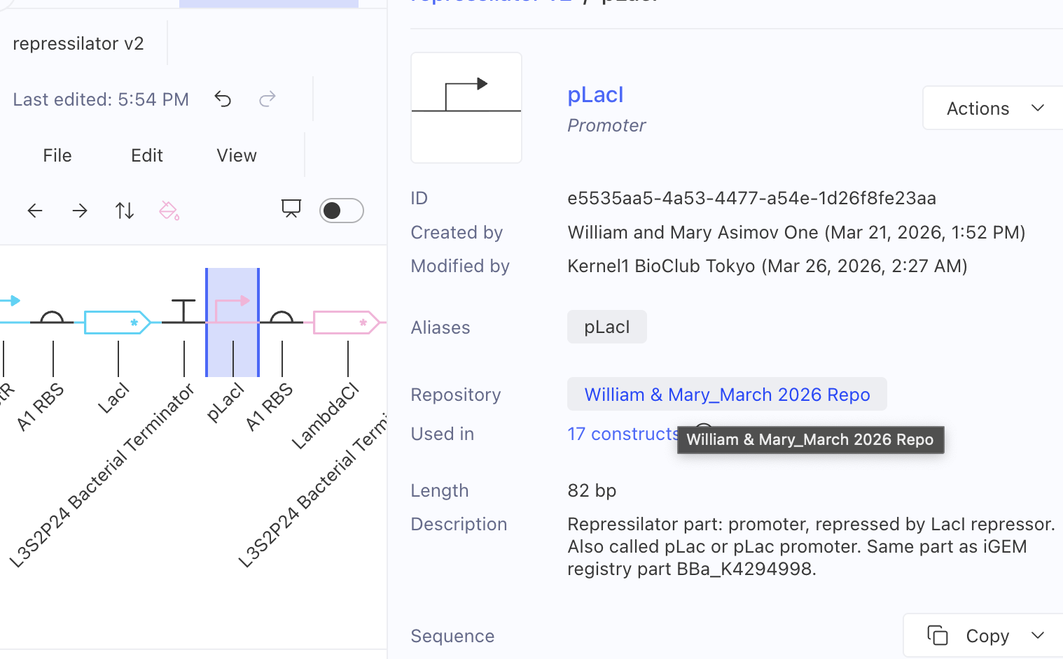
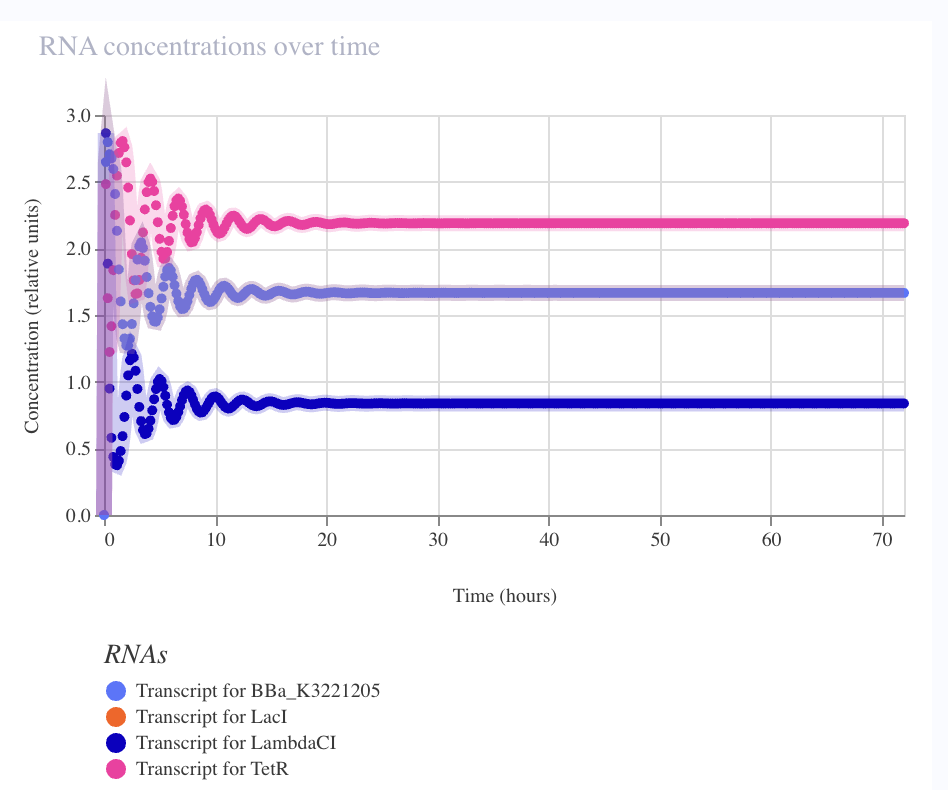
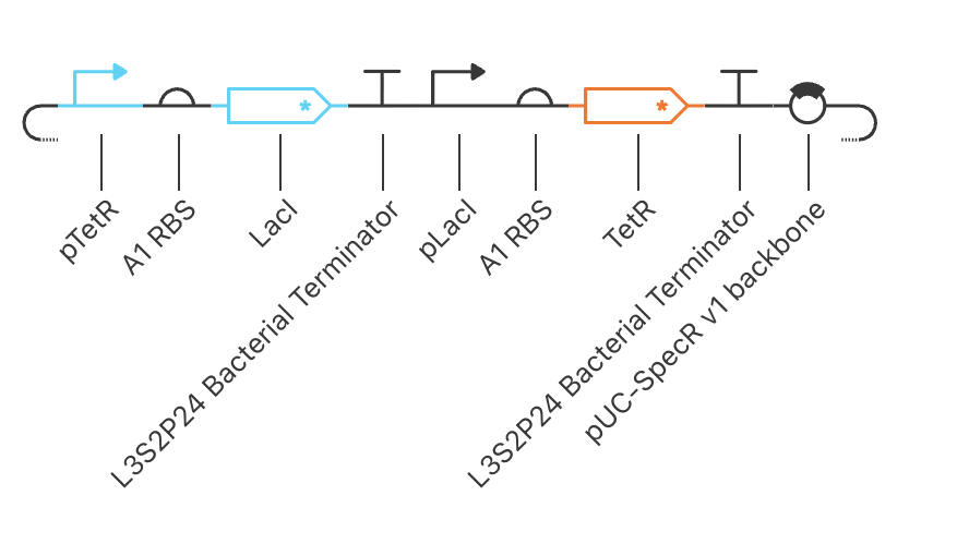
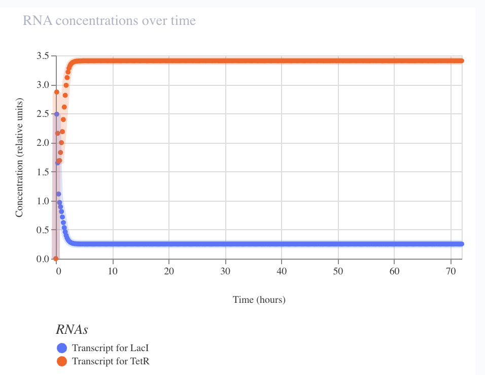
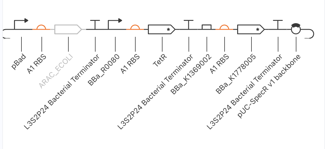
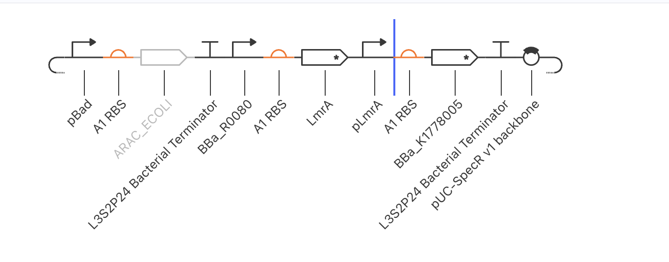
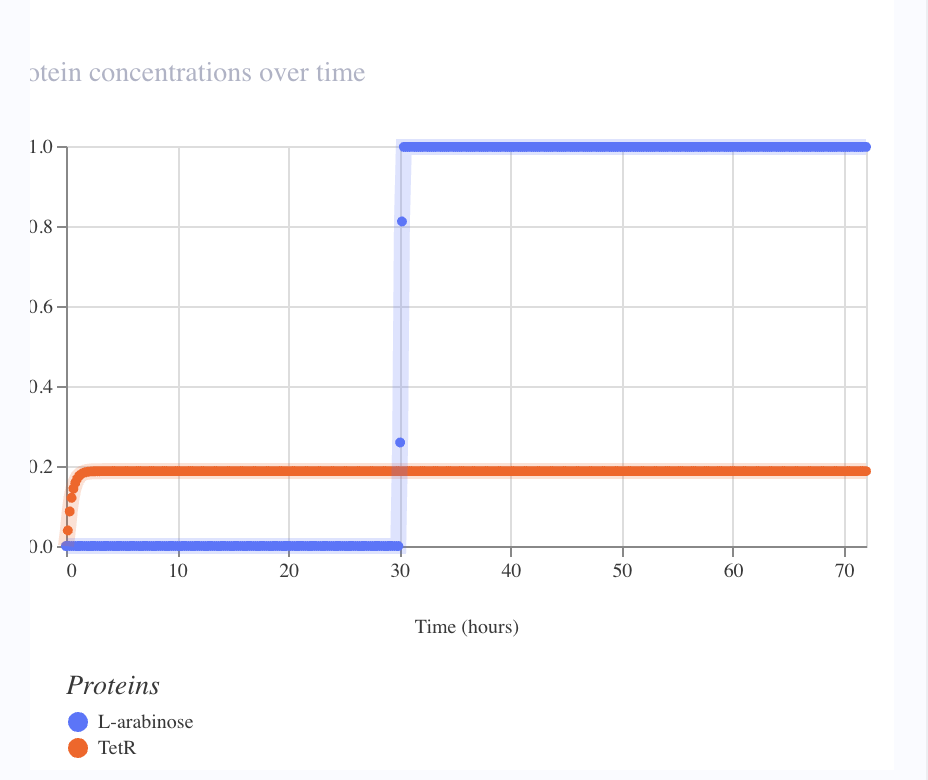
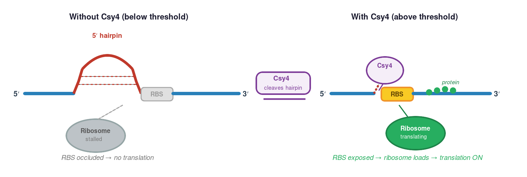
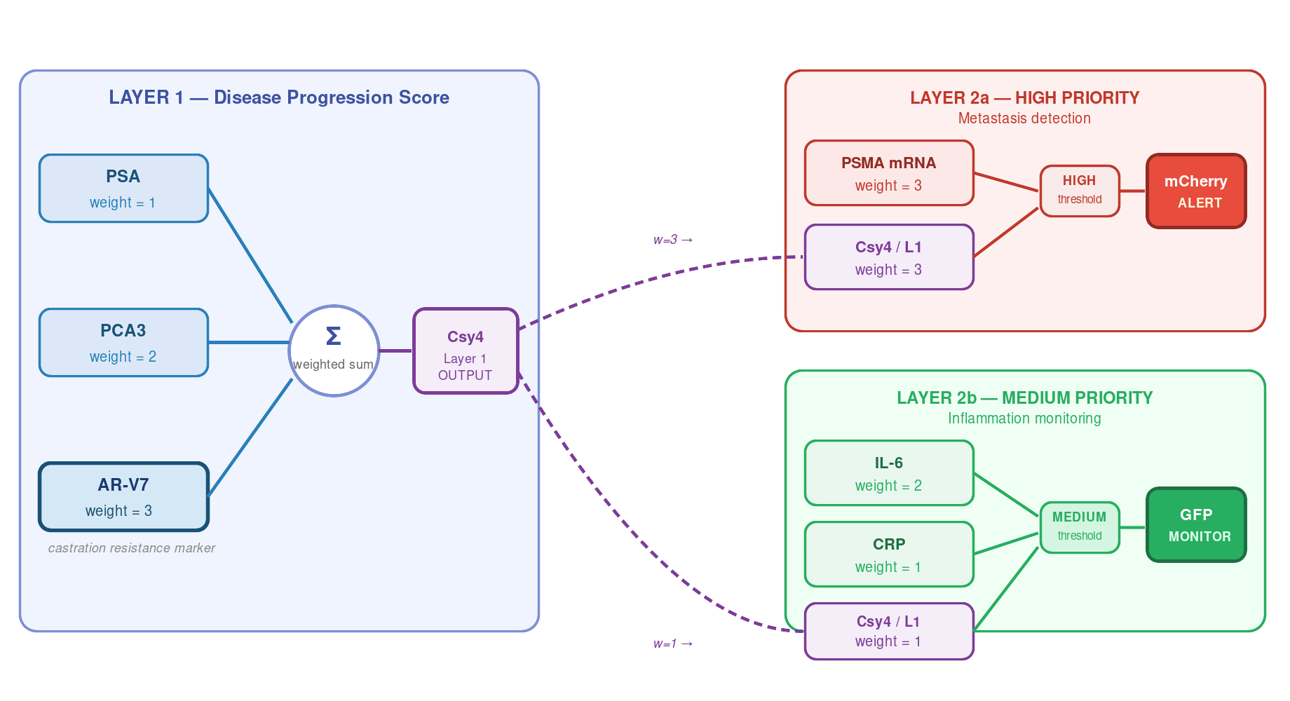

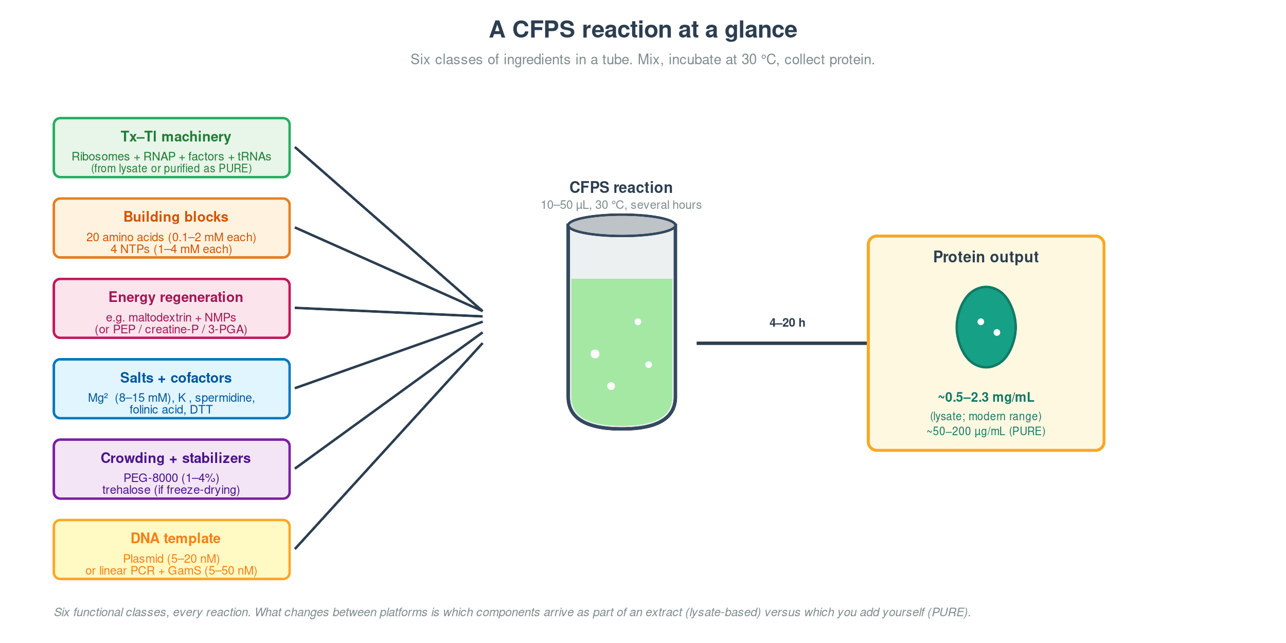
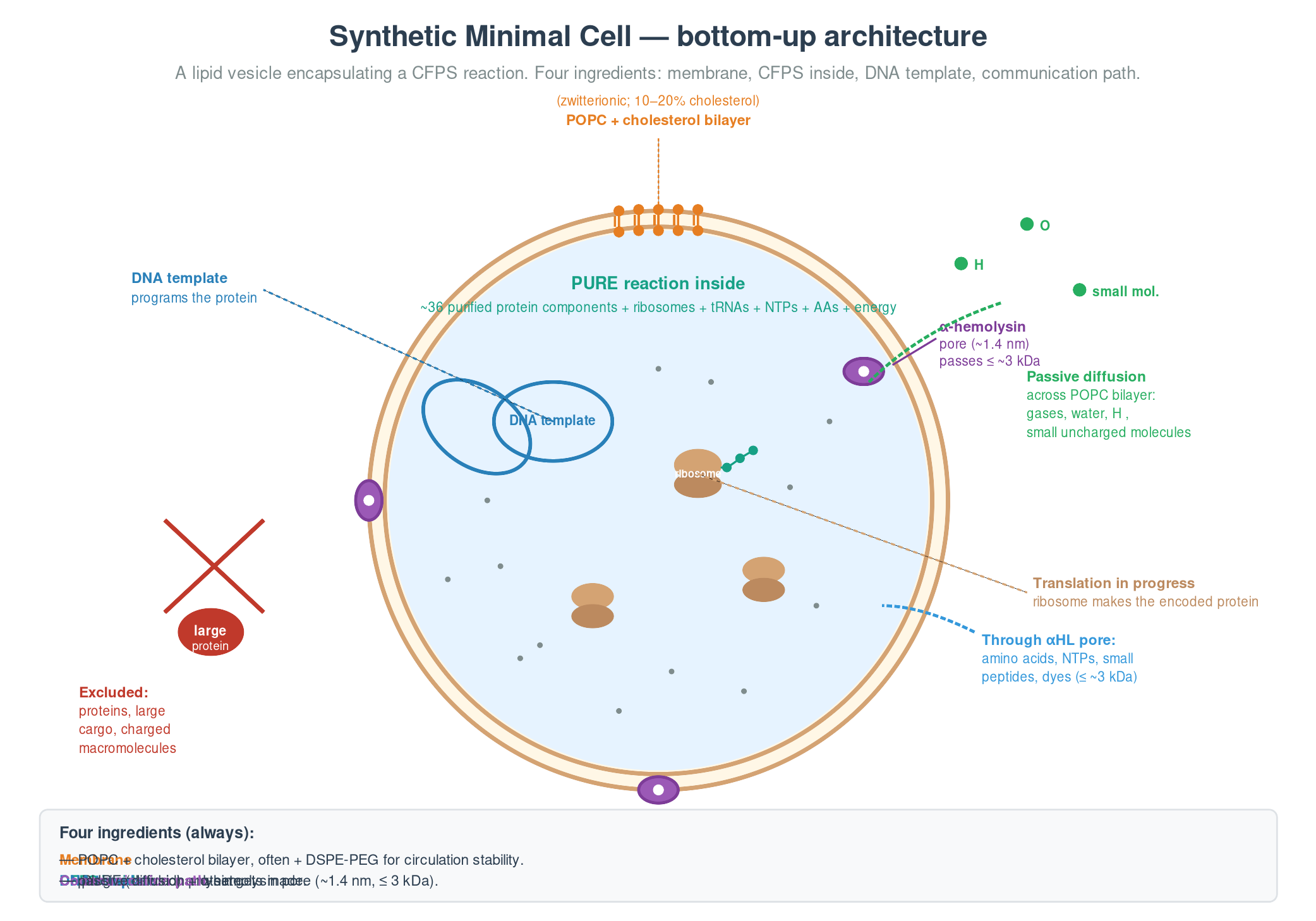
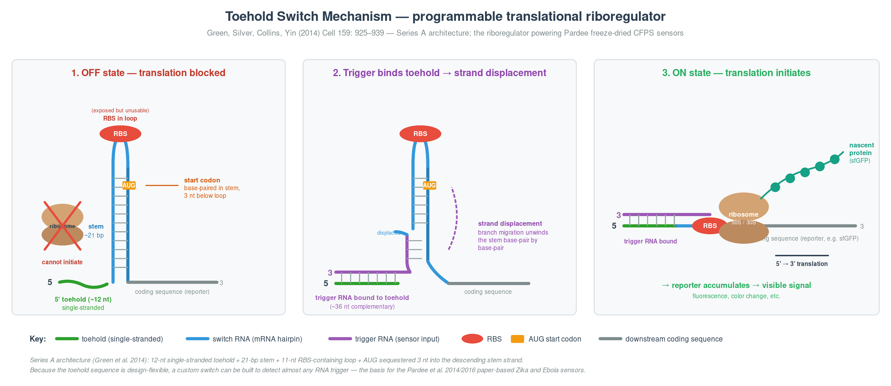
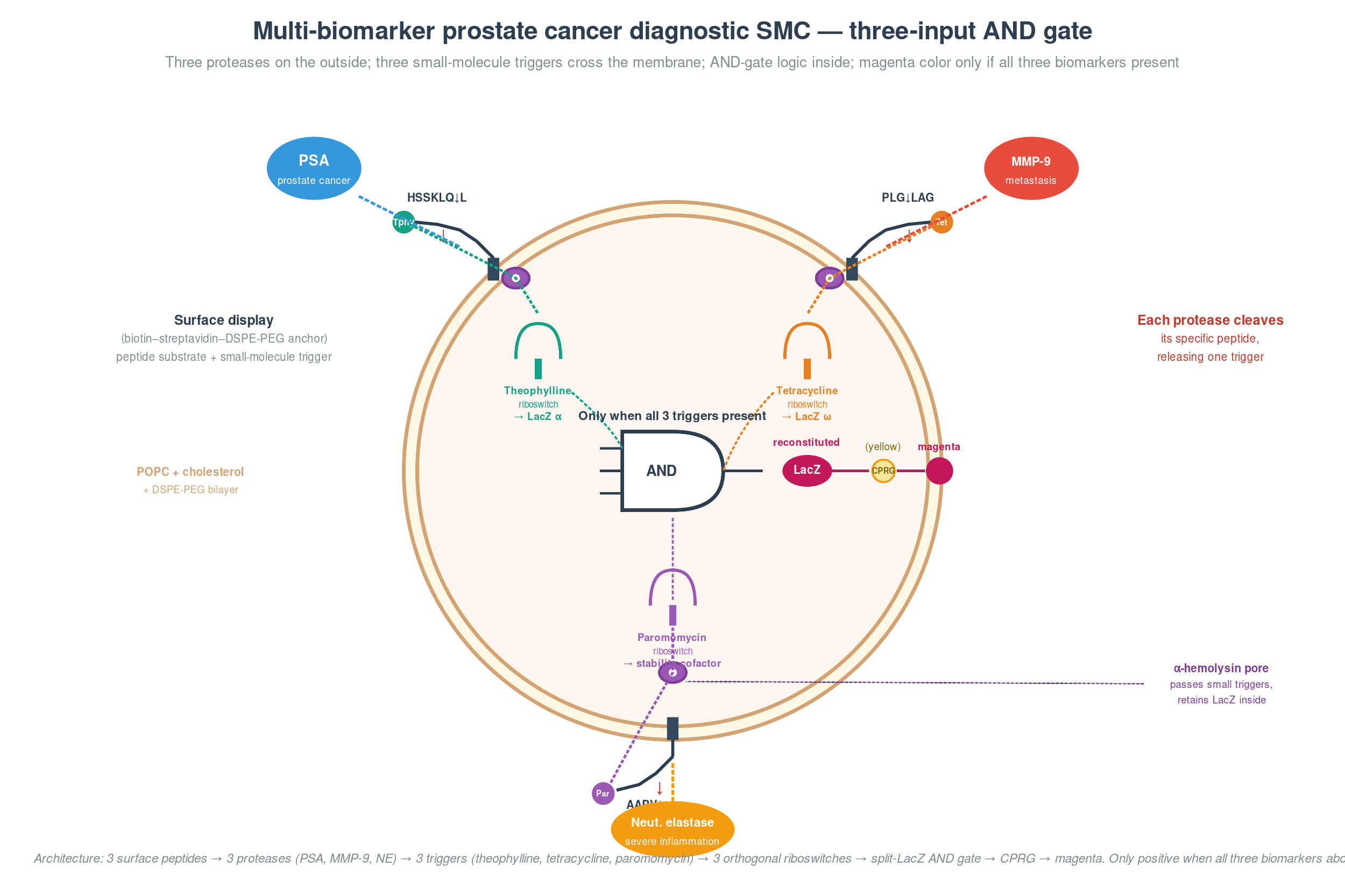


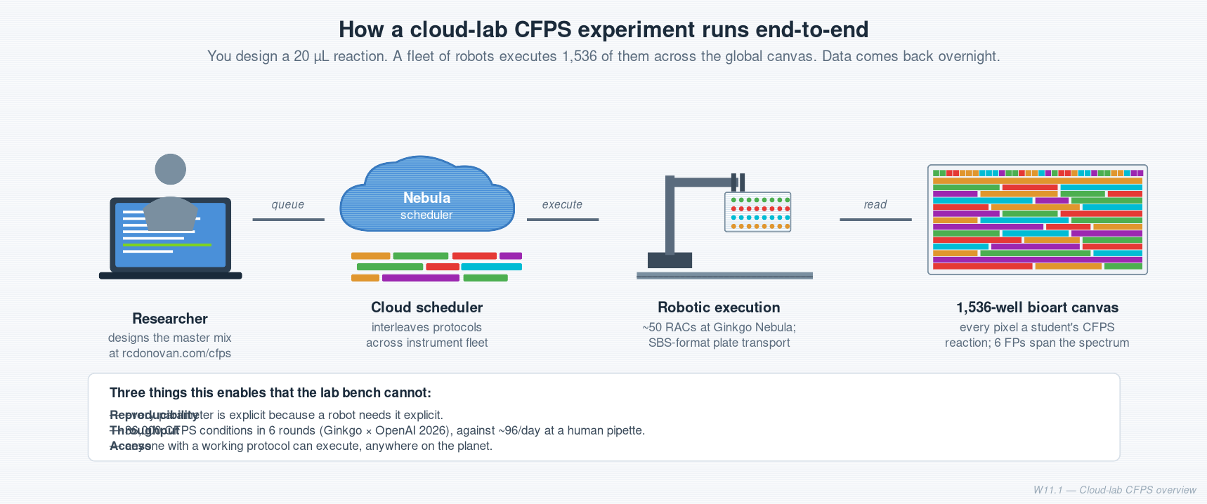
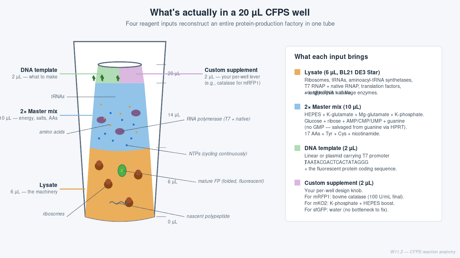
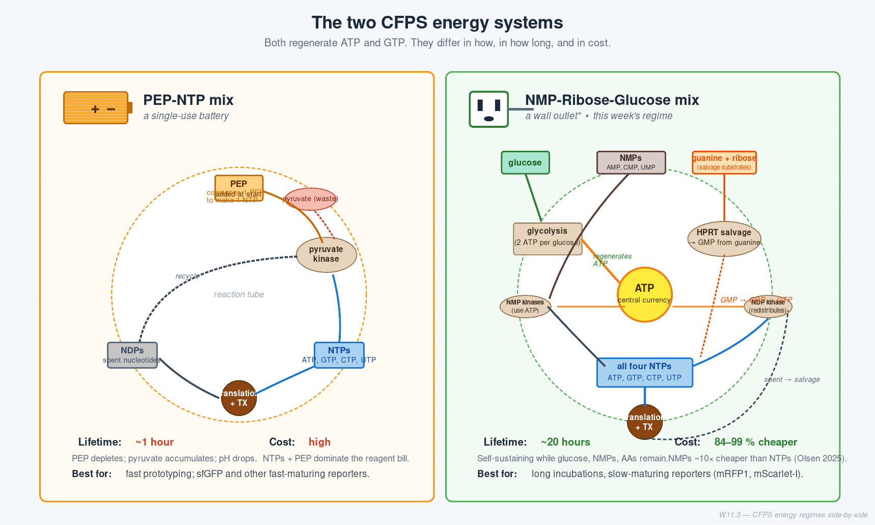
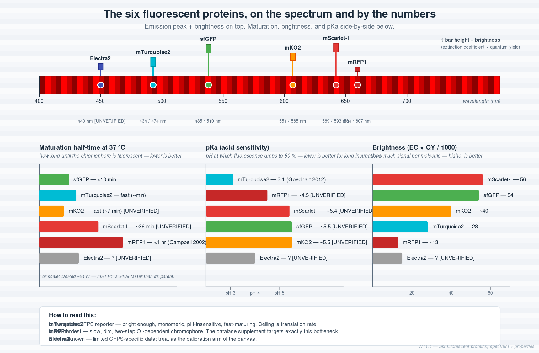


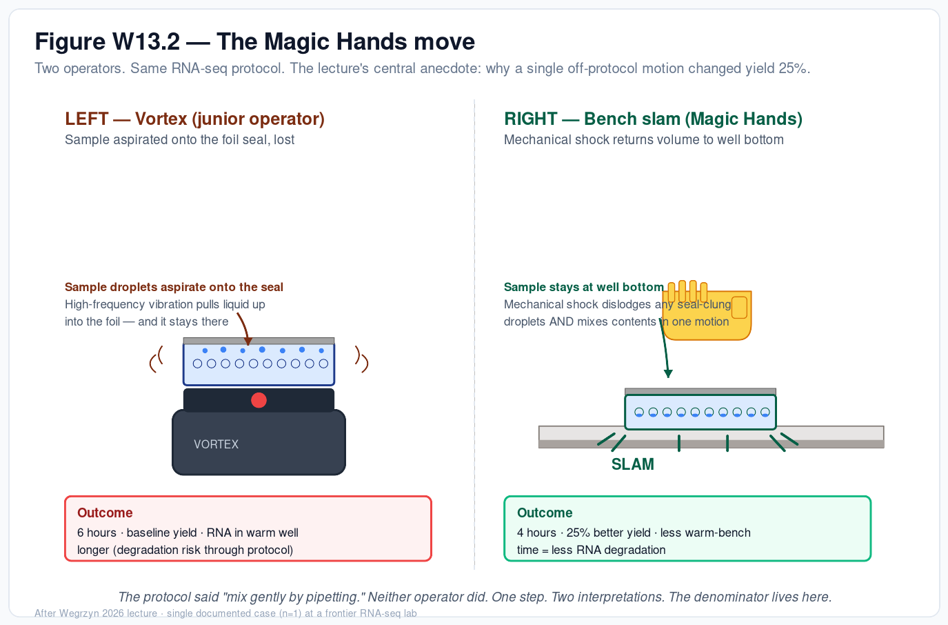
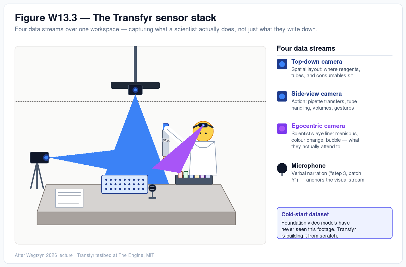
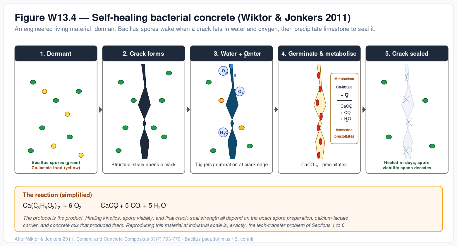
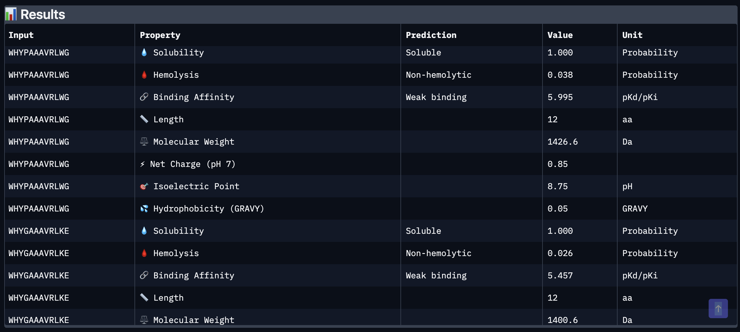