Week 10 HW: Advanced Imaging & Measurement Technology
Homework: Final Project
For your final project:
Please identify at least one (ideally many) aspect(s) of your project that you will measure. It could be the mass or sequence of a protein, the presence, absence, or quantity of a biomarker, etc.
For Aim 1 of my final project, there are several things I’ll need to measure, from confirming the construct is correct, to confirming the cells are expressing it, to ultimately quantifying the light output that defines success or failure of the experiment. The most important measurement is luminescence intensity from the IPTG-induced cells co-expressing nnLuz v4 truncated and nnH3H v2 after hispidin supplementation. This is the readout that directly tests my hypothesis that the v4 mutations stacked with the truncation produce a brighter enzyme pair than either modification alone. Light output alone isn’t enough without knowing the cells are actually doing what I think they’re doing, so I’ll also measure cell density (OD600) and perform a colony PCR to confirm the insert is present in transformed colonies.
Please describe all of the elements you would like to measure, and furthermore describe how you will perform these measurements.
First, I will confirm that transformed colonies contain the expected plasmid insert using colony PCR, followed by sequence verification if available. This checks that the DNA construct is present before moving into functional testing. Second, I will measure cell density using OD600 so that luminescence can be normalized to the amount of bacteria present rather than comparing raw light output from cultures with different growth levels. Third, I will measure bioluminescence intensity after IPTG induction and hispidin supplementation. This would be performed by imaging induced cultures in the dark using a sensitive camera or plate reader/luminometer if available. The signal could be quantified as relative light units or image intensity values, then normalized to OD600. Finally, I would compare induced versus uninduced cells, cells with and without hispidin, and any available control constructs. Together, these measurements would show whether the construct is present, whether the cells are growing comparably, and whether the engineered nnLuz v4 truncated / nnH3H v2 system produces detectable light.
What are the technologies you will use (e.g., gel electrophoresis, DNA sequencing, mass spectrometry, etc.)? Describe in detail.
The measurements I described in the previous question rely on a handful of standard molecular biology and analytical technologies. Here’s a detailed walkthrough of each one.
- PCR: PCR will be used for confirming whether transformed E. coli colonies actually carry my insert before I commit time to growing them up for expression. The reaction works by using a thermostable DNA polymerase (NEB OneTaq 2X Master Mix in my case) along with a pair of primers that flank the insert region of pET-28a(+). Through repeated cycles of denaturation (~95 °C), annealing (~55 °C), and extension (~68 °C), the target region between the primers is amplified exponentially. Turning a tiny amount of template DNA from a single colony into enough product to visualize. For colony PCR specifically, the template is just a small amount of bacteria picked from a plate and resuspended in water; the initial denaturation step lyses the cells and releases the plasmid. This is fast, cheap, and scales easily to screening 8–16 colonies in parallel, which is exactly what I need at this stage.
- Agarose Gel Electrophoresis: Once the colony PCR is done, I need a way to actually see whether the reaction produced a band of the expected size. Agarose gel electrophoresis works by casting a porous agarose gel (typically 1% for the size range I’m working with), loading PCR products into wells at one end, and applying an electric field across the gel. DNA is negatively charged, so it migrates toward the positive electrode, and the gel matrix acts as a sieve. Smaller fragments move faster and travel farther than larger ones. After running, the gel is stained with a DNA-binding dye (SYBR Safe or ethidium bromide) and visualized under UV or blue light. By running a DNA ladder of known sizes alongside my samples, I can confirm whether each colony’s PCR product matches the expected insert size. Colonies with the right band move forward; colonies with wrong-sized bands or no band get discarded.
- DNA Sequencing (Sanger): Colony PCR confirms something of the right size is there, but it can’t tell me whether the actual nucleotide sequence is correct. For that, I’ll use Sanger sequencing on the assembled plasmid. Sanger sequencing works by running a reaction that incorporates fluorescently labeled chain-terminating dideoxynucleotides (ddNTPs). Each time one is incorporated, the growing DNA strand stops, producing a population of fragments of every possible length, each tagged with a fluorescent base at its terminus. Capillary electrophoresis then separates these fragments by size, and a laser reads off the fluorescence color at each position, generating a chromatogram that gives the exact base-by-base sequence.
- UV-Vis Spectrophotometry: Measuring bacterial growth relies on the principle that a suspension of cells scatters light proportionally to the number of cells present. A spectrophotometer shines a beam of 600 nm light through a cuvette (or microplate well) containing the culture and measures how much light passes through versus how much is scattered or absorbed. The result, optical density at 600 nm (OD600), is a quick, non-destructive proxy for cell concentration. Six hundred nanometers is the standard wavelength because it’s long enough that E. coli cells don’t absorb it significantly through their natural pigments, so the reading reflects scattering (cell density) rather than chemistry. I’ll use this measurement at two key points: to determine when the culture has reached mid-log phase (OD600 ≈ 0.6) for IPTG induction, and at the time of luminescence measurement so I can normalize light output per cell.
- Plate Reader/Luminometer: This is the technology that produces the actual scientific readout of the experiment. A microplate reader in luminescence mode is essentially a very sensitive photon counter with a photomultiplier tube (PMT) positioned over each well of a 96-well plate. Unlike fluorescence (which requires an excitation light source), luminescence detection has no excitation step. The instrument just sits in the dark and counts photons emitted by the sample. This makes it ideal for autonomous bioluminescence, since the only light reaching the detector is light produced by the enzymatic reaction itself. I’ll use Greiner #655076 96-well black plates, where the opaque walls prevent light from one well bleeding into adjacent wells, which would otherwise contaminate measurements between different conditions. The reader integrates photon counts over a defined time window per well (typically 1 second) and outputs the result in relative light units (RLU).
Homework: Waters Part I — Molecular Weight
We will analyze an eGFP standard on a Waters Xevo G3 QTof MS system to determine the molecular weight of intact eGFP and observe its charge state distribution in the native and denatured (unfolded) states. The conditions for LC-MS analysis of intact protein cause it to unfold and be detected in its denatured form (due to the solvents and pH used for analysis).
- Based on the predicted amino acid sequence of eGFP (see below) and any known modifications, what is the calculated molecular weight?
eGFP Sequence:MVSKGEELFTG VVPILVELDG DVNGHKFSVS GEGEGDATYG KLTLKFICTT GKLPVPWPTL VTTLTYGVQC FSRYPDHMKQ HDFFKSAMPE GYVQERTIFF KDDGNYKTRA EVKFEGDTLV NRIELKGIDF KEDGNILGHK LEYNYNSHNV YIMADKQKNG IKVNFKIRHN IEDGSVQLAD HYQQNTPIGD GPVLLPDNHY LSTQSALSKD PNEKRDHMVL LEFVTAAGIT LGMDELYKLE HHHHHH
Note: This contains a His-purification tag (HHHHHH) and a linker (the LE before it).
- Calculated molecular weight: 28,006.60 Da
Calculate the molecular weight of the eGFP using the adjacent charge state approach described in the recitation. Select two charge states from the intact LC-MS data (Figure 1) and:
- Determine $z$ for each adjacent pair of peaks $(n, n+1)$ using: $$ {\large z} = {\Large \frac{\frac{m}{z_{n+1}}}{\frac{m}{z_n} - \frac{m}{z_{n+1}}}} $$ $$ z = \frac{1400.46}{1474.11 - 1400.46} $$ $$ z = \frac{1400.46}{73.65} \approx 19 $$
- Determine the MW of the protein using the relationship between $\frac{m}{z_n}$, $MW$, and $z$ $$ M = 19(1474.11) - 19(1.0073) = 27,989 \text{Da} $$
- Calculate the accuracy of the measurement using the deconvoluted MW from 2.2 and the predicted weight of the protein from 2.1 using: $$ \text{Accuracy} = \frac{|MW_{\text{experiment}} - MW_{\text{theory}}|}{MW_{\text{theory}}} $$ $$ \text{Accuracy} = \frac{|27989 - 28006.60|}{28006.60} $$ $$ \text{Accuracy} = 0.000628 \approx 0.0628\text{%} $$
Can you observe the charge state for the zoomed-in peak in the mass spectrum for the intact eGFP? If yes, what is it? If no, why not?
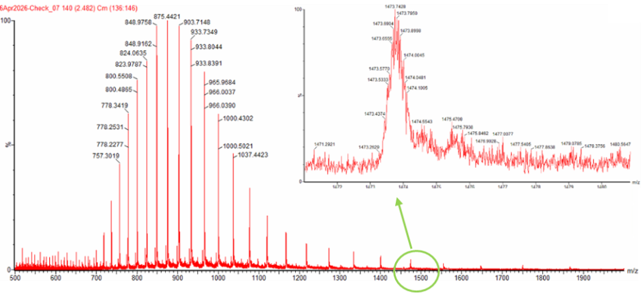
Figure 1. Mass Spectrum of intact eGFP protein from the Waters Xevo G3 LC-MS (a mass spectrometer with 30,000 resolution) with individual charge state peaks labeled with $\frac{m}{z}$ values.
No, the charge state cannot be directly observed from the zoomed-in peak alone because the isotopic peaks are not sufficiently resolved to measure the spacing between them.
Homework: Waters Part II — Secondary/Tertiary structure
We will analyze eGFP in its native, folded state and compare it to its denatured, unfolded state on a quadrupole time-of-flight MS. We will be doing MS-only analysis (no liquid chromatography, also known as “direct infusion” experiments) on the Waters Xevo G3-QToF MS.
- Based on learnings in the lab, please explain the difference between native and denatured protein conformations. For example, what happens when a protein unfolds? How is that determined with a mass spectrometer? What changes do you see in the mass spectrum between the native and denatured protein analyses (Figure 2)?
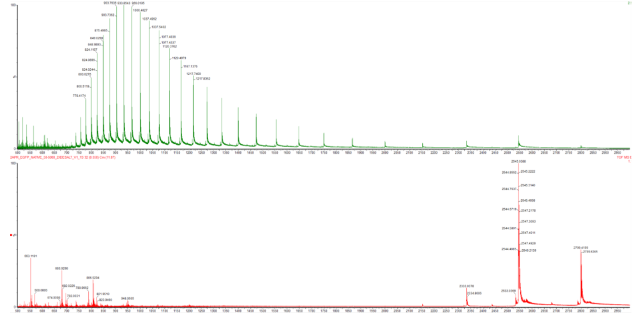
Figure 2. Comparison of the mass spectra between denatured (top) and native (bottom) eGFP standard on the Waters Xevo G3 QTof MS.
In the native conformation, the protein is folded into a compact structure, which buries many protonatable residues such as lysine, arginine, and histidine. As a result, fewer protons can be added during ionization, leading to lower charge states and peaks at higher $\frac{m}{z}$ values. In contrast, when the protein denatures, it unfolds and exposes these residues to the solvent, allowing more protons to attach. This results in higher charge states and peaks at lower $\frac{m}{z}$ values.
Mass spectrometry detects this difference indirectly through the charge state distribution. In the denatured spectrum (Figure 2, top), there is a broad distribution of peaks at lower $\frac{m}{z}$ values, indicating many high charge states. In the native spectrum (Figure 2, bottom), the peaks are fewer and shifted to higher $\frac{m}{z}$ values, indicating lower charge states. This shift in charge state distribution reflects the transition from a folded to an unfolded protein conformation.
- Zooming into the native mass spectrum of eGFP from the Waters Xevo G3 QTof MS (see Figure 3), can you discern the charge state of the peak at ~2800 $\frac{m}{z}$? What is the charge state? How can you tell?
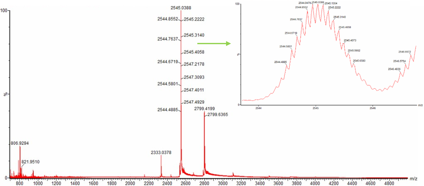
Figure 3. Native eGFP mass spectrum from the Waters Xevo G3 Q-Tof MS. The inset is a zoomed-in view of the charge state at ~2800 $\frac{m}{z}$ on a mass spectrometer with 30,000 resolution.
Yes, the charge state can be determined from the zoomed-in peak by measuring the spacing between adjacent isotopic peaks. The spacing between peaks is approximately 0.092 $\frac{m}{z}$. Since isotope spacing follows Δ($\frac{m}{z}$) = $\frac{1}{z}$, the charge state can be calculated as z ≈ $\frac{1}{0.092}$ ≈ 11. Therefore, the peak at ~2800 $\frac{m}{z}$ corresponds to a charge state of approximately 11+.
Homework: Waters Part III — Peptide Mapping - primary structure
We will digest the eGFP protein standard into peptides using trypsin (an enzyme that selectively cleaves the peptide bond after Lysine (K) and Arginine (R) residues. The resulting peptides will be analyzed on the Waters BioAccord LC-MS to measure their molecular weights and fragmented to confirm the amino acid sequence within each peptide – generating a “peptide map”. This process is used to confirm the primary structure of the protein.
There are a variety of tools available online to calculate protein molecular weight and predict a list of peptides generated from a tryptic digest. We will be using tools within the online resource Expasy (the bioinformatics resource portal of the Swiss Institute of Bioinformatics (SIB)) to predict a list of tryptic peptides from eGFP.
- How many Lysines (K) and Arginines (R) are in eGFP? Please circle or highlight them in the eGFP sequence given in Waters Part I question 1 above. (Note: adding the sequence to Benchling as an amino acid file and clicking biochemical properties tab will show you a count for each amino acid).
- Lysines = 20
- Arginines = 6
eGFP Sequence:
MVSKGEELFTG VVPILVELDG DVNGHKFSVS GEGEGDATYG KLTLKFICTT GKLPVPWPTL VTTLTYGVQC FSRYPDHMKQ HDFFKSAMPE GYVQERTIFF KDDGNYKTRA EVKFEGDTLV NRIELKGIDF KEDGNILGHK LEYNYNSHNV YIMADKQKNG IKVNFKIRHN IEDGSVQLAD HYQQNTPIGD GPVLLPDNHY LSTQSALSKD PNEKRDHMVL LEFVTAAGIT LGMDELYKLE HHHHHH
- How many peptides will be generated from tryptic digestion of eGFP?
- Navigate to https://web.expasy.org/peptide_mass/
- Copy/paste the sequence above into the input box in the PeptideMass tool to generate expected list of peptides.
- Use Figure 4 below as a guide for the relevant parameters to predict peptides from eGFP.
- Click “Perform the Cleavage” button in the PeptideMass tool and report the number of peptides generated when using trypsin to perform the digest.
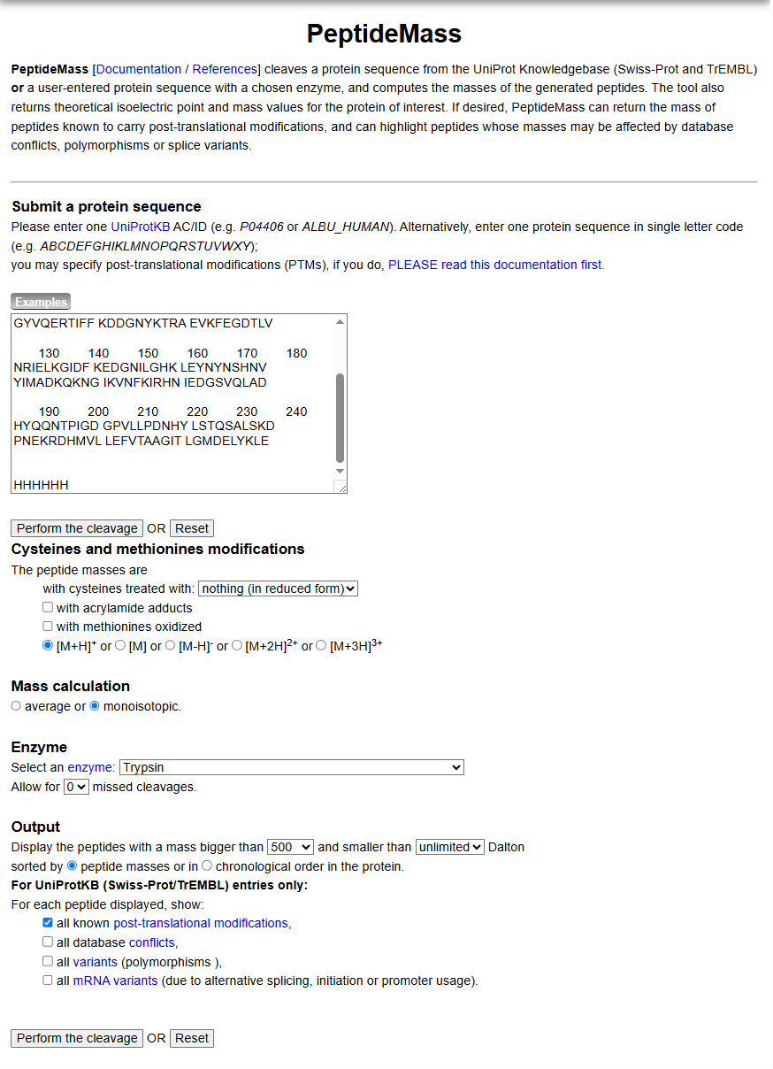
Figure 4. Example conditions for predicting the number of tryptic peptides from the eGFP standard. Please replicate all parameters shown above.
- Peptides generated = 19
- Based on the LC-MS data for the Peptide Map data generated in lab (please use Figure 5a as a reference) how many chromatographic peaks do you see in the eGFP peptide map between 0.5 and 6 minutes? You may count all peaks that are >10% relative abundance.
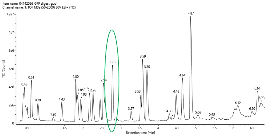
Figure 5a. Total ion chromatogram (TIC) of the eGFP peptide map. The peak at 2.78 minutes is circled, and its MS data is shown in the mass spectrum in Figure 5b, below.
- Chromatographic Peaks = 16
- Assuming all the peaks are peptides, does the number of peaks match the number of peptides predicted from question 2 above? Are there more peaks in the chromatogram or fewer?
- The number of peaks does not match the number of peptides predicted from question 2. There are fewer peaks in the chromatogram.
- Identify the mass-to-charge ($\frac{m}{z}$) of the peptide shown in Figure 5b. What is the charge ($z$) of the most abundant charge state of the peptide (use the separation of the isotopes to determine the charge state). Calculate the mass of the singly charged form of the peptide ($\small{[M\!\!+\!\!H]^+}$) based on its $\frac{m}{z}$ and $z$.
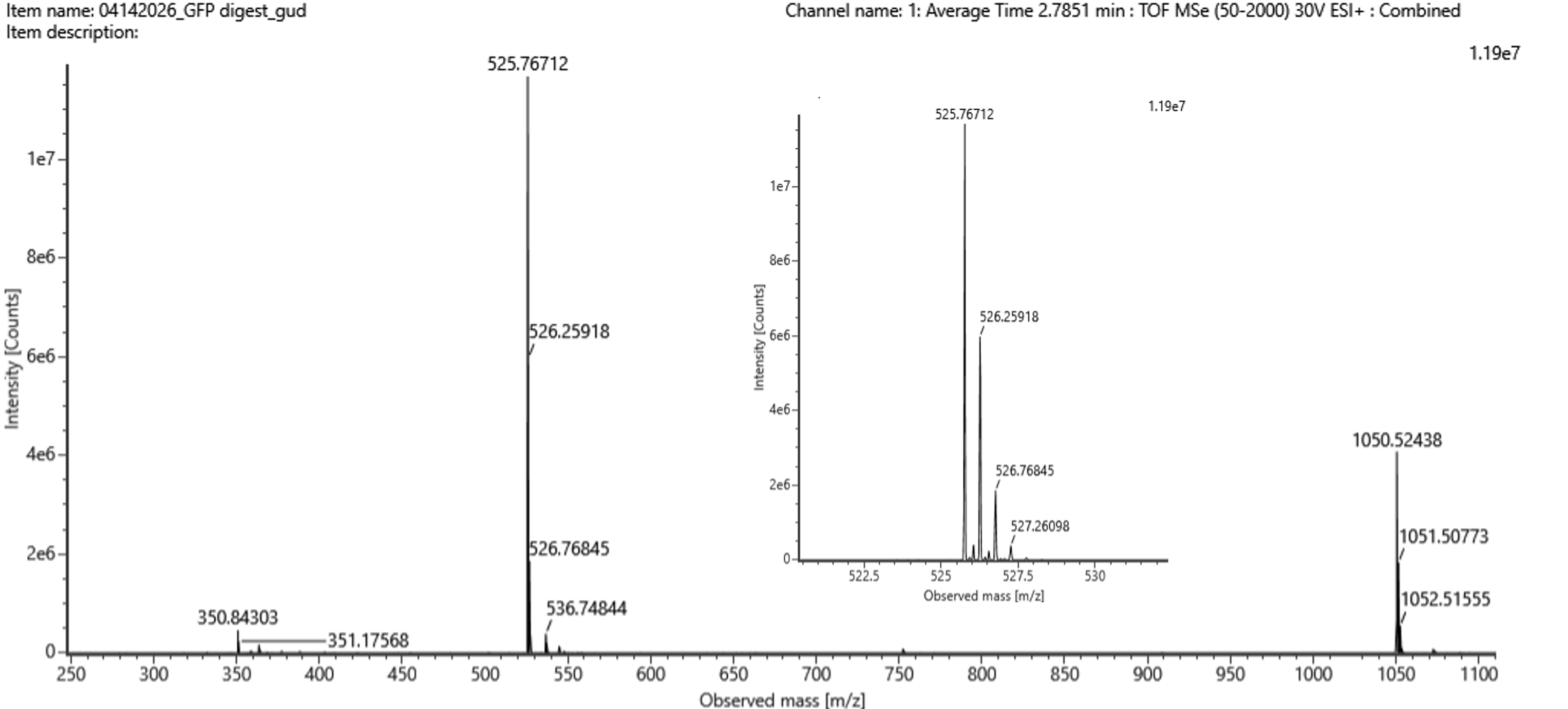
Figure 5b. Mass spectrum figure to show $\frac{m}{z}$ for the chromatographic peak at 2.78 min from Figure 5a above. The inset is a zoom-in of the peak at $\frac{m}{z}$ 525.76, to discern the isotope peaks.
- The most abundant peptide peak is observed at $\frac{m}{z}$ 525.76712. The isotope spacing is approximately 0.5 $\frac{m}{z}$, so using Δ($\frac{m}{z}$) = $\frac{1}{z}$, the charge state is 2+. The mass of the singly charged form is calculated as: $$ (\small{[M\!\!+\!\!H]^+}) = 2(525.76712) - 1.0073 = 1050.52694 $$
- Therefore, the singly charged peptide has a mass of approximately 1050.53 $\frac{m}{z}$.
- Identify the peptide based on comparison to expected masses in the PeptideMass tool. What is mass accuracy of measurement? Please calculate the error in ppm. (Recall that $ \text{Accuracy} = \frac{|MW_{\text{experiment}} - MW_{\text{theory}}|}{MW_{\text{theory}}} $ )
- The peptide is FEGDTLVNR because its theoretical ($\small{[M\!\!+\!\!H]^+}$) mass in the PeptideMass table is 1050.5214, which matches the observed peptide mass. Using the observed singly charged peak at 1050.52438, the mass error is:
$$ \text{ppm error} = (\frac{|1050.52438 - 1050.5214|}{1050.5214}) × 10^6 = 2.84 \text{ppm} $$
- Therefore, the peptide is identified as FEGDTLVNR with a mass accuracy of 2.84 ppm.
- What is the percentage of the sequence that is confirmed by peptide mapping? (see Figure 6)
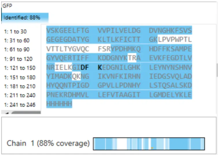
Figure 6. Amino Acid Coverage Map of eGFP based on BioAccord LC-MS peptide identification data.
- The percentage of the sequence confirmed by peptide mapping is 88%, as indicated by the sequence coverage shown in Figure 6.
Homework: Waters Part IV — Oligomers
We will determine Keyhole Limpet Hemocyanin (KLH)’s oligomeric states using charge detection mass spectrometry (CDMS). CDMS single-particle measurements of KLH allow us to make direct mass measurements to determine what oligomeric states (that is, how many protein subunits combine) are present in solution. Using the known masses of the polypeptide subunits (Table 1) for KLH, identify where the following oligomeric species are on the spectrum shown below from the CDMS (Figure 7):
- 7FU Decamer
- 8FU Didecamer
- 8FU 3-Decamer
- 8FU 4-Decamer
| Polypeptide Subunit Name | Subunit Mass |
|---|---|
| 7FU | 340 kDa |
| 8FU | 400 kDa |
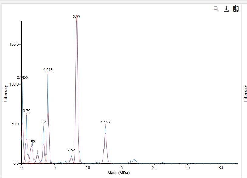
Figure 7. Mass spectrum of Keyhole Limpet Hemocyanin (KLH) acquired on the CDMS.
- The oligomeric species are identified by multiplying the subunit mass by the number of subunits in the assembly. The 7FU decamer is 3.4 MDa, matching the peak at 3.4 MDa. The 8FU didecamer is 8.0 MDa, which corresponds to the peak near 8.33 MDa. The 8FU 3-decamer is 12.0 MDa, matching the peak near 12.67 MDa. The 8FU 4-decamer is expected at 16.0 MDa and corresponds to the broad signal around 16 MDa.
Homework: Waters Part V — Did I make GFP?
Please fill out this table with the data you acquired from the lab work done at the Waters Immerse Lab in Cambridge, or else the data screenshots in this document if you were unable to have lab work done at Waters.
| Theoretical | Observed/measured on the Intact LC-MS | PPM Mass Error | |
|---|---|---|---|
| Molecular weight (kDa) | 28.0066 kDa | 27.989 kDa | 628 ppm |