Week 4— Protein Design Part 1
Conceptual Questions
How many amino acid molecules in 500 grams of meat?
A typical 500-gram portion of meat contains approximately 100–125 grams of protein, depending on fat content and cut. Assuming an average amino acid molecular weight of 110 Daltons (accounting for side chain diversity beyond the 100 Da backbone), this translates to roughly 0.9–1.1 moles of amino acids. Using Avogadro’s number, this equals approximately 5.5 × 10²³ individual amino acid molecules.
Why do humans eat beef but do not become cows?
We consume foreign proteins that don’t have the capability of acting as “blueprints”, but as raw materials. Digestive proteases in the stomach and small intestine hydrolyze dietary proteins into individual amino acids and small peptides, which then are repurposed to meet our metabolic needs. These universal monomers enter our metabolic pool and are reassembled according to instructions encoded in our own DNA—not the cow’s genome. Eating beef provides building blocks; our genome provides the architectural plan.
Why are there only 20 natural amino acids?
The “standard 20” represents an evolutionary optimization between functional diversity and translational fidelity—a balance George Church highlighted in his Week 2 slides when asking, “What is the right balance between codon code redundancy and diversity?” These 20 amino acids span sufficient chemical space (hydrophobic, hydrophilic, charged, aromatic) to construct functional proteins while maintaining error tolerance through codon degeneracy. I suppose that adding more amino acids would require additional biological machinery to take care of “production” mistakes, increasing genomic burden without proportional functional gain.
Can you make non-natural amino acids? Design examples.
Yes—hundreds of non-standard amino acids (NSAAs) have been chemically synthesized and site-specifically incorporated into proteins using engineered translation systems. Church’s slides illustrate NSAAs with orthogonal chemistries like ketone-bearing or azobenzyl side chains that enable bioorthogonal reactions impossible with natural amino acids. For my lupus circuit project, I would design two NSAAs with therapeutic relevance:
- (1) a photocaged cysteine derivative where a nitrobenzyl group blocks the thiol until UV exposure—allowing light-triggered activation of TRIM28’s catalytic domain during disease flares;
- (2) a dansyl-lysine variant with environment-sensitive fluorescence that reports local hydrophobicity changes when TRIM28 engages IRF-7, serving as a real-time conformational sensor.
Where did amino acids come from before enzymes and life?
Amino acids seemed to be produced by abiotic synthesis pathways operating on early Earth. The Miller-Urey experiments demonstrated that lightning discharges through reducing atmospheres (CH₄, NH₃, H₂O, H₂) generate glycine, alanine, and other proteinogenic amino acids. Hydrothermal vent systems provide mineral catalysts (iron-sulfur surfaces) that facilitate reactions between aldehydes, hydrogen cyanide, and ammonia forming α-amino nitriles that hydrolyze to amino acids.
α-helix handedness with D-amino acids?
A polypeptide composed exclusively of D-amino acids forms a left-handed α-helix—the mirror image of the right-handed helix formed by natural L-amino acids. This inversion occurs because backbone dihedral angles (φ, ψ) that produce right-handed coiling in L-polymers generate left-handed coiling when monomer chirality flips.
Why are most molecular helices right-handed?
Right-handed helicity predominates due to stereochemical constraints imposed by L-amino acid chirality and evolutionary fixation. In α-helices, the right-handed conformation minimizes steric clashes between side chains and backbone carbonyl groups for L-amino acids; left-handed helices require energetically unfavorable φ/ψ angles except for glycine (which lacks a side chain). Once homochirality (L-amino acids, D-sugars) became established in early life, right-handed helices dominated through evolutionary selection—systems built on consistent chirality function more reliably.
Why do β-sheets tend to aggregate?
β-sheets aggregate because their edge strands present unsatisfied hydrogen bonding potential—backbone amide (H-donor) and carbonyl (H-acceptor) groups at sheet termini seek partners, creating ends that recruit additional β-strands. This drive combines with the hydrophobic effect: many amyloidogenic sequences have alternating hydrophobic/hydrophilic residues that, when strands align in-register, allow hydrophobic side chains to interdigitate into a dry “steric zipper” interface excluding water.
Can you use amyloid β-sheets as materials?
Yes—amyloid β-sheets’ exceptional mechanical properties (tensile strength rivaling steel per weight) and self-assembly under mild conditions make them promising sustainable biomaterials. Bacterial curli fibers—functional amyloids produced by E. coli—have been engineered for conductive biofilms and tissue engineering scaffolds. For my Ecuador-focused work, I see particular promise in adapting these principles for low-resource settings: amyloid-based hydrogels could stabilize vaccines during transport to rural Chimborazo communities without refrigeration, leveraging the same stability that makes pathological amyloids resistant to degradation. However, ethical governance is essential: material applications must avoid normalizing amyloid formation in therapeutic contexts where aggregation causes disease.
Protein Analysis and Visualization
Since the week when I had to consider alternative ideas for my final project, I have found it interesting to revisit the concept of applying fungal degradation to textiles with a high percentage of petroleum-derived materials. Therefore, I want to select an enzyme capable of degrading PAHs. The lignolytic enzymes from white-rot basidiomycete fungi are capable of oxidizing and degrading persistent molecules (with aromatic rings) (Moses, 2024). From among this group of enzymes, I selected laccase, which can metabolize petroleum-derived dyes present in wastewater from industrial textile production processes into melanin (a non-toxic product) (Upadhyay et al., 2016; Tesfaye et al., 2025).
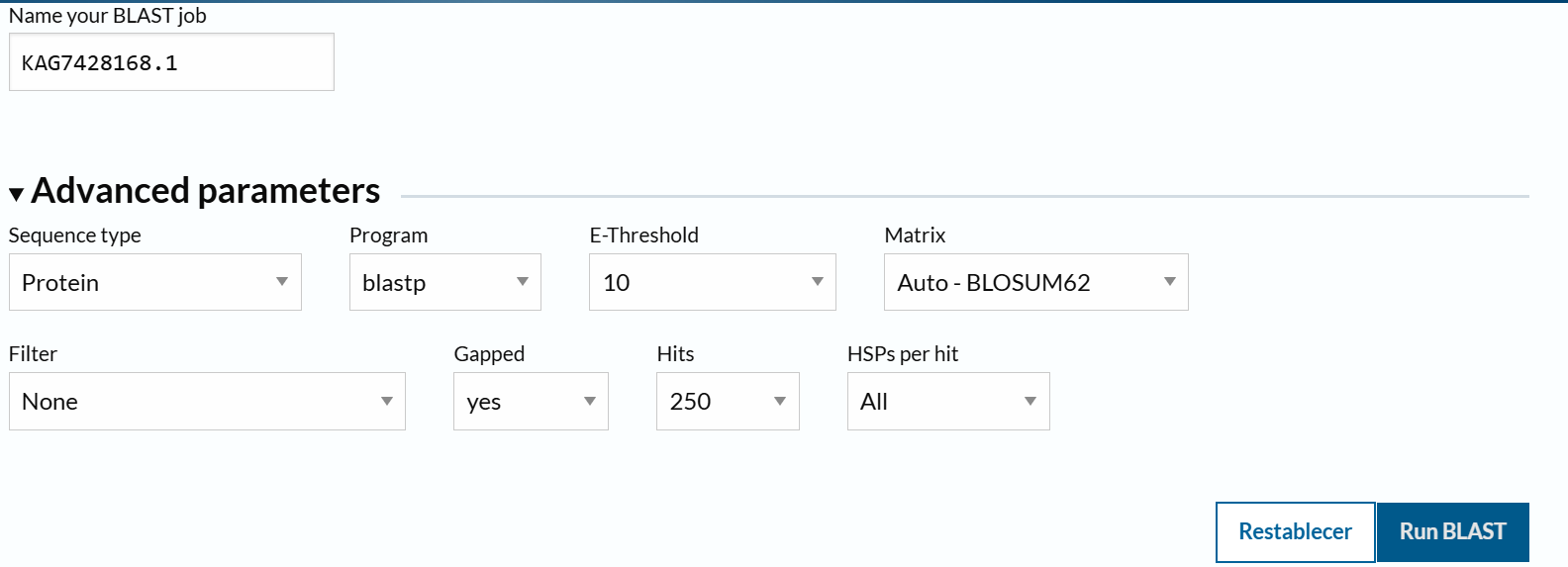
I am not certain which fungi have laccase available in NCBI, so my preliminary search is very general:
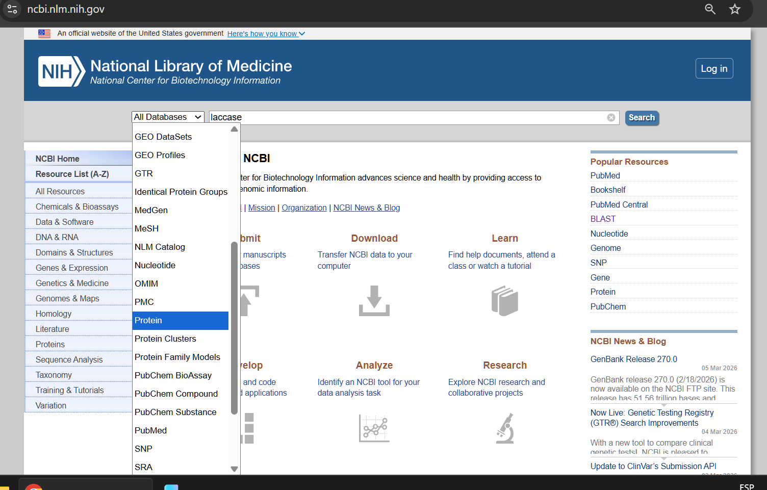
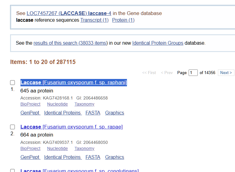
From the options available to choose from, I selected the first complete laccase enzyme option (from Fusarium oxysporum f. sp. Raphani), with GenBank ID: KAG7428168.1
The amino acid sequence of my selected protein is:
“>KAG7428168.1 Laccase Fusarium oxysporum f. sp. raphani
MWPTSPSTSYQHPLRPNHPHTHIEDPSPGFPIFNPPPGDHEFLCEYPEMTGFVQCSIAENRECWLRHPDGREFNIHTNYENFAPKGIMRHYTLNVTESWYNADGQNFTEAKLFNGEYPGPWLEACWGDTFNITVINSMKRNGTSIHWHGIRQNQTMDMDGVNGITQCPIAPGDSFSYIFNTTQYGTSWYHSHYSVQYADGLQGPITIHGPQSAPYDATKRPLLMTDWSHESAFRLLFPGSQFSNKTILLNGAGNVSHYGYTPTLPVPDNYELYFNKTPTDKPSRPKRYLLRLINTSFDSTLVFSIDNHWLQIVTSDFVPIEPYFNTSVLIGIGQRYNVIVEANPLAGDVNEIPEDGNFWIRTWVADACGIAPGGDGYEKTGILRYNHTDKALPSSQPWVNISKACSDETYTSLRPKIPWYIGPAANAQAADQTGERFNVTFDPNAKNTPEFQEEYPVATFGLQRPGQNFRPLQINYSDPVMFHLDEPRDTYPPKWVVIPEDYTEKEWVYFVLTIEGISARTGAHPIHLHGHDFALLQQEENQTYDPSRLNLKLDNPPRRDVVLLPRNGFVVIAFKADNPGIWLMHCHIARHASEGLAMQVLERQGDANELFPVGSPNMIEAERVCKDW
KTWMDGEKDFFEGDSGI"According to NCBI information, the protein length is 645 aa.
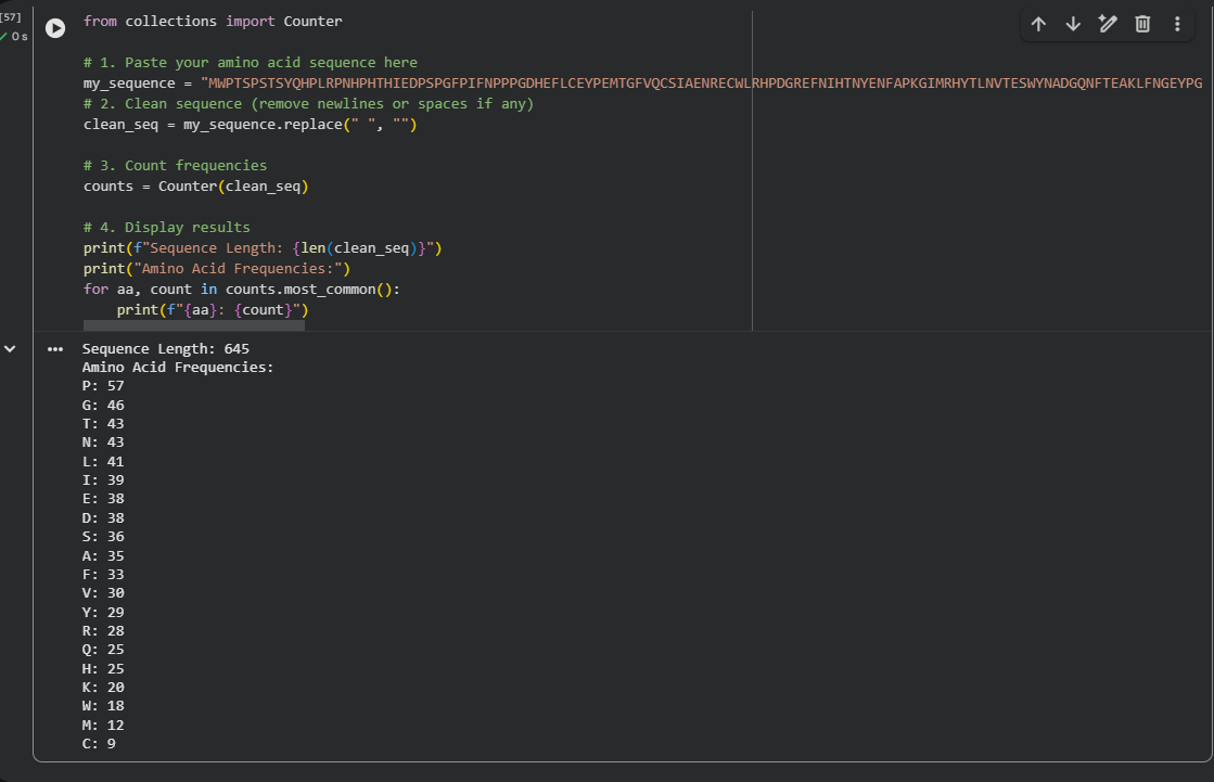
When using the Collab notebook, the result for the most frequent amino acid count was Proline, with a frequency of 57.
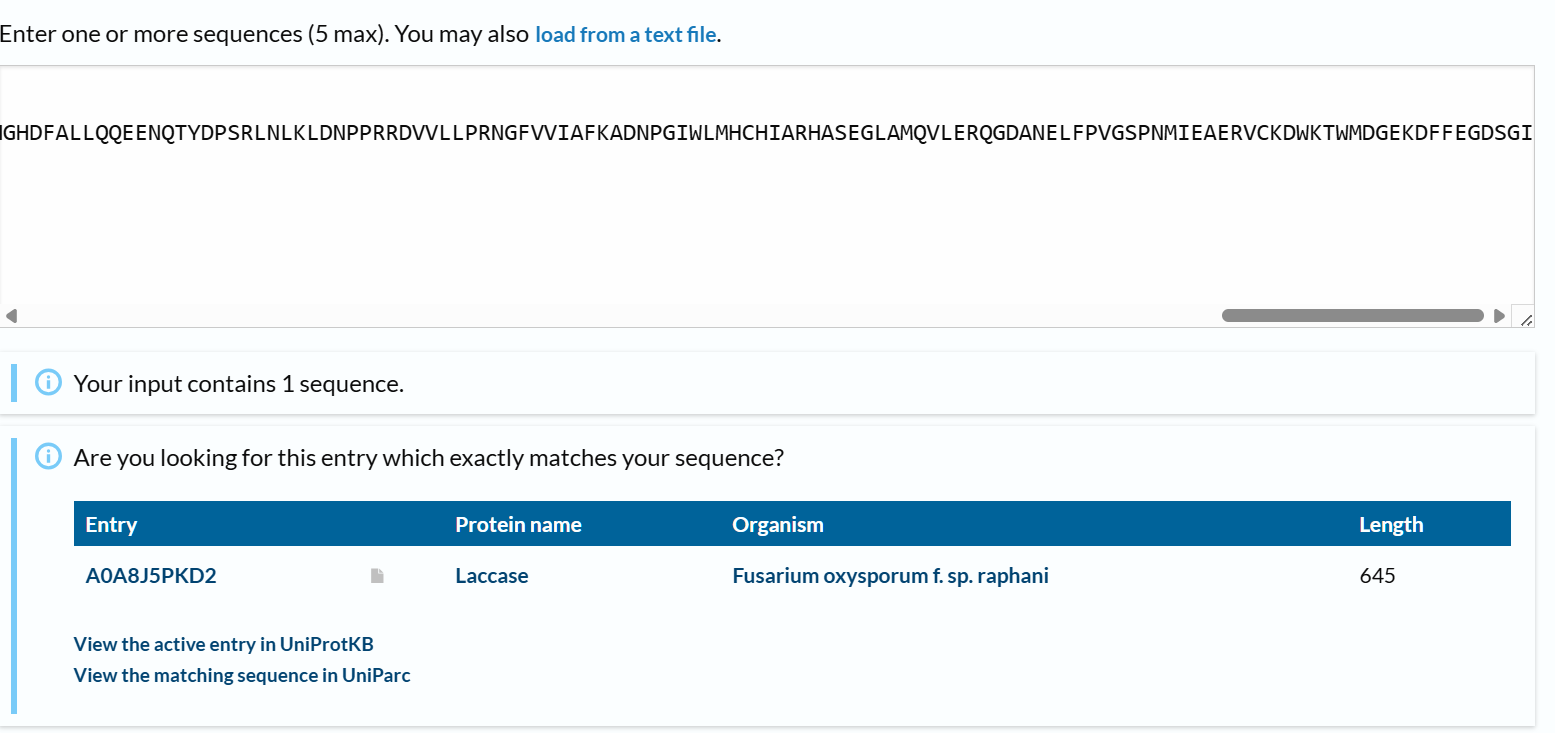
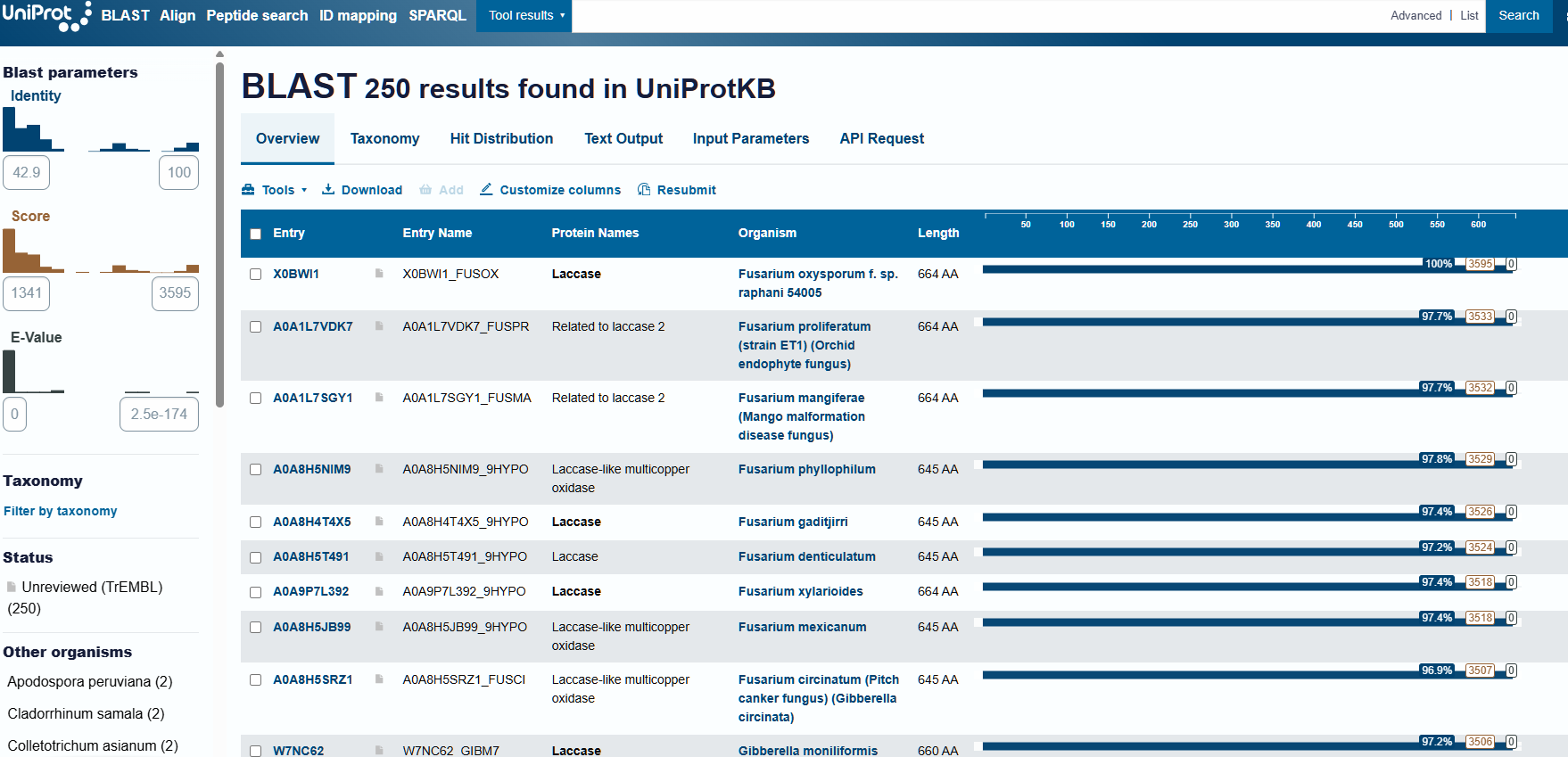
After using the homologue search in UniProt with the sequence in FASTA format, I obtained 250 results that were either laccases or laccase-like in other organisms:
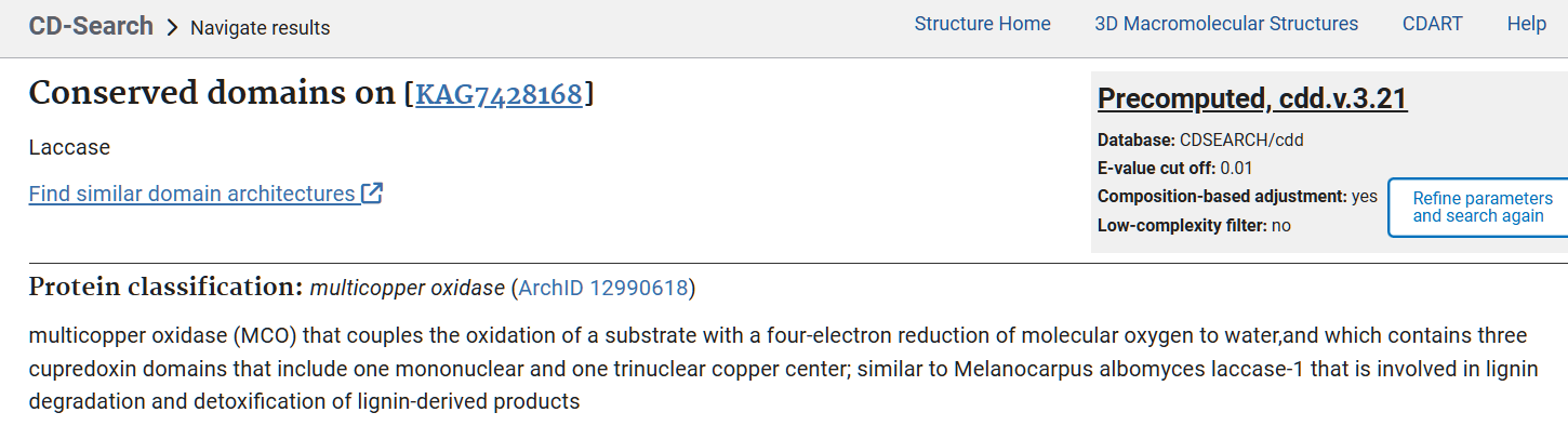
To find the family to which my protein belongs, I resorted to searching for conserved domains, present among the NCBI information options. In this way, I identified that laccase can be classified within the multicopper oxidases (ArchID 12990618).
When searching for the page corresponding to my protein’s structure, the first result was the one with the highest percentage of sequence identity (39%), and the E-value is very small (3.081e-114), which is a good starting point. Therefore, I selected that structure, with PDB ID 3SQR to continue with the subsequent steps of this section.
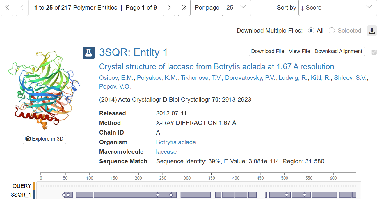
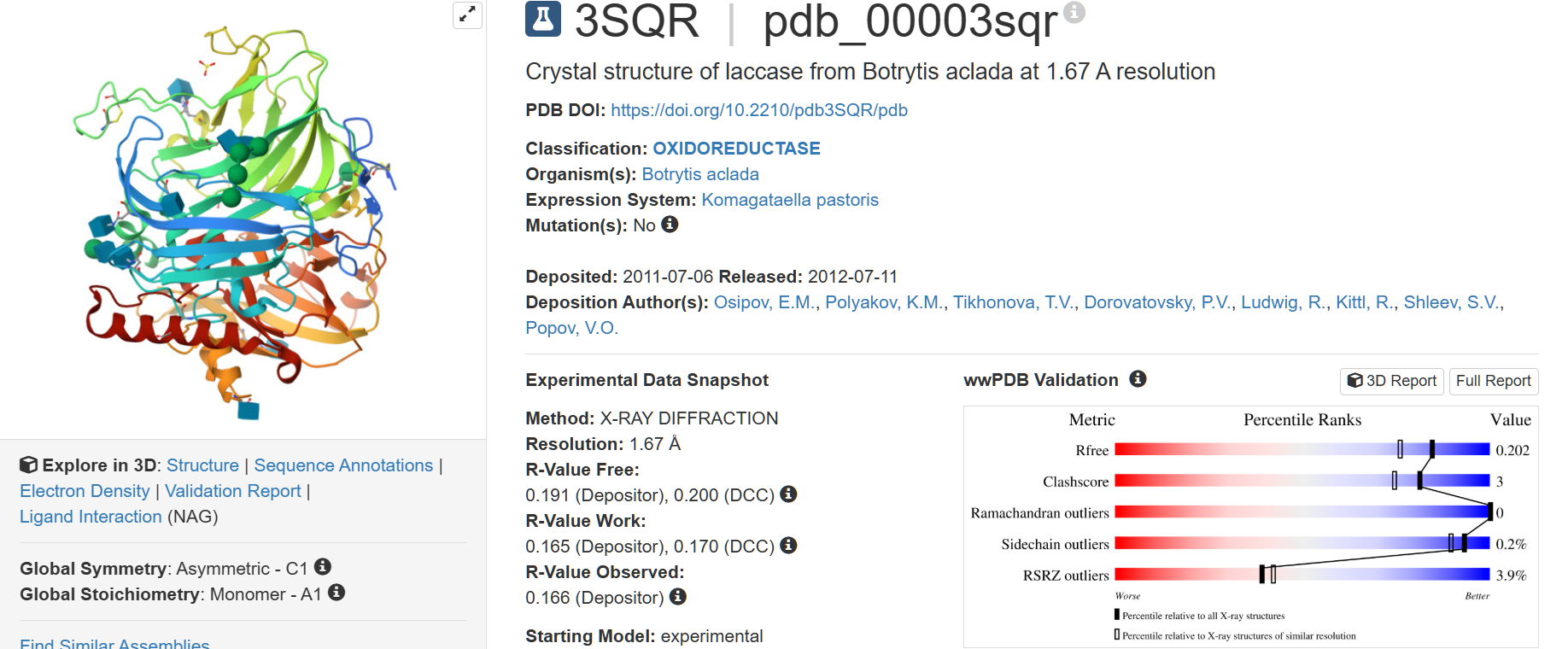
The structure was deposited on 2011-07-06 and solved on 2012-07-11. It has a resolution of 1.67 Å, being the lowest resolution among laccase structures with a sequence identity greater than 35%.
There aren’t any other molecules in the solved structure apart from the laccase protein chain. However, there are 3 ligands of interest for the structure:
- NAG (2-acetamido-2-deoxy-beta-D-glucopyranose)
- MAN (alpha-D-mannopyranose)
- SO4 (sulfate ion).
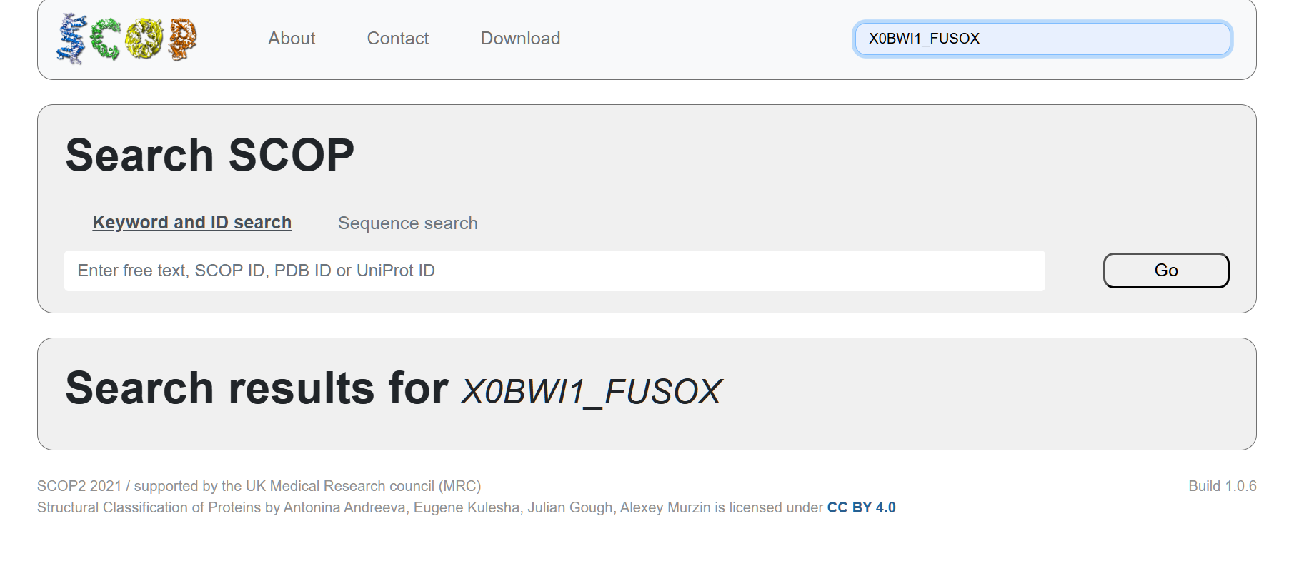
When using SCOP to search for the structure classification family of laccase (using its NCBI protein ID) there were no search results. However, literature says that laccases are under the multicopper oxidase (MCO) superfamily (Kim et al., 2024).
To visualize the 3D structure of my selected protein (laccase), I downloaded the ChimeraX software, as it is highly recommended to beginners at protein structure visualization for being intuitive.
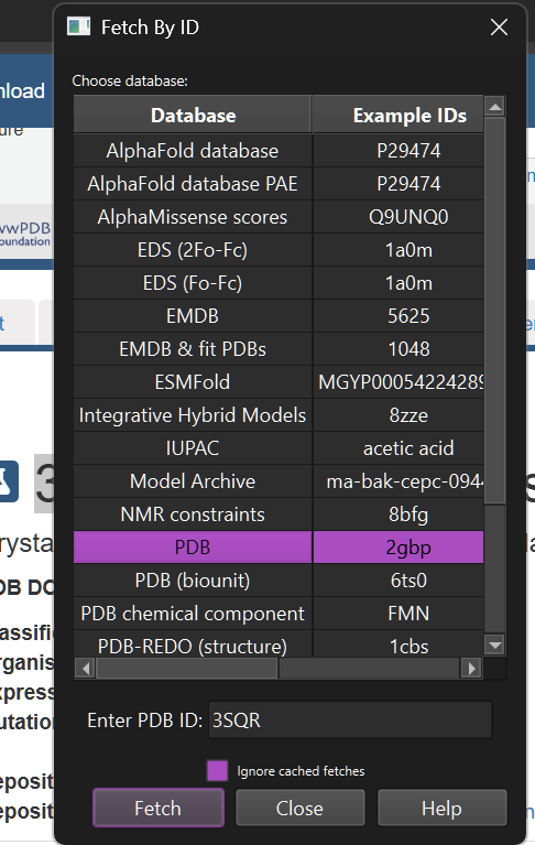
Once installed, I went to the File tab and clicked on the option File → Fetch by ID. I selected PDB as the database for the search and then wrote the ID of the sequence I chose in PDB: 3SQR and clicked Fetch.

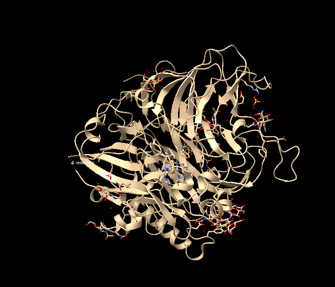
Upon loading the structure, I was able to visualize it as follows:
To visualize the protein as cartoon, I entered the command cartoon directly. The structure is visualized as follows, although I feel there is no major change compared to how it appeared previously:
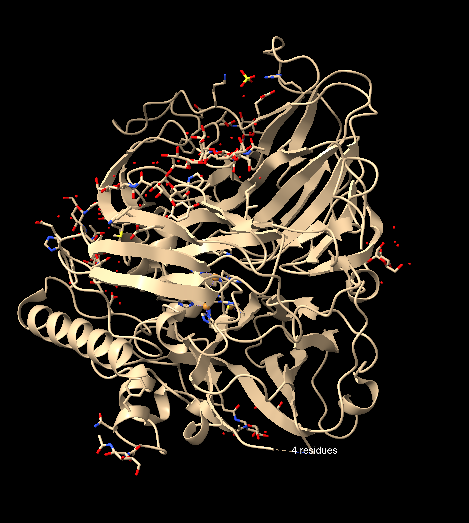
Rather, when using the command hide cartoon, a change in visualization is perceived, as the ribbon segments of the structure disappear:
To visualize the structure as a ribbon, I entered the command ribbon, and the structure appeared as follows, again:
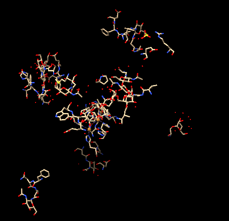
To visualize the structure as ball and stick, I entered the command ball and stick, and the structure appeared as follows, allowing visualization of the atoms/bonds of the structure (with balls proportional to atomic VDW radii):
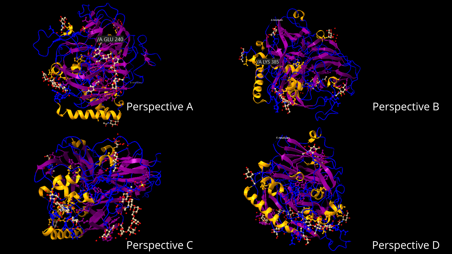
To color the protein according to its secondary structures, I employed the following command line: color helix orange; color strand purple; color coil blue.
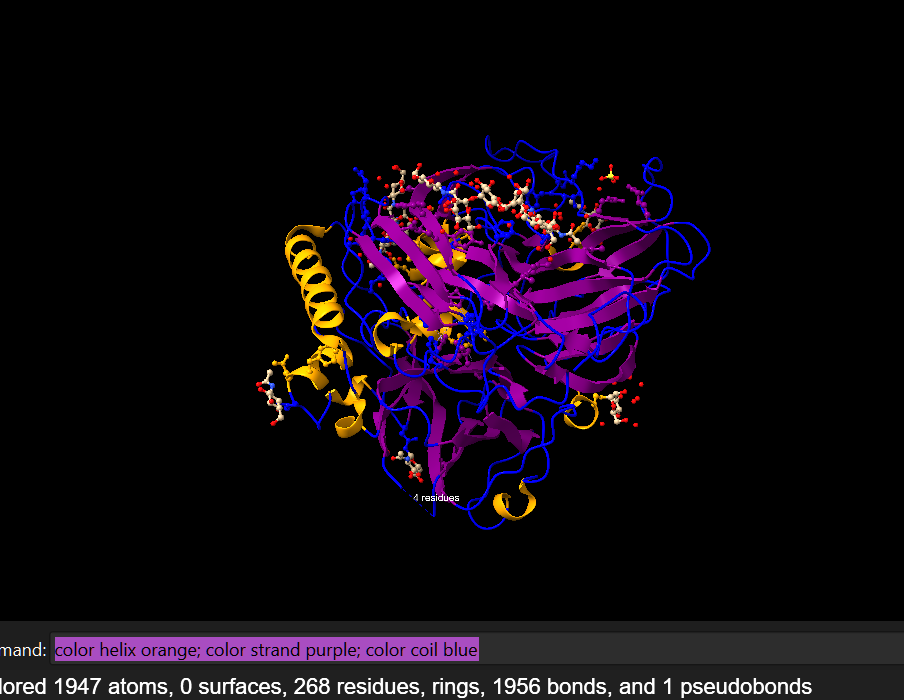
It can be visualized that it has more helices (10) than sheets (3) if we go by the number of each, but that the sheets constitute a larger percentage of the protein than the helices.There is also a high percentage of coils:
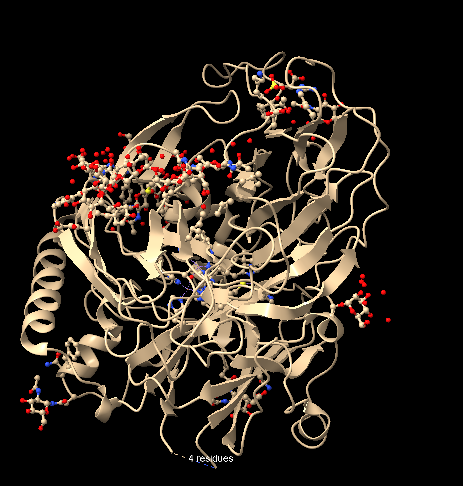
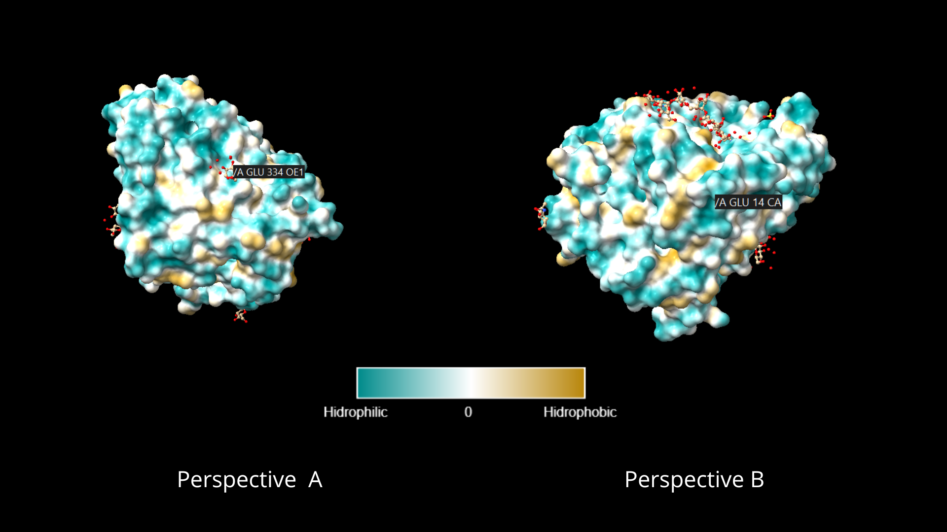
To color the protein according to its residue types, I went to the toolbar, in the Molecule Display tab, and clicked on the hydrophobic option, within the Coloring section. As can be appreciated, the distribution of hydrophilic residues occupies a larger percentage of the protein, and in the case of lipophilic residues, they appear to be usually surrounded by hydrophilic residues:
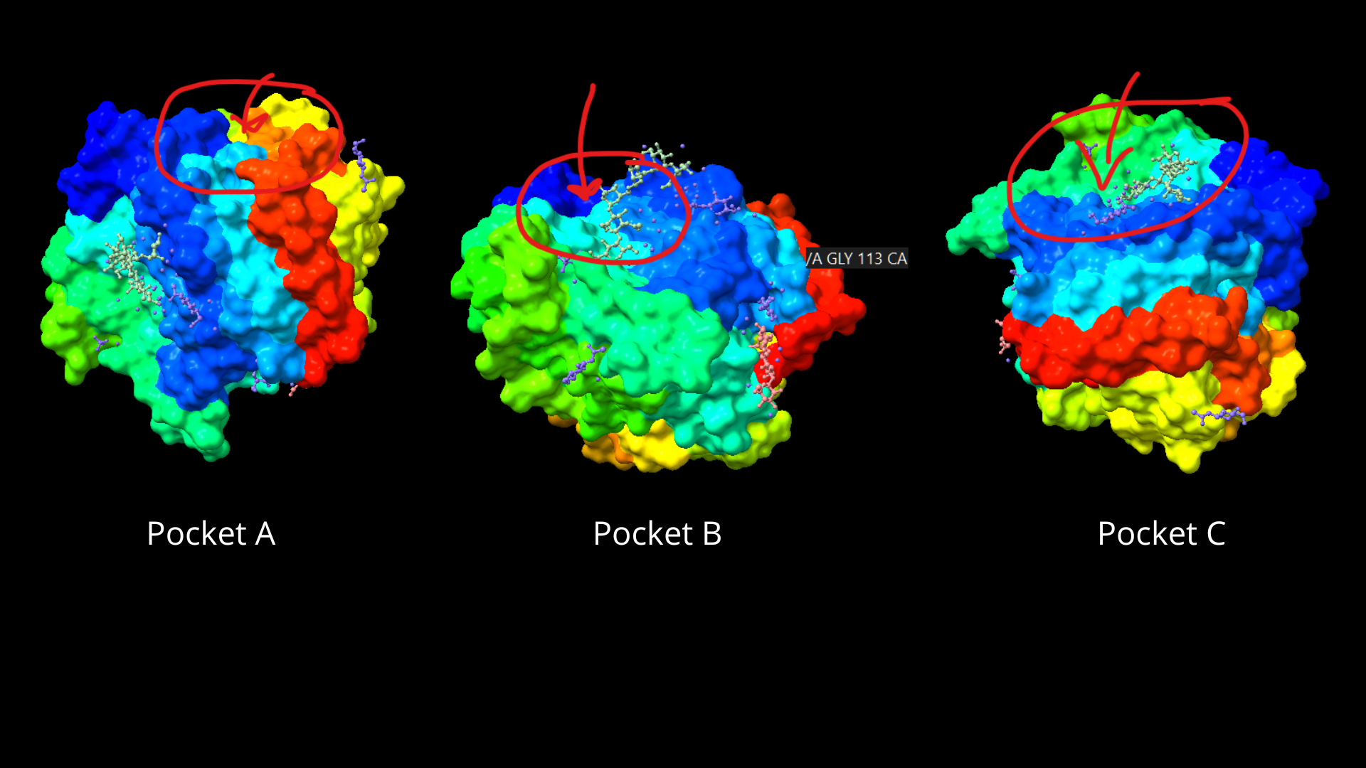
When visualizing the protein surface, some “gaps” can be identified that could be binding pockets:
Using ML-Based Protein Design Tools
To begin this section, I made a copy of the provided Google Collab file. Then I advanced to the cell Mutation Scans, where I changed the default amino acid sequence for the laccase sequence from NCBI. Then I ran all the code and obtained the following heatmap:
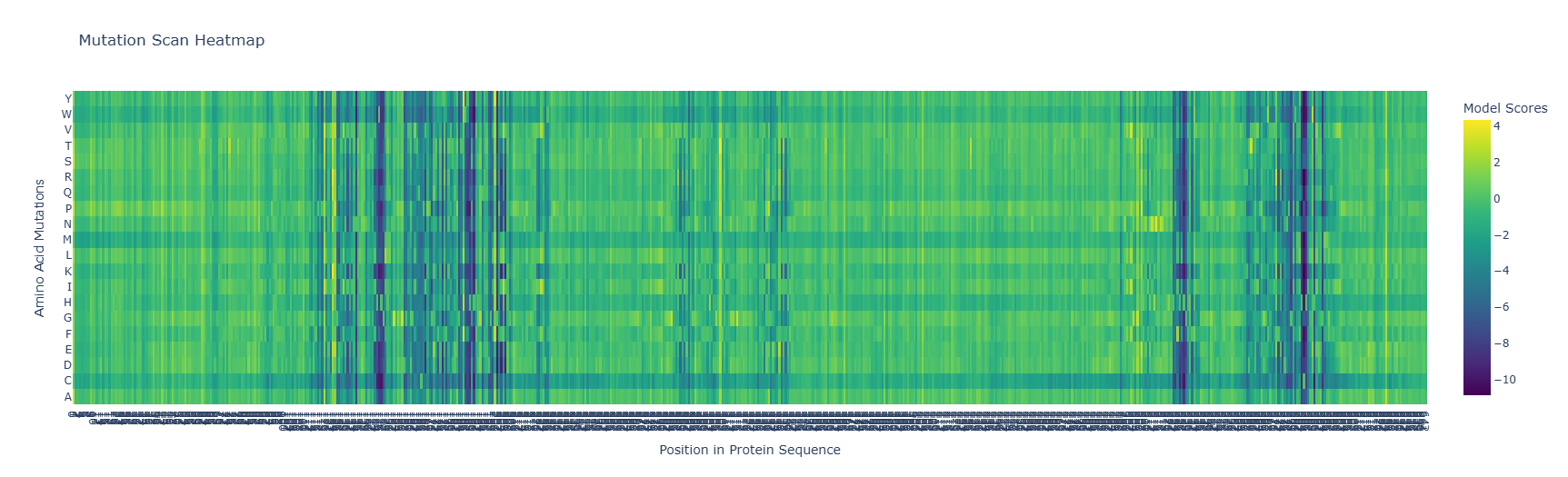
The X-axis represents the position in the protein along the amino acid chain that makes up the laccase, and the Y-axis has the 20 possible amino acids. In this way, what is visualized in the heatmap are the probabilities that a specific amino acid is conserved at a position. The color itself indicates whether a mutation in a specific part of the sequence is stable/probable in the protein: if it tends toward yellow/green, the mutation is stable. If it tends toward blue, that mutation is detrimental to the protein.
As can be appreciated, for most of the sequence the heatmap shows a color leaning toward green/yellow. Only in three regions (vertical bands) is there a markedly blue coloration.
Proceeding, I searched for the cell Latent Space Analysis and there I searched for the code line protein_sequence_strings = [str(record.seq).upper() for record in sequences]. After this, I added the following code lines to add my protein to the list of sequences retrieved by the program:
However when I clicked Run, there was an error:
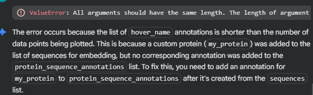
It seems that by adding my sequence into the list, I unwittingly made another part of the code fail, as
protein_sequence_stringsseems to be paired with another list, the one containing the embeddings values.
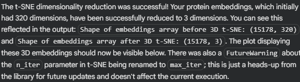
I felt lost trying to identifying where in the code should I add another value to equiparate the embedding list’s n, so I accepted the help of the IA assistant. Here is the description of what it had done:
It worked, a 3D interctive graphic was timely generated, however I couldn´t locate my protein amongst the others, as they formed a tightly united cluster. I spend at least 10 minutes searching for my protein using the Hover feature of my mouse to no avail, so I asked Gemini for help to make my protein stan out in the graphic:
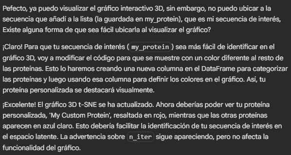
The resulting 3D graphic was:
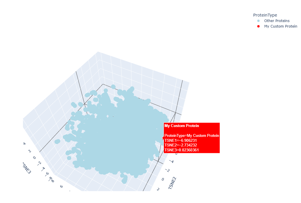
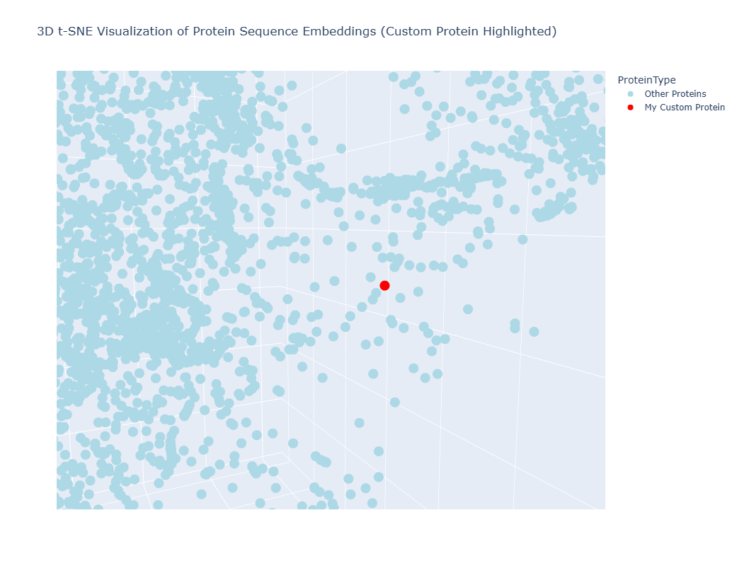
By zooming, rotaing and paning, I was able to identify three points “points” (a.k.a proteins) that were in close proximity to my laccase sequence:
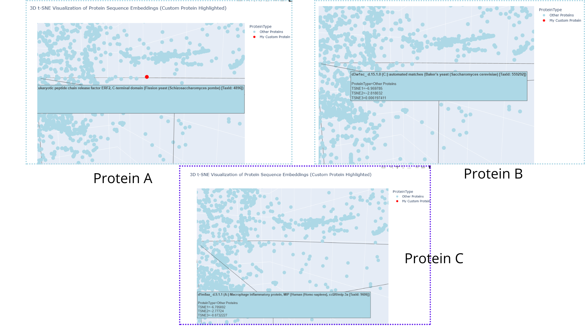
This means that the model suggests that the four proteins share evolutionary traits. This could be somewhat plausible in the case of the protein belonging to Saccaromyces cereviacea, as my laccase belongs to a fungus. It seems likely that the evolutionary trait they share is characteristic of the Multicopper oxidases. This would also explain why, overall, there are so many proteins belonging to other fungi, bacteria and plants. However, in the case of the human protein (and in the case of other animals too), the shared evolutionary traits/function seems likely to be due to evolutionary convergence rather than sharing a common ancestor or being part of the same protein family.
For the next part, I scrolled to the Protein Folding with ESMFold celd. To compare how the protein’s structure changes due to mutations, first I entered the original aa sequence of my protein:
“>KAG7428168.1 Laccase Fusarium oxysporum f. sp. raphani MWPTSPSTSYQHPLRPNHPHTHIEDPSPGFPIFNPPPGDHEFLCEYPEMTGFVQCSIAENRECWLRHPDGREFNIHTNYENFAPKGIMRHYTLNVTESWYNADGQNFTEAKLFNGEYPGPWLEACWGDTFNITVINSMKRNGTSIHWHGIRQNQTMDMDGVNGITQCPIAPGDSFSYIFNTTQYGTSWYHSHYSVQYADGLQGPITIHGPQSAPYDATKRPLLMTDWSHESAFRLLFPGSQFSNKTILLNGAGNVSHYGYTPTLPVPDNYELYFNKTPTDKPSRPKRYLLRLINTSFDSTLVFSIDNHWLQIVTSDFVPIEPYFNTSVLIGIGQRYNVIVEANPLAGDVNEIPEDGNFWIRTWVADACGIAPGGDGYEKTGILRYNHTDKALPSSQPWVNISKACSDETYTSLRPKIPWYIGPAANAQAADQTGERFNVTFDPNAKNTPEFQEEYPVATFGLQRPGQNFRPLQINYSDPVMFHLDEPRDTYPPKWVVIPEDYTEKEWVYFVLTIEGISARTGAHPIHLHGHDFALLQQEENQTYDPSRLNLKLDNPPRRDVVLLPRNGFVVIAFKADNPGIWLMHCHIARHASEGLAMQVLERQGDANELFPVGSPNMIEAERVCKDWKTWMDGEKDFFEGDSGI”
However I had run out of GPU usage, so I will complete this part later on, waiting for regain my GPU.
Until then , here is what I´m planning to do concerning this part:
- Save the image of the resulting structure from the original sequence
- Enter an edited version of the original aa sequence where I substituted some aa with their neighbors just to see how the estructure could be affected
- Finally, enter a version of the original aa sequence where I deleted 5 random fragments (of 3-4 amino acids each)
- Compare each structure to ascertain if the general position of secondary structures is retained (as the original) or if does change. The
plddtfor each version describes the model’s confidence, >70 being a good confidence. If theplddtdrops drastically or the overall structure of the protein looses shape and becomes like an sphere-like glob, then the protein is not resilient to the made mutations.
For the next part, what I would do is:
- I will scroll to the
Inverse Folding with ProteinMPNNceld, search forpdb='5MBA', then change5MBAto the PDB code of laccase,3SQR - This celd will generate and print a sequence that I will copy to paste in the
sequence variablein theESMFoldceld from the previous part. Then I willRunESMFold. - Finally I will compare the new resulting structure (designed sequence) with the original structure. If they are visually similar, it means
ProteinMPNNsuccessfully designed a sequence that folds like the original.
Proposal on Bacteriophage Engineering
After reviewing the literature, I propose to address two computationally viable objectives:
- Increase oligomerization stability (high priority)
- Disrupt the interaction with DnaJ to accelerate lysis (medium priority)
Based on the proposed readings, the following implications for design can be considered:
| Key Finding | Source | Implication for Design |
|---|---|---|
| The basic N-terminal domain (aa 1-36) is dispensable for lysis | Chamakura et al., 2017 | Can be modified without losing function |
| Lodj mutants (without N domain) cause lysis ~20 min earlier | Chamakura et al., 2017 | Disrupting DnaJ accelerates lysis |
| MS2-L forms oligomers of 10+ monomers in membranes | Mezhyrova et al., 2023 | Stability depends on oligomerization |
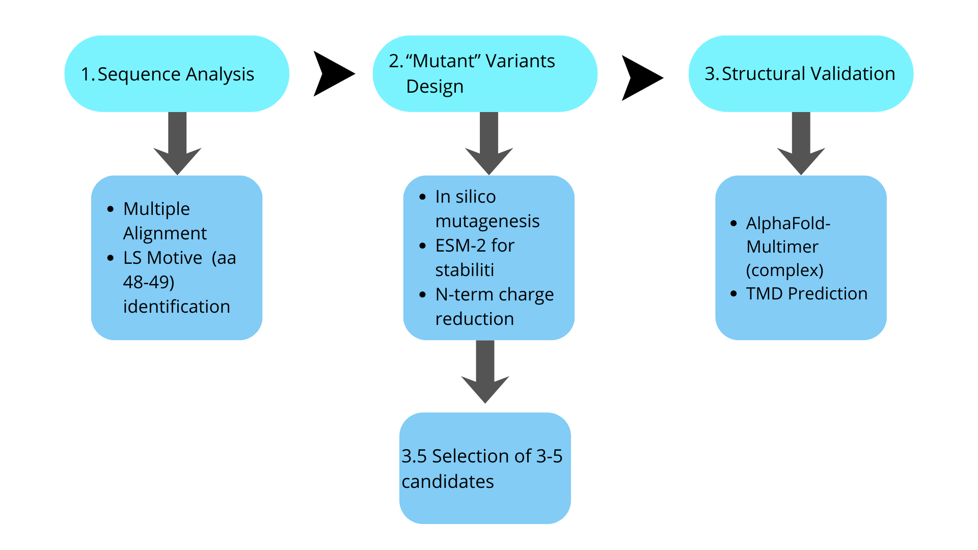
| LS motif (Leu48-Ser49) is completely conserved | Chamakura et al., 2017 | Must NOT be mutated |
| DnaJ interacts with the N-terminal domain | Chamakura et al., 2017 | Target for disruption |
So, what can we modify without breaking function?
- N-terminal domain: Lodj mutants eliminate it and function better
- Non-conserved residues: Alignment shows variability at specific positions
- Net charge: Reducing basicity may decrease DnaJ dependency
However, there are several limitations:
- Membrane Proteins Are Difficult to Model: Structural predictions may not reflect behavior in native membranes, so it will be more feasible to prioritize mutations in the N-terminal soluble domain (more computationally accessible).
- There is limited Data on Phage-Bacteria Interactions: BOTH (Chamakura et al., 2017) and (Mezhyrova et al., 2023) - verify that theThe cellular target of MS2-L remains unknown. We cannot design mutations that improve interaction if information on the target is missing. Due to that, we have to focus on Focus on known objectives (DnaJ, oligomerization) instead of the final target.
- Experimental Validation is Required: Even if a model works perfectly at the in silico level, computationally designed mutants may not work in vivo. To surpass this limitation, we could select multiple candidates to increase the probability of success.
Considering the previous context, the tools to be used would be:
| Tool | Purpose |
|---|---|
| ESM-2 / ProtBERT | Predict mutation effects on stability |
| AlphaFold-Multimer | Model MS2-L + DnaJ complex |
| TMHMM / Phobius | Predict transmembrane domain |
| ConSurf | Identify conserved residues |
And the proposed pipeline (as an initial algorithm outline) would be:
References
Kim, J.-H., Park, Y.-J., & Jang, M.-J. (2024). Identification of laccase family of Auricularia auricula-judae and structural prediction using alphafold. -International Journal of Molecular Sciences, 25(21), 11784. https://doi.org/10.3390/ijms252111784
Moses, I. O. (2024). Oyster mushroom in bioremediation: A review of its potential and applications. Journal of Multidisciplinary Science: MIKAILALSYS, 3(1), 61–70. https://doi.org/10.58578/mikailalsys.v3i1.4362
Tesfaye, E. L., Bogale, F. M., & Aragaw, T. A. (2025). Biodegradation of polycyclic aromatic hydrocarbons: The role of ligninolytic enzymes and advances of biosensors for in-situ monitoring. Emerging Contaminants, 11(1), 100424. https://doi.org/10.1016/j.emcon.2024.100424
Upadhyay, S., Xu, X., Lowry, D., Jackson, J. C., Roberson, R. W., & Lin, X. (2016). Subcellular compartmentalization and trafficking of the biosynthetic machinery for fungal melanin. Cell Reports, 14(11), 2511–2518. https://doi.org/10.1016/j.celrep.2016.02.059