Week 10 HW: Imaging And Measurement

My project aims to express the carbon monoxide dehydrogenase (CODH) pathway from Oligotropha carboxidovorans in Nicotiana tabacum (tobacco) using a two-plasmid system. I need to measure whether the system works at every level — from DNA integration to enzyme function to plant health. Below i included what I will measure, how I will measure it, and the technologies I will use:
1. Confirming DNA Integration and Sequence
What I measure: Whether the seven CODH genes are present in the tobacco genome and whether their sequences are correct.
How I measure it:
- Genomic PCR: Extract DNA from leaves, design primers specific to each of my seven codon-optimized genes, run PCR, and look for bands on an agarose gel.
- Border-specific PCR: Use one primer in the T-DNA border (LB or RB) and one primer in my gene to confirm the entire T-DNA integrated.
- Sanger sequencing: Send PCR products to a sequencing facility, align the returned sequences against my Benchling design using SnapGene.
image ref

Technologies: PCR thermocycler, agarose gel electrophoresis, UV transilluminator, Sanger sequencing service, sequence alignment software.
2. Confirming mRNA Transcription
What I measure: Whether the seven genes are being transcribed into mRNA, and whether the three structural subunits (CoxL, CoxM, CoxS) are expressed at balanced levels.
How I measure it:
- Extract total RNA from leaves using an RNA extraction kit.
- Treat with DNase to remove genomic DNA.
- Convert mRNA to cDNA using reverse transcriptase.
- Run qPCR with gene-specific primers and SYBR Green.
- Include reference genes for normalization.
- Compare Ct values across the three structural subunits.
Technologies: RNA extraction kit, DNase, reverse transcriptase, qPCR machine, SYBR Green.
image ref

3. Confirming Protein Presence and Assembly
What I measure: Whether CoxL, CoxM, and CoxS are present, whether the chloroplast transit peptide was cleaved, and whether the three subunits assemble into the complex.
How I measure it:
- Isolate intact chloroplasts using Percoll gradient centrifugation.
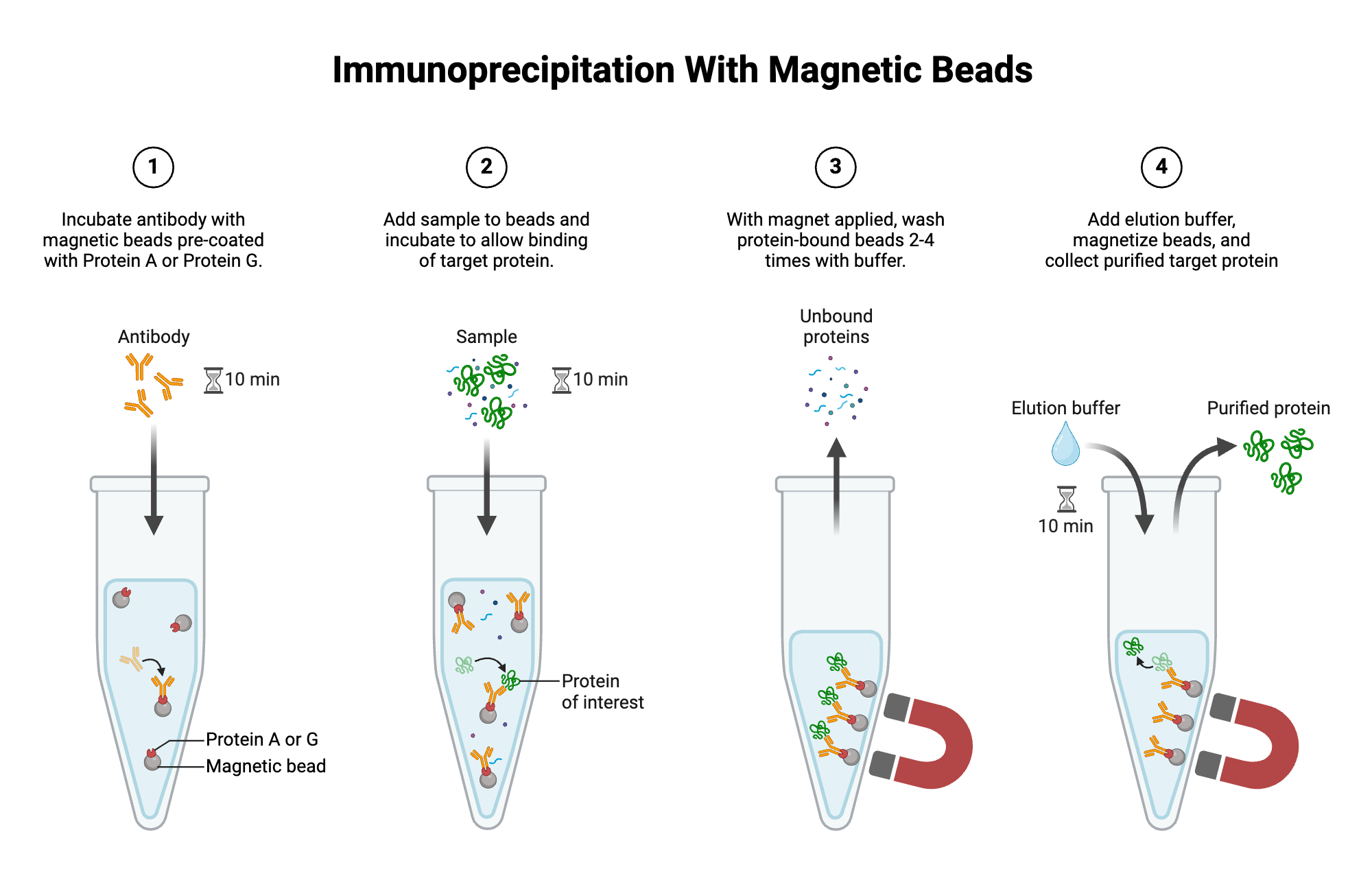
- Lyse chloroplasts gently and perform Co-IP using anti-FLAG magnetic beads (FLAG is on CoxS).
- Elute with FLAG peptide.
- Split eluate: run on Tricine-SDS-PAGE (silver stain) to see individual subunits at 88 kDa (CoxL), 32 kDa (CoxM), and 18 kDa (CoxS) (Denatured conditions).
- Run on Blue Native PAGE (Coomassie stain) to see the assembled complex at ~280 kDa (Undenatured conditions).
- For maturation proteins: run anti-FLAG Western (detects CoxD) on total chloroplast extract.
Technologies: Ultracentrifuge, anti-FLAG magnetic beads, PAGE equipment, silver stain, Coomassie stain, Western blot transfer system, chemiluminescence imager.


4. Confirming Chloroplast Targeting
What I measure: Whether the used chloroplast transit peptides direct proteins to the chloroplast.
How I measure it:
- Build a separate reporter construct: promoter + CTP + GFP + terminator.
- Transform into tobacco, select on hygromycin.
- Take fresh leaf samples, mount on slides with water.
- Observe under confocal microscope: GFP channel (green) and chlorophyll autofluorescence (red).
- Calculate Pearson’s correlation coefficient using ImageJ (target >0.7).
Technologies: Confocal laser scanning microscope, ImageJ software.
image ref

5. Confirming CO Oxidation Activity
What I measure: Whether the assembled CODH enzyme can oxidize CO to CO₂.
How I measure it:
- Gas phase (whole plant): Place transformed plant in sealed transparent chamber, inject CO gas, record CO concentration in separate timelines using electrochemical CO sensor.
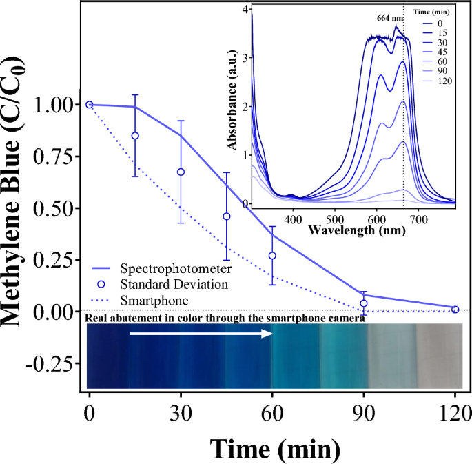
- Methylene blue (purified enzyme): Purify CODH complex via anti-FLAG Co-IP, add to reaction with methylene blue and CO in anaerobic cuvette, measure absorbance at 600 nm at different timelines. Calculate specific activity (μmol CO/min/mg protein).
Technologies: Sealed gas chamber, electrochemical CO sensor, spectrophotometer, anaerobic cuvettes.
image ref
6. Confirming Cofactor Incorporation
What I measure: Whether the CODH complex contains molybdenum, copper, and iron-sulfur clusters.
How I measure it:
- ICP-MS: Send purified CODH complex to core facility. Measure Mo, Cu, and Fe content. Calculate metal-to-protein stoichiometry.
- UV-Vis spectroscopy: Measure absorbance spectrum of purified complex from 300-700 nm. Look for peak at 420 nm (Fe-S clusters).
Technologies: ICP-MS instrument, UV-Vis spectrophotometer.
7. Confirming Electron Transfer Compatibility
What I measure: Whether electrons from CODH go to the photosynthetic electron transport chain or leak to oxygen.
How I measure it:
- Compare CO oxidation rate in light vs. dark using the gas chamber setup.
- Calculate light:dark ratio. Ratio >2 indicates electrons go to photosynthetic chain (requires light). Ratio ~1 indicates electrons go directly to oxygen (oxidative stress risk).
Technologies: Sealed gas chamber, electrochemical CO sensor, light source, dark cover.
8. Monitoring Plant Health
What I measure: Whether expressing CODH causes stress or benefits photosynthesis.
How I measure it:
- Chlorophyll fluorescence (Fv/Fm): Dark-adapt leaf for 20 minutes, measure with PAM fluorometer. Healthy plant = 0.80-0.83.
- CO₂ assimilation: Use infrared gas analyzer (IRGA) to measure net CO₂ uptake by leaf. Compare transformed vs. wild-type.
- Biomass: Dry plants at 70°C for 48 hours, weigh shoot and root. Compare transformed vs. wild-type.
- ROS detection: Stain leaf discs with NBT (detects superoxide, turns blue) and DAB (detects H₂O₂, turns brown). Photograph and quantify staining.
Technologies: PAM fluorometer, LI-COR IRGA, analytical balance, NBT/DAB staining, light microscope, ImageJ.
image ref

image ref
 Histochemical detection of H2O2 by DAB staining (a), superoxide radical by NBT staining (b)
9. Monitoring Silencing Over Time
What I measure: Whether expression remains stable across generations (T0 → T1 → T2).
How I measure it:
- Grow T0 plants (primary transformants), measure mRNA by RT-qPCR.
- Self-pollinate T0 to obtain T1 seeds.
- Grow T1 plants, repeat RT-qPCR.
- Grow T2 plants, repeat RT-qPCR.
- Calculate silencing index = Expression(T1)/Expression(T0). Index >0.8 = stable.
Technologies: RT-qPCR, plant growth facilities.
Homework: Waters Part I — Molecular Weight
Assignees for this section
- MIT/Harvard students Required
- Committed Listeners Required
We will analyze an eGFP standard on a Waters Xevo G3 QTof MS system to determine the molecular weight of intact eGFP and observe its charge state distribution in the native and denatured (unfolded) states. The conditions for LC-MS analysis of intact protein cause it to unfold and be detected in its denatured form (due to the solvents and pH used for analysis).
- Based on the predicted amino acid sequence of eGFP (see below) and any known modifications, what is the calculated molecular weight? You can use an online calculator like the one at https://web.expasy.org/compute_pi/ eGFP Sequence: MVSKGEELFTG VVPILVELDG DVNGHKFSVS GEGEGDATYG KLTLKFICTT GKLPVPWPTL VTTLTYGVQC FSRYPDHMKQ HDFFKSAMPE GYVQERTIFF KDDGNYKTRA EVKFEGDTLV NRIELKGIDF KEDGNILGHK LEYNYNSHNV YIMADKQKNG IKVNFKIRHN IEDGSVQLAD HYQQNTPIGD GPVLLPDNHY LSTQSALSKD PNEKRDHMVL LEFVTAAGIT LGMDELYKLE HHHHHH Note: This contains a His-purification tag (HHHHHH) and a linker (the LE before it).
- Calculate the molecular weight of the eGFP using the adjacent charge state approach described in the recitation. Select two charge states from the intact LC-MS data (Figure 1) and:
- Determine z for each adjacent pair of peaks (n,n+1) using: n = (m/z(n+1)−1)/(m/z(n)−m/z(n+1))
- Determine the MW of the protein using the relationship between m/zn, MW and z.
- Calculate the accuracy of the measurement using the deconvoluted MW from 2.2 and the predicted weight of the protein from 2.1 using: Accuracy = (|Calculated MW – Theoretical MW|) / (Theoretical MW) x 1,000,000
- Can you observe the charge state for the zoomed-in peak in the mass spectrum for the intact eGFP? If yes, what is it? If no, why not?
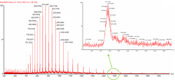 Figure 1. Mass Spectrum of intact eGFP protein from the Waters Xevo G3 LC-MS (a mass spectrometer with 30,000 resolution) with individual charge state peaks labeled with m/z values.
- Theoretical Molecular Weight Calculation
The theoretical molecular weight of eGFP was calculated using the online tool ExPASy Compute pI/Mw tool (Swiss Institute of Bioinformatics). The full amino acid sequence of eGFP, including the C-terminal His-tag (HHHHHH) and linker (LE), was entered into the calculator.
 The computed molecular weight obtained from this tool was: 28006.60 Da
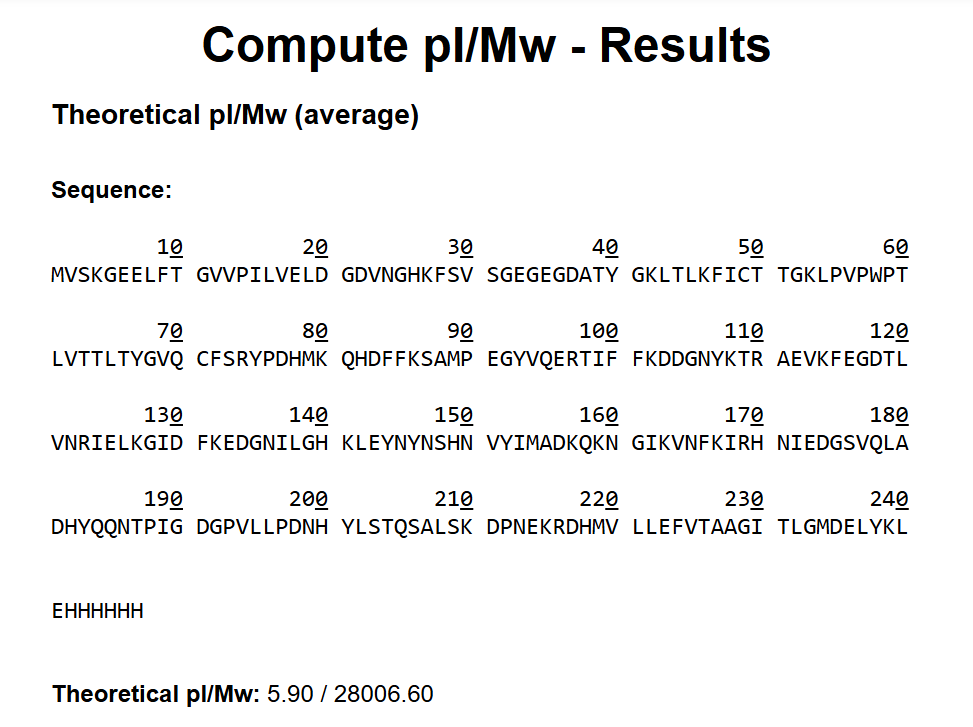 This value was used as the reference theoretical mass for comparison with the experimentally determined molecular weight obtained from LC-MS analysis.
Calculating the Experimental Molecular Weight (MW)
2.1. Identification of Adjacent Charge States
Step 1: Identifing Two Adjacent Peaks from Figure 01
let’s use the following values from this figure:
m/z(n) = 903.7148
m/z(n+1) = 875.4421
Step 2: Solve for the Charge State (n)
The relationship between the two peaks is:
n = (m/z(n+1)−1)/(m/z(n)−m/z(n+1))
Let’s plug in our example numbers:
n = 875.4421 – 1 / (903.7148 – 875.4421)
n = 874.4421/ (28.2727)
n = 30.93
Since the charge state must be a whole integer, we round this to the nearest whole number. Therefore, n = 31. This means the peak at m/z 903.7148 is the +31 charge state. From this value, we can extract the charge state for the second adjacent peak: n+1 = 32, which means the peak at m/z 875.4421 is the +32 charge state.
2.2. Calculating (MW)
Now that we know n, we can calculate M using the following formula, which accounts for the mass of the protons that are adding the charge:
m/z = MW of protein + mass of all added protons / total number of charges (n)
MW of protein = (m/z x total number of charges (n)) – (mass of all added protons)
Note: mass of all added protons is: the total number of charges (n) x the mass of a proton (approximately 1.0078 Da) (H)
Using the charge state of the first peak:
MW = (m/z(n) x zn) – (zn x H)
MW = (875.4421 x 32) - (32 x 1.0078)
MW = 28014.1472 – 32.2496
MW = 27981.8976 Da
Using the second peak, I found: MW = 27983.917 Da, so the average experimental molecular weight of this protein is ≈ 27982.9073 Da By comparing the experimental result, we just calculated to the theoretical weight from Step 1, the resulted experimental molecular weight is approximate to the theoretical value calculated 28006.60 Da.
2.3. Calculating the Measurement Accuracy
The formula for accuracy is:
Accuracy = (|Calculated MW – Theoretical MW|) / (Theoretical MW) x 1,000,000
Accuracy = (|27982.9073 – 28006.60 |) / (28006.60) x 1,000,000
Accuracy = (9.56) / (28006.60) x 1,000,000
Accuracy = 845.96 ppm > 50 ppm
The measured accuracy (~846 ppm) is significantly higher than the acceptable threshold of 50 ppm.
This deviation is most likely due to instrumental factors, such as imperfect calibration of the mass spectrometer, which can lead to slight inaccuracies in measured m/z values. Since the theoretical mass was calculated directly from the provided amino acid sequence, it is unlikely that the discrepancy arises from errors in the protein sequence or its expression.
- Charge State Determination (Zoomed Peak)
No, we cannot. The inability to determine the charge state from the zoomed-in peak is mainly due to the relationship between isotope spacing and instrument resolution. Proteins are made of atoms that exist in different isotopic forms, such as 12C and 13C, which create small differences in mass. In their neutral state, these isotopes are separated by about 1 Da. However, in mass spectrometry, we measure the mass-to-charge ratio (m/z), so the space between isotopic peaks becomes (1/z), where (z) is the charge. This means that as the charge increases, the spacing between peaks becomes smaller.
For large proteins like eGFP (approximately 28 kDa), the charge state is relatively high. As a result, the spacing between isotopic peaks becomes extremely small. For example, if the charge is around (z ≈ 19), the spacing between peaks is only about 0.05 (m/z). These very small differences are difficult for the instrument to detect.
The limitation comes from the resolution of the mass spectrometer. Resolution refers to the ability of the instrument to distinguish between two very close peaks. In this case, the required spacing (around 0.05 (m/z)) is smaller than what the instrument can clearly resolve. Instead of observing distinct isotopic peaks, the signals merge together and appear as a single broad and jagged peak.
Because the individual isotope peaks are not visible, it is not possible to measure their spacing and determine the charge state directly. Therefore, an alternative approach, such as the adjacent charge state method, must be used to calculate the charge and molecular weight.
Homework: Waters Part II — Secondary/Tertiary structure
Assignees for this section
- MIT/Harvard students Required
- Committed Listeners Required
We will analyze eGFP in its native, folded state and compare it to its denatured, unfolded state on a quadrupole time-of-flight MS. We will be doing MS-only analysis (no liquid chromatography, also known as “direct infusion” experiments) on the Waters Xevo G3-QToF MS.
- Based on learnings in the lab, please explain the difference between native and denatured protein conformations. For example, what happens when a protein unfolds? How is that determined with a mass spectrometer? What changes do you see in the mass spectrum between the native and denatured protein analyses (Figure 2)?
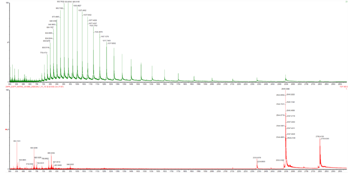 Figure 2. Comparison of the mass spectra between denatured (top) and native (bottom) eGFP standard on the Waters Xevo G3 QTof MS.
 - Zooming into the native mass spectrum of eGFP from the Waters Xevo G3 QTof MS (see Figure 3), can you discern the charge state of the peak at ~2800 ? What is the charge state? How can you tell?
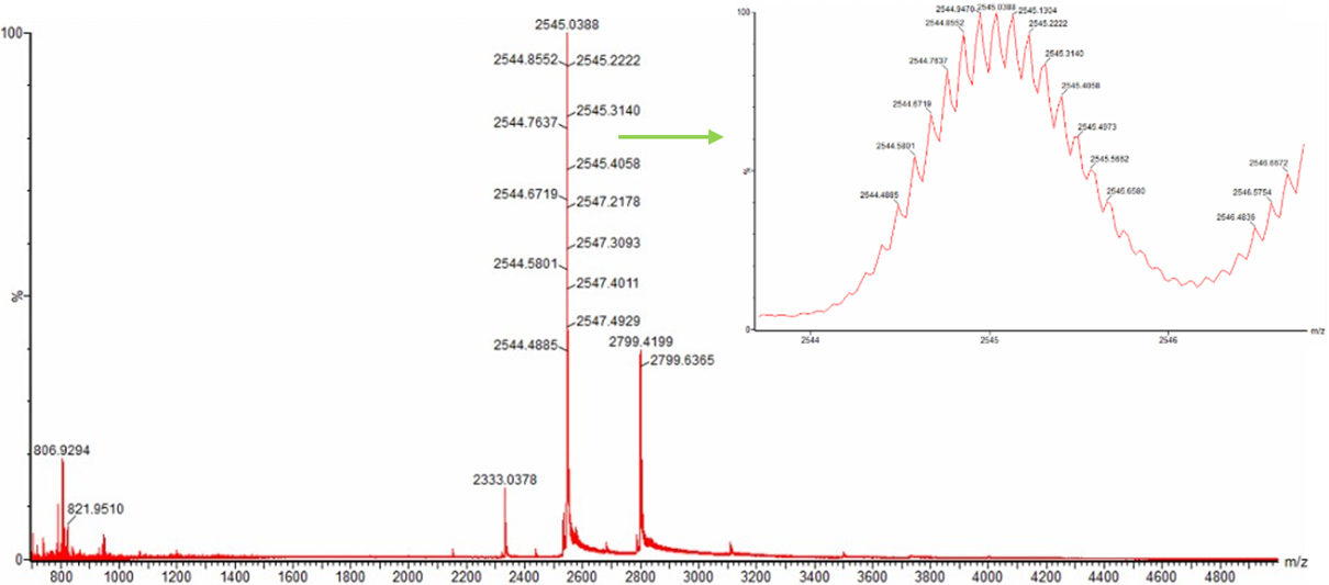 Figure 3. Native eGFP mass spectrum from the Waters Xevo G3 Q-Tof MS. The inset is a zoomed-in view of the charge state at ~2800 m/z on a mass spectrometer with 30,000 resolution.
- the difference between native and denatured protein conformations
What happens when a protein unfolds?
In its native state, a protein such as eGFP is folded into a compact three-dimensional structure (often described as a beta-barrel). In this conformation, many basic amino acid residues (such as lysine and arginine) are buried inside the protein and are not easily accessible. When the protein becomes denatured, typically due to acidic or organic solvents, it loses this structure and unfolds into a more extended chain. This unfolding exposes a larger surface area and reveals previously hidden basic sites.
How is this determined with a Mass Spectrometer?
Mass spectrometry detects the charge-to-mass ratio (m/z). Because an unfolded protein has more surface area and more exposed basic sites, it can pick up a much higher number of protons (H+) during Electrospray Ionization (ESI). So, in simple way:
- Native (folded) protein: Compacted structure → Fewer exposed basic sites → Binds fewer protons → low charge state (low z)
- Denatured (unfolded) protein: Extended, flexible structure → More exposed basic sites → Binds more protons → high charge state (high z)
Changes Observed in the Mass Spectrum (Figure 2)
These differences in charge directly affect the mass-to-charge ratio (m/z): Since m/z= m x 1/z, a higher charge (z) results in a lower m/z
- Denatured (in Green): The peaks are shifted to the left (lower m/z). This is because the charge (z) is high. Since z is the denominator in m/z, a higher charge results in a lower m/z value. The distribution is also very broad, indicating many different charge states are possible for a flexible, unfolded chain.
- Native (in Red): The peaks are shifted to the right (higher m/z). A folded protein is “shielded,” so it can only pick up a few protons. Fewer protons mean a lower z, which results in a much higher m/z value.
- When analyzing Figure 3 of the native mass spectrum of eGFP, I initially noticed a possible confusion in the question. The prompt refers to a zoomed-in region around m/z ~2800, however, the zoomed image shown in the figure is actually centered on the peak at m/z ~2545, not 2800. Because of this mismatch, I decided to carefully analyze the figure in two complementary ways to ensure a complete and correct interpretation.
Case 1: Analysis of the zoomed-in region (m/z ~2545)
Although the question mentions ~2800, the zoomed panel clearly shows the peak at m/z ≈ 2545. In this zoomed region, individual isotopic peaks are visible. This is important because isotopic resolution allows us to determine the charge state using peak spacing.
→ Method used: isotopic spacing
- In mass spectrometry, isotopic peaks of a given charge state are separated by: Δ(m/z) = 1/z
- From the zoomed spectrum, the spacing between adjacent isotopic peaks: Looking at the labeled values around ~2544–2545:
2544.8552 → 2544.7637 ≈ 0.0915 m/z
2544.7637 → 2544.6719 ≈ 0.0918 m/z
Average spacing ≈ 0.092 m/z
Calculation: z = 1/ 0.092 ≈ 10.86
Considering the measured values shown in the figure (around 2545.03–2545.22), the spacing is most consistent with: +11
Case 2: Interpretation of the peak at m/z ~2800 (main spectrum)
In the full (non-zoomed) spectrum, there is also a broader peak around m/z ~2800, but:
It is not zoomed in and the isotopic pattern is not resolved, Therefore, charge state cannot be directly read from spacing in this region What I did to solve this
Since isotopic resolution is not available at ~2800, I used the adjacent peak relationship between charge states in native mass spectrometry:
- Neighboring charge states follow predictable shifts in m/z
- Using the relationship between the 2545 peak and the 2799 peak:
n = (m/z(n+1)−1)/(m/z(n)−m/z(n+1))
n = 2545 – 1 / (2799 – 2545)
n = 2544 / (254)
n = 10.01
This indicates that the peak at ~2800 corresponds to the next charge state after +10.
Homework: Waters Part III — Peptide Mapping - primary structure
Assignees for this section
- MIT/Harvard students Required
- Committed Listeners Required
We will digest the eGFP protein standard into peptides using trypsin (an enzyme that selectively cleaves the peptide bond after Lysine (K) and Arginine (R) residues. The resulting peptides will be analyzed on the Waters BioAccord LC-MS to measure their molecular weights and fragmented to confirm the amino acid sequence within each peptide – generating a “peptide map”. This process is used to confirm the primary structure of the protein.
There are a variety of tools available online to calculate protein molecular weight and predict a list of peptides generated from a tryptic digest. We will be using tools within the online resource Expasy (the bioinformatics resource portal of the Swiss Institute of Bioinformatics (SIB)) to predict a list of tryptic peptides from eGFP.
- How many Lysines (K) and Arginines (R) are in eGFP? Please circle or highlight them in the eGFP sequence given in Waters Part I question 1 above. (Note: adding the sequence to Benchling as an amino acid file and clicking biochemical properties tab will show you a count for each amino acid).
- How many peptides will be generated from tryptic digestion of eGFP?
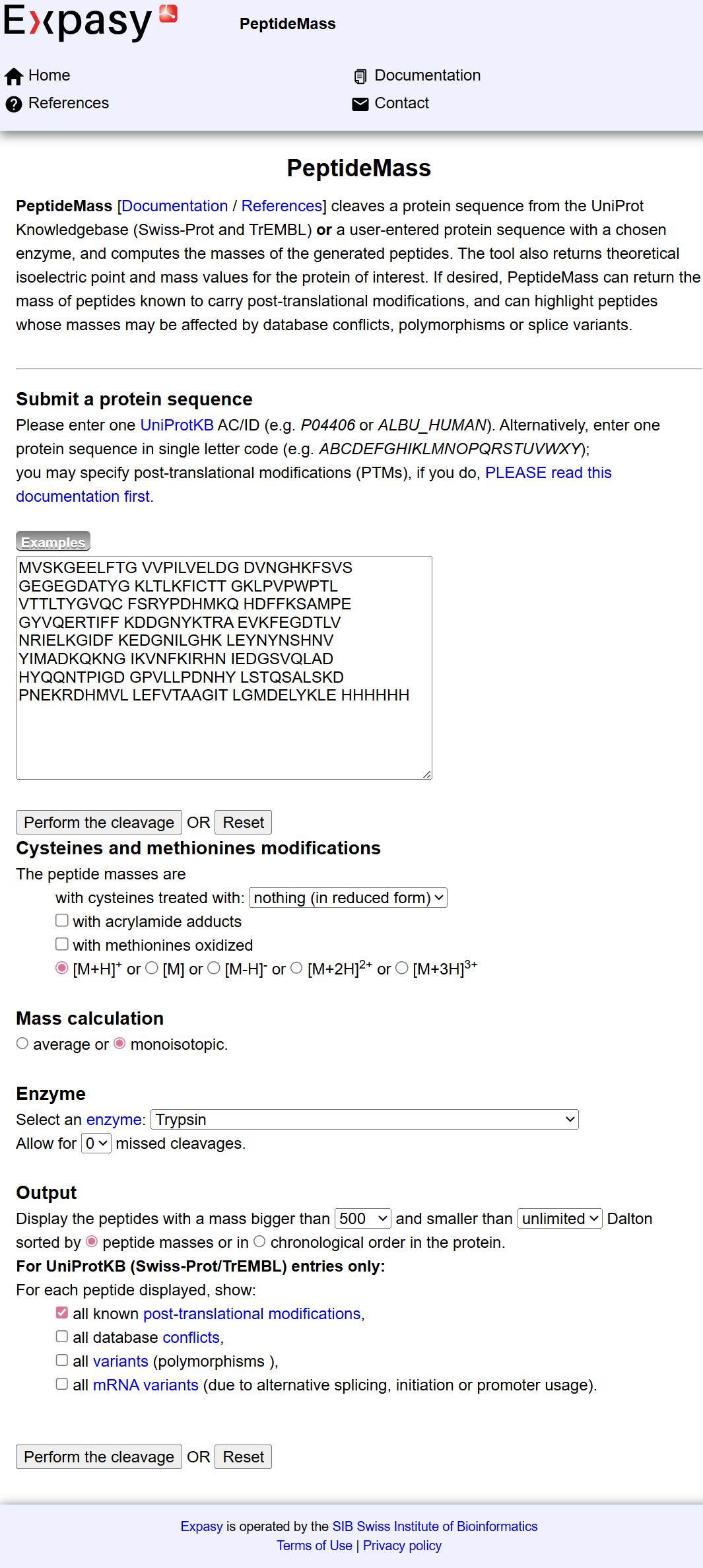
- Navigate to https://web.expasy.org/peptide_mass/
- Copy/paste the sequence above into the input box in the PeptideMass tool to generate expected list of peptides.
- Use Figure 4 below as a guide for the relevant parameters to predict peptides from eGFP.
- Click “Perform the Cleavage” button in the PeptideMass tool and report the number of peptides generated when using trypsin to perform the digest.
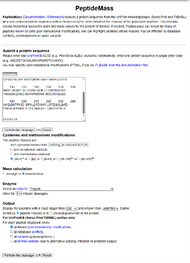 Figure 4. Example conditions for predicting the number of tryptic peptides from the eGFP standard. Please replicate all parameters shown above.
- Based on the LC-MS data for the Peptide Map data generated in lab (please use Figure 5a as a reference) how many chromatographic peaks do you see in the eGFP peptide map between 0.5 and 6 minutes? You may count all peaks that are >10% relative abundance.
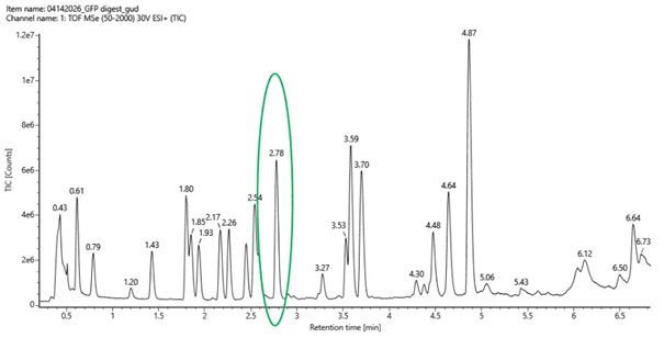 Figure 5a. Total ion chromatogram (TIC) of the eGFP peptide map. The peak at 2.78 minutes is circled, and its MS data is shown in the mass spectrum in Figure 5b, below.
 - Assuming all the peaks are peptides, does the number of peaks match the number of peptides predicted from question 2 above? Are there more peaks in the chromatogram or fewer?
- Identify the mass-to-charge (m/z) of the peptide shown in Figure 5b. What is the charge (z) of the most abundant charge state of the peptide (use the separation of the isotopes to determine the charge state). Calculate the mass of the singly charged form of the peptide (M+H+) based on its m/z and z.
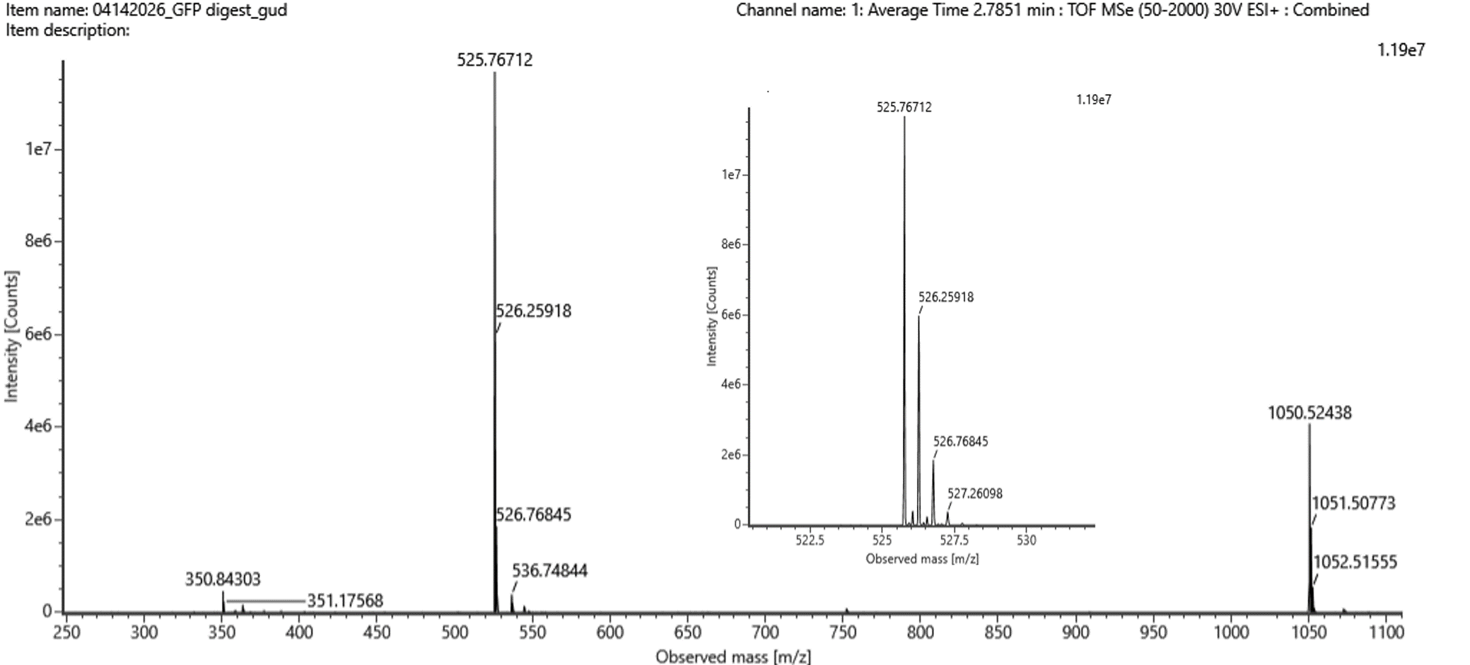 Figure 5b. Mass spectrum figure to show m/zfor the chromatographic peak at 2.78 min from Figure 5a above. The inset is a zoom-in of the peak at 525.76, to discern the isotope peaks.
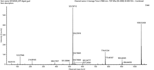 Figure 5c. Fragmentation spectrum of the peptide eluting at retention time 2.78 minutes in Figure 5a (above).
 - Identify the peptide based on comparison to expected masses in the PeptideMass tool. What is mass accuracy of measurement? Please calculate the error in ppm. (Recall that Accuracy = (|Calculated MW – Theoretical MW|) / (Theoretical MW) x 1,000,000 )
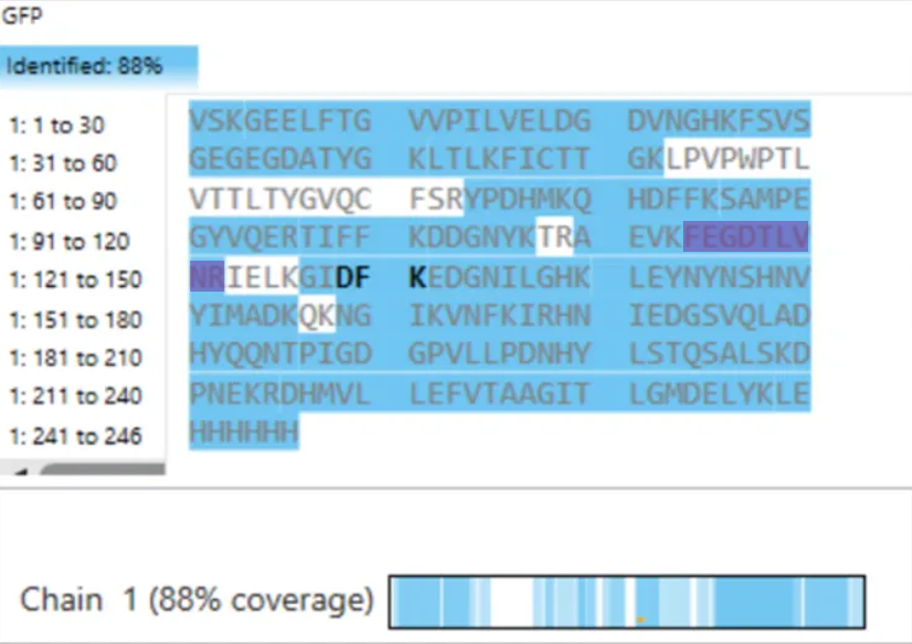
- What is the percentage of the sequence that is confirmed by peptide mapping? (see Figure 6)
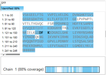 Figure 6. Amino Acid Coverage Map of eGFP based on BioAccord LC-MS peptide identification data.
Bonus Peptide Map Questions
- Can you determine the peptide sequence for the peptide fragmentation spectrum shown in Figure 5c? (HINT: Use your results from Question 2 above to match the peptide molecular weight that is closest to that shown in Figure 5b. Copy and paste its sequence into this tool online to predict the fragmentation pattern based on its amino acid sequence: http://db.systemsbiology.net/proteomicsToolkit/FragIonServlet.html. What is the sequence of the eGFP peptide that best matches the fragmentation spectrum in Figure 5c?
- Does the peptide map data make sense, i.e. do the results indicate the protein is the eGFP standard? Why or why not? Consult with Figure 6, which depicts the % amino acid coverage of peptides positively identified using their calculated mass and fragmentation pattern.
- Identification of Cleavage Sites (K and R residues)
To predict the tryptic digestion pattern of eGFP, I first analyzed the amino acid sequence and counted the number of lysine (K) and arginine (R) residues, since trypsin cleaves specifically after these amino acids.
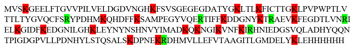 From the sequence analysis:
- Number of Lysine (K): 20
- Number of Arginine (R): 6
- Prediction of Tryptic Peptides
To determine the number of peptides generated after digestion, I used the ExPASy PeptideMass tool by inputting the full eGFP sequence and applying trypsin cleavage conditions.
 The tool predicted a total of: 19 peptides
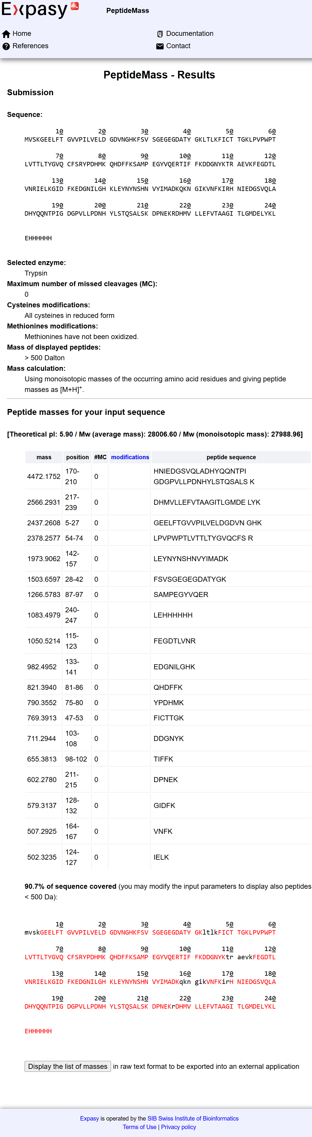
The theoretical molecular weight of eGFP used for reference was: Mw (average mass): 28006.60 Da
- Chromatographic Peak Analysis
From the total ion chromatogram (TIC) shown in Figure 5a, I counted the number of peaks between 0.5 and 6 minutes, considering only peaks with a relative intensity greater than 10%. The number of observed peaks was: 18
- Comparison Between Predicted Peptides and Observed Peaks
The theoretical digestion predicted 19 peptides, while the chromatogram shows 18 peaks. There is slight difference between the theoretical digestion and the chromatogram, but overall, the numbers are very close, indicating good agreement between theoretical prediction and experimental data.
- Peptide Mass and Charge Determination
From Figure 5b, the most abundant peak was observed at: m/z = 525.76
By analyzing the isotope spacing:
- 526.25918 – 525.76712 = 0.49
- 526.76845 - 526.25918 = 0.50
Δm/z ≈ 0.5 → z = 1/ Δm/z = 1/ 0.5 = 2
Thus, the peptide is doubly charged (z=2).
The molecular weight was calculated using:
MW = (m/z x z) – (z x H)
MW = (525.76 x 2) – (2 x 1.0078)
MW = 1049.5044 ≈ 1050
- Peptide Identification
Using the predicted peptide list from the ExPASy tool, I compared the calculated experimental mass (1049.5044 Da) with theoretical peptide masses. The closest match was:
- Peptide sequence: FEGDTLVNR with Theoretical mass: 1050.5214 Da
This confirms that the detected peptide corresponds to this sequence.
Then the mass accuracy was calculated using:
Accuracy = (|Calculated MW – Theoretical MW|) / (Theoretical MW) x 1,000,000
Accuracy = (|1049.5044 – 1050.5214|) / (1050.5214) x 1,000,000
Accuracy = (1.017) / (1050.5214) * 1,000,000
Accuracy = 968.09 ppm > 10
- Sequence Coverage (Figure 6) From the coverage map shown in Figure 6, approximately: 88% of the eGFP sequence was identified This high coverage indicates that most of the protein sequence was successfully confirmed through peptide mapping.
Bonus part:
- Peptide Sequence Confirmation Using Fragmentation
To confirm the identity of the peptide, I used the mass obtained from the LC-MS analysis and matched it with the predicted tryptic peptides. The peptide with the closest theoretical mass was identified as FEGDTLVNR, with a theoretical mass of 1050.52149 Da.
To validate this identification, I used a fragmentation prediction tool to generate the expected b- and y-ion fragments of this peptide.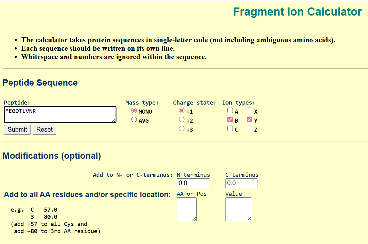 the resulted fragments are as following:
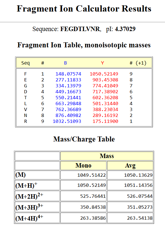
I then compared these predicted fragments with the experimental MS/MS spectrum shown in Figure 5c. Several peaks in the spectrum matched the predicted fragments, especially the y-ions, like :1050.52149; 903.45308; 774.41049; 602.36208, which confirms that the sequence FEGDTLVNR is correct.
The experimental mass of the peptide was 1050.52438 Da, which is very close to the theoretical value. I calculated the mass accuracy using the ppm formula and obtained: accuracy ≈2.75 ppm
This very low error (well below 10 ppm) indicates high measurement accuracy and strong agreement between experimental and theoretical data.
- Sequence Coverage and Protein Confirmation
To evaluate whether the results confirm the identity of the protein, I analyzed the sequence coverage shown in Figure 6. The coverage percentage was approximately 88%, indicating that a large portion of the eGFP sequence was successfully identified.
Additionally, the identified peptide FEGDTLVNR (positions 115–123) is located within the covered regions of the sequence, confirming that this peptide contributes to the overall sequence identification.
 This high sequence coverage, along with the accurate peptide identification and fragmentation matching, confirms that the analyzed protein is indeed eGFP. Although some regions are not covered (likely due to peptides that are too small or poorly ionized), the overall results provide strong confidence in the protein identification.
Homework: Waters Part IV — Oligomers
Assignees for this section
- MIT/Harvard students Required
- Committed Listeners Required
We will determine Keyhole Limpet Hemocyanin (KLH)’s oligomeric states using charge detection mass spectrometry (CDMS). CDMS single-particle measurements of KLH allow us to make direct mass measurements to determine what oligomeric states (that is, how many protein subunits combine) are present in solution. Using the known masses of the polypeptide subunits (Table 1) for KLH, identify where the following oligomeric species are on the spectrum shown below from the CDMS (Figure 7):
- 7FU Decamer
- 8FU Didecamer
- 8FU 3-Decamer
- 8FU 4-Decamer
Polypeptide Subunit Name | Subunit Mass | 7FU | 340 kDa 8FU | 400 kDa Table 1: KLH Subunit Masses
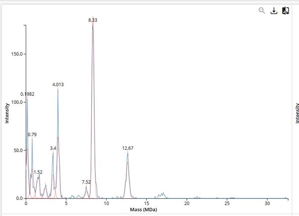 Figure 7. Mass spectrum of Keyhole Limpet Hemocyanin (KLH) acquired on the CDMS.
Oligomer Identification Using CDMS
To determine the oligomeric states of Keyhole Limpet Hemocyanin (KLH), I used the subunit masses provided in Table 1 and calculated the expected total mass for each oligomeric form. The given subunit masses are:
- 7FU = 340 kDa
- 8FU = 400 kDa
Mass Calculations
For each oligomer, the total mass was calculated by multiplying the subunit mass by the number of subunits:
- 7FU Decamer (10 subunits): 10×340 = 3400kDa = 3.4MDa
- 8FU Didecamer (20 subunits): 20×400 = 8000kDa = 8 MDa
- 8FU 3-Decamer (30 subunits): 30×400 = 12000kDa = 12 MDa
- 8FU 4-Decamer (40 subunits): 40×400 = 16000kDa = 16 MDa
Note: While assigning the oligomeric peaks in the CDMS spectrum (Figure 7), I noticed that for the first three oligomers there are clear red peaks, but for the fourth one (~16 MDa), there is only a small blue signal without a corresponding red peak. This made me question why there are two different colors in the spectrum and why the fourth oligomer does not have a red peak.
After looking into this, I understood that the two colors represent different types of data:
- The blue line corresponds to the raw signal detected by the instrument. It includes all detected ions and therefore appears noisy and irregular.
- The red peaks correspond to a fitted model (Gaussian fit) generated by the software. This fit is applied to the raw data to determine the most accurate position (center) of each mass peak.
This means that the red peaks represent the most reliable mass values, while the blue signal shows all detected data, including weaker or less clear signals.
Using this understanding, I assigned the oligomers as follows:
- The peak at 3.4 MDa (red) corresponds to the 7FU decamer
- The peak at 8.33 MDa (red) corresponds to the 8FU didecamer
- The peak at 12.67 MDa (red) corresponds to the 8FU 3-decamer
- For the fourth oligomer (~16.0 MDa), I observed only a small blue “hump” in the region between 16–17 MDa, without any red fitted peak.
This can be explained by the fact that:
- The signal for this oligomer is much weaker compared to the others
- There may be fewer particles detected at this mass
- The signal may be too noisy or not well-defined
Because of this, the software was not able to confidently fit a Gaussian curve, and therefore no red peak was generated. Despite this, the presence of the blue signal at the expected mass range (~16 MDa) still indicates the existence of the 8FU 4-decamer, even if it is less abundant or less stable.
| Parameter | Theoretical | Observed / Measured (Intact LC-MS) | PPM Mass Error |
|---|---|---|---|
| Molecular weight (kDa) | 28.0066 | 27.9829 | 846 |
For this homework, I used AI tools such as ChatGPT and DeepSeek to help structure my ideas and improve the clarity of my writing. I also used NotebookLM to better understand the provided resources and supporting materials. For the final project measurements, DeepSeek suggested including the last four key measurements, which I integrated into my analysis.
Sources:
- EC:1.2.2.4—FACTA Search. (n.d.). Retrieved April 14, 2026, from https://www.nactem.ac.uk/facta/cgi-bin/facta3.cgi?query=EC%3A1.2.2.4%7C111111%7C0%7C0%7C233944%7C0%7C10
- Herminghaus, S., Schreier, P. H., McCarthy, J. E. G., Landsmann, J., Botterman, J., & Berlin, J. (1991). Expression of a bacterial lysine decarboxylase gene and transport of the protein into chloroplasts of transgenic tobacco. Plant Molecular Biology. https://agris.fao.org/search/en/records/65de1eb24c5aef494fd9fee5
- Kim, Y. M., & Hegeman, G. D. (1981a). Purification and some properties of carbon monoxide dehydrogenase from Pseudomonas carboxydohydrogena. Journal of Bacteriology, 148(3), 904–911. https://doi.org/10.1128/jb.148.3.904-911.1981
- Kim, Y. M., & Hegeman, G. D. (1981b). Purification and some properties of carbon monoxide dehydrogenase from Pseudomonas carboxydohydrogena. Journal of Bacteriology, 148(3), 904–911. https://doi.org/10.1128/jb.148.3.904-911.1981
- Matzke, M. A., & Matzke, A. J. (1998). Epigenetic silencing of plant transgenes as a consequence of diverse cellular defence responses. Cellular and Molecular Life Sciences: CMLS, 54(1), 94–103. https://doi.org/10.1007/s000180050128
- Maxwell, K., & Johnson, G. N. (2000). Chlorophyll fluorescence—A practical guide. Journal of Experimental Botany, 51(345), 659–668. https://doi.org/10.1093/jxb/51.345.659
- Pahlow, S., Ostendorp, A., Krü, L., ß, el, & Kehr, J. (2018). Phloem Sap Sampling from Brassica napus for 3D-PAGE of Protein and Ribonucleoprotein Complexes. JoVE (Journal of Visualized Experiments), (131), e57097. https://doi.org/10.3791/57097
- Recent Advances and Emerging Trends in Chlorophyll Fluorescence Parameter Fv/Fm. (2025). Phyton-International Journal of Experimental Botany, 94(9), 2615–2630. https://doi.org/10.32604/phyton.2025.069246
- Remelli, W., Villafiorita, F., Casazza, A. P., & Santabarbara, S. (2018). Comparative excitation-emission dependence of the FV/FM ratio in model green algae and cyanobacterial strains. https://iris.cnr.it/handle/20.500.14243/365902
- Schägger, H., & von Jagow, G. (1991). Blue native electrophoresis for isolation of membrane protein complexes in enzymatically active form. Analytical Biochemistry, 199(2), 223–231. https://doi.org/10.1016/0003-2697(91)90094-a
- Smith, P. K., Krohn, R. I., Hermanson, G. T., Mallia, A. K., Gartner, F. H., Provenzano, M. D., Fujimoto, E. K., Goeke, N. M., Olson, B. J., & Klenk, D. C. (1985). Measurement of protein using bicinchoninic acid. Analytical Biochemistry, 150(1), 76–85. https://doi.org/10.1016/0003-2697(85)90442-7
- Woo, J.-K., Hong, C. B., & Lee, J.-S. (1991). Chloroplast Targeting of Bacterial β-Glucuronidase with a Pea Transit Peptide in Transgenic Tobacco Plants. Molecules and Cells, 1(4), 451–457. https://doi.org/10.1016/S1016-8478(23)13893-3