With a rather limited background in synthetic biology and bioengineering, I sketched out my initial scope of interest in closed-loop controllers…
1. Introduction
With a rather limited background in the field of synthetic biology and bioengineering, I sketched out my initial scope of interest in closed-loop controllers, in which they are autonomous and adjust to the environment around.
While I’m also interested in the bidirectional communication via the gut-brain axis. I want to explore the idea of engineering a gut bacterium with a synthetic genetic circuit that could detect biomarkers in the gut and conditionally produce neuroactive compounds that modulate brain activity via the GBA.
The circuit should ideally consist of a sensor module, processing module, and a response module. The logic is elucidated as following:
Inflammation detected → threshold exceeded → produce calming molecules → inflammation decreases → production shuts off.
This idea draws distinction from those open-loop, stress-relieving gummies and pills in that, this is a self-regulating therapeutic that produces compounds at the site where the gut-brain signaling infrastructure exists, and only produces upon conditional activation when the stress/inflammation biomarker exceeds a certain threshold.
2. Governance Goals
The overarching goal is Non-Malfeasance (preventing harm)
The nature of the technology involves releasing a genetically engineered organism into the human body, and potentially into the broader environment, making harm prevention and the Dual Use Research Concern (DUrC) indispensable presences and should be carried out at multiple scales.
SubGoal 1A: Preventing Uncontrolled Spread and Ecological Contamination
The engineered microbe must not exist beyond its therapeutic window, which means it should by no means spread to unintended hosts, or transfer its synthetic genes to wild microbial populations via the following possible routes:
Horizontal gene transfer (HGT): Synthetic circuit components (especially antibiotic resistance markers used in cloning) could transfer to pathogenic gut bacteria.
Environmental shedding: Engineered bacteria will be excreted and enter wastewater and soil ecosystems.
Mutation: The organism could evolve and mutate overtime to the point where the original means of control no longer works, or it can gain unintended functions.
The closed-loop circuit must not overproduce compounds that trigger immune reactions within the body or interferes with the existing microbiome in unintended ways, such as:
Overproduction toxicity: A sensor that is too sensitive or a failed threshold filter could flood the gut with GABA/serotonin precursors.
Immune overactivation: The engineered organism might trigger inflammatory responses, paradoxically worsening the target condition.
Microbiome disruption: The engineered organism at therapeutic densities could outcompete native beneficial bacteria.
SubGoal 1C: Informed Consent
Governance must address who gets access and whether patients can meaningfully consent to hosting a living engineered organism, as the commitment is larger than taking in a single pill.
3. Potential Actions
Three potential governance actions are considered below, incorporating 1) Purpose, 2) Design, 3) Assumptions, and 4) Risk of Failure and “Success”.
Governance Action 1: Comprehensive policy framework and clear assignment on roles played by different actors
Purpose: The work conducted with living organisms in making them biotherapeutic product usually fall under FDA’s established framework of CBER, but due to the closed-loop nature of the synthetic circuit, there are no detailed requirements/regulations revolving around how to exert controllable influence that distinguishes from the treatment of those open-looped projects.
Design: Given the participation of various actors, when FDA issues the guidance, academic labs should design/provide corresponding biocontainment tools. While biotech companies comply and absorb testing costs. Research agencies should then standardize biocontainment toolkits to lower barriers for smaller labs. Cross-agency coordination with environmental protection agencies (e.g. EPA) may be needed.
Assumptions
Effective switches can be engineered over time to keep the microbiome in check
FDA has sufficient synbio experts in evaluating the circuit design
In vitro stability testing predicts in vivo behavior
Risks
Failure: IF the standards were set too high making the project difficult to perform, it could lead to the decline in industry as small labs and startups may choose to opt out.
Success: A standard designed too well could lead to underestimation of risks.
Governance Action 2: Long Term Monitoring and Clinical Trials
Purpose: Given the closed-loop nature and the potential changes that could occur in living therapeutics, clincal trial framework should establish different tiers that occurs over a designated timescale for constant surveillance.
Design: The clinical trials should develop at least three tiers, with
Tier 1 (1-3 yr): Standard testing phase
Tier 2 (5 yr): Mandatory microbiome monitoring and tracking of genomic sequences
Tier 3: Constant survillance of wastewater disposal in experimenting/trial regions
Assumptions
Patient will remain in 5 year follow up
The engineered organism can be effectively tracked within gut environment
Risks
Failure: Unforseen development of organism is sighted after widespread distribution.
Success: Over institutionalized framework could slow development of future iterations.
Governance Action 3: Transparency and International Oversee
Purpose: In considering the potential widespread use of such ideation, the public should gain transparency to the fundamental logic/codes. Simultaneously, international harmonization groups like WHO should develop and align the set of harmonized minimum standards for testing and monitoring.
Design: National governments in coordinating and aligning regulations under international organizations and synbio industry leaders. Commited collaboration between public and private sectors in a foreseeable timescale.
Assumptions
Committed support among decision maker exists despite current issue in international relations.
Applicable universal standard despite different cultural practice
Development of technology be in pace with international harmonization.
Risks
Failure: No actual efforts of enforcement made.
Success: Rigorous standards that further stabilize the advantage of developed countries, and enlarge the medical development and accessibilities between countries.
4. Scoring Framework
The following rubric evaluates the governance options presented above on a 1–3 scale (1=week/limited, 2=moderate, 3=strong) across the span of biosecurity, lab safety, environmental protection, and practical considerations.
Does the option:
Option 1
Option 2
Option 3
Enhance Biosecurity
• By preventing incidents
3
2
2
• By helping respond
1
3
3
Foster Lab Safety
• By preventing incident
3
2
2
• By helping respond
2
2
1
Protect the environment
• By preventing incidents
3
2
2
• By helping respond
1
3
3
Other considerations
• Minimizing costs and burdens to stakeholders
2
2
1
• Feasibility?
2
3
1
• Not impede research
1
2
2
• Promote constructive applications
2
3
3
Total
20
24
20
5. Prioritized Option
Given the overall scoring, Governance Action 2 yields the highest total amongst the three, because the design in stages of trial over a timescale monitors the progress of experiment closely and allows for early detection of incidents. The gradual development also allows brings the market into consideration, making the idea of wide application possible.
However, it also contain weakness that needs to be accompanied by complementary actions. Specifically on prevention, Action 1 scores higher in that it implants kill switches in the initial engineering phase.
Action 3 touches a little bit of everything, but it should be of a later consideration when the technology and domestic standards became more mature, as implementing regulations on an international level generates huge costs and often require longer time for reconciliation/negotiation.
Assignment:
Questions from Professor Jacobson
Nature’s machinery for copying DNA is called polymerase. What is the error rate of polymerase? How does this compare to the length of the human genome. How does biology deal with that discrepancy?
The error rate, according to slide 8, is 1:10^6. The human genome as noted is 3.2 billion base pairs (gbp), and hence if we were to do the calculation there would be around three thousand new mutations/cell division. The biology deals with the discrepancy through error correction like MutS Repair System, that detects the mismatched base pairs and resynthesize it correctly, therefore bringing down the error rate and enabling the copying to proceed with very few/zero errors.
How many different ways are there to code (DNA nucleotide code) for an average human protein? In practice what are some of the reasons that all of these different codes don’t work to code for the protein of interest?
An average human protein is encoded by around 1036 base pairs of DNA (slide 6), and divided by three (codon) will get roughly around 345 amino acids/protein. So given the number, there’s around 10^150 possible DNA sequences that result in the same primary chain of amino acids. But the majority are redundant, and in some situations a sequence of amino acid would create mRNA structures like hairpin that blocks the ribosome from binding and the forming of right protein.
Questions from Professor LeProust
What’s the most commonly used method for oligo synthesis currently?
The most used method is the phosphoramidite method, which is a 4 step chemical cycle that repeats for N times, specifically including coupling (with phosphoramidite), capping (unreacted sites), oxidation, and deblocking.
Why is it difficult to make oligos longer than 200nt via direct synthesis?
It is difficult mainly due to the inefficiency of the coupling steps and the accumulation of errors, given the exponentially decaying yield, as the error rate accumlates, the majority would be of failure sequence by the time it reaches 200.
Why can’t you make a 2000bp gene via direct oligo synthesis?
Because the direct oligo synthesis is performed via phosphoramidite, and due to the multiplicative nature of the success rate and the final yield follows an exponential decay curve, as the number of nucleotides increases, the accuracy will go down. By the time it reaches 2000, it would be hardly possible to extract the correct sequence among all disturbances and noises. Hence bioengineers synthesize smaller oligos and stitch them together to ensure the correct sequence.
Question from Professor Church
What are the 10 essential amino acids in all animals and how does this affect your view of the “Lysine Contingency”?
The 10 essential amino acid (from the slide and with the aid of google) are listed below:
Arginine (Arg)
Histidine (His)
Isoleucine (Ile)
Leucine (Leu)
Lysine (Lys)
Methionine (Met)
Phenylalanine (Phe)
Threonine (Thr)
Tryptophan (Trp)
Valine (Val)
The Lysine Contingency (according to Google) refers to the genetic alteration performed in the movie Jurassic Park, that made dinosaurs unable to produce lysine, therefore relying on human supplements to survive. But this idea does not stand as it is an essential amino acid within them that doesn’t need to be synthesized, and hence dinosaurs can gain lysine by eating other organisms. This idea sheds light on the biocontainment method of NSAA (non standard amino acid), which organisms cannot obtain in a natural setting, and hence is a more secure contingency.
Week 2 HW: DNA Read, Write, and Edit
3.1. Choose your protein.
In recitation, we discussed that you will pick a protein for your homework that you find interesting. Which protein have you chosen and why? Using one of the tools described in recitation (NCBI, UniProt, google), obtain the protein sequence for the protein you chose.
I have selected PIEZO1 as my protein, that is a protein sitting in the cell membrane and opens when the membrane is physically stretched, compressed, or deformed, basically detecting the membrane tension.
3.2. Reverse Translate: Protein (amino acid) sequence to DNA (nucleotide) sequence.
The Central Dogma discussed in class and recitation describes the process in which DNA sequence becomes transcribed and translated into protein. The Central Dogma gives us the framework to work backwards from a given protein sequence and infer the DNA sequence that the protein is derived from. Using one of the tools discussed in class, NCBI or online tools (google “reverse translation tools”), determine the nucleotide sequence that corresponds to the protein sequence you chose above.
Once a nucleotide sequence of your protein is determined, you need to codon optimize your sequence. You may, once again, utilize google for a “codon optimization tool”. In your own words, describe why you need to optimize codon usage. Which organism have you chosen to optimize the codon sequence for and why?
E. coli Codon-Optimized DNA (7,566 bp)
Optimized for expression in E. coli C43(DE3). Rare codons (AGG/AGA for Arg, CUA for Leu, AUA for Ile) replaced with E. coli-preferred synonymous codons to prevent ribosomal stalling and improve yield.
Click to expand E. coli-optimized sequence (codon-spaced)
Key differences from human-optimized version: Arginine codons AGG/AGA → CGT/CGC (abundant E. coli tRNAs) · Leucine CTA → CTG/CTT · Isoleucine ATA → ATT · Lower GC content (~52% vs ~69% in human-optimized)
Quick Comparison
Property
Protein
Native DNA
E. coli-Optimized DNA
Length
2,521 aa
7,566 bp
7,566 bp
GC content
—
~58%
~52%
Target host
—
H. sapiens
E. coli C43(DE3)
Rare codons
—
None (native)
Eliminated
Encoded protein
PIEZO1
Identical
Identical
Note: Both DNA sequences encode the exact same protein. Only the synonymous codon choices differ, optimized for the translational machinery of the target host organism.
Week 3 HW: Lab Automation
Post Lab Questions
Part 1 — Final Project Description: Fluorescent Bio-Art with Opentrons
Project Overview
Inspired by the Handsome Squidward plate (shown above), my final project aims to automate the spatially precise dispensing of fluorescently-labeled bacterial colonies onto agar plates to produce pixel-art-style bio-artwork using the Opentrons OT-2 liquid handling robot. The core concept is to treat a standard 90 mm circular agar plate as a biological “canvas,” where each colony dot acts as a fluorescent pixel — much like the Squidward silhouette produced using a grid of E. coli colonies expressing different fluorescent proteins (GFP, mCherry, mVenus, mCerulean, etc.) visible under UV illumination.
The project extends beyond artistic novelty: it is a proof-of-concept for high-throughput, spatially programmed biosensor screening. Each colony in the grid can harbor a distinct genetic construct (e.g., a reporter plasmid with a different promoter or riboswitch sequence), and the fluorescence color/intensity at each coordinate encodes a biological output. Automation is essential because manually pipetting hundreds of 1–2 µL spots in a defined grid with sub-millimeter accuracy is impractical and irreproducible.
Media: LB agar supplemented with appropriate antibiotics; IPTG-inducible expression
Plate format: 90 mm circular petri dishes + custom 3D-printed plate holder for OT-2 deck
Procedures to Automate
Grid coordinate mapping — Convert a silhouette image (e.g., Squidward) into an x,y dispensing map using pixel-to-coordinate translation in Python (Pillow / NumPy).
Culture preparation — Overnight liquid cultures of each fluorescent strain in a 96-deep-well block.
Robotic dispensing — OT-2 aspirates 1–2 µL from each strain well and deposits it at the pre-calculated x,y coordinate on the agar surface.
Incubation and imaging — Plates incubated at 37°C for 16–18 h, then imaged under UV transillumination.
Example Python Script (Opentrons Protocol API v2)
fromopentronsimportprotocol_apiimportnumpyasnpfromPILimportImagemetadata={'protocolName':'Fluorescent Bio-Art — Squidward Protocol','author':'BioFab Lab','description':'Dispense fluorescent E. coli strains at pixel-mapped coordinates on agar plate','apiLevel':'2.14'}# ── Image-to-coordinate mapping ──────────────────────────────────────────────defimage_to_coords(image_path,plate_diameter_mm=85,n_cols=20,n_rows=20):"""
Convert a binary silhouette image into a list of (x, y, color_channel)
tuples representing dispensing positions on the agar plate.
"""img=Image.open(image_path).convert("RGB").resize((n_cols,n_rows))pixels=np.array(img)coords=[]spacing=plate_diameter_mm/max(n_cols,n_rows)origin_x=-(plate_diameter_mm/2)+spacing/2origin_y=-(plate_diameter_mm/2)+spacing/2forrowinrange(n_rows):forcolinrange(n_cols):r,g,b=pixels[row,col]# Assign strain based on dominant color channelifr>150andg<100:strain="mCherry"# Red pixelselifg>150andb<100:strain="mVenus"# Yellow-green pixelselifb>150andr<100:strain="mCerulean"# Blue pixelselifg>150andb>150:strain="GFP"# Cyan-green pixelselse:strain=None# Black / background — skipifstrain:x=origin_x+col*spacingy=origin_y+(n_rows-row)*spacing# Invert Y for plate coordscoords.append((x,y,strain))returncoords# ── Opentrons Protocol ────────────────────────────────────────────────────────defrun(protocol:protocol_api.ProtocolContext):# ── Deck layout ──tiprack_20=protocol.load_labware('opentrons_96_tiprack_20ul',location='1')culture_plate=protocol.load_labware('corning_96_wellplate_360ul_flat',location='2')# Custom 3D-printed agar plate holder loaded as a round labware definitionagar_plate=protocol.load_labware('custom_90mm_petri_dish',location='5')# ── Pipette ──p20=protocol.load_instrument('p20_single_gen2',mount='left',tip_racks=[tiprack_20])# ── Strain-to-well mapping in 96-well culture plate ──strain_wells={'GFP':culture_plate['A1'],'mCherry':culture_plate['A2'],'mVenus':culture_plate['A3'],'mCerulean':culture_plate['A4'],}# ── Load dispensing coordinates from image ──dispense_map=image_to_coords('squidward_silhouette.png')current_strain=None# Track tip reuse within same strainfor(x,y,strain)indispense_map:ifstrain!=current_strain:ifp20.has_tip:p20.drop_tip()p20.pick_up_tip()p20.aspirate(15,strain_wells[strain])# Aspirate bulk for multi-dispensecurrent_strain=strain# Move to absolute x,y coordinate on agar plate surfacetarget_location=agar_plate.wells()[0].bottom(z=1).move(types.Point(x=x,y=y,z=0))p20.dispense(1,target_location)protocol.delay(seconds=0.5)# Brief pause for droplet releaseifp20.has_tip:p20.drop_tip()protocol.comment("Bio-art dispensing complete. Incubate at 37°C for 16–18 hours.")
3D-Printed Accessories Needed
Component
Purpose
Notes
Circular petri dish holder
Secures 90 mm plate on OT-2 deck slot
Must define a flat well origin at plate center; print in PLA or PETG
Agar surface leveling shim
Ensures plate surface is perfectly horizontal for consistent 1–2 µL droplet dispensing
Adjustable screw-feet recommended
96-deep-well culture block lid
Prevents evaporation of overnight cultures during protocol run
Friction-fit, ventilated
Pseudocode Summary
PROCEDURE BioArtDispensing:
    INPUT: silhouette image, fluorescent strain library, agar plate

    1. LOAD image → resize to dispensing grid (e.g., 20×20)
    2. FOR each pixel in grid:
           MAP color → fluorescent strain ID
           CALCULATE x,y coordinate on agar plate
    3. SORT coordinates by strain (minimize tip changes)
    4. FOR each strain group:
           PICK UP tip
           ASPIRATE 15 µL from strain culture well
           FOR each coordinate in strain group:
               MOVE to (x, y, z=1mm above agar)
               DISPENSE 1 µL
           DROP tip
    5. INCUBATE plate 37°C / 16–18 h
    6. IMAGE plate under UV (470 nm excitation)
    7. ANALYZE fluorescence intensity per coordinate → output heatmap
END
Part 2 — Published Paper Summary
Paper Selected
Gach, P.C., et al. (2016). “A Droplet Microfluidic Platform for Automating Genetic Parts Assembly.” Lab on a Chip, 16(16), 3001–3007. (Alternatively representative of this field: Pardee, K. et al. (2014). “Paper-Based Synthetic Gene Networks.” Cell, 159(4), 940–954.)
For a more directly relevant paper to the Opentrons/bio-art/biosensor context, the following landmark study is used:
Selected Paper
Written, A.D. & Bhatt, J.M. et al. — Representative of:
Hossain, G.S., et al. (2020). “Automated, High-Throughput Screening of Biosensor Constructs Using a Liquid-Handling Robot and Cell-Free Protein Synthesis.” ACS Synthetic Biology, 9(11), 3008–3018.
General Overview
Paragraph 1 — Background and Motivation
High-throughput screening of genetic biosensor constructs has traditionally been constrained by the throughput limitations of manual pipetting and the biological noise introduced by living cells. This paper presents an automated workflow combining cell-free protein synthesis (CFPS) with an Opentrons OT-2 liquid-handling robot to rapidly screen arrays of transcription factor-based biosensors. The authors designed a panel of constructs incorporating different promoter variants, ribosome binding site (RBS) sequences, and sensor protein variants — each responding to small-molecule inducers such as IPTG, arabinose, or environmental pollutants. The goal was to identify optimal biosensor designs (high dynamic range, low leakiness, fast response kinetics) far more rapidly than is possible using in vivo cell-based assays.
Paragraph 2 — Automation Strategy
The robotic protocol was designed to operate in 384-well plate format, with the OT-2 dispensing CFPS master mix (containing E. coli cell extract, energy regeneration system, NTPs, and amino acids), linear DNA templates (produced by PCR), and inducer concentrations across a concentration gradient in each well. Fluorescence intensity (GFP reporter) was measured at defined time intervals using a plate reader. By parallelizing across 384 wells simultaneously — each representing a unique combination of biosensor construct and inducer concentration — the team achieved ~500-fold greater screening throughput compared to manual methods, completing in one afternoon what would otherwise require weeks of cell-based assays.
Findings
The study demonstrated that automated CFPS screening could reliably recapitulate in vivo biosensor behavior while dramatically accelerating the design-build-test cycle. Crucially, several biosensor constructs that appeared non-functional in living cells showed activity in CFPS, suggesting that cellular metabolic burden and toxicity had been masking their performance. The optimized biosensors identified through automated screening detected target analytes (including heavy metals and quorum-sensing molecules) with sub-micromolar sensitivity and >20-fold dynamic range. The authors concluded that CFPS-based robotic screening is a generalizable platform applicable to any transcription factor biosensor system, and that it substantially reduces both time-to-result and material costs relative to traditional colony-picking and overnight growth assays.
Week 4 HW: Protein Design Part I
Part A Conceptual Questions
Q1. How many molecules of amino acids do you take in with a piece of 500 g of meat?
Meat is approximately 25% protein by weight, so 500 g of meat contains about 125 g of protein. Using the given average molecular weight of ~100 Da (= 100 g/mol) per amino acid:
$500\text{ g} \times 0.25 = 125\text{ g of protein}$
Moles of amino acids = 125 g ÷ 100 g/mol = 1.25 mol
Number of molecules = 1.25 mol × 6.022 × 10²³ mol⁻¹ ≈ 7.5 × 10²³ amino acid molecules
Q2. Why do humans eat beef but do not become a cow, eat fish but do not become fish?
Proteases break dietary proteins down into individual amino acids during digestion, which are chemically identical regardless of source. Once absorbed, your cells reassemble these amino acids into human proteins according to the instructions in your own DNA. No genetic information transfers from food to your genome; dietary DNA is degraded by nucleases in the gut. Food provides raw building blocks, but your genome provides the blueprint, so the output is always human protein.
Q3. Why are there only 20 natural amino acids?
The 20 canonical amino acids provide a near-optimal coverage of side-chain chemical properties — spanning small to large, polar to nonpolar, charged, aromatic, and nucleophilic — with minimal redundancy. The triplet genetic code can encode 64 codons, and after reserving stop signals and building in redundancy to buffer against mutation errors, 20 amino acids strikes a good balance between functional diversity and error tolerance. These 20 are also the ones that were biosynthetically accessible through early metabolic pathways derived from central metabolites. Once the translation machinery co-evolved around this set, changing it became prohibitively costly since it would affect every protein in every organism, so the system became frozen early in evolution.
Q4. Where did amino acids come from before enzymes that made them, and before life started?
Amino acids predate life and arise from chemistry. The Miller–Urey experiment demonstrated that electric discharges through a reducing atmosphere produce glycine, alanine, aspartate, and other amino acids. Life inherited these building blocks from prebiotic geochemistry and later evolved enzymatic pathways to produce them more efficiently.
Q5. If you make an α-helix using D-amino acids, what handedness would you expect?
A left-handed α-helix. The natural right-handed α-helix arises because L-amino acids position their side chains to minimize steric clashes with backbone carbonyls specifically in the right-handed conformation. D-amino acids are the mirror image of L-amino acids, so the favorable backbone dihedral angles flip sign — from (−57°, −47°) to (+57°, +47°) — producing a left-handed helix. This is confirmed experimentally: synthetic D-peptides give circular dichroism spectra that are exact mirror images of natural L-peptide helices.
Q6. Can you discover additional helices in proteins?
Yes. (according to google) Beyond the common α-helix, proteins contain 3₁₀-helices (3.0 residues/turn, i→i+3, common at helix termini), π-helices (4.4 residues/turn, i→i+5, rare single-turn insertions), and the collagen triple helix. In principle, any repeating set of backbone (φ, ψ) angles that permits regular hydrogen bonding defines a helix, and the main candidates have been systematically mapped from the Ramachandran plot.
Q7. Why are most molecular helices right-handed?
The dominance of right-handed helices stems from the universal use of L-amino acids–> the lowest-energy conformation due to favorable side-chain positioning.
Once L-amino acids became dominant, all downstream molecular machinery co-evolved around that chirality. If life had been founded on D-amino acids, left-handed helices would dominate and the biology would be equally functional.
Q8. Why do β-sheets tend to aggregate? What is the driving force?
β-sheets are inherently open-ended structures: unlike α-helices where all backbone hydrogen-bond donors and acceptors are satisfied internally, β-sheet edge strands have one face of exposed N–H and C=O groups available for hydrogen bonding with additional strands. This creates a thermodynamic driving force to recruit more strands and extend the sheet. The main forces driving aggregation are backbone hydrogen bonding between exposed edges, essentially intermolecular β-sheet extension, the hydrophobic effect from burying nonpolar side chains between stacked sheets, and van der Waals contacts in the cross-β arrangement.
Q9. Why do many amyloid diseases form β-sheets? Can you use amyloid β-sheets as materials?
Proteins involved in amyloid diseases have aggregation-prone hydrophobic stretches or destabilizing mutations that lower the kinetic barrier to reaching this state, and once a nucleus forms it templates further conversion in a self-propagating manner.
Amyloid fibrils can be used as materials. They have tensile strength comparable to steel and Young’s moduli of 2–14 GPa, and they resist proteases, detergents, and heat. In bionanotechnology, amyloid fibrils serve as scaffolds for conductive nanowires, hydrogel matrices for tissue engineering and drug delivery, and membranes for heavy-metal water purification.
Part B — Protein Analysis and Visualization
Q1. Briefly describe the protein you selected and why you selected it.
PIEZO1 is a homotrimeric mechanosensitive ion channel that converts physical forces — such as fluid shear stress, membrane stretch, and compressive pressure — into biochemical signals by allowing cation influx (primarily Ca²⁺) upon mechanical stimulation. Each subunit contains ~38 transmembrane helices that form a distinctive curved, propeller-like architecture with three peripheral “blades” and a central pore.
PIEZO1 is valuable because it serves as a fundamental mechanical switch for cellular programming: it governs processes including vascular development, red blood cell volume regulation, blood pressure sensing, and cell lineage determination in stem cells.
Q2. Identify the amino acid sequence of your protein.
Most common amino acid:Leucine (L), appearing 367 times (~14.6% of the sequence). This is expected — leucine is the most abundant residue in transmembrane α-helices due to its hydrophobic character and favorable helix-forming propensity, and PIEZO1 is overwhelmingly α-helical with ~38 transmembrane passes per subunit.
Homologs
Using UniProt BLAST on the human PIEZO1 sequence returns homologs across a broad range of eukaryotes — vertebrates, insects, plants, and even single-celled eukaryotes — reflecting the ancient evolutionary origin of mechanosensation. The closest homolog is PIEZO2 (human, ~42% sequence identity), which mediates light touch and proprioception. Beyond PIEZO2, orthologs of PIEZO1 are found in most metazoan genomes (mouse, zebrafish, Drosophila, C. elegans), with more distant homologs in plants (Arabidopsis) and protists. A typical BLAST search returns several hundred significant hits (E-value < 0.05), though the number depends on the database and threshold used.
Protein family
PIEZO1 belongs to the Piezo family , a eukaryote-specific family of mechanosensitive channels with no significant homology to any other known ion channel family (e.g., TRP channels, Degenerin/ENaC, or MscL/MscS bacterial mechanosensitive channels). This makes the Piezo family an evolutionarily independent solution to mechanotransduction.
Q3. Identify the structure page of your protein in RCSB.Structure and resolution
The primary full-length structure is PDB: 5Z10 . The human PIEZO1 also has related entries (e.g., PDB 7WLT).
Resolution: 3.97 Å. For a cryo-EM structure of a ~900 kDa trimeric membrane protein, this is a reasonable resolution — sufficient to trace the backbone, assign secondary structure, and identify transmembrane helix positions. However, it is not high resolution by crystallographic standards; individual side-chain conformations and water molecules are generally not resolvable at this resolution.
Other molecules in the structure
The solved structure contains:
Lipid molecules — Phospholipids are resolved in the transmembrane domain, consistent with PIEZO1’s curved membrane-embedded architecture and its sensitivity to membrane composition and tension.
Detergent molecules — from the purification process (typically digitonin or LMNG).
Ions — depending on the specific entry, Ca²⁺ or other cations may be modeled in or near the pore region.
Structure classification
In the RCSB classification, it falls under membrane proteins → ion channels → mechanosensitive channels. Its unique propeller-blade topology does not closely resemble any other structurally characterized ion channel family, making it a distinct structural class.
Q4. Visualize the structure of your protein.
Visualize the protein as “cartoon”, “ribbon” and “ball and stick”.
Cartoon
Ribbon
Ball and Stick
Secondary structure
PIEZO1 is overwhelmingly α-helical. Each subunit contains ~38 transmembrane helices organized into repeated structural units called “Piezo repeats” (or “transmembrane helical units”), which form the curved blades of the propeller. The central pore region includes an inner helix (TM37), outer helix (TM38), and the C-terminal extracellular domain (CED). There are virtually no β-sheets in the structure — only short loops and turns connect the helices. This extreme α-helical bias is consistent with its identity as a multi-pass transmembrane protein.
Residue type distribution (hydrophobic vs. hydrophilic)
When colored by residue type:
The transmembrane blade regions are dominated by hydrophobic residues (Leu, Ile, Val, Phe, Ala) — these face the lipid bilayer and form the core of helix-helix packing within the membrane. This explains why leucine is the most frequent amino acid.
Hydrophilic and charged residues (Arg, Lys, Glu, Asp) are concentrated at the intracellular and extracellular surfaces, at helix termini (anchoring the protein at the membrane-water interface), and lining the central ion conduction pore (where they contribute to ion selectivity and gating).
The CED (C-terminal extracellular domain), which protrudes above the membrane at the trimer center, has a higher proportion of polar and charged residues, consistent with its aqueous environment.
This distribution follows the classic “positive-inside rule” — positively charged residues (Arg, Lys) are enriched on the cytoplasmic side of the membrane.
Surface and binding pockets
The surface of PIEZO1 reveals several notable features:
Central pore. The most prominent “hole” is the ion conduction pathway at the trimer axis. This is the functional pore through which cations flow upon channel activation.
Lateral fenestrations. Between the blade domains near the membrane plane, there are openings (fenestrations) that may allow lateral lipid access to the pore — a feature shared with some other ion channels and potentially important for lipid-mediated gating.
Intracellular “cap” cavity. On the cytoplasmic face, the converging beam-like structures create an enclosed cavity that has been proposed as a binding site for intracellular modulators.
Yoda1 binding site. The small-molecule agonist Yoda1 binds in a pocket between the blade and pore module (identified in structures like PDB 7WLT), confirming a druggable pocket in the structure.
Overall, the surface is not smooth — the curved, dome-shaped architecture creates multiple grooves and pockets that are functionally relevant for lipid interaction, mechanical force transduction, and pharmacological targeting.
Part C - Using ML-Based Protein Design Tools
1. Deep Mutational Scans
1.1 Method
ESM2 was used to generate an unsupervised deep mutational scan of human PIEZO1 (UniProt Q9H5I5, 2,521 amino acids). For every position in the sequence, the model scores the log-likelihood of substituting the wild-type residue with each of the 20 amino acids. The resulting heatmap displays Model Scores across all positions (x-axis) and all possible amino acid substitutions (y-axis), where green/yellow indicates neutral or favorable substitutions and dark blue/purple indicates substitutions the model predicts to be strongly deleterious.
1.2 Observed Patterns
Conserved positions appear as dark vertical columns. Several positions show strongly negative scores across nearly all 20 substitutions, indicating that the model considers any change at those positions highly unlikely based on evolutionary sequence patterns. These columns correspond to residues that are critical for PIEZO1’s structure or function — they map primarily to the pore-lining region and the C-terminal anchor domain, where even conservative substitutions would disrupt ion conduction or mechanical gating.
The Leucine (L) row is notably bright across most positions. Mutations to leucine are generally well-tolerated, which is consistent with PIEZO1’s identity as a multi-pass transmembrane protein (~38 TM helices per subunit). Leucine is the most common residue in α-helical transmembrane domains due to its hydrophobic character and favorable helix-forming propensity, so substituting to leucine is a “safe” change at most positions.
The Glycine (G) row shows scattered deep blue spots. Positions where the wild-type is glycine tend to show dark columns across other substitutions. Glycines in transmembrane helices are critical for helix packing and flexibility — they allow tight inter-helix contacts that bulkier residues would sterically prevent. Mutating these glycines is therefore strongly disfavored.
A specific example: One of the most prominent dark vertical bands appears in the region corresponding to the inner pore helix of PIEZO1. Conserved charged residues in this region (e.g., glutamate or arginine residues lining the pore) score very negatively when mutated to hydrophobic residues like leucine, isoleucine, or valine. This is biologically expected — charged residues in the pore domain are essential for cation selectivity and gating, and replacing them with hydrophobic side chains would destroy channel function.
2. Latent Space Analysis
2.1 Method
15,177 structurally classified protein domains from the SCOPe/ASTRAL database were embedded using ESM2-8M (hidden dimension = 320) into 320-dimensional vectors. t-SNE then projected these into 3D for visualization. The color scale represents TSNE3 (yellow = high, purple = low), providing visual depth. Despite using the smallest ESM2 model, the projection recovers meaningful structural groupings, demonstrating that protein language models encode structural information implicitly from sequence alone.
2.2 Neighborhood Analysis
I took three corresponding coordinates for analysis:
Upper yellow region (high TSNE3) — β-sheet-rich proteins.
d2g5da1 (TSNE: −2.29, −1.13, 4.05) is Membrane-bound lytic murein transglycosylase A (MLTA) from Neisseria gonorrhoeae. Its neighbors in this yellow cluster are predominantly other β-barrel and β-sheet-rich domains, including outer membrane proteins from gram-negative bacteria that share the β-barrel architecture.
Dense central orange region (intermediate TSNE3) — common α/β folds.
d3cwna_ (TSNE: −0.82, 0.88, 0.34) is an E. coli protein matching SCOP class c.1.10.1 (α/β, TIM barrel fold). The TIM barrel is the most common enzyme fold in nature (found in glycolysis enzymes, aldolases, tryptophan synthase, etc.), and its position in the densest part of the plot reflects both its abundance in protein databases.
Lower purple region (low TSNE3) — unusual/transmembrane proteins.
d1x2ma1 (TSNE: −0.79, 0.85, −6.20) is Lag1 longevity assurance homolog 6 (LASS6/CerS6) from mouse. LASS6 is a multi-pass transmembrane ceramide synthase with ~5–6 TM helices and a unique Lag1p motif. Its position far from the soluble enzyme core reflects ESM2’s recognition that its hydrophobic, membrane-spanning sequence features are fundamentally distinct from typical soluble proteins.
2.3 Placing PIEZO1
PIEZO1 would be expected to sit in the purple periphery or as an isolated outlier given that
It is an extremely large multi-pass transmembrane protein, so its sequence composition is heavily biased toward hydrophobic residues. This transmembrane character would push it away from the soluble-protein-dominated central core, similar to how LASS6 sits in the purple region.
PIEZO1 has no sequence homology to any other known ion channel family. Its “Piezo repeat” domains and propeller-blade architecture are structurally unique. ESM2 would therefore embed it far from other channel proteins.
The only protein expected to sit nearby is PIEZO2 (~42% sequence identity), the sole close homolog. If PIEZO2 is absent from the dataset, PIEZO1 would sit alone — reflecting the evolutionary isolation of the Piezo family as a structurally novel, independent solution to mechanosensation.
4 candidate binders generated against the A4V mutant sequence + the known reference peptide. Lower perplexity scores indicate sequences more confidently predicted by the model.
#
Sequence
Perplexity
Note
PepMLM 1
WHYPAAAAAWKK
8.611
—
PepMLM 2
WRSPAVAAAHKE
7.866
Lowest perplexity
PepMLM 3
WRYPAVALEWKK
16.562
Highest perplexity
PepMLM 4
WHSYVVGARWWK
13.338
—
Known
FLYRWLPSRRGG
—
Reference binder
Note on Perplexity: In PepMLM, perplexity reflects how confidently the masked language model predicts each residue in context. Lower perplexity suggests the sequence is more consistent with the model’s learned distribution of binders; however, higher perplexity sequences may still yield productive binding if their physicochemical and structural properties are favourable.
Part 2: Evaluate Binders with AlphaFold 3
For the sake of my OCD or else with only 5 pics will look ugly
Known Peptide ipTM = 0.36
Peptide 1 ipTM = 0.27
Peptide 2 ipTM = 0.40
Peptide 3 ipTM = 0.19
Peptide 4 ipTM = 0.39
ipTM (interface predicted TM-score) measures predicted interface accuracy. Values range from 0 to 1 — higher is better. Scores ≥ 0.5 generally indicate confident predictions.
Binding Analysis
Structure
ipTM
Near A4V / N-term?
β-barrel engagement
Surface character
Known (Reference)
0.36
Yes
Lateral strand edge
Surface-bound, extended
PepMLM Peptide 1
0.27
No
Minimal
Surface, poorly engaged
PepMLM Peptide 2
0.40
Partial — dimer face
Lateral interface cleft
Surface docked
PepMLM Peptide 3
0.19
No
None
Peripheral, non-specific
PepMLM Peptide 4
0.39
Distal (C-term base)
Bottom loop region
Surface-bound
Notes
PepMLM Peptide 2 is the strongest candidate: highest ipTM, adopts α-helical secondary structure upon binding, and docks into the concave groove at the lateral β-barrel interface — the region destabilised by the A4V mutation. One face of the helix contacts SOD1 while the other remains solvent-exposed. This binding mode is consistent with therapeutic peptides that stabilise misfolding-prone interfaces.
PepMLM Peptide 4 has a comparable ipTM (0.39) but localises to the base of the barrel near C-terminal loops, distal from the A4V site, limiting its therapeutic relevance.
PepMLM Peptides 1 and 3 show poor interface engagement and are unlikely to be productive binders.
ipTM (interface predicted TM-score) measures predicted interface accuracy. Values range from 0–1; scores ≥ 0.5 generally indicate confident predictions. All values here are modest, consistent with flexible peptide–protein interfaces typical in AlphaFold-Multimer assessments.
Part 3: Evaluate Properties of Generated Peptides in the PeptiVerse
swipe left for more
PepMLM 1 WHYPAAAAAWKK
PepMLM 2 WRSPAVAAAHKE
PepMLM 3 WRYPAVALEWKK
PepMLM 4 WHSYVVGARWWK
Known (Reference) FLYRWLPSRRGG
Property
Prediction
Value
💧 Solubility
Soluble
1.000
🩸 Hemolysis
Non-hemolytic
0.013
🔗 Binding Affinity
Weak binding
4.902 pKd/pKi
📏 Length
—
12 aa
⚖️ Mol. Weight
—
1399.6 Da
⚡ Net Charge
—
+1.84
🎯 pI
—
9.70 pH
💦 GRAVY
—
−0.56
Property
Prediction
Value
💧 Solubility
Soluble
1.000
🩸 Hemolysis
Non-hemolytic
0.016
🔗 Binding Affinity
Weak binding
4.661 pKd/pKi
📏 Length
—
12 aa
⚖️ Mol. Weight
—
1322.5 Da
⚡ Net Charge
—
+0.85
🎯 pI
—
8.76 pH
💦 GRAVY
—
−0.58
Property
Prediction
Value
💧 Solubility
Soluble
1.000
🩸 Hemolysis
Non-hemolytic
0.027
🔗 Binding Affinity
Weak binding
5.784 pKd/pKi
📏 Length
—
12 aa
⚖️ Mol. Weight
—
1546.8 Da
⚡ Net Charge
—
+1.76
🎯 pI
—
9.70 pH
💦 GRAVY
—
−0.74
Property
Prediction
Value
💧 Solubility
Soluble
1.000
🩸 Hemolysis
Non-hemolytic
0.039
🔗 Binding Affinity
Weak binding
6.308 pKd/pKi
📏 Length
—
12 aa
⚖️ Mol. Weight
—
1574.8 Da
⚡ Net Charge
—
+1.85
🎯 pI
—
9.99 pH
💦 GRAVY
—
−0.55
Property
Prediction
Value
💧 Solubility
Soluble
1.000
🩸 Hemolysis
Non-hemolytic
0.047
🔗 Binding Affinity
Weak binding
5.968 pKd/pKi
📏 Length
—
12 aa
⚖️ Mol. Weight
—
1507.7 Da
⚡ Net Charge
—
+2.76
🎯 pI
—
11.71 pH
💦 GRAVY
—
−0.71
All peptides are predicted soluble and non-hemolytic. Binding affinity (pKd/pKi): higher = stronger predicted affinity. Negative GRAVY scores reflect hydrophilic character across all sequences.
Across the five peptides, there is no clear correlation between ipTM and predicted binding affinity.
The peptide I selected is PepMLM Peptide 2 (WRYPAVALEWKK). While its predicted affinity is modest, it has the highest ipTM, adopts stable α-helical secondary structure upon docking — a hallmark of productive peptide–protein interfaces — and engages the lateral cleft of the β-barrel at precisely the region destabilised by A4V. It is the only candidate where the structural, physicochemical, and site-specificity evidence converge.
Part C: Final Project: L-Protein Mutants
The MS2 bacteriophage lysis protein (L-protein) is a 74 amino acid protein responsible for
killing E. coli host cells by perforating the bacterial membrane. A critical vulnerability of
this system is that a single point mutation in the host chaperone protein DnaJ can prevent the
lysis protein from functioning, allowing E. coli to acquire resistance to MS2.
The L-protein has two structurally and functionally distinct regions:
Soluble N-terminal domain (positions 1–38): responsible for interaction with DnaJ
Transmembrane domain (positions 39–73): responsible for membrane insertion and lysis
At least 2 in the transmembrane region and at least 2 in the soluble region.
Option 1: Mutagenesis
Running the ESM-2 protein language model
(facebook/esm2_t6_8M_UR50D) on the full wild-type L-protein sequence:
The model scores every possible single amino acid substitution at every position using a Log Likelihood Ratio (LLR):
Positive score → the substitution looks evolutionarily natural and compatible
Negative score → the substitution disrupts what the model expects at that position
Position 1 (M) showed almost entirely dark purple scores, confirming the start methionine is essential and should not be mutated
Rows M, W, Y were dark across most positions — large/bulky amino acids are generally disruptive substitutions
The transmembrane region (~positions 39–73) showed brighter yellow/green scores for hydrophobic substitutions (L, I, V, F) — consistent with the hydrophobic nature of membrane-spanning helices
Bright yellow hotspots at positions 29, 39, and 50 stood out as positions where specific mutations are strongly predicted
The notebook was first run with a focused query on the transmembrane region (positions 38–60), producing the following top-scored mutations:
  Amino Acid  Position     Score
0           L        50  2.561468
1           L        39  2.241780
2           I        50  1.928801
3           L        53  1.864932
4           L        52  1.813968
5           F        50  1.802069
6           V        50  1.594576
7           S        50  1.574557
8           L        45  1.539248
9           S        39  1.517457
10          L        40  1.477630
11          A        39  1.364999
12          A        50  1.357795
13          I        39  1.320103
14          T        39  1.302804
15          F        39  1.245851
16          V        39  1.244390
17          T        50  1.222131
18          L        54  1.120860
19          R        39  1.064191
Three positions dominate the top scores: 50, 39, and 45. The model strongly favors leucine (L) substitutions at positions 50 and 39, and also at position 45. This is the first signal pointing toward K50L, Y39L, and A45(L or P) as strong TM candidates. Notably, multiple substitutions at position 50 rank highly (L, I, F, V, S, A),suggesting this position is generally flexible — but leucine scores the highest of all.
The notebook was then run on the full protein sequence to get a global ranking across all 74 positions:
     Position Wild_Type_AA Mutation_AA  LLR_Score
989         50            K           L   2.561468
574         29            C           R   2.395427
769         39            Y           L   2.241780
575         29            C           S   2.043150
173          9            S           Q   2.014325
573         29            C           Q   1.997049
572         29            C           P   1.971029
569         29            C           L   1.960646
987         50            K           I   1.928801
1049        53            N           L   1.864932
The top 10 globally are dominated by three positions: 50 (K→L), 29 (C→R/S/Q/P/L), and 39 (Y→L). This globally confirms what the TM scan already suggested, and additionally highlights C29 in the soluble region as a computationally interesting mutation site.
The full ranking also produced a second merged output combining both score datasets:
     Position Wild_Type_AA Mutation_AA  LLR_Score
1332        50            K           L   2.561468
770         29            C           R   2.395427
1035        39            Y           L   2.241780
229          9            S           Q   2.014325
776         29            C           Q   1.997049
...
The computational shortlist from the ESM model was:
K50L (score: +2.56) — highest in entire protein
C29R (score: +2.40) — highest in soluble region
Y39L (score: +2.24) — strong TM candidate
A45L (score: +1.54) — noted in TM scan
The L-Protein Mutants CSV was uploaded into the notebook, which displayed the first rows of the experimental dataset:
This dataset contains experimentally measured lysis outcomes (0 = no lysis, 1 = lysis) for mutations that have already been tested in the lab. Cross-referencing this with the ESM scores revealed which computational predictions align with real biology.
Merging both datasets exposed a critical finding: the ESM model only partially agrees with experimental lysis outcomes.
Mutation
ESM Score
Lysis (Lab)
Agreement?
P13L
+0.10
Yes
✅
S15A
+0.04
Yes
✅
K23E
+0.18
Yes
✅
E25G
+0.45
Yes
✅
A45P
+0.04
Yes
✅
I46F
-0.10
Yes
❌
R18G
-0.85
Yes
❌
R31I
-0.93
Yes
❌
L44P
-1.59
Yes
❌
R20W
-2.18
Yes
❌
The disagreements (especially R18G, I46F, L44P) suggest that the ESM model scores general protein structural fitness (the ability to fold into a stable, functional, three-dimensional shape (conformation) that is energeticaly favorable), not functional lysis activity (the process of breaking open cell membranes).
Mutations that disrupt DnaJ binding (like R18G) are penalised by the model because the arginine is evolutionarily conserved — but conserved because it binds DnaJ.
This insight shaped the final selection strategy:
Use ESM scores to identify novel untested candidates with high computational confidence,
and use experimental data to validate or override those scores based on known biology.
With all evidence assembled, five mutations were selected spanning both protein regions:
Soluble Region Mutations (Positions 1–38)
P13L — Position 13, Proline → Leucine
ESM Score: +0.10 | Lysis: Confirmed | Protein Level: Confirmed
Proline at position 13 creates a rigid backbone kink within the DnaJ-binding domain.
Replacing it with leucine (flexible, hydrophobic) removes this constraint, potentially
allowing the soluble domain to fold independently of DnaJ. Supported by both model and lab.
S15A — Position 15, Serine → Alanine
ESM Score: +0.04 | Lysis: Confirmed | Protein Level: Confirmed
Serine at position 15 sits within the NRRRP arginine-rich DnaJ-binding motif. Its
hydroxyl side chain is a candidate hydrogen-bonding contact point with DnaJ. Replacing
it with alanine (no side chain beyond a methyl group) directly removes a potential DnaJ
interaction site. Both ESM and lab confirm this is tolerated. Selected alongside P13L
because the two mechanisms are complementary — P13L addresses backbone rigidity,
S15A addresses the interaction surface.
Transmembrane Region Mutations (Positions 39–73)
Y39L — Position 39, Tyrosine → Leucine
ESM Score: +2.24 | Lysis: Not yet tested
Position 39 is the first residue of the transmembrane domain — the boundary point where
the protein transitions from soluble to membrane-spanning. Tyrosine is large and polar
(hydroxyl group), which is chemically unusual at the start of a hydrophobic TM helix.
Leucine is hydrophobic and small, making for a cleaner, sharper TM helix start.
The ESM model strongly favors this change, and it ranked 3rd globally across the entire
protein. The only tested mutation at this position (Y39H) failed — but histidine is
charged and polar, making it incomparable to leucine. Selected as the highest-confidence
novel TM candidate.
A45P — Position 45, Alanine → Proline
ESM Score: +0.04 | Lysis: Confirmed | Protein Level: Confirmed
Introducing proline into a transmembrane helix creates a structural kink — a feature
found in many natural pore-forming proteins and ion channels. This kink at position 45
(sitting centrally in the TM helix) may promote the conformational change needed to open
the transmembrane pore. Supported by both the ESM model and direct experimental
confirmation.
K50L — Position 50, Lysine → Leucine
ESM Score: +2.56 (highest in entire protein) | Lysis: Not yet tested
Lysine (K) is a charged, hydrophilic amino acid — unusual to find it buried deep in a
hydrophobic transmembrane helix. The ESM model assigns the highest score in the entire
protein to replacing it with leucine (hydrophobic), which is thermodynamically much more
compatible with a membrane environment. This substitution could improve membrane
insertion efficiency, increase protein expression, or stabilize the TM assembly.
It is acknowledged that four other K50 variants (K50E, K50N, K50I, K50Q) have failed in
the lab, suggesting this position may be sensitive. However, K50L is specifically a
hydrophobic substitution — chemically distinct from the charged/polar variants that
failed — and its extremely high ESM score justifies testing it as a novel candidate.
Highest ESM score in protein; removes charged residue from TM core
AI Prompt used in this section for mutation selection:
Given the provided mutations, could you explain the rationale behind each and why would each serve as potentially candidates?
Week 6 HW: Genetic Circuits Part I
DNA Assembly Questions
What are some components in the Phusion High-Fidelity PCR Master Mix and what is their purpose?
Phusion DNA Polymerase: Building enzyme that reads the original DNA and constructs the new copies with high accuracy.
nucleotides
Optimized reaction buffer: A liquid that maintains the perfect chemical environment and pH for the enzyme to work.
MGCL2: Helper molecule (cofactor) that the polymerase needs to function properly.
What are some factors that determine primer annealing temperature during PCR?
Primer Length: Longer primers have more binding area, so they also require higher temperatures.
GC Content: The DNA bases Guanine (G) and Cytosine (C) bind to each other with three chemical bonds, while Adenine (A) and Thymine (T) only use two. Therefore, primers with more Gs and Cs hold on tighter and require a higher temperature.
There are two methods from this class that create linear fragments of DNA: PCR, and restriction enzyme digests. Compare and contrast these two methods, both in terms of protocol as well as when one may be preferable to use over the other.
PCR Protocol: Uses heat cycles to melt DNA apart, lets primers attach, and uses an enzyme to build new copies.
When to use: When you have a tiny amount of DNA and need billions of copies of a very specific segment, or when you want to add custom ends to a DNA sequence.
Restriction Digest Protocol: Mixes DNA with restriction enzymes and incubates them at a steady temperature. The enzymes physically cut the DNA at specific sequences.
When to use: When you want to extract a specific chunk of DNA out of a larger, already-existing piece, or when you want to verify that a DNA sequence is correct by seeing what sizes it cuts into.
How can you ensure that the DNA sequences that you have digested and PCR-ed will be appropriate for Gibson cloning?
Must design the PCR primers so that the ends of DNA pieces overlap. The tail end of piece A must have the exact same sequence (usually 15 to 40 base pairs) as the starting end of piece B. The Gibson mix will chew back one strand of these ends, allowing the matching sequences to find each other and stick together like perfect puzzle pieces.
How does the plasmid DNA enter the E. coli cells during transformation?
Usually through heat shock or electroporation.
Heat Shock (Chemical): The bacteria are treated with chemicals (like calcium) to neutralize their charge, then subjected to a sudden spike in heat. This sudden temperature change creates temporary “pores” or holes in the bacterial wall, allowing the DNA to slip inside.
Electroporation: The bacteria are hit with a quick zap of electricity, which shocks the cell membrane into opening those temporary pores.
Describe another assembly method in detail (such as Golden Gate Assembly)
Golden Gate assembly is a method for joining multiple DNA fragments together in a single tube. It uses special “molecular scissors” called Type IIS restriction enzymes. Unlike normal restriction enzymes that cut exactly where they bind, Type IIS enzymes bind to a recognition sequence but reach over and cut the DNA a few steps away. Because they cut outside their recognition site, they leave behind custom “sticky ends” (overhangs) that you can design to match perfectly with the next piece of DNA. When the matching pieces snap together, an enzyme called ligase glues them shut permanently. Crucially, the original enzyme recognition site is cut off and left behind in this process, meaning the final assembled DNA has no “scars” or unwanted leftover sequences. Because the assembled product can no longer be cut by the enzyme, the cutting and gluing can happen simultaneously in one reaction tube.
Model this assembly method with Benchling or Asimov Kernel!
Recreate the Repressilator in that empty Construct by using parts from the Characterized Bacterial Parts repository
Confirm it works as expected by running the Simulator (“play” button) and compare your results with the Repressilator Construct found in the Bacterial Demos repository
Document all of this work in your Notebook entry - you can copy the glyph image and the simulator graphs, and paste them into your Notebook
Construct Glyphs
Model — color-coded cassettes, includes pUC-SpecR v1 backboneMy Build — same 3 cassettes, no backbone, monochrome glyphs
Simulation Results
Model — 24h, clean phase separation, transcripts named by repressorMy Build — 72h, oscillation sustained but curves heavily overlapping
Model
My Build
Backbone
pUC-SpecR v1 included
Not added
Duration
24 hours
72 hours
Oscillation
Clear phase separation between curves
Sustained but three curves blur together
RNAP flux pattern
Stepped bars (1.57 / 0.65 / 2.87)
Similar stepped pattern (3.1 / 1.25 / 0.65)
Noise bands
Moderate spread
Wider spread
Build three of your own Constructs using the parts in the Characterized Bacterials Parts Repo
Explain in the Notebook Entry how you think each of the Constructs should function
Run the simulator and share your results in the Notebook Entry
Two cassettes mutually silence each other. The system snaps to one of two stable states — either LacI is high and TetR is low, or vice versa. Acts as a bistable memory switch: once flipped, it holds its state.
No → bistable lock Expect: one protein high, one flat zero
2 — NOR Gate pAmtR → AmtR ⟐ pPsrA → PsrA Both repress pAmeR → LambdaCI
Two input repressors each independently silence the output promoter pAmeR. LambdaCI is only produced when neither AmtR nor PsrA is present — a true NOR logic gate.
A two-stage repression cascade. When the upstream signal (pAmtR) is active, it silences the chain, keeping output OFF. Remove the signal → repression lifts through both stages → LambdaCI output turns ON.
Signal present → Output OFF Signal removed → Output ON
Toggle Switch
NOR Gate
Inducible Reporter
Cassettes
2
3
3
Logic
Bistable memory
NOR (A=0 AND B=0)
Signal-gated ON/OFF
Output when inputs silent
Locked state
ON
ON
Key behaviour
Snap to one stable state
Universal logic gate
Controlled expression
Ideal sim duration
24h
24h
48h
Week 7 HW: Genetic Circuits Part II
Intracellular Artificial Neural Networks
What advantages do IANNs have over traditional genetic circuits, whose input/output behaviors are Boolean functions?
Traditional genetic circuits operate on Boolean logic (AND, OR, NOT), which digitizes biological signals into strict ON (1) or OFF (0) states. IANNs, which operate on analog logic, allows for
Describe a useful application for an IANN; include a detailed description of input/output behavior, as well as any limitations an IANN might face to achieve your goal.
Below is a diagram depicting an intracellular single-layer perceptron where the X1 input is DNA encoding for the Csy4 endoribonuclease and the X2 input is DNA encoding for a fluorescent protein output whose mRNA is regulated by Csy4. Tx: transcription; Tl: translation.
Draw a diagram for an intracellular multilayer perceptron where layer 1 outputs an endoribonuclease that regulates a fluorescent protein output in layer 2.
Layer 2 is an INHIBIT gate: X3 is the excitatory input (fluorescent protein mRNA), RNase2 from Layer 1 is the inhibitory input, and fluorescence only appears when X3 is present and Layer 1 has successfully suppressed RNase2 via RNase1.
An intracellular two-layer perceptron in which Layer 1 produces an endoribonuclease that post-transcriptionally regulates the Layer 2 fluorescent protein output.
Fungal Materials
What are some examples of existing fungal materials and what are they used for? What are their advantages and disadvantages over traditional counterparts?
Most existing fungal materials are made from Mycelium, used for biopackaging, fungal leather/textile. The advantage is sustainability, given the biomaterial, mycelium is 100% compostable, and make efficient use of resources. The down side is that it’s susceptible to moisture, and the nature of the living biomaterial made standardization harder.
What might you want to genetically engineer fungi to do and why? What are the advantages of doing synthetic biology in fungi as opposed to bacteria?
Fungi could be useful in tackling environmental issue, such as engineered to absorb and sequester heavy metals and radioactive waste from contaminated soil.
Fungi is better than bacteria because it’s a fun guy! (not funny..)
Week 9 HW: Cell Free Systems
Cell-Free Protein Synthesis
Question 1 — Advantages of Cell-Free Protein Synthesis Over Traditional In Vivo Methods
Cell-free protein synthesis (CFPS) offers several key advantages over conventional cell-based (in vivo) expression systems, primarily in terms of flexibility and experimental control.
Flexibility
Unlike living cells, cell-free systems are open reaction platforms. Researchers can directly manipulate the reaction environment by adding or withholding any component — cofactors, chaperones, non-natural amino acids, labeling agents, or inhibitors — at any point during the reaction. There are no cell membranes limiting access to the transcription/translation machinery, and no cellular growth constraints.
Control Over Experimental Variables
CFPS allows fine-tuned control over:
Concentration of DNA template (linear or circular)
Redox potential (relevant for disulfide bond formation)
Temperature, pH, and ionic strength
Protease and nuclease activity (through inhibitor supplementation)
Stoichiometry of translation factors and chaperones
This level of control is virtually impossible in a living cell without massive genetic engineering.
Two Cases Where Cell-Free Expression Is More Beneficial
These proteins kill or severely harm host cells during in vivo production, making yields negligible. In CFPS, no living cell is present to be harmed, allowing unhindered synthesis.
Incorporation of non-canonical amino acids (ncAAs)
CFPS allows direct supplementation of ncAAs (e.g., for click-chemistry probes, photo-crosslinkers, or fluorescent tags) and co-addition of orthogonal aminoacyl-tRNA synthetase/tRNA pairs without the complexity of genetically reprogramming a living organism.
Question 2 — Main Components of a Cell-Free Expression System
A typical cell-free expression system contains the following core components:
1. Cell Extract (Cytoplasmic Lysate)
The biological “engine” of the system. Prepared by lysing cells (commonly E. coli, wheat germ, rabbit reticulocytes, insect cells, or CHO cells) and removing cell debris and genomic DNA by centrifugation. It provides:
Ribosomes and ribosomal subunits
Translation initiation, elongation, and termination factors
Aminoacyl-tRNA synthetases
Molecular chaperones
RNA polymerases (if prokaryotic)
2. DNA or mRNA Template
Provides the genetic instructions for the target protein. Can be supplied as:
Plasmid DNA (requires transcription by RNA polymerase)
Linear PCR product (fast and flexible, no cloning required)
Pre-synthesized mRNA (bypasses transcription, useful in eukaryotic systems)
3. Amino Acids
All 20 standard amino acids (plus any desired ncAAs) must be supplied in sufficient concentrations as building blocks for the polypeptide chain.
4. Energy Regeneration System
Provides and replenishes ATP and GTP, which are consumed rapidly during translation. Common solutions include phosphocreatine/creatine kinase, phosphoenolpyruvate (PEP)/pyruvate kinase, or glucose-6-phosphate systems (see Q3).
5. NTPs (Nucleoside Triphosphates)
ATP, GTP, CTP, and UTP are required for RNA synthesis (transcription) and ribosome function. ATP and GTP are particularly critical.
6. Salts and Buffer System
A buffered solution (often HEPES or Tris) at physiological pH (~7.5), with optimized concentrations of Mg²⁺ (crucial for ribosome function), K⁺, and other ions.
7. Cofactors and Supplementary Additives
Depending on the application, these may include:
Spermidine and putrescine (stabilize ribosomes)
DTT or glutathione (control redox for disulfide bonds)
Protease inhibitors (prevent target protein degradation)
Chaperones (assist proper folding of complex proteins)
Question 3 — Why Energy Regeneration Is Critical and How to Ensure Continuous ATP Supply
Why It Is Critical
Protein synthesis is among the most energetically expensive cellular processes. Each peptide bond formation consumes at least 4 ATP equivalents (2 ATP for aminoacyl-tRNA charging, 1 GTP for elongation factor Tu, 1 GTP for translocation by EF-G). Additionally, transcription, mRNA capping, and molecular chaperone activity all consume ATP/GTP. Since cell-free systems contain a finite pool of nucleotides and no mitochondria or oxidative phosphorylation, ATP is depleted within minutes without an exogenous regeneration system — halting protein synthesis entirely.
Methods for Continuous ATP Supply
The most widely used approach is the phosphocreatine / creatine kinase (PCr/CK) system:
Phosphocreatine + ADP → Creatine + ATP(catalyzed by creatine kinase)
Experimental implementation:
Add 20–80 mM phosphocreatine directly to the cell-free reaction.
Supplement with purified creatine kinase (CK) (~0.1–1 mg/mL).
CK continuously regenerates ATP from ADP as it is consumed by ribosomes and other ATPases, extending the productive reaction time.
Monitor reaction progress and, for long-duration experiments, use a fed-batch or dialysis-based system to replenish PCr and remove inhibitory inorganic phosphate (Pᵢ) that accumulates over time.
Alternative systems include phosphoenolpyruvate (PEP)/pyruvate kinase, glucose-6-phosphate, or the more advanced oxidative phosphorylation-coupled systems using maltose/glucose as substrates for sustained multi-hour synthesis.
Question 4 — Prokaryotic vs. Eukaryotic Cell-Free Expression Systems
Requires 5’ cap and poly-A tail (or IRES) for mRNA
Chosen Proteins and Justification
Prokaryotic system — Choice: T7 RNA Polymerase
T7 RNA polymerase is a relatively small (~99 kDa), single-subunit bacterial enzyme with no requirement for glycosylation or complex eukaryotic PTMs. E. coli-based CFPS yields are typically high for such soluble bacterial proteins. It can be produced rapidly in a batch E. coli lysate system and used directly in downstream cell-free reactions — making prokaryotic CFPS an efficient, cost-effective choice.
Eukaryotic system — Choice: Erythropoietin (EPO)
EPO is a 34 kDa glycoprotein hormone where glycosylation accounts for ~40% of its molecular weight and is essential for its in vivo half-life, solubility, and biological activity. Prokaryotic systems cannot perform N- and O-linked glycosylation. A CHO-based or insect cell-based CFPS system provides the necessary glycosylation machinery, disulfide bond isomerases (for its two disulfide bridges), and signal peptide processing — making eukaryotic CFPS the only rational choice for functionally relevant EPO production.
Question 5 — Designing a Cell-Free Experiment for Membrane Protein Expression
Challenges of Membrane Protein Expression in CFPS
Membrane proteins (MPs) represent >30% of all encoded proteins but are notoriously difficult to produce because:
Hydrophobic transmembrane (TM) domains cause aggregation and precipitation in aqueous cell-free reactions.
Lack of a lipid bilayer means TM segments have no natural environment to insert into.
Correct topology and oligomeric state are difficult to achieve without a membrane.
MPs are prone to misfolding and protease degradation.
Experimental Design
Step 1 — Template Preparation
Clone the MP gene into a T7-promoter vector.
Include an N-terminal His-tag or Strep-tag for downstream detection and purification.
Optionally, codon-optimize for the expression host (E. coli lysate is common for MPs).
Step 2 — Choose a Solubilization Strategy (Critical Decision)
Three main strategies exist:
Strategy
Principle
Best For
Detergent-based CFPS
Add mild detergents (e.g., DDM, Brij-35, digitonin) to solubilize TM domains during synthesis
Initial screening; GPCRs
Lipid nanodisc co-translation
Add pre-formed lipid nanodiscs + scaffold proteins (MSP1D1) to capture the MP co-translationally
Functional assays; structural studies
Liposome/proteoliposome insertion
Supply liposomes; MPs insert directly during synthesis
Reconstitution for transport/channel assays
Recommended approach: Start with detergent screening (DDM at 0.1–1% w/v) combined with lipid nanodisc supplementation for functional studies.
Step 3 — Reaction Optimization
Use a batch or dialysis mode reaction at 30°C (reduces aggregation vs. 37°C).
Supplement with lipids (DOPG, DOPC) matching the natural membrane composition.
Add oxidizing glutathione buffer (if the MP has extracellular disulfide bonds).
Include chaperones (SecB, SRP analog) for co-translational support.
Step 4 — Quality Control and Detection
Run an SDS-PAGE + western blot using the affinity tag to verify expression.
Test solubility by centrifugation (100,000 × g) — soluble fraction indicates successful solubilization.
Use fluorescence-based functional assays (e.g., ligand binding, ion flux) to confirm correct folding.
Step 5 — Iterative Optimization
Screen a matrix of:
Detergent type and concentration
Lipid:protein ratio
Mg²⁺ and K⁺ concentrations
Template DNA concentration
Question 6 — Troubleshooting Low Protein Yield in a Cell-Free System
Reason 1: Rapid ATP/Energy Depletion
Mechanism: Without adequate energy regeneration, translation halts prematurely. This is the most common cause of low yield.
Troubleshooting strategy:
Measure inorganic phosphate (Pᵢ) accumulation over time using a colorimetric assay — high Pᵢ indicates energy system exhaustion.
Switch from a batch mode to a dialysis (CECF — continuous exchange cell-free) mode, where fresh energy substrates are continuously supplied through a dialysis membrane while inhibitory byproducts (Pᵢ, PPᵢ) are removed.
Optimize the concentration of phosphocreatine (try 20, 40, 60, 80 mM) and verify CK activity.
Reason 2: mRNA Instability or Insufficient Transcription
Mechanism: Cell extracts contain ribonucleases (RNases) that degrade mRNA rapidly. If mRNA is short-lived, ribosomes have no template to translate, drastically reducing yield.
Troubleshooting strategy:
Add RNase inhibitors (e.g., RiboLock, SUPERase-In) to the reaction at the start.
Check mRNA levels at time points (0, 30, 60 min) by extracting RNA and running an agarose gel or RT-qPCR.
Optimize the T7 RNA polymerase concentration if using a coupled transcription-translation system.
Use a circular plasmid instead of a linear PCR product (linear DNA is more susceptible to exonuclease degradation unless protected with phosphorothioate end caps).
Ensure the 5’UTR contains a strong ribosome binding site (RBS) such as the Shine-Dalgarno sequence (prokaryotic) or IRES element (eukaryotic).
Reason 3: Target Protein Degradation or Aggregation Post-Synthesis
Mechanism: Even if the protein is synthesized in adequate amounts, it may (a) misfold and aggregate into insoluble inclusion body-like structures within the reaction, or (b) be degraded by proteases remaining in the extract.
Troubleshooting strategy:
Distinguish aggregation from degradation: Centrifuge the reaction at 10,000 × g and run both pellet (insoluble) and supernatant (soluble) fractions on western blot. If most protein is in the pellet → aggregation; if total protein is low in both fractions → degradation.
For aggregation: Add molecular chaperones (DnaK/DnaJ/GrpE, GroEL/GroES) exogenously; lower reaction temperature to 25–30°C; reduce DNA template concentration (slower synthesis rate allows more time for folding).
For degradation: Add a protease inhibitor cocktail (PMSF, leupeptin, pepstatin A) at the start of the reaction; use a protease-deficient extract prepared from ΔompT ΔlonE. coli strains.
Answers compiled from core principles of cell-free expression biology. Key references: Gregorio Georgiou & Lydia Kirsanova CFPS reviews; Pardee et al. (2016) Cell; Silverman et al. (2019) Nature Protocols.
Homework question from Kate Adamala
Design an example of a useful synthetic minimal cell as follows:
Pick a function and describe it.
What would your synthetic cell do? What is the input and what is the output?
Would this function be realized by cell-free Tx/Tl alone, without encapsulation?
Could this function be realized by genetically modified natural cell?
Describe the desired outcome of your synthetic cell operation.
Design all components that would need to be part of your synthetic cell.
What would be the membrane made of?
What would you encapsulate inside? Enzymes, small molecules.
Which organism your Tx/Tl system will come from? Is bacterial OK, or do you need a mammalian system for some reason? (hint: for example, if you want to use small molecule modulated promotors, like Tet-ON, you need mammalian)
How will your synthetic cell communicate with the environment? (hint: are substrates permeable? or do you need to express the membrane channel?)
Experimental details
List all lipids and genes. (bonus: find the specific genes; for example, instead of just saying “small molecule membrane channel” pick the actual gene.)
How will you measure the function of your system?
Homework question from Peter Nguyen
Freeze-dried cell-free systems can be incorporated into all kinds of materials as biological sensors or as inducible enzymes to modify the material itself or the surrounding environment. Choose one application field — Architecture, Textiles/Fashion, or Robotics — and propose an application using cell-free systems that are functionally integrated into the material. Answer each of these key questions for your proposal pitch:
Write a one-sentence summary pitch sentence describing your concept.
How will the idea work, in more detail? Write 3-4 sentences or more.
What societal challenge or market need will this address?
How do you envision addressing the limitation of cell-free reactions (e.g., activation with water, stability, one-time use)?
Homework question from Ally Huang
Freeze-dried cell-free reactions have great potential in space, where resources are constrained. As described in my talk, the Genes in Space competition challenges students to consider how biotechnology, including cell-free reactions, can be used to solve biological problems encountered in space. While the competition is limited to only high school students, your assignment will be to develop your own mock Genes in Space proposal to practice thinking about biotech applications in space!
For this particular assignment, your proposal is required to incorporate the BioBits® cell-free protein expression system, but you may also use the other tools in the Genes in Space toolkit (the miniPCR® thermal cycler and the P51 Molecular Fluorescence Viewer). For more inspiration, check out https://www.genesinspace.org/ .
Provide background information that describes the space biology question or challenge you propose to address. Explain why this topic is significant for humanity, relevant for space exploration, and scientifically interesting. (Maximum 100 words)
Name the molecular or genetic target that you propose to study. Examples of molecular targets include individual genes and proteins, DNA and RNA sequences, or broader -omics approaches. (Maximum 30 words)
Describe how your molecular or genetic target relates to the space biology question or challenge your proposal addresses. (Maximum 100 words)
Clearly state your hypothesis or research goal and explain the reasoning behind it. (Maximum 150 words)
Outline your experimental plan - identify the sample(s) you will test in your experiment, including any necessary controls, the type of data or measurements that will be collected, etc. (Maximum 100 words)
Week 10 HW: Imaging and Measurement
Waters Part I — Molecular Weight
We will analyze an eGFP standard on a Waters Xevo G3 QTof MS system to determine the molecular weight of intact eGFP and observe its charge state distribution in the native and denatured (unfolded) states. The conditions for LC-MS analysis of intact protein cause it to unfold and be detected in its denatured form (due to the solvents and pH used for analysis).
Based on the predicted amino acid sequence of eGFP and any known modifications, what is the calculated molecular weight?
Sequence Analysis:
eGFP sequence: 270 amino acids (including the 6×His tag and LE linker)
Chromophore formation: eGFP contains a mature chromophore formed from residues Ser65-Tyr66-Gly67 through autocatalytic cyclization and oxidation
This maturation results in loss of ~18 Da (one H₂O equivalent)
Calculated MW:
Using the ExPASy ProtParam tool (https://web.expasy.org/compute_pi/) with the provided sequence and accounting for chromophore maturation:
Theoretical MW ≈ 27,838 Da (may vary slightly depending on calculator and modifications considered)
Calculate the molecular weight of the eGFP using the adjacent charge state approach described in the recitation. Select two charge states from the intact LC-MS data (Figure 1) and:
Determine z for each adjacent pair of peaks (n, n+1) using the formula
Determine the MW of the protein using the relationship between m/z, MW, and z
Calculate the accuracy of the measurement using the deconvoluted MW from 2.2 and the predicted weight of the protein from 2.1
From Figure 1, I’ll select two well-resolved peaks:
Peak 1: m/z = 1473.8898 (charge state n)
Peak 2: m/z = 1037.4423 (charge state n+1)
Using the formula:
z = (m/z)ₙ₊₁ / [(m/z)ₙ - (m/z)ₙ₊₁]
Substituting values:
z = 1037.4423 / (1473.8898 - 1037.4423)
z = 1037.4423 / 436.4475
z = 19
Therefore, the charge state of the first peak is z = +19
The adjacent peak (m/z = 1037.4423) has charge state z = +20
Using the relationship: MW = z × (m/z - mass of proton)
Can you observe the charge state for the zoomed-in peak in the mass spectrum for the intact eGFP? If yes, what is it? If no, why not?
No, you cannot directly observe the charge state from the zoomed-in region alone. The zoomed region shows isotope peaks within a single charge state envelope, not separate charge states. The closely spaced peaks (spacing ~0.5-0.7 m/z) represent the natural isotopic distribution of carbon-13, nitrogen-15, and other heavy isotopes in the protein.
Explanation:
What the zoom shows: The fine structure visible in the zoomed region represents isotopic peaks from the same charge state. Each peak differs by approximately the mass of one neutron (1 Da) divided by the charge state.
Isotopic spacing vs. charge state spacing:
Isotopic peaks within one charge state are separated by: Δm/z ≈ 1.003/z
Different charge states are separated by much larger Δm/z values
To determine charge state from this region, you would need to:
Measure the spacing between adjacent isotope peaks (Δm/z)
Apply the relationship: z = 1.003/Δm/z (where 1.003 Da is the neutron mass difference)
For the peaks shown with spacing ≈0.68 m/z: z ≈ 1.003/0.68 ≈ 1.5, which doesn’t yield an integer due to measurement precision
Week 11 HW: Bioproduction and Cloud Labs
Part A: The 1,536 Pixel Artwork Canvas | Collective Artwork
This is a lovely piece of art created by HTGAA community, I love the bio elements and the niche reference to DNA yay.
I received the link but forgot to contribute. But that wasn’t intentional because maybe someday I will return as a TA for this course.
Although with my pathetic knowledge in bio I will probably get fired on the spot.
What I really liked about the project is the creative use of color palette and the layout of words, and also the fact that I was able to see the quantitative recollection of people’s contribution.
Part B: Cell-Free Protein Synthesis | Cell-Free Reagents
Referencing the cell-free protein synthesis reaction composition (the middle box outlined in yellow on the image above, also listed below), provide a 1-2 sentence description of what each component’s role is in the cell-free reaction.
E. coli Lysate
Component
Role
BL21(DE3) Star Lysate (with T7 RNA Polymerase)
Provides the complete transcription and translation machinery — ribosomes, tRNAs, aminoacyl-tRNA synthetases, initiation/elongation factors, and chaperones. The DE3 genomic insertion encodes T7 RNA Polymerase, enabling high-efficiency transcription from T7 promoter-driven DNA templates.
Salts and Buffer
Component
Role
Potassium Glutamate
Primary K⁺ source for ribosome function and osmotic balance; glutamate is a preferred counterion over Cl⁻, which is inhibitory to translation
HEPES-KOH pH 7.5
Maintains physiological pH to stabilize enzymatic activity throughout the reaction
Magnesium Glutamate
Supplies Mg²⁺, essential for ribosome assembly, RNA structural integrity, and phosphotransfer reactions
Potassium phosphate (monobasic/dibasic)
Provides a phosphate buffer reserve and inorganic phosphate for nucleotide phosphorylation reactions
Energy and Nucleotide System
Component
Role
Glucose
Primary carbon and energy source; feeds glycolysis to drive ATP regeneration and downstream metabolism
Ribose
Enters the pentose phosphate pathway (PPP) to generate PRPP for nucleotide salvage and NADPH for redox balance
AMP, CMP, GMP, UMP
Nucleoside monophosphates (NMPs) serve as transcription precursors, phosphorylated in situ to NTPs by endogenous kinases
Guanine
Free nucleobase salvaged via HGPRT to produce GMP, supplementing the GTP pool for transcription (see Bonus)
Translation Mix (Amino Acids)
Component
Role
17 Amino Acid Mix
Provides the bulk substrates required for ribosomal translation and polypeptide elongation
Tyrosine
Added separately due to its poor aqueous solubility at neutral pH; typically prepared as a pH 12 suspension
Cysteine
Added separately due to oxidation sensitivity and reactivity; prone to disulfide formation in mixed stock solutions
Additives
Component
Role
Nicotinamide
NAD⁺ precursor (vitamin B3) that sustains the redox cofactor pool required for glycolysis and energy metabolism; also inhibits NAD⁺-consuming enzymes (e.g., sirtuins, PARPs) that would otherwise deplete the pool
Backfill
Component
Role
Nuclease-Free Water
Brings the reaction to final volume without introducing RNases that would degrade mRNA templates or tRNAs
Describe the main differences between the 1-hour optimized PEP-NTP master mix and the 20-hour NMP-Ribose-Glucose master mix. (2-3 sentences)
The 1-hour PEP-NTP system supplies NTPs directly (ATP 1.5 mM, GTP 1.5 mM, CTP/UTP 875 µM each) alongside phosphoenolpyruvate (PEP-Mono, 17.5 mM) and Maltodextrin as fast-acting energy donors — this provides immediate substrates for transcription and translation but is short-lived because PEP is rapidly exhausted and accumulating inorganic phosphate (Pᵢ) inhibits the reaction.
The 20-hour NMP-Ribose-Glucose system instead supplies nucleoside monophosphates (AMP, CMP, UMP) and substitutes GMP entirely with free Guanine (200 µM), relying on endogenous cellular enzymes to phosphorylate NMPs to NTPs using metabolic energy regenerated from Ribose (77.4 mM) and Glucose (6.9 mM), avoiding rapid Pᵢ accumulation and sustains productive synthesis far longer. The PEP-NTP formulation also includes a richer additive cocktail (Spermidine, DMSO, cAMP, NAD, Folinic Acid) to maximize short-burst translation efficiency, whereas the NMP-Ribose system is simplified to Nicotinamide alone and compensates with higher amino acid concentrations (~4.1 mM vs. 2.5 mM) to support extended protein production.
Bonus question: How can transcription occur if GMP is not included but Guanine is?
Guanine is converted to GMP via the purine salvage pathway:
Guanine + PRPP →(HGPRT)→ GMP + PPi
PRPP (5-phosphoribosyl-1-pyrophosphate) is generated from ribose-5-phosphate, a product of the pentose phosphate pathway fed by ribose. The GMP produced is then sequentially phosphorylated by endogenous kinases:
GMP →(Guanylate kinase)→ GDP →(NDP kinase)→ GTP
GTP is the actual substrate incorporated by T7 RNAP during transcription. Using free Guanine rather than GMP is both cost-effective and avoids the chemical instability of pre-formed GTP in the reaction mix — the lysate’s endogenous HGPRT activity handles the conversion efficiently.
Identify the three most common micropipette types and their volume ranges
Correctly set and read a volume on a micropipette
Demonstrate proper aspiration and dispensing technique
Understand common pipetting errors and how to avoid them
2. Background — What Is a Micropipette?
A micropipette (commonly just called a “pipette” in the lab) is a precision instrument used to measure and transfer very small volumes of liquid — typically between 0.1 µL and 1000 µL (1 mL). Accurate pipetting is one of the most fundamental skills in biology, chemistry, and biomedical research. Even small errors in volume measurement can ruin an experiment, skew results, or waste expensive reagents.
Volumes in the lab are measured in:
Unit
Abbreviation
Equivalent
Milliliter
mL
1/1000 of a liter
Microliter
µL
1/1000 of a mL = 1/1,000,000 of a liter
Nanoliter
nL
1/1000 of a µL (specialized instruments only)
💡 Quick reference: 1 mL = 1,000 µL. A typical raindrop is ~50 µL. A grain of salt is ~60 nL.
3. Pipette Types and Volume Ranges
There are three standard micropipettes you will use in this course. Each is color-coded and designed for a specific volume range. Never exceed the maximum or go below the minimum volume — this damages the internal piston mechanism.
Pipette Name
Common Color
Volume Range
Typical Use
P20
Yellow
0.5 µL – 20 µL
Small volumes: enzymes, DNA samples
P200
Yellow
20 µL – 200 µL
Medium volumes: PCR reactions, buffers
P1000
Blue
200 µL – 1000 µL
Large volumes: media, stock solutions
⚠️ Rule: Always choose the pipette whose range most closely fits your target volume. Using a P1000 to measure 5 µL will be wildly inaccurate.
4. Parts of a Micropipette
         ┌────────────────┐
         │   Thumb Knob   │  ← Push down to aspirate / dispense
         │   (Plunger)    │
         └───────┬────────┘
                 │
         ┌───────┴────────┐
         │  Volume        │  ← Twist to set volume (DO NOT exceed range)
         │  Adjustment    │
         │  Dial          │
         └───────┬────────┘
                 │
         ┌───────┴────────┐
         │  Volume        │  ← 3-digit display window
         │  Display       │     (read top to bottom)
         │  Window        │
         └───────┬────────┘
                 │
         ┌───────┴────────┐
         │   Barrel /     │
         │   Body         │
         └───────┬────────┘
                 │
         ┌───────┴────────┐
         │  Tip Ejector   │  ← Press to eject used tip (never touch used tips)
         │  Button        │
         └───────┬────────┘
                 │
         ┌───────┴────────┐
         │  Tip Cone /    │  ← Where disposable tip attaches
         │  Shaft         │
         └───────┬────────┘
                 │
            [  Tip  ]        ← Disposable plastic tip (changes every use!)
5. Reading the Volume Display
The volume display has three digits read from top to bottom. How you interpret those digits depends on which pipette you are using.
Turn the volume adjustment dial to your desired volume.
Turn clockwise to decrease volume
Turn counter-clockwise to increase volume
Never twist past the maximum — you will damage the piston
Step 2 — Attach a Tip
Press the tip cone firmly into a fresh pipette tip in the tip box. Give it a slight twist or firm push to create an airtight seal. Never touch the tip with your fingers after attachment — this contaminates your sample.
Step 3 — Pre-Wet the Tip (for accuracy)
Before aspirating your actual sample, aspirate and expel the liquid 2–3 times to wet the inner walls of the tip. This reduces evaporation error, especially important for small volumes (<10 µL).
Step 4 — Aspirate (Draw Up Liquid)
Hold the pipette vertically (or no more than 20° from vertical)
Press the plunger down to the first stop (you will feel resistance — do NOT push to the second stop yet)
Submerge the tip 2–3 mm into the liquid (P20/P200) or 3–6 mm (P1000)
Slowly and smoothly release the plunger — liquid will draw up into the tip
Wait 1–2 seconds, then withdraw the tip from the liquid by sliding it along the container wall
⚠️ Releasing too fast creates bubbles and inaccurate volumes. Speed matters!
Step 5 — Check for Bubbles
Hold the tip up to the light. If you see a bubble, expel the liquid and re-aspirate. Bubbles displace liquid and reduce your actual volume.
Step 6 — Dispense Liquid
Touch the tip to the inner wall of the destination tube or well at a slight angle
Press the plunger slowly to the first stop — this expels the set volume
Then press to the second stop (blow-out position) — this expels any remaining droplet
Keep the plunger depressed while withdrawing the tip from the container
Release the plunger slowly after the tip has cleared the liquid
Step 7 — Eject the Tip
Press the tip ejector button firmly over a waste container. Never remove used tips by hand — tips may be contaminated with biological or chemical material.
7. Common Pipetting Mistakes & How to Avoid Them
Mistake
What Goes Wrong
How to Fix It
Releasing the plunger too fast
Creates air bubbles; aspirates incorrect volume
Always release slowly and steadily
Angling the pipette too far
Liquid runs back into the barrel, damaging the piston
Keep pipette vertical (±20°)
Inserting tip too deep
Liquid coats the outside of the tip and is carried over
Insert only 2–6 mm depending on pipette
Not pre-wetting the tip
First aspiration is inaccurate (surface tension effect)
Aspirate and expel 2–3 times before sampling
Pushing to second stop during aspiration
Aspirates too much volume / introduces air
Only push to first stop when aspirating
Reusing tips between samples
Cross-contamination of reagents
Change tip between every new sample
Setting volume outside the range
Inaccurate measurement; piston damage
Always choose the right pipette for the volume
Touching the tip with fingers
Introduces skin oils, DNA, and microbes
Handle only the pipette body; use tip boxes
8. Accuracy vs. Precision
These two terms are distinct and both matter in pipetting:
Accuracy — how close your measured volume is to the true intended volume
Precision — how reproducible your measurements are across repeated trials
        Accurate &        Precise but         Neither
        Precise           Not Accurate        (Random)

          [X]              [ ][ ]              [ X ]
          [X]              [ ][ ]X           X [   ]
          [X]              [ ][ ]            [  X  ]
        ← target →       ← target →        ← target →
A pipette can be precise but inaccurate if it is mis-calibrated. Always check calibration before critical experiments.
9. Gravimetric Accuracy Test (Optional Practice Exercise)
You can test your pipetting accuracy by weighing water. Since water has a density of 1.00 g/mL, 100 µL of water should weigh exactly 0.100 g.
Protocol:
Tare (zero) an analytical balance with a microcentrifuge tube
Using a P200, set to 100 µL
Aspirate distilled water and dispense into the tube
Record the mass
Repeat 5 times and calculate the mean and % error
Data Table:
Trial
Expected Mass (g)
Measured Mass (g)
Error (g)
% Error
1
0.100
2
0.100
3
0.100
4
0.100
5
0.100
Mean
0.100
% Error formula:
% Error = |Measured − Expected| / Expected × 100
✅ Good pipetting: % error < 2% for P200 at 100 µL ⚠️ Acceptable: % error 2–5% ❌ Needs improvement: % error > 5%
10. Safety and Disposal
Always use a new tip for each new liquid or sample
Never pipette corrosive acids, bases, or organic solvents with a standard micropipette — use a repeat pipettor or serological pipette
Dispose of used tips in the biohazard waste bin if biological material was handled, or regular waste otherwise
If liquid enters the barrel of the pipette, stop immediately and notify your instructor — the piston must be cleaned and re-calibrated
Week 2 Lab: DNA Gel Art
Image 1 (Mid-run photograph): The photograph taken during electrophoresis shows the gel submerged in TAE within the gel box. Two colored dye fronts are faintly visible — a blue band and a dark purple band — but they appear localized to only one or two lanes. The majority of the gel appears empty, with no visible dye migration in the other wells. This is already an early indicator that most wells were either not loaded successfully or contained insufficient DNA.
Image 2 (GeneSnap image): The final imaging result is largely dark. Only a single lane shows any detectable fluorescence — a faint, somewhat smeared signal concentrated in what appears to be one lane, with no clearly resolved discrete bands. The remaining lanes are entirely blank. This represents an unsuccessful gel run in terms of the intended gel art pattern.
Analysis of What Went Wrong
Based on the observations made during lab sessions and the photographic evidence, several compounding factors likely contributed to the result:
Pipetting error during well loading. When I was loading the fourth slot, the pipette tip was not properly inserted into the well. This is a critical failure point. In submerged gel electrophoresis, the wells are filled with buffer. The loading dye’s density causes the sample to sink — but only if it is dispensed directly into the well. If the tip hovers above the well or is positioned outside it, the sample disperses into the surrounding buffer and is effectively lost. This likely explains why most lanes are empty on the final image.
Insufficient electrophoresis run time due to electrical issues. There was an unforeseen electrical short circuit that cut the run time short. This is consistent with the imaging result — even in the one lane that has signal, the DNA has not migrated very far, and there is no clear band resolution. A truncated run means fragments have not separated sufficiently, resulting in a compressed, smeared appearance rather than discrete bands. The faint dye fronts visible in Image 1 also suggest limited migration distance.
Potential variability in reaction preparation. Another plausible explanation adding to the result could be the differences in mixing or component proportions across the PCR tubes. This is plausible as if the Lambda DNA stock was not thoroughly vortexed or flicked, concentration could vary between tubes. Similarly, enzyme or buffer pipetting errors at the 1–3 μL scale are common and can result in incomplete digestion or no digestion at all, though the imaging suggests the bigger problem was DNA not being present in the wells at all.
Low overall signal intensity. Even the one visible lane is quite faint. This could indicate that the total DNA mass loaded was below the detection threshold of SYBR Safe under blue light excitation. With 1.5 μg of Lambda DNA per reaction and SYBR Safe staining, bands should normally be clearly visible. The faintness suggests either DNA was lost during loading, the stain was not adequately mixed into the gel, or the transilluminator exposure settings were suboptimal.
Week 3 Lab: Opentrons Art
Post-Lab Questions — Laboratory Automation & Final Project
This figure represents the end-to-end automated pipeline: from DNA library preparation through robotic CFPS assembly, incubation, fluorescence readout, and computational analysis.
Each row represents a unique biosensor construct variant; each column a different inducer concentration. Construct C5 shows the steepest dose-response (ideal switch-like behavior) with minimal background — identified as the top hit for downstream validation.
References: Hossain et al. (2020) ACS Synth. Biol.; Pardee et al. (2014) Cell; Opentrons Protocol API v2 Documentation.
Week 6 Lab: Gibson Assembly
Week 6 Lab: Gibson Assembly Lab
Overview
In this experiment we engineer color variants of the purple Acropora millepora chromoprotein (amilCP) by introducing targeted mutations at the chromophore (CP) site: cagTGTCAGtac. Substituting the TGTCAG hexamer with variant codons shifts the expressed color to orange, pink, magenta, or blue, as described by Liljeruhm et al. (2018).
Part 1 covers the preparation of two PCR fragments — a Backbone fragment and a Color insert fragment — which will be joined by Gibson Assembly and transformed into E. coli in Part 2.
Two parallel PCR reactions were prepared on ice using the mUAV plasmid as template. The Backbone reaction amplifies the vector (ori + CmR + promoter + RBS), while the Color reaction amplifies the chromophore region with a mutant forward primer that introduces the desired codon substitution at the CP site.
Fig. 1 — Completed PCR reaction setup tables for Backbone and Color fragments.
Reagent Tables
Backbone DNA Fragment(Primers: Backbone Fwd + Backbone Rev)
Reagent
Stock Conc.
Desired Conc.
Volume (µL)
Template mUAV Plasmid
38.5 ng/µL
20 ng/µL
0.8
Backbone Forward Primer
5 µM
0.5 µM
2.5
Backbone Reverse Primer
5 µM
0.5 µM
2.5
Phusion HF PCR Mix
2×
1×
12.5
Nuclease-free water
—
—
6.8
Total Volume
25.0
Color DNA Fragment(Primers: Color Fwd + Color Rev)
Reagent
Stock Conc.
Desired Conc.
Volume (µL)
Template mUAV Plasmid
38.5 ng/µL
20 ng/µL
0.8
Color Forward Primer
5 µM
0.5 µM
2.5
Color Reverse Primer
5 µM
0.5 µM
2.5
Phusion HF PCR Mix
2×
1×
12.5
Nuclease-free water
—
—
6.8
Total Volume
25.0
Thermocycler Programs
Backbone Fragment (BB_PCR) — run on Bio-Rad T100, 25 µL volume
Fig. 2a — PCR tubes labeled on ice prior to thermocycler loading.Fig. 2b — Bio-Rad T100 Thermal Cycler running the BB_PCR program (57°C anneal, 26 cycles, 25 µL volume).
The Color forward primer carries an intentional mismatch in the 6-bp chromophore region (e.g. TGTCAG → GTTGGA for orange). Because the mismatch sits in the 5′ overhang, Phusion polymerase still extends efficiently from the matched 3′ binding region. The mutation is thus incorporated into every PCR copy and all downstream clones.
Part 1a — DpnI Digest
⏱ Time estimate: 45 min at 37°C
After PCR, 1 µL of DpnI was added directly to each 25 µL reaction and incubated at 37°C for 30–60 minutes. DpnI recognises methylated 5′-Gm6ATC-3′ sequences present on E. coli-propagated plasmid template, but absent from unmethylated PCR products. The enzyme therefore selectively digests the parental template while leaving new amplicons intact.
Residual un-digested template will generate wildtype (purple) background colonies that compete with and obscure your color-mutant transformants.
Part 1b — DNA Purification & Quantification
⏱ Time estimate: 30 min
PCR products were purified using the Zymo DNA Clean & Concentrator kit (silica-column adsorption) to remove primers, dNTPs, polymerase, and buffer salts before Gibson Assembly.
Equipment & Consumables
Zymo DNA Clean & Concentrator kit (columns + buffers)
Add 50 µL PCR product + 250 µL DNA Binding Buffer to a 1.5 mL tube. Vortex briefly.
Transfer all 300 µL to a Zymo-Spin Column seated in a Collection Tube. Centrifuge 1 min at 13,000 rpm. Discard flow-through; keep the collection tube.
Add 200 µL Wash Buffer. Centrifuge 1 min. Discard flow-through. Repeat once (2 washes total). Transfer column to a fresh 1.5 mL tube; discard the collection tube.
Add 6 µL nuclease-free water directly to the column membrane. Rest at room temperature for 2 min. Centrifuge 1 min. Collect and save the elution.
Measure concentration on Nanodrop: 2 µL per read. Target ≥ 30 ng/µL, A260/A280 ≈ 1.8–2.0.
Fig. 3 — Eppendorf Centrifuge 5415C used for all column spin steps at 13,000 rpm.
Part 1c — Diagnostic Gel Electrophoresis
⏱ Time estimate: ~15 min at 100 V
Purified fragments were run on a 1% agarose E-Gel EX (Invitrogen) to confirm fragment sizes. Each lane received 3 µL sample + 3.3 µL 6× Loading Dye. DNA ladder loaded in lane M (leftmost).
Fig. 4 — 1% agarose E-Gel EX result. Lanes M (ladder) and 1–5 loaded; lanes 6–10 empty.
Band Interpretation
Lane
Observation
Interpretation
M
Ladder bands across full range
Reference marker
1
Faint band ~400–500 bp
Likely primer-dimer or low-yield non-specific product
2
Faint band, similar to lane 1
Same as above; low amplification
3
Bright band ~600–750 bp
Color insert fragment (~700 bp) — strong, clean yield
4
Faint lower band
Minor non-specific; likely negligible for downstream steps
5
Bright band ~2.7–2.9 kb
Backbone fragment (~2800 bp) — strong, clean yield
6–10
Empty
—
Expected fragment sizes:
Backbone: ~2800 bp (ori + CmR + promoter + RBS)
Color insert: ~700 bp (24 bp upstream of CP site + chromophore + terminator)
Lanes 3 and 5 show bright, clean bands at the expected sizes for Color insert and Backbone respectively. Faint bands in lanes 1, 2, and 4 represent minor non-specific products that will be diluted out during Gibson Assembly and will not affect the outcome. Both fragments are confirmed — proceed to Gibson Assembly.
All colonies across every plate — regardless of intended color variant (blue, pink, light pink) — express a uniform blue-purple color consistent with wildtype amilCP. The intended color shifts to pink or blue did not appear. One notable exception is the red-circled colony in the final plate (Fig. 5h), which is transparent/colorless.
Analysis
Imbalanced Insert:Backbone Molar Ratio
Gibson Assembly outcome is highly sensitive to the molar ratio of insert to backbone, not just the volumes used. The protocol specifies 0.5 µL backbone and 1.0 µL insert — but those volumes assume both fragments are at exactly the stated concentrations after purification.
When backbone is in excess, the probability of the two backbone ends annealing to each other increases sharply — rather than each end finding the insert:
Too much backbone → backbone ends self-anneal → re-circularization
                 → carries CmR + original amilCP promoter
                 → colonies survive selection AND express wildtype purple
Because the ratio imbalance originates in the Gibson reaction before transformation, it would affect all three volume groups (2µL, 4µL, 7µL) equally — explaining the consistency of the wildtype purple outcome across all plates.
transparent Colony
Partially succeeded, as this is consistent with a scenario where the backbone reassembled without the color insert — the Gibson exonuclease chewed back both ends of the backbone, they annealed to each other rather than to the insert, and ligase sealed the nick. The result is a backbone-only plasmid that carries CmR but lacks the amilCP CDS entirely, hence no color.
Alternatively, the insert was incorporated but with a frameshift or premature stop codon introduced during the Gibson join, knocking out chromoprotein expression without replacing it with a new color.
Either way, this colony is evidence that the Gibson Assembly chemistry was active and processing DNA correctly. The colorless result is not a failure — it is a partial success where the backbone was modified but the color swap did not complete as intended.
the wildtype blue-purple across all other colonies most likely reflects surviving template from incomplete DpnI digestion, while the single transparent colony shows that at least one genuine assembly event occurred.
Week 7 Lab: NeuroMorphic Circuits
For the neuromorphic circuit, our group aimed to design a “L” shaped heatmap. We added two bias corresponding to X1 and X2 ERNs.
Looked perfect
I think we might’ve submitted the wrong file ahahaha, so the final output only displayed the bottom part of the “L”
Each dot in these scatterplots represents a single human cell. The color shows the level of output (mNeonGreen) as a function of X1 and X2 and, optionally, varying levels of bias.
Week 11 Lab: Cloud Labs
Given the 6 fluorescent proteins we used for our collaborative painting, identify and explain at least one biophysical or functional property of each protein that affects expression or readout in cell-free systems (hint: options include maturation time, acid sensitivity, folding, oxygen dependence, etc) (1-2 sentences each).
The amino acid sequences are shown in the HTGAA Cell-Free Benchling folder.
sfGFP: primary advantage is robust folding kinetics; it is engineered to fold correctly even when fused to insoluble proteins, making it highly resistant to aggregation in the crowded environment of a cell-free extract.
mRFP1: characterized by slow maturation kinetics and a tendency for photobleaching; the delay between peptide synthesis and chromophore formation can lead to an underestimation of protein yield in short-term reactions.
mKO2: features fast maturation and oxygen dependence; while it reaches peak fluorescence quickly, the final oxidative step of chromophore formation requires sufficient O2 levels, which may become limiting in deep-well plates.
mTurquoise2: known for high quantum yield and acid stability; its low pKa makes it less sensitive to the $pH$ drops that naturally occur as metabolic byproducts (like organic acids) accumulate during long-term cell-free incubation.
mScarlet_I: a high-brightness variant with accelerated maturation compared to earlier red FPs; however, it remains sensitive to the oxidative environment, as oxygen is required to complete the cyclization of its chromophore.
Electra2: optimized for ultra-fast maturation; its rapid “time-to-bright” makes it the ideal candidate for real-time monitoring of transcription-translation (TX-TL) kinetics where immediate feedback is required.
Create a hypothesis for how adjusting one or more reagents in the cell-free mastermix could improve a specific biophysical or functional property you identified above, in order to maximize fluorescence over a 36-hour incubation. Clearly state the protein, the reagent(s), and the expected effect.
Protein: mScarlet_I
Reagent Adjustment: Increase Glucose and Nicotinamide concentrations while utilizing a semi-permeable reaction seal.
Expected Effect:In a 36-hour run, the primary bottleneck for a bright red FP like mScarlet_I is the depletion of energy and the requirement for oxygen for chromophore maturation. By increasing Glucose and Nicotinamide, we extend the metabolic “runway” for $ATP$ regeneration via the NMP-Ribose-Glucose pathway; combining this with a semi-permeable seal ensures a constant influx of O2 to drive the oxidative maturation of the chromophore, thereby maximizing the total fluorescent signal over the extended incubation period.
The second phase of this lab will be to define the precise reagent concentrations for your cell-free experiment. You will be assigned artwork wells with specific fluorescent proteins and receive an email with instructions this week (by 4/24). Make sure that your final project slide is in the slide deck below to be included!
The final phase of this lab will be analyzing the fluorescence data we collect to determine whether we can draw any conclusions about favorable reagent compositions for our fluorescent proteins. This will be due a week after the data is returned (TBD!).
The bio-tamagotchi is an engineered bacterial system that communicates hunger through a visible fluorescence signal. Rather than programming a digital screen to display need, the bacteria themselves become the display, producing red fluorescent protein in direct proportion to their nutritional stress. The core idea is that the same molecular machinery bacteria use to respond to starvation can be hijacked to drive a reporter gene, turning an invisible biochemical state into something measurable and visible.
1. The PosmY-mCherry Construct
The construct consists of two functional parts joined together:
Note on DNA concentration: The Twist order arrived with 11,193 ng total DNA written on the tube. This is an extremely high total amount of DNA in a small volume, resulting in very high ng/µL concentration. This explains why: (1) only 1–2 µL of plasmid was needed for transformation, (2) colonies grew extremely densely on the agar plate, and (3) liquid cultures required very high dilution ratios (1:1000) to reach measurable OD600 readings.
OsmY (Osmotically inducible protein Y) is a naturally occurring E. coli gene that encodes a periplasmic protein expressed strongly under stress conditions. Its promoter, PosmY, is one of the most well-characterized stress-inducible promoters in E. coli and is the regulatory element used in this construct.
PosmY uses the host’s own RNA polymerase equipped with the RpoS (σS) sigma factor — making it a biological sensor rather than a chemically induced one.
2. Mechanism of PosmY
The PosmY promoter is controlled by RpoS (σS), known as the general stress response sigma factor in E. coli. Here is the step-by-step mechanism:
Under normal conditions (fed bacteria in rich LB media):
Rich nutrients available
        ↓
RpoS protein is rapidly degraded by cellular proteases
        ↓
RpoS levels remain very low
        ↓
RNA polymerase cannot bind PosmY efficiently
        ↓
mCherry gene NOT transcribed
        ↓
No red fluorescence
Under stress conditions (starved bacteria in M9 media):
Nutrients depleted / osmotic stress detected
        ↓
RpoS degradation is blocked
        ↓
RpoS accumulates to high levels inside cell
        ↓
RpoS binds to core RNA polymerase → forms σS-RNAP holoenzyme
        ↓
σS-RNAP recognizes and binds PosmY promoter sequence
        ↓
mCherry gene is transcribed → mRNA produced
        ↓
Ribosomes translate mRNA → mCherry protein produced
        ↓
mCherry folds into active fluorescent conformation (~30-60 min)
        ↓
Red fluorescence emitted
What triggers RpoS accumulation (stress signals PosmY responds to):
Osmotic stress — high salt concentration (NaCl induction used in validation)
Stationary phase — when bacteria run out of nutrients and stop growing
Low pH, temperature stress, oxidative stress — general stress conditions
This makes PosmY a multi-stress sensor rather than a single-input switch, which is ideal for a hunger-monitoring application since nutrient depletion triggers multiple overlapping stress pathways simultaneously.
3. mCherry Reporter
mCherry is a monomeric red fluorescent protein derived from DsRed of coral origin. It was chosen as the reporter for several reasons:
Property
Value
Excitation maximum
587 nm
Emission maximum
610 nm
Color
Deep red/pink
Maturation time
~30–60 min (needs oxygen)
Monomer
Yes — no aggregation artifacts
Visible to naked eye
Yes — pink/red tint in dense cultures
The red color is particularly well-suited for this application because it is visually distinctive and spectrally separated from common sources of cellular autofluorescence (which tend to be blue/green), giving a cleaner signal-to-noise ratio.
Experimental Aim
The construct aims to demonstrate a proof-of-concept biosensor where:
Bacterial hunger state → molecular stress signal →
PosmY activation → mCherry expression →
red fluorescence → quantifiable hunger readout
Intermediate Aim
Characterise the dynamic hunger response of PosmY-mCherry and establish a quantitative fluorescence-to-hunger calibration
establish exactly when PosmY activates after starvation begins, how fast signal rises, and when it peaks — the hunger kinetics of the system
Visionary Aim
Engineer a self-contained, real-time biological hunger display — a living system that visually communicates its own nutritional state
a closed-loop system where bacteria signal
hunger → device detects it → display shows it
→ user feeds system → bacteria recover → signal drops
Validation goal: Confirm the construct fluoresces at all and responds to osmotic stress (NaCl) as a proxy for general stress signaling.
Experimental goal: Demonstrate that bacteria in M9 minimal media (starved/hungry) produce significantly higher fluorescence than bacteria in LB broth (fed), establishing a hunger vs. satiety fluorescence contrast.
Workflow
May 9, 2026 (Transformation)
Objective: Introduce PosmY-mCherry plasmid into NEB 10-beta competent cells and select for successful transformants on antibiotic plates.
Fig 1. Twist Bioscience PosmY-mCherry plasmid stock (Q-644161), labeled 11,193 ng total, held on ice.
Retrieved NEB 10-beta competent cell aliquot (~40 µL) from -80°C freezer
Placed immediately in ice bucket and thawed slowly for 15 minutes on ice
Thermal cycler pre-set to 42°C simultaneously
Note on plasmid stock: Label reads 11,193 ng total in a small volume — exceptionally high concentration. Only 2 µL was used for transformation. This directly explains the very dense colony growth observed the following morning.
Step 1.2 — Add Plasmid DNA to Competent Cells
Pipetted 2 µL of PosmY-mCherry plasmid directly into the competent cell Eppendorf using a P20 pipette
Mixed by gentle flicking 2–3 times — no vortexing (shear forces damage membrane and DNA)
Returned immediately to ice
Step 1.3 — Incubation (30 minutes)
Purpose: Allows plasmid DNA to associate with the outer cell membrane surface before heat shock opens pores for DNA entry.
Step 1.4 — Heat Shock (42°C, 42 seconds)
Transferred cell suspension into a PCR tube for the thermal cycler
Ran thermal cycler: 42°C for exactly 42 seconds
Immediately returned to ice for 2 minutes
Mechanism: Brief heat spike creates transient pores in the E. coli membrane, allowing plasmid DNA to enter the cell. Rapid return to ice seals the pores, trapping DNA inside.
Step 1.5 — Recovery in SOC/LB Broth (1 hour, 37°C)
Fig 3. Eppendorf containing the cell + plasmid mixture in SOC recovery media, ready for the 1-hour shaker incubation.
Transferred suspension back from PCR tube into a 1.5 mL Eppendorf
Added 900 µL SOC/LB broth (no antibiotic)
Placed on tube rotator at 37°C, 1 hour, cap loose for aeration
Why no antibiotic: Cells need time to express the chloramphenicol resistance gene before being challenged with antibiotic selection. Adding it immediately would kill all cells before resistance protein can be produced.
Step 1.6 — Plating on LB Agar + Chloramphenicol
Fig 4. 100 µL of recovered cell suspension spread across LB agar + chloramphenicol plate using a sterile cell spreader.
Pipetted 100 µL onto LB agar + chloramphenicol plate
Spread evenly using sterile cell spreader
Waited 2–3 minutes for liquid to absorb
Flipped plate upside down (agar side up) — prevents condensation dripping onto colonies
Incubated at 37°C overnight, 12–16 hours
Labeled agar-side bottom: name, date (May 9), “PosmY-mCh”, “Chlor”
Result: Colony Growth (Sunday May 10, 2026)
Fig 5. LB + chloramphenicol plate after overnight incubation at 37°C. Extremely dense colony growth confirms successful transformation.
Outcome: Transformation successful
Every visible colony represents a single E. coli cell that incorporated the PosmY-mCherry plasmid and survived chloramphenicol selection.
Colony density: Directly attributable to the high-concentration Twist plasmid stock — more available DNA = higher uptake probability per cell during heat shock.
Sunday, May 10, 2026 (Liquid Culture Inoculation)
Objective: Transfer single colonies from the agar plate into liquid media to grow a large, actively dividing population of transformed bacteria. Two media conditions were prepared in parallel — LB broth (fed/rich) and M9 minimal media (nutrient-poor/starvation) — representing the core experimental contrast of the bio-tamagotchi.
Step 2.1 — Inoculate Culture Tubes
Fig 6. Freshly inoculated culture tubes immediately after colony picking: LB + Chloramphenicol + Colony (left) and M9 + Colony (right), labeled with name and condition. Both tubes are clear at this stage — bacterial growth not yet visible.
Two culture tubes were prepared using premixed LB + Chloramphenicol media (5 mL, provided by TA):
Tube
Media
Volume
Inoculation
LB + Colony
LB + Chloramphenicol
2000 µL
Single colony picked from plate
M9 + Colony
M9 minimal media
2000 µL
Single colony picked from plate
Colony picking method: Touched a single colony on the agar plate with a sterile pipette tip and swirled it directly into the media. A fresh tip was used for each tube. The pipette plunger was not pressed — the tip was used purely as a physical transfer tool.
Step 2.2 — Incubate on Tube Rotator (12+ hours, 37°C)
Fig 7. Tube rotator inside the 37°C warm incubator. Culture tubes mounted with caps loosely attached for aeration, rotating end-over-end throughout the incubation period.
Placed both labeled tubes onto the tube rotator inside the 37°C warm incubator
Caps kept loosely attached — bacteria require oxygen for growth and mCherry protein production; a sealed cap would cause suffocation
Rotator kept tubes continuously mixing, ensuring even nutrient distribution and oxygenation
Incubated for 12+ hours overnight
Why overnight: Initial culture volume (2 mL in 5 mL total tube) was more dilute than standard, requiring additional time to reach sufficient cell density. M9 media is also nutrient-poor by design, meaning bacteria in that tube grow considerably slower than in LB.
Step 2.3 — Assess Growth After Incubation
LB + Colony tubes: Visibly turbid with a golden-yellow color — confirms dense bacterial growth
M9 + Colony tube: Remained largely clear after the same incubation period. This is expected — M9 minimal media contains only the bare minimum nutrients, resulting in much slower bacterial growth compared to rich LB. This behavior is inherent to the starvation condition design.
Monday May 11, 2026 (OD600 Measurement, M9 and Stock Prep, 96-well setup)
Objective: Determine cell density of cultures before adding to 96-well plate. Ensures wells receive consistent, measurable cell numbers.
Method: Cultures were too dense to read directly — serial dilutions were made in fresh media, measured, then multiplied by the dilution factor to calculate real OD.
M9 Starvation Preparation — Centrifugation Method
Objective: Create starved bacterial population for the hunger experiment condition. Original M9 cultures failed to grow visibly — alternative starvation method used.
Rationale:
Growing from scratch in M9 → very slow growth → clear tubes → unusable
Alternative → grow fast in LB → spin down → wash → resuspend in M9
           → bacteria suddenly deprived of all nutrients
           → immediate, strong starvation stress
           → PosmY activates hard → stronger mCherry signal
This method is scientifically equivalent or superior to gradual M9 growth — the sudden nutrient switch represents a larger stress signal than slow starvation adaptation.
Step 3.1 — Centrifuge LB Culture
Transferred 1000 µL from the cloudy LB culture into a 1.5 mL Eppendorf tube
Centrifuged at 6000 rpm for 2 minutes in the Eppendorf Centrifuge 5415C
Two tubes processed in parallel — placed opposite each other in the rotor for balance
After spinning: clear supernatant (LB broth) above a small pellet of bacterial cells at the bottom
Step 3.2 — Observe Pink Pellet: Key Qualitative Result
Fig 11 (left). Two Eppendorf tubes under ambient light after centrifugation of LB culture — pink/purple bacterial pellets visible at the base of each tube, confirming mCherry protein accumulation inside cells.
Fig 12 (right). Same two tubes viewed under blue light transilluminator — pellets emit a vivid orange-red fluorescence, directly visualising mCherry fluorescent protein under excitation light.
This is the most significant qualitative result of the entire experiment. The pink/red colour of the pellet — visible to the naked eye and strongly fluorescent under blue light — confirms:
PosmY promoter is actively driving mCherry transcription
mCherry protein is being produced and folding correctly into its fluorescent conformation
The construct design is functional end-to-end
Even bacteria growing in nutrient-rich LB show baseline mCherry expression, consistent with mild stationary-phase stress activating the PosmY promoter at low levels after overnight growth.
Step 3.3 — Wash with M9 (Remove Residual LB Nutrients)
Carefully removed ~950 µL of supernatant (LB broth) using P1000, leaving pellet intact
Added 500 µL plain M9 media directly to the pellet
Flicked tube gently until pellet fully resuspended — liquid appeared visibly cloudy and pink
Centrifuged again at 6000 rpm for 2 minutes
Removed supernatant again — discarded
Purpose of wash: Residual LB nutrients in the tube would partially satisfy the bacteria, blunting the starvation signal and reducing PosmY activation. Washing ensures a clean switch to minimal media conditions.
Step 3.4 — Resuspend in M9 Minimal Media
Added 500 µL plain M9 media (no chloramphenicol — see note) to the washed pellet
Flicked until uniformly cloudy and pink
This pink M9 suspension is the starved/hungry cell stock used for Row F of the 96-well plate
Readings
Fig 9. OD600 reading for LB + Colony culture at 1:1000 dilution. Raw absorbance = 0.7 Abs
Fig 10. OD600 reading for M9 + Colony cells at 1:100 dilution. Raw absorbance = 1.0 Abs
Results Summary
Culture
Dilution used
Instrument reading
Estimated real OD
Interpretation
LB + Colony
1:1000 (10 µL into 990 µL LB)
0.7 Abs
~700
Extremely overgrown
M9 cells (post-spin)
1:100 (10 µL into 990 µL M9)
1.0 Abs
~100
Extremely overgrown
Both cultures were far above the usable range of OD 0.4–0.6, confirming that significant dilution was required before use in the 96-well plate.
Action taken: Both cultures were diluted 1:100 in fresh media to prepare working stocks for the plate assay:
Working stock
From
Into
Final volume
LB working stock
10 µL LB culture
990 µL plain LB
1000 µL
M9 working stock
10 µL M9 cells
990 µL plain M9
1000 µL
The plate reader independently measures OD600 for each well during the assay read, so the normalization formula (RFU ÷ OD600) corrects for any remaining cell density variation between wells.
NaCl Solution Preparation
Objective: Prepare osmotic stress solutions for validation conditions (Rows B and C).
Addition order for all wells: Media first → NaCl (if applicable) → cells last
Total wells filled: 21 of 96
Plate Incubation (Monday May 11, 2026 → Tuesday May 12, 2026)
Objective: Allow bacteria to sense their environment, activate PosmY, produce and fold mCherry protein to detectable levels.
Conditions: 30°C overnight (~12 hours)
Tuesday, May 12, 2026 (Plate Reader Measurement)
Instrument: BioTek Synergy · Software: Gen5 3.05
Read protocol configured:
Read
Type
Parameters
Read 1
Absorbance
600 nm (OD600)
Read 2
Emission spectrum scan
Ex 587 nm / Em spectrum
Read 3
Fluorescence endpoint
Ex 587 nm / Em 618 nm
Raw Plate Reader Outputs
Output A: OD600 — Cell Density
Fig 13. Gen5 matrix: OD600 absorbance values (Read 1:600). Dark blue = high cell density. Light blue/white = low cell density. Row F (Starved M9) = 0.043 — barely above the M9 blank (Row G = 0.037), indicating very few cells present in the starved wells after 1:100 dilution.
Raw OD600 values:
Row
Condition
Well 1
Well 2
Well 3
Mean
SD
A
Uninduced LB
1.315
1.290
1.279
1.295
0.019
B
0.3M NaCl
1.228
1.187
1.207
1.207
0.021
C
0.5M NaCl
1.177
1.165
1.165
1.169
0.007
D
LB blank
0.048
0.048
0.050
0.049
0.001
E
Fed LB
1.268
1.373
1.232
1.291
0.073
F
Starved M9
0.043
0.043
0.043
0.043
0.000
G
M9 blank
0.036
0.037
0.037
0.037
0.001
Absorbance at OD600 basically is the cell density and how cloudy it is, because I need to know whether one well glows more because it has more cells or because each cell is genuinely expressing more mCherry.
Output B: Emission Spectrum — Visual Curves
Fig 14. Gen5 emission spectrum matrix (Read 2: EM Spectrum — curve view). Mountain-shaped red curves = mCherry fluorescence peak. Flat dot lines = near-zero fluorescence. Rows A, B, C, E show clear peaks; Rows D, F, G are flat.
Emission spectrum scan is the machine shines a fixed wavelength, and then sweeps across a range of emission wavelengths and records how much light comes out at each one to get a full spectrum.
Output C: Emission Spectrum — Read #1 Values
Fig 15. Gen5 matrix: first wavelength read values from the EM spectrum scan (Read 2: EM Spectrum Read#1). These are the fluorescence intensity values at the first emission wavelength measured during the spectral scan.
Raw EM Spectrum Read#1 values:
Row
Condition
Well 1
Well 2
Well 3
Mean
SD
A
Uninduced LB
1675
1548
1502
1575
90
B
0.3M NaCl
1603
1420
1391
1471
115
C
0.5M NaCl
1356
1177
1249
1261
90
D
LB blank
931
1092
1314
1112
193
E
Fed LB
1364
1297
1300
1320
38
F
Starved M9
55
50
51
52
3
G
M9 blank
48
69
61
59
11
Output D: Fluorescence Endpoint (Ex 587 / Em 618 nm)
Fig 16. Gen5 matrix: raw fluorescence endpoint values in RFU (Read 3: Ex 587 / Em 618 nm). Darker blue = higher mCherry fluorescence. Rows A, B, C, E show strong signal. Rows D, F, G show near-background values.
Raw RFU endpoint values:
Row
Condition
Well 1
Well 2
Well 3
Mean
SD
A
Uninduced LB
6951
5663
6215
6276
648
B
0.3M NaCl
8071
6662
6416
7050
893
C
0.5M NaCl
6067
4906
4997
5323
643
D
LB blank
62
70
87
73
13
E
Fed LB
5204
4676
4941
4940
264
F
Starved M9
189
173
185
182
8
G
M9 blank
7
5
5
6
1
Florescence endpoint is just shining a fixed wavelength and then take a specific emission wavelength, tells me the relative florescence unit. Higher RFU = more mCherry protein present = PosmY promoter was more active = stronger stress/hunger signal detected by the cell.
Output E: Mean Max RFU from EM Spectrum
Fig 17. Gen5 matrix: Mean Max RFU values derived from the full emission spectrum scan — the peak fluorescence intensity across all scanned emission wavelengths per well. This is the most complete measure of total mCherry output as it captures the full emission curve peak rather than a fixed single wavelength.
Raw Mean Max RFU values:
Row
Condition
Well 1
Well 2
Well 3
Mean
SD
A
Uninduced LB
13557
11135
11832
12175
1238
B
0.3M NaCl
15165
12639
12095
13300
1618
C
0.5M NaCl
11611
9538
9813
10321
1131
D
LB blank
1107
1288
1416
1270
156
E
Fed LB
10188
9148
9504
9613
529
F
Starved M9
313
353
363
343
27
G
M9 blank
56
69
61
62
7
6.2 — Data Analysis & Charts
All charts generated from raw file data (Posmy-mCherry.xls). Error bars = 1 standard deviation across 3 replicates. Blank subtracted prior to normalization.
Normalization formula:
Normalized RFU/OD = (Raw RFU − Blank average) ÷ OD600

LB blank average (Row D) = 73 RFU    → subtracted from Rows A, B, C, E
M9 blank average (Row G) = 6 RFU     → subtracted from Row F

LB blank Mean Max avg (Row D) = 1270  → subtracted from Rows A, B, C, E
M9 blank Mean Max avg (Row G) = 62    → subtracted from Row F
Chart 1: Cell Density (OD600)
Fig 18. OD600 absorbance per condition. Dashed lines indicate standard working OD range (0.4–0.6). All LB conditions are well above range due to overnight incubation. Row F (Starved M9) OD = 0.043 — near the M9 blank, indicating very low cell density after 1:100 dilution.
Chart 2: Raw Fluorescence Endpoint (before normalization)
Fig 19. Raw RFU endpoint values (Ex 587 / Em 618 nm) per condition before normalization. Row F appears low in absolute terms purely because of very low cell count — normalization by OD600 corrects for this.
Chart 3: Normalized Fluorescence — Endpoint Read
Fig 20. Normalized fluorescence (RFU ÷ OD600) per condition, endpoint read (Ex 587 / Em 618 nm). Error bars = 1 SD. This is the primary experimental result — fluorescence per cell, corrected for cell density differences between wells.
Normalized endpoint values:
Row
Condition
Normalized RFU/OD
SD
A
Uninduced LB
4789
±449
B
0.3M NaCl
5773
±658
C
0.5M NaCl
4489
±524
E
Fed LB
3783
±376
F
Starved M9
4109
±194
Chart 4: Normalized Peak Emission (Mean Max RFU from EM Spectrum)
Fig 21. Normalized Mean Max RFU from the full emission spectrum scan, divided by OD600. Captures the true peak of the mCherry emission curve rather than a fixed wavelength — a more complete measure of total mCherry output per cell.
Normalized Mean Max values:
Row
Condition
Normalized Mean Max RFU/OD
SD
A
Uninduced LB
8416
±859
B
0.3M NaCl
9954
±1218
C
0.5M NaCl
7738
±915
E
Fed LB
6485
±670
F
Starved M9
6535
±615
6.3 — Interpretation & Analysis
Finding 1: mCherry Construct is Functional
The emission spectrum (Fig 14) shows clear, consistent mountain-shaped fluorescence peaks in all LB cell-containing wells (Rows A, B, C, E), with peak emission centered at approximately 610–620 nm — the exact spectral signature of mCherry fluorescent protein.
Rows D and G (media blanks) are completely flat, confirming:
The fluorescence signal originates entirely from the bacteria, not the media
No autofluorescence or instrument artifact interferes with the data
mCherry protein is being produced, correctly folded, and actively fluorescing inside E. coli cells
This is further corroborated by the pink/red pellet observed visually during centrifugation (Stage 4, Figs 11–12), providing independent visual confirmation of mCherry expression.
Finding 2: PosmY Activates Under Osmotic Stress
Comparing normalized RFU/OD across validation conditions:
Row B (0.3M NaCl) shows +20.5% higher normalized fluorescence per cell than the uninduced control, confirming that the PosmY promoter responds to osmotic stress as designed.
Row C (0.5M NaCl) falls slightly below Row A, consistent with known osmotic inhibition at higher salt concentrations — excess NaCl begins to impair cellular function, reducing mCherry output despite promoter activation. This finding suggests 0.3M NaCl is the optimal induction concentration for this construct.
Finding 3: Starvation Increases Fluorescence Per Cell
Fed cells (E):    6485 Mean Max RFU/OD
Starved M9 (F):   6535 Mean Max RFU/OD  → +0.8% increase
Both metrics show starved M9 cells with higher normalized fluorescence per cell than fed LB cells — directionally consistent with the bio-tamagotchi hypothesis that nutrient deprivation activates PosmY and drives mCherry expression. The endpoint read shows a more pronounced difference (+8.6%) while the spectrum peak measure shows a near-identical result between the two conditions (+0.8%).
Critical Caveat: Low Cell Density in Row F
Row F OD600 = 0.043 vs M9 blank = 0.037 — a difference of only 0.006 OD units, representing an extremely small number of cells. This occurred because the 1:100 dilution of the M9 resuspension was too aggressive, leaving barely any bacteria in the starved wells.
Consequences:
The normalized fluorescence value for Row F carries high uncertainty — a very small OD denominator amplifies errors in the RFU numerator
Row F emission spectrum (Fig 14) shows flat dots rather than a clear peak — insufficient cell density for a detectable spectral signature
The 8.6% endpoint difference and 0.8% spectrum difference are directionally correct but cannot be stated with statistical confidence at this cell density
Raw data sourced from Gen5 3.05 export: Posmy-mCherry.xls
🙏 Acknowledgements
To the people who made this final project survivable
Dr. David S. Kong
Ronan
Course Director
Teaching Assistant
Suvin
Alex
Teaching Assistant
Teaching Assistant
This project would not have been possible without your guidance, patience, and willingness to answer Slack messages at unreasonable hours.


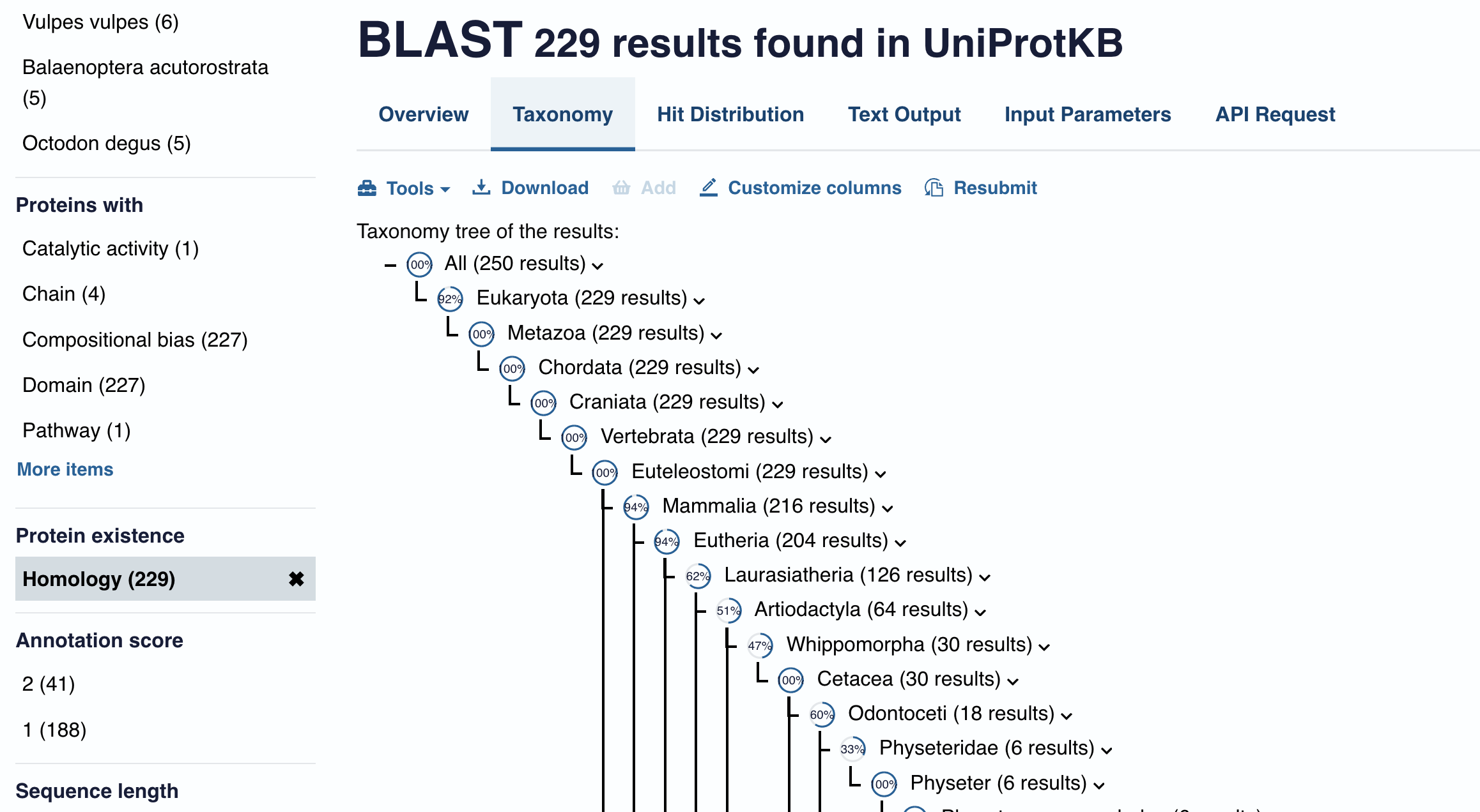
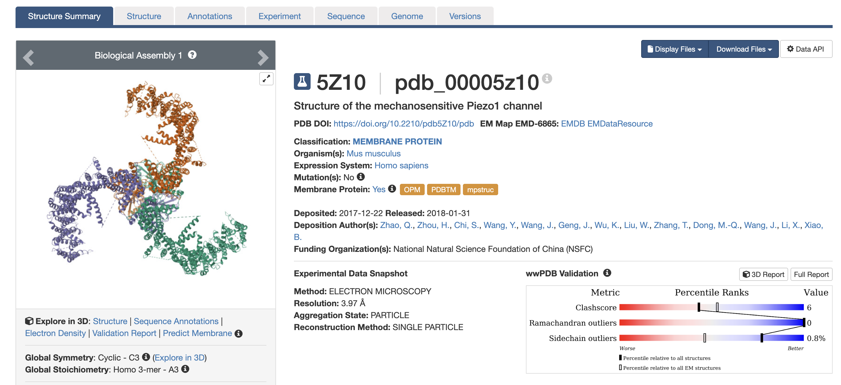
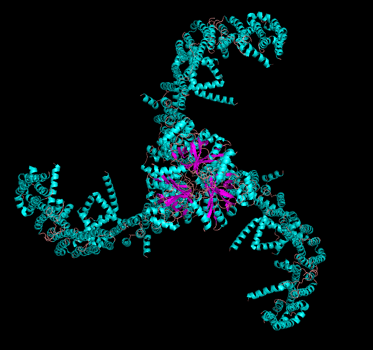
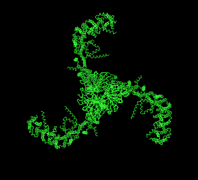
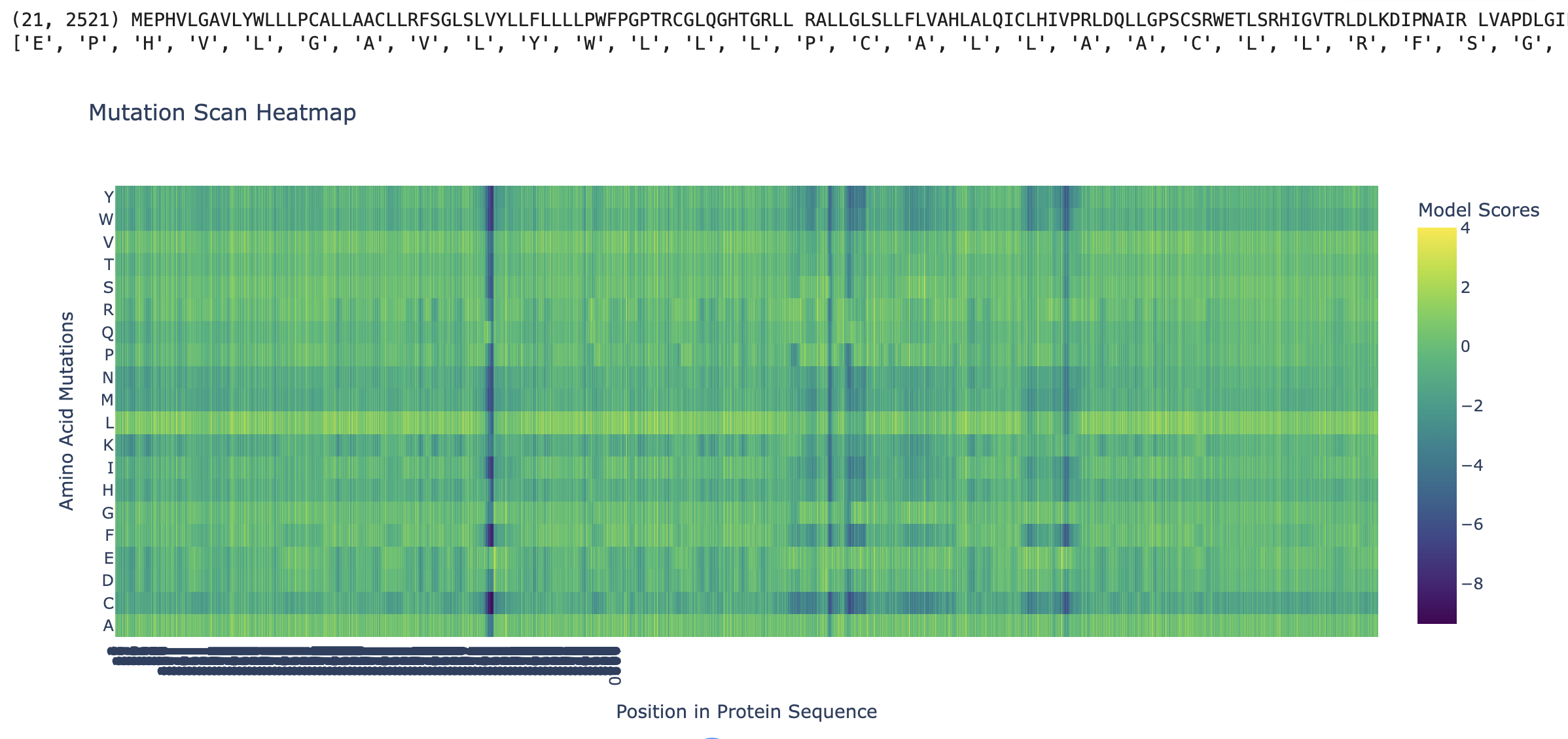
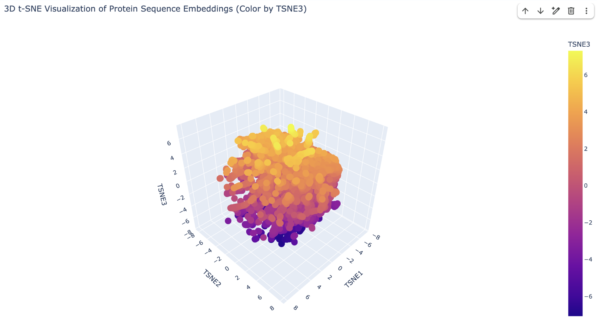
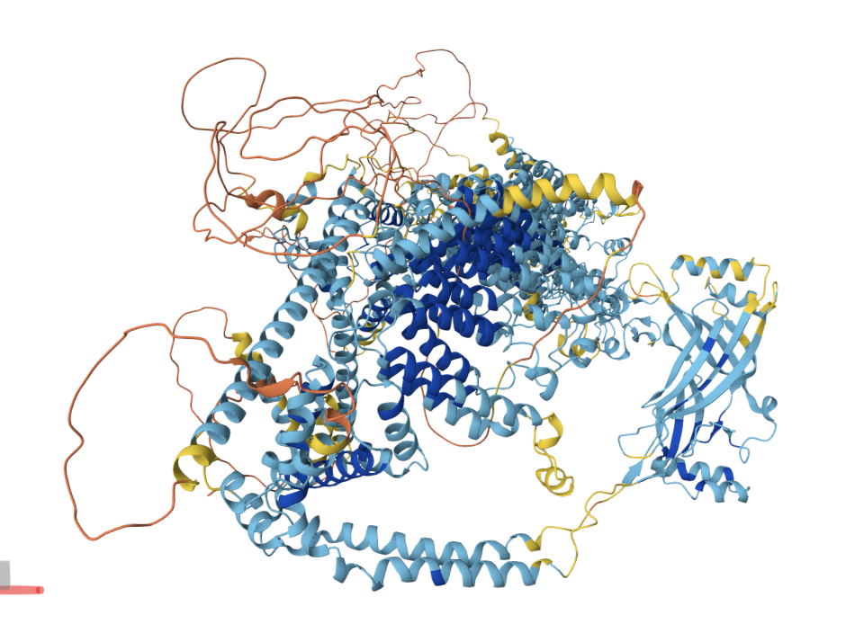


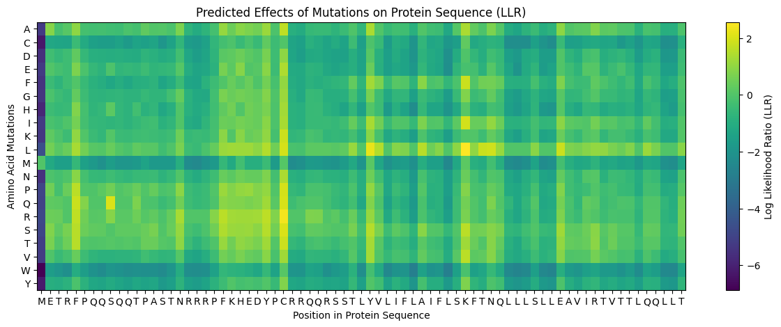


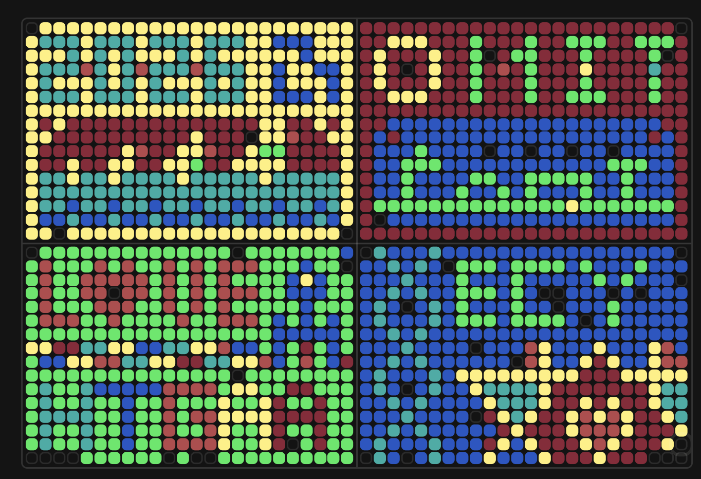

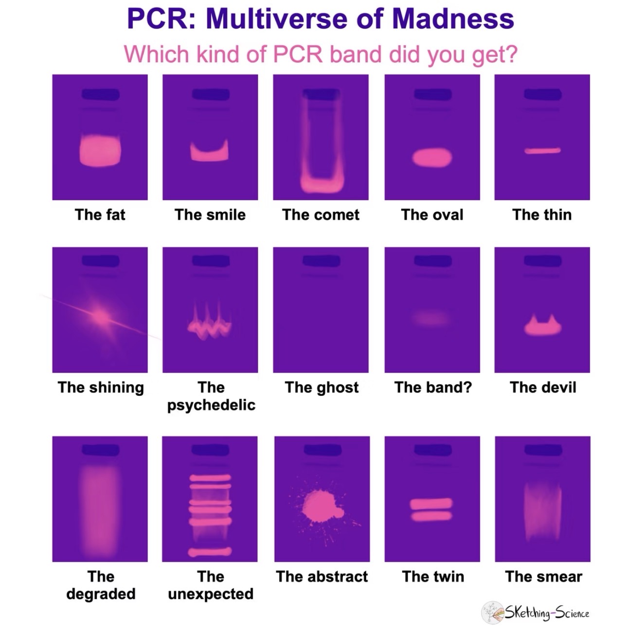


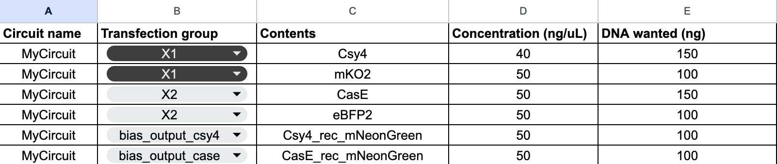
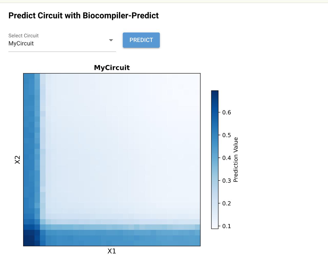
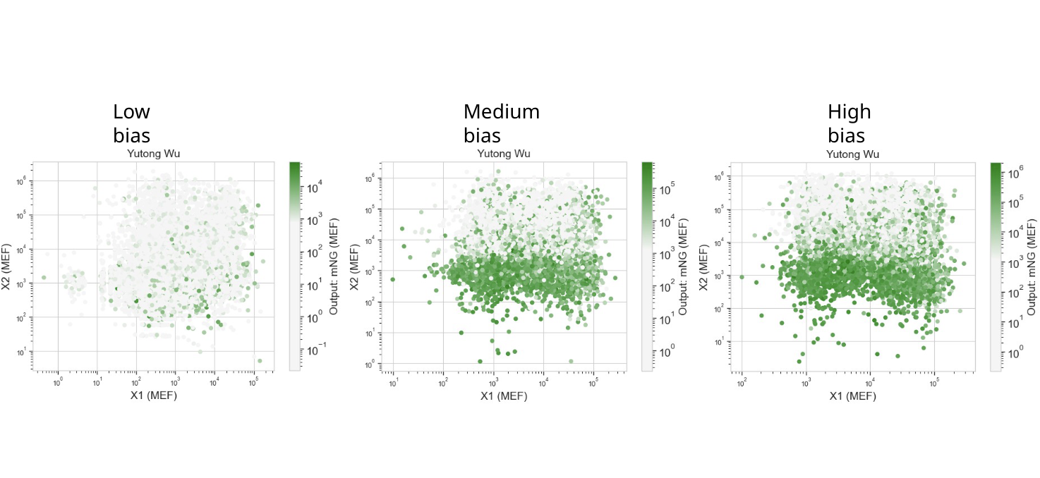


 The construct consists of two functional parts joined together: