Week 1 Lab: Pipetting

1. Objectives

By the end of this lab, you will be able to:

• Identify the three most common micropipette types and their volume ranges
• Correctly set and read a volume on a micropipette
• Demonstrate proper aspiration and dispensing technique
• Understand common pipetting errors and how to avoid them

2. Background — What Is a Micropipette?

A micropipette (commonly just called a “pipette” in the lab) is a precision instrument used to measure and transfer very small volumes of liquid — typically between 0.1 µL and 1000 µL (1 mL). Accurate pipetting is one of the most fundamental skills in biology, chemistry, and biomedical research. Even small errors in volume measurement can ruin an experiment, skew results, or waste expensive reagents.

Volumes in the lab are measured in:

💡 Quick reference: 1 mL = 1,000 µL. A typical raindrop is ~50 µL. A grain of salt is ~60 nL.

3. Pipette Types and Volume Ranges

There are three standard micropipettes you will use in this course. Each is color-coded and designed for a specific volume range. Never exceed the maximum or go below the minimum volume — this damages the internal piston mechanism.

⚠️ Rule: Always choose the pipette whose range most closely fits your target volume. Using a P1000 to measure 5 µL will be wildly inaccurate.

4. Parts of a Micropipette

         ┌────────────────┐
         │   Thumb Knob   │  ← Push down to aspirate / dispense
         │   (Plunger)    │
         └───────┬────────┘
                 │
         ┌───────┴────────┐
         │  Volume        │  ← Twist to set volume (DO NOT exceed range)
         │  Adjustment    │
         │  Dial          │
         └───────┬────────┘
                 │
         ┌───────┴────────┐
         │  Volume        │  ← 3-digit display window
         │  Display       │     (read top to bottom)
         │  Window        │
         └───────┬────────┘
                 │
         ┌───────┴────────┐
         │   Barrel /     │
         │   Body         │
         └───────┬────────┘
                 │
         ┌───────┴────────┐
         │  Tip Ejector   │  ← Press to eject used tip (never touch used tips)
         │  Button        │
         └───────┬────────┘
                 │
         ┌───────┴────────┐
         │  Tip Cone /    │  ← Where disposable tip attaches
         │  Shaft         │
         └───────┬────────┘
                 │
            [  Tip  ]        ← Disposable plastic tip (changes every use!)

5. Reading the Volume Display

The volume display has three digits read from top to bottom. How you interpret those digits depends on which pipette you are using.

P20 (range: 0.5 – 20 µL)

  ┌───┐
  │ 1 │   ← tens digit (µL)
  │ 5 │   ← ones digit (µL)
  │ 0 │   ← tenths digit (µL)
  └───┘
  = 15.0 µL

P200 (range: 20 – 200 µL)

  ┌───┐
  │ 1 │   ← hundreds digit (µL)
  │ 5 │   ← tens digit (µL)
  │ 0 │   ← ones digit (µL)
  └───┘
  = 150 µL

P1000 (range: 200 – 1000 µL)

  ┌───┐
  │ 1 │   ← thousands digit (µL)  
  │ 0 │   ← hundreds digit (µL)
  │ 0 │   ← tens digit (µL)
  └───┘
  = 1000 µL = 1.0 mL

6. Step-by-Step Pipetting Procedure

Step 1 — Set the Volume

Turn the volume adjustment dial to your desired volume.

• Turn clockwise to decrease volume
• Turn counter-clockwise to increase volume
• Never twist past the maximum — you will damage the piston

Step 2 — Attach a Tip

Press the tip cone firmly into a fresh pipette tip in the tip box. Give it a slight twist or firm push to create an airtight seal. Never touch the tip with your fingers after attachment — this contaminates your sample.

Step 3 — Pre-Wet the Tip (for accuracy)

Before aspirating your actual sample, aspirate and expel the liquid 2–3 times to wet the inner walls of the tip. This reduces evaporation error, especially important for small volumes (<10 µL).

Step 4 — Aspirate (Draw Up Liquid)

1. Hold the pipette vertically (or no more than 20° from vertical)
2. Press the plunger down to the first stop (you will feel resistance — do NOT push to the second stop yet)
3. Submerge the tip 2–3 mm into the liquid (P20/P200) or 3–6 mm (P1000)
4. Slowly and smoothly release the plunger — liquid will draw up into the tip
5. Wait 1–2 seconds, then withdraw the tip from the liquid by sliding it along the container wall

⚠️ Releasing too fast creates bubbles and inaccurate volumes. Speed matters!

Step 5 — Check for Bubbles

Hold the tip up to the light. If you see a bubble, expel the liquid and re-aspirate. Bubbles displace liquid and reduce your actual volume.

Step 6 — Dispense Liquid

1. Touch the tip to the inner wall of the destination tube or well at a slight angle
2. Press the plunger slowly to the first stop — this expels the set volume
3. Then press to the second stop (blow-out position) — this expels any remaining droplet
4. Keep the plunger depressed while withdrawing the tip from the container
5. Release the plunger slowly after the tip has cleared the liquid

Step 7 — Eject the Tip

Press the tip ejector button firmly over a waste container. Never remove used tips by hand — tips may be contaminated with biological or chemical material.

7. Common Pipetting Mistakes & How to Avoid Them

8. Accuracy vs. Precision

These two terms are distinct and both matter in pipetting:

• Accuracy — how close your measured volume is to the true intended volume
• Precision — how reproducible your measurements are across repeated trials

        Accurate &        Precise but         Neither
        Precise           Not Accurate        (Random)
        
          [X]              [ ][ ]              [ X ]
          [X]              [ ][ ]X           X [   ]
          [X]              [ ][ ]            [  X  ]
        ← target →       ← target →        ← target →

A pipette can be precise but inaccurate if it is mis-calibrated. Always check calibration before critical experiments.

9. Gravimetric Accuracy Test (Optional Practice Exercise)

You can test your pipetting accuracy by weighing water. Since water has a density of 1.00 g/mL, 100 µL of water should weigh exactly 0.100 g.

Protocol:

1. Tare (zero) an analytical balance with a microcentrifuge tube
2. Using a P200, set to 100 µL
3. Aspirate distilled water and dispense into the tube
4. Record the mass
5. Repeat 5 times and calculate the mean and % error

Data Table:

% Error formula:

% Error = |Measured − Expected| / Expected × 100

✅ Good pipetting: % error < 2% for P200 at 100 µL
⚠️ Acceptable: % error 2–5%
❌ Needs improvement: % error > 5%

10. Safety and Disposal

• Always use a new tip for each new liquid or sample
• Never pipette corrosive acids, bases, or organic solvents with a standard micropipette — use a repeat pipettor or serological pipette
• Dispose of used tips in the biohazard waste bin if biological material was handled, or regular waste otherwise
• If liquid enters the barrel of the pipette, stop immediately and notify your instructor — the piston must be cleaned and re-calibrated

Week 2 Lab: DNA Gel Art

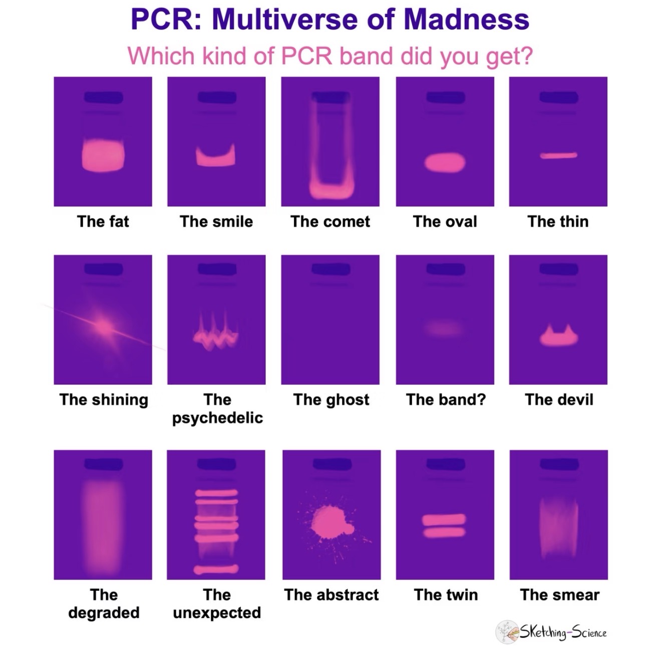
Image 1 (Mid-run photograph): The photograph taken during electrophoresis shows the gel submerged in TAE within the gel box. Two colored dye fronts are faintly visible — a blue band and a dark purple band — but they appear localized to only one or two lanes. The majority of the gel appears empty, with no visible dye migration in the other wells. This is already an early indicator that most wells were either not loaded successfully or contained insufficient DNA.

Image 2 (GeneSnap image): The final imaging result is largely dark. Only a single lane shows any detectable fluorescence — a faint, somewhat smeared signal concentrated in what appears to be one lane, with no clearly resolved discrete bands. The remaining lanes are entirely blank. This represents an unsuccessful gel run in terms of the intended gel art pattern.

Analysis of What Went Wrong Based on the observations made during lab sessions and the photographic evidence, several compounding factors likely contributed to the result:

1. Pipetting error during well loading. When I was loading the fourth slot, the pipette tip was not properly inserted into the well. This is a critical failure point. In submerged gel electrophoresis, the wells are filled with buffer. The loading dye’s density causes the sample to sink — but only if it is dispensed directly into the well. If the tip hovers above the well or is positioned outside it, the sample disperses into the surrounding buffer and is effectively lost. This likely explains why most lanes are empty on the final image.
2. Insufficient electrophoresis run time due to electrical issues. There was an unforeseen electrical short circuit that cut the run time short. This is consistent with the imaging result — even in the one lane that has signal, the DNA has not migrated very far, and there is no clear band resolution. A truncated run means fragments have not separated sufficiently, resulting in a compressed, smeared appearance rather than discrete bands. The faint dye fronts visible in Image 1 also suggest limited migration distance.
3. Potential variability in reaction preparation. Another plausible explanation adding to the result could be the differences in mixing or component proportions across the PCR tubes. This is plausible as if the Lambda DNA stock was not thoroughly vortexed or flicked, concentration could vary between tubes. Similarly, enzyme or buffer pipetting errors at the 1–3 μL scale are common and can result in incomplete digestion or no digestion at all, though the imaging suggests the bigger problem was DNA not being present in the wells at all.
4. Low overall signal intensity. Even the one visible lane is quite faint. This could indicate that the total DNA mass loaded was below the detection threshold of SYBR Safe under blue light excitation. With 1.5 μg of Lambda DNA per reaction and SYBR Safe staining, bands should normally be clearly visible. The faintness suggests either DNA was lost during loading, the stain was not adequately mixed into the gel, or the transilluminator exposure settings were suboptimal.

Week 3 Lab: Opentrons Art

Post-Lab Questions — Laboratory Automation & Final Project

Relevant Figures

Figure 1 — Automated Workflow Schematic

┌─────────────────────────────────────────────────────────────────────┐
│                  OT-2 Automated CFPS Screening Pipeline             │
│                                                                     │
│  DNA Library        CFPS Master Mix       Inducer Gradients         │
│  (384 constructs)   (cell extract +       (0 → 1000 µM)            │
│       │             energy system)               │                  │
│       │                  │                       │                  │
│       └──────────────────┴───────────────────────┘                  │
│                          │                                          │
│                    ┌─────▼──────┐                                   │
│                    │  OT-2 OT-2 │  ← Robotic dispensing            │
│                    │  Dispenser │     1–5 µL per well               │
│                    └─────┬──────┘                                   │
│                          │                                          │
│                    ┌─────▼──────┐                                   │
│                    │ 384-well   │  ← Reaction: 30°C, 6 h           │
│                    │   plate    │                                   │
│                    └─────┬──────┘                                   │
│                          │                                          │
│                    ┌─────▼──────┐                                   │
│                    │   Plate    │  ← GFP fluorescence               │
│                    │   Reader   │     (ex: 485nm / em: 520nm)       │
│                    └─────┬──────┘                                   │
│                          │                                          │
│                    ┌─────▼──────┐                                   │
│                    │  Python    │  ← Data analysis, dose-response   │
│                    │  Analysis  │     curve fitting, hit ranking    │
│                    └────────────┘                                   │
└─────────────────────────────────────────────────────────────────────┘

This figure represents the end-to-end automated pipeline: from DNA library preparation through robotic CFPS assembly, incubation, fluorescence readout, and computational analysis.

Figure 2 — Representative Dose-Response Heat Map (Conceptual)

        Inducer Concentration →
        0.01  0.1   1    10   100  1000  µM
       ┌─────┬─────┬─────┬─────┬─────┬─────┐
  C1   │ ░░░ │ ░░░ │ ▒▒▒ │ ▓▓▓ │ ███ │ ███ │  ← Strong biosensor
  C2   │ ░░░ │ ░░░ │ ░░░ │ ▒▒▒ │ ▓▓▓ │ ███ │  ← Medium response
  C3   │ ▒▒▒ │ ▒▒▒ │ ▒▒▒ │ ▒▒▒ │ ▒▒▒ │ ▒▒▒ │  ← Leaky (reject)
  C4   │ ░░░ │ ░░░ │ ░░░ │ ░░░ │ ░░░ │ ░░░ │  ← Non-functional
  C5   │ ░░░ │ ░░░ │ ▒▒▒ │ ███ │ ███ │ ███ │  ← Best hit: steep ON
       └─────┴─────┴─────┴─────┴─────┴─────┘
  
  Legend: ░ = Low fluorescence  ▒ = Medium  ▓ = High  █ = Maximum
  Rows = biosensor construct variants (C1–C5)
  Columns = inducer concentration

Each row represents a unique biosensor construct variant; each column a different inducer concentration. Construct C5 shows the steepest dose-response (ideal switch-like behavior) with minimal background — identified as the top hit for downstream validation.

References: Hossain et al. (2020) ACS Synth. Biol.; Pardee et al. (2014) Cell; Opentrons Protocol API v2 Documentation.

Week 6 Lab: Gibson Assembly

Week 6 Lab: Gibson Assembly Lab

Overview

In this experiment we engineer color variants of the purple Acropora millepora chromoprotein (amilCP) by introducing targeted mutations at the chromophore (CP) site: cagTGTCAGtac. Substituting the TGTCAG hexamer with variant codons shifts the expressed color to orange, pink, magenta, or blue, as described by Liljeruhm et al. (2018).

Part 1 covers the preparation of two PCR fragments — a Backbone fragment and a Color insert fragment — which will be joined by Gibson Assembly and transformed into E. coli in Part 2.

Progress: PCR Setup → Thermal Cycling → DpnI Digest → Purification → Gel Electrophoresis ✓ → Gibson Assembly) → Transformation)

Part 1 — PCR Reaction Setup

Time estimate: ~1.5 hours total

Two parallel PCR reactions were prepared on ice using the mUAV plasmid as template. The Backbone reaction amplifies the vector (ori + CmR + promoter + RBS), while the Color reaction amplifies the chromophore region with a mutant forward primer that introduces the desired codon substitution at the CP site.

Reagent Tables

Backbone DNA Fragment (Primers: Backbone Fwd + Backbone Rev)

Color DNA Fragment (Primers: Color Fwd + Color Rev)

Thermocycler Programs

Backbone Fragment (BB_PCR) — run on Bio-Rad T100, 25 µL volume

Initial Denature:   98°C · 30 sec
  ↻ 26 Cycles:
    Denature:       98°C · 10 sec
    Anneal:         57°C · 25 sec
    Extend:         72°C · 1.5 min
Final Extension:    72°C · 5 min
Hold:               12°C · ∞

Color Insert Fragment

Initial Denature:   98°C · 15 sec
  ↻ 26 Cycles:
    Denature:       98°C · 10 sec
    Anneal:         53°C · 20 sec
    Extend:         72°C · 15 sec
Final Extension:    72°C · 5 min
Hold:               12°C · ∞

The Color forward primer carries an intentional mismatch in the 6-bp chromophore region (e.g. TGTCAG → GTTGGA for orange). Because the mismatch sits in the 5′ overhang, Phusion polymerase still extends efficiently from the matched 3′ binding region. The mutation is thus incorporated into every PCR copy and all downstream clones.

Part 1a — DpnI Digest

⏱ Time estimate: 45 min at 37°C

After PCR, 1 µL of DpnI was added directly to each 25 µL reaction and incubated at 37°C for 30–60 minutes. DpnI recognises methylated 5′-G^m6ATC-3′ sequences present on E. coli-propagated plasmid template, but absent from unmethylated PCR products. The enzyme therefore selectively digests the parental template while leaving new amplicons intact.

Residual un-digested template will generate wildtype (purple) background colonies that compete with and obscure your color-mutant transformants.

Part 1b — DNA Purification & Quantification

⏱ Time estimate: 30 min

PCR products were purified using the Zymo DNA Clean & Concentrator kit (silica-column adsorption) to remove primers, dNTPs, polymerase, and buffer salts before Gibson Assembly.

Equipment & Consumables

• Zymo DNA Clean & Concentrator kit (columns + buffers)
• Eppendorf Centrifuge 5415C (set to 13,000 rpm, ≈ 17,900 × g)
• 1.5 mL microcentrifuge tubes
• 50 mL Falcon tube (liquid waste)
• Nanodrop or Qubit spectrophotometer
• P20 and P200 pipettes with tips
• Nuclease-free water

Procedure

1. Add 50 µL PCR product + 250 µL DNA Binding Buffer to a 1.5 mL tube. Vortex briefly.
2. Transfer all 300 µL to a Zymo-Spin Column seated in a Collection Tube. Centrifuge 1 min at 13,000 rpm. Discard flow-through; keep the collection tube.
3. Add 200 µL Wash Buffer. Centrifuge 1 min. Discard flow-through. Repeat once (2 washes total). Transfer column to a fresh 1.5 mL tube; discard the collection tube.
4. Add 6 µL nuclease-free water directly to the column membrane. Rest at room temperature for 2 min. Centrifuge 1 min. Collect and save the elution.
5. Measure concentration on Nanodrop: 2 µL per read. Target ≥ 30 ng/µL, A260/A280 ≈ 1.8–2.0.

Part 1c — Diagnostic Gel Electrophoresis

⏱ Time estimate: ~15 min at 100 V

Purified fragments were run on a 1% agarose E-Gel EX (Invitrogen) to confirm fragment sizes. Each lane received 3 µL sample + 3.3 µL 6× Loading Dye. DNA ladder loaded in lane M (leftmost).

Band Interpretation

Expected fragment sizes:

• Backbone: ~2800 bp (ori + CmR + promoter + RBS)
• Color insert: ~700 bp (24 bp upstream of CP site + chromophore + terminator)

Lanes 3 and 5 show bright, clean bands at the expected sizes for Color insert and Backbone respectively. Faint bands in lanes 1, 2, and 4 represent minor non-specific products that will be diluted out during Gibson Assembly and will not affect the outcome. Both fragments are confirmed — proceed to Gibson Assembly.

Part 2 — Transformation Results & Analysis

⏱ Incubation: 72 hours at 37°C | Selection: LB-Agar + Chloramphenicol 25 µg/mL

Colony Plates

Observation

All colonies across every plate — regardless of intended color variant (blue, pink, light pink) — express a uniform blue-purple color consistent with wildtype amilCP. The intended color shifts to pink or blue did not appear. One notable exception is the red-circled colony in the final plate (Fig. 5h), which is transparent/colorless.

Analysis

Imbalanced Insert:Backbone Molar Ratio

Gibson Assembly outcome is highly sensitive to the molar ratio of insert to backbone, not just the volumes used. The protocol specifies 0.5 µL backbone and 1.0 µL insert — but those volumes assume both fragments are at exactly the stated concentrations after purification.

When backbone is in excess, the probability of the two backbone ends annealing to each other increases sharply — rather than each end finding the insert:

Too much backbone → backbone ends self-anneal → re-circularization
                 → carries CmR + original amilCP promoter
                 → colonies survive selection AND express wildtype purple

Because the ratio imbalance originates in the Gibson reaction before transformation, it would affect all three volume groups (2µL, 4µL, 7µL) equally — explaining the consistency of the wildtype purple outcome across all plates.

transparent Colony

Partially succeeded, as this is consistent with a scenario where the backbone reassembled without the color insert — the Gibson exonuclease chewed back both ends of the backbone, they annealed to each other rather than to the insert, and ligase sealed the nick. The result is a backbone-only plasmid that carries CmR but lacks the amilCP CDS entirely, hence no color.

Alternatively, the insert was incorporated but with a frameshift or premature stop codon introduced during the Gibson join, knocking out chromoprotein expression without replacing it with a new color.

Either way, this colony is evidence that the Gibson Assembly chemistry was active and processing DNA correctly. The colorless result is not a failure — it is a partial success where the backbone was modified but the color swap did not complete as intended.

the wildtype blue-purple across all other colonies most likely reflects surviving template from incomplete DpnI digestion, while the single transparent colony shows that at least one genuine assembly event occurred.

Week 7 Lab: NeuroMorphic Circuits

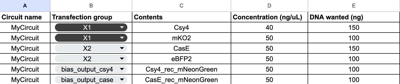
For the neuromorphic circuit, our group aimed to design a “L” shaped heatmap. We added two bias corresponding to X1 and X2 ERNs.

Looked perfect

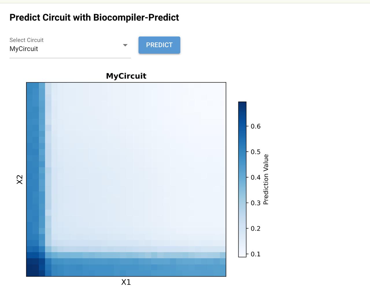
I think we might’ve submitted the wrong file ahahaha, so the final output only displayed the bottom part of the “L”

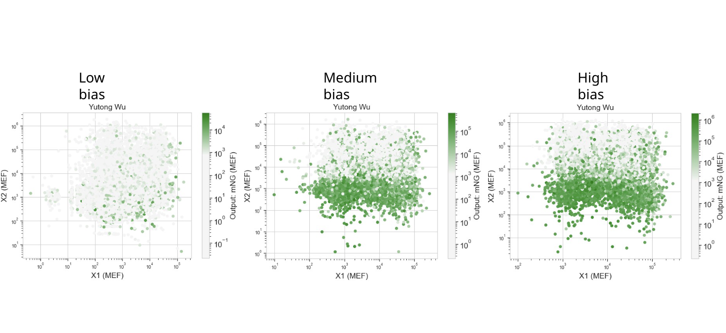
Each dot in these scatterplots represents a single human cell. The color shows the level of output (mNeonGreen) as a function of X1 and X2 and, optionally, varying levels of bias.

Week 11 Lab: Cloud Labs

1. Given the 6 fluorescent proteins we used for our collaborative painting, identify and explain at least one biophysical or functional property of each protein that affects expression or readout in cell-free systems (hint: options include maturation time, acid sensitivity, folding, oxygen dependence, etc) (1-2 sentences each).

The amino acid sequences are shown in the HTGAA Cell-Free Benchling folder.

sfGFP: primary advantage is robust folding kinetics; it is engineered to fold correctly even when fused to insoluble proteins, making it highly resistant to aggregation in the crowded environment of a cell-free extract.

mRFP1: characterized by slow maturation kinetics and a tendency for photobleaching; the delay between peptide synthesis and chromophore formation can lead to an underestimation of protein yield in short-term reactions.

mKO2: features fast maturation and oxygen dependence; while it reaches peak fluorescence quickly, the final oxidative step of chromophore formation requires sufficient O2 levels, which may become limiting in deep-well plates.

mTurquoise2: known for high quantum yield and acid stability; its low pKa makes it less sensitive to the $pH$ drops that naturally occur as metabolic byproducts (like organic acids) accumulate during long-term cell-free incubation.

mScarlet_I: a high-brightness variant with accelerated maturation compared to earlier red FPs; however, it remains sensitive to the oxidative environment, as oxygen is required to complete the cyclization of its chromophore.

Electra2: optimized for ultra-fast maturation; its rapid “time-to-bright” makes it the ideal candidate for real-time monitoring of transcription-translation (TX-TL) kinetics where immediate feedback is required.

2. Create a hypothesis for how adjusting one or more reagents in the cell-free mastermix could improve a specific biophysical or functional property you identified above, in order to maximize fluorescence over a 36-hour incubation. Clearly state the protein, the reagent(s), and the expected effect.

Protein: mScarlet_I

Reagent Adjustment: Increase Glucose and Nicotinamide concentrations while utilizing a semi-permeable reaction seal.

Expected Effect:In a 36-hour run, the primary bottleneck for a bright red FP like mScarlet_I is the depletion of energy and the requirement for oxygen for chromophore maturation. By increasing Glucose and Nicotinamide, we extend the metabolic “runway” for $ATP$ regeneration via the NMP-Ribose-Glucose pathway; combining this with a semi-permeable seal ensures a constant influx of O2 to drive the oxidative maturation of the chromophore, thereby maximizing the total fluorescent signal over the extended incubation period.

The second phase of this lab will be to define the precise reagent concentrations for your cell-free experiment. You will be assigned artwork wells with specific fluorescent proteins and receive an email with instructions this week (by 4/24). Make sure that your final project slide is in the slide deck below to be included!

The final phase of this lab will be analyzing the fluorescence data we collect to determine whether we can draw any conclusions about favorable reagent compositions for our fluorescent proteins. This will be due a week after the data is returned (TBD!).