Subsections of Homework
Week 1: Principles and Practices
1. Describe a biological engineering application or tool you want to develop and why.
I was reading this review paper, “Engineering bacterial warriors: harnessing microbes to modulate animal physiology”[1]. There’s a section that talks about engineering bacteria that can help corals survive heat stress, like making bacteria that clean up harmful reactive oxygen species (ROS) when water gets too warm [Figure 1]. The paper also discusses transplanting entire communities of beneficial microbes from resilient corals to vulnerable ones (Coral Microbiome Transfer, or CMT) [1,2]. The whole concept of using Beneficial Microorganisms for Corals (BMC) is really promising [3].
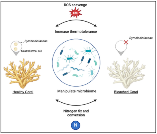 Figure 1. Engineered microbes have the capacity to assist corals in alleviating environmental stresses [1].
However, the authors point out major deployment challenges [1, 4]. The effects of introducing new bacteria are unpredictable, and they could outcompete or disrupt the coral’s natural microbiome. Currents could also scatter free bacteria before they even reach the target corals. At the moment, there’s no way to control the dosage or how long the coral is exposed, making the treatment inefficient and potentially wasteful. In essence, it’s difficult to introduce these engineered microbes effectively in the ocean.
The next section of the paper was about human health, discussing how engineered bacteria are being developed for targeted disease therapy [1]. This got me thinking about medical delivery systems, things like timed-release pills, biodegradable implants, or hydrogels that release drugs right where they’re needed in the body. The principle for all these applications is the same, to protect the therapeutic agent and control its release at the target site. So I thought something similar could be done for coral reefs.
I looked into existing coral probiotic delivery systems and came across a smart underwater microbial delivery system for coral reef habitat recovery developed by researchers at KAUST [5]. This system uses a buoy, an FPGA computer, cameras, and AI to monitor coral color and automatically pump probiotics into the water [Figure 2]. However, its complexity, cost, and reliance on pumping microbes into the water column still face some of the core challenges mentioned in the review paper, like dosage control and localization.
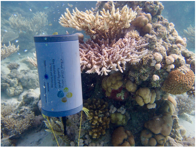 Figure 2. Smart underwater microbial delivery system for coral reef habitat (KAUST) [5].
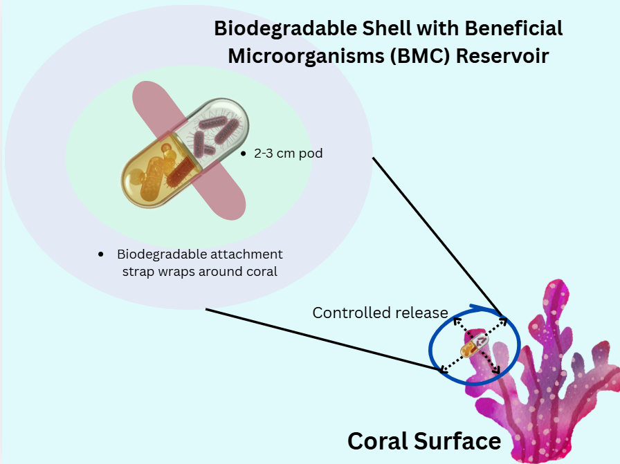
To address the limitations of bulk water delivery, I propose a more targeted approach: a small, biodegradable pod, like a micro-infusion pump specifically for a coral. The pod would be able to attach directly to the coral’s surface to create a localized environment where the release of beneficial bacteria can be controlled. This would allow for a slow and sustained colonization of the coral’s microbiome, making the delivery more efficient and less wasteful than other methods. Diver or robotic systems would be able to precisely deploy the pods which allows for targeted intervention on corals identified as the most at-risk or ecologically valuable for reef recovery.
This idea of targeted, contained delivery isn’t completely new. In agriculture, technologies like coated seeds or biodegradable granules are standard for protecting and delivering beneficial microbes to plant roots [6]. For corals, scientists are already exploring direct methods like “Bacterioplankton” or gels [4]. A small, attachable pod builds on these principles and turns a massive ecological problem into a tangible engineering challenge to deliver a single, effective device.
Sketch of the idea:
References
Gao B, Ruiz D, Case H, Jinkerson RE, Sun Q. Engineering bacterial warriors: harnessing microbes to modulate animal physiology. Curr Opin Biotechnol. 2024;87:103113. doi:10.1016/j.copbio.2024.103113.
Doering T, Wall M, Putchim L, Rattanawongwan T, Schroeder R, Hentschel U, et al. Towards enhancing coral heat tolerance: a “microbiome transplantation” treatment using inoculations of homogenized coral tissues. Microbiome. 2021;9(1):102. doi:10.1186/s40168-021-01053-6.
Peixoto RS, Rosado PM, Leite DCA, Rosado AS, Bourne DG. Beneficial microorganisms for corals (BMC): proposed mechanisms for coral health and resilience. Front Microbiol. 2017;8:341. doi:10.3389/fmicb.2017.00341.
Damjanovic K, van Oppen MJH, Menéndez P, Blackall LL. The contribution of microbial biotechnology to mitigating coral reef degradation. Microb Biotechnol. 2017 Jul 11;10(5):1236–1243. doi: 10.1111/1751-7915.12769.
Filho J. A smart underwater microbial delivery system for coral reef habitat recovery. InnovateFPGA. 2022 (cited 2026 February 8). Available from: https://www.innovatefpga.com/cgi-bin/innovate/teams.pl?Id=EM043.
Bashan Y, de-Bashan LE, Prabhu SR, Hernandez JP. Advances in plant growth-promoting bacterial inoculant technology: formulations and practical perspectives (1998-2013). Plant Soil. 2014;378(1):1-33. doi:10.1007/s11104-013-1956-x.
2. Describe one or more governance/policy goals related to ensuring that this application or tool contributes to an “ethical” future, like ensuring non-malfeasance (preventing harm). Break big goals down into two or more specific sub-goals.
To ensure the ethical development and deployment of the coral probiotic pod, I propose adapting the governance framework outlined in the Synthetic Genomics: Options for Governance report [7]. The framework focuses on Safety, Security, Responsibility, and Oversight which together provide a clear structure to address the environmental and social challenges of engineering interventions in sensitive ocean ecosystems.
Goal 1: Safety – Establishing a Risk Assessment Protocol
Preventing unintended harm to reef ecosystems requires a phased approach that mirrors established biocontainment principles. This begins with pre-deployment screening in which any engineered microbial strain undergoes standardized laboratory assessment to confirm:
- Non-pathogenic to a panel of key reef organisms (corals, fish, crustaceans)
- Non-toxic in terms of metabolites produced
- Assessed for its competitive impact on the native coral microbiome
Following lab validation, a mandatory phased testing pathway should be implemented. Initial trials would occur in a controlled aquarium system simulating reef conditions. Successful results could then progress to caged in-situ trials, where pods are deployed within permeable enclosures on actual reefs to monitor ecological interactions under natural but contained conditions.
Goal 2: Security – Implementing a Function-Limited Use Framework
To address dual-use concerns inherent to programmable delivery systems, governance should focus on restricting applications to predefined beneficial functions. One approach involves establishing a “Positive List” of approved microbial functions, such as ROS-scavenging or nutrient provision, for coral restoration. An organization like the European Marine Research Network (EuroMarine) could maintain this public, evidence-based registry. Delivery of any agent performing functions not on this list would be prohibited. Complementing this, procedural security measures would include certification training for users in secure handling and deployment protocols, and restricting access to advanced engineered strains to institutions operating under established biosafety and biosecurity frameworks.
Goal 3: Responsibility – Ensuring Equitable Access and Procedural Justice
To align development with principles of environmental justice and accessibility, the pod’s mechanical design should follow an open-source model. 3D printable files and assembly guides should be published under a non-commercial conservation license to democratize access and enable local adaptation. Additionally, formal stakeholder consultation processes should be integrated into deployment planning. Engaging coastal communities, fishery cooperatives, and tourism boards from the start of the project would ensure local ecological knowledge informs implementation and aligns with community-defined priorities.
Goal 4: Oversight – Creating an Adaptive Governance Structure
Effective implementation requires mechanisms for ongoing evaluation and adaptation. A multidisciplinary advisory panel should comprise marine ecologists, synthetic biologists, social scientists, ethicists, and community representatives. They would provide oversight by reviewing field trial proposals and periodically updating the “Positive List” and testing protocols based on emerging research. This could be supplemented by a centralized deployment registry documenting key metadata (location, probiotic function, scale, responsible entity) to enable accountability and long-term impact monitoring.
References
- Garfinkel MS, Endy D, Epstein GL, Friedman RM. Synthetic Genomics: Options for Governance. J. Craig Venter Institute; 2007. Available from: https://www.jcvi.org/research/synthetic-genomics-options-governance.
3. Describe at least three different potential governance “actions” by considering the four aspects below (Purpose, Design, Assumptions, Risks of Failure & “Success”)
Action 1: Establishing a Mandatory ‘Reef-Safe’ Biopolymer Certification
- Purpose: Current material standards, such as the EU’s compostability criteria or general marine biodegradation tests, are not designed for devices in direct, sustained contact with sensitive coral reef ecosystems [8]. A new certification is needed to prevent pollution or toxic leaching from pod materials.
- Design: The European Committee for Standardization (CEN) could develop this certification in consultation with groups like the International Coral Reef Initiative (ICRI). It would build on existing marine biodegradation tests (like ISO 18830) but add specific ecotoxicity assays [9,10]. In the UK, Defra could require this certification for Marine Management Organisation (MMO) deployment permits [11].
- Assumptions: This assumes lab tests accurately predict real-world impacts and that certification won’t be too burdensome for conservation projects.
- Risks of Failure & “Success”: The action could fail if perceived as bureaucratic overreach, leading to low adoption or non-compliance. A significant risk of success is ‘greenwashing,’ where achieving material certification creates a false sense of security and diverts attention from necessary ecological monitoring of the probiotic function itself.
Action 2: Creating an Open-Source Hardware Repository Hosted by a Research Consortium
- Purpose: Open-source approaches have worked well in conservation technology. Applying this model to the pod system would prevent proprietary lock-in and encourage adaptation, aligning with funder open-access policies [12,13].
- Design: A consortium like EuroMarine could host the repository. Designs would use licenses like CERN Open Hardware, with governance similar to successful citizen science platforms, allowing vetted contributions while maintaining quality control.
- Assumptions: Without an active community, the repository could stagnate. Success might paradoxically lead to commercial co-option, where companies create proprietary versions that limit equitable access.
- Risks of Failure & “Success”: Failure could stem from repository stagnation without dedicated curation. Additionally, success could lead a for-profit entity to create a proprietary, locked version of the core open design, potentially undermining the goal of equitable access.
Action 3: Implementing Mandatory Pre-Deployment Registration in Existing Public Registers
- Purpose: While transparency is required by EU and UK marine laws, no registry exists for coral interventions. This action would fill that gap by extending existing systems.
- Design: In the UK, the MMO could add a coral intervention module to its Marine Case Management System [11]. For international waters, the UN’s Biosafety Clearing-House (BCH) already tracks living modified organisms and could serve as a model [14]. Funders could require registration as a grant condition.
- Assumptions: This assumes existing systems can be adapted affordably and that transparency itself encourages responsible behavior.
- Risks of Failure & “Success”: Cumbersome processes might reduce compliance. If successful, registry clutter could obscure important projects, and public listings might attract opposition to legitimate research.
References
- Wei L, McDonald AG, Stark NM. Biodegradable polymers in the marine environment: current status and future perspectives. Environ Sci Technol. 2021;55(9):4203-17.
- International Organization for Standardization. Plastics — determination of aerobic biodegradation of non-floating plastic materials in a seawater/sandy sediment interface — method by measuring the oxygen demand in closed respirometer. ISO 18830:2018.
- European Committee for Standardization. Who we are (Internet). Brussels: CEN; 2023 (cited 2026 Feb 8). Available from: https://www.cen.eu.
- Department for Environment, Food & Rural Affairs. Marine and Coastal Access Act 2009: guidance (Internet). (cited 2026 Feb 8). Available from: https://www.legislation.gov.uk/ukpga/2009/23/contents.
- European Commission. Horizon Europe programme guide (Internet). Brussels: European Commission; 2021 (cited 2026 Feb 8). Available from: https://ec.europa.eu/info/funding-tenders/opportunities/docs/2021-2027/horizon/guidance/programme-guide_horizon_en.pdf.
- UK Research and Innovation. UKRI open access policy (Internet). Swindon: UKRI; 2022 (cited 2026 Feb 8). Available from: https://www.ukri.org/publications/ukri-open-access-policy/.
- Secretariat of the Convention on Biological Diversity. The Biosafety Clearing-House (BCH) (Internet). Montreal: SCBD; 2023 (cited 2026 Feb 8). Available from: https://bch.cbd.int/.
4. Score (from 1-3 with, 1 as the best, or n/a) each of your governance actions against your rubric of policy goals. The following is one framework but feel free to make your own:
| Does the option: | Option 1 | Option 2 | Option 3 |
|---|---|---|---|
| Enhance Biosecurity | |||
| • By preventing incidents | 1 | 3 | 2 |
| • By helping respond | 2 | 1 | 1 |
| Foster Lab Safety | |||
| • By preventing incident | 2 | n/a | n/a |
| • By helping respond | 2 | n/a | n/a |
| Protect the environment | |||
| • By preventing incidents | 1 | 2 | 2 |
| • By helping respond | 3 | 3 | 1 |
| Other considerations | |||
| • Minimizing costs and burdens to stakeholders | 3 | 1 | 1 |
| • Feasibility? | 2 | 1 | 1 |
| • Not impede research | 2 | 1 | 1 |
| • Promote constructive applications | 1 | 1 | 1 |
5. Drawing upon this scoring, describe which governance option, or combination of options, you would prioritize, and why. Outline any trade-offs you considered as well as assumptions and uncertainties.
Based on the scoring, I would prioritize implementing Option 2 and Option 3 combined. Looking at the table, Option 2 and Option 3 both score a “1” on all of the “Other considerations” section. That means that they minimize burden, are highly feasible, don’t impede research, and promote good applications. This is important for a new tool meant to address an urgent problem like coral bleaching. If governance is too heavy-handed from the start, it could hinder the innovation and collaboration that’s needed. The trade-off is that Option 2, by itself, scores a “3” on preventing biosecurity incidents. Making designs freely available could, in theory, make misuse easier. This is where Option 3 creates counterbalance because it scores a “1” on helping respond to incidents across biosecurity and environmental protection. By pairing them, it would create a system with the tools to build the coral probiotic pod and help reefs, and it would create transparency and accountability by asking users to outline where, when, and what they’re doing with the tools.
Although Option 1 is undeniably important, it scores low on burden, feasibility and potential to impede research. Strict certification could potentially stall projects, which is why it’s important to begin by requiring the use of characterized and safe materials documented in the open-source repository (Option 2) and logged in the registry (Option 3). As the field matures and the most effective materials become clear, a formal certification like Option 1 can be developed based on real-world data, making it more practical and accepted.
This decision comes with the assumption that the primary users, such as researchers, and conservation NGOs, would be acting in good faith. The governance is primarily designed to support and guide a responsible community, not solely to thwart a malicious one. There’s also uncertainty regarding compliance with the registration system of Option 3. The system would only work if people actually use it, which depends heavily on enforcement tactics like making it a requirement for grant funding from UKRI or Horizon Europe, for example [12,13]. The main trade-off is accepting a potentially higher risk of a small-scale indicent by lowering barriers to entry with Option 2 in exchange for greater capacity for widespread, adaptive learning and rapid scaling. For a crisis like reef degradation, where rapid experimentation is needed, this seems like the necessary and ethical choice.
References
- European Commission. Horizon Europe programme guide (Internet). Brussels: European Commission; 2021 (cited 2026 Feb 8). Available from: https://ec.europa.eu/info/funding-tenders/opportunities/docs/2021-2027/horizon/guidance/programme-guide_horizon_en.pdf.
- UK Research and Innovation. UKRI open access policy (Internet). Swindon: UKRI; 2022 (cited 2026 Feb 8). Available from: https://www.ukri.org/publications/ukri-open-access-policy/.
Homework Questions from Professor Jacobson
- Nature’s machinery for copying DNA is called polymerase. What is the error rate of polymerase? How does this compare to the length of the human genome. How does biology deal with that discrepancy?
The error rate of DNA polymerase with its intrinsic proofreading function is approximately 1 error per 10⁶ bases incorporated (1:10⁶ or 10⁻⁶). the human genome has approximately 3.2 billion base pairs (3.2 x 10⁹ bp), that means there are about 3,200 errors per genome duplication. To deal with the discrepancy, there’s a third layer of correction called DNA Mismatch Repair (MMR). This is a post-replication system that acts after the polymerase has moved on. Specialized proteins scan newly synthesized DNA, identify mismatches that escaped proofreading, excise the erroneous segment, and resynthesize it correctly. In this way, MMR improves fidelity by an additional 100 to 1000-fold, so that the new error rate is about 1 error per 10⁹ to 10¹⁰ bases. Compared to the human genome, that’s about 0.3 errors per genome duplication.
- How many different ways are there to code (DNA nucleotide code) for an average human protein? In practice what are some of the reasons that all of these different codes don’t work to code for the protein of interest?
An average human protein has around 400 amino acids, and each of the 20 amino acids is encoded by 1-6 codons. Using average codon degeneracy (3 codons/amino acid), the possible sequences is around 3400, or roughly 10190 different DNA sequences. In practice all of these codes don’t work to code for the protein for several reasons. First, cells prefer certain codons for efficient translation because rare codons slow down protein production. Also, some sequences form stable structures that hinder ribosome binding or translation initiation, and these sequences could also create unintended splice sites that disrupt mRNA processing. Additionally, sequences like repeats or high GC content can cause recombination or mRNA degradation.
Homework Questions from Dr. LeProust
- What’s the most commonly used method for oligo synthesis currently?
The most commonly used method for oligo synthesis currently is the phophoramidite method developed by Caruthers in 1981.
- Why is it difficult to make oligos longer than 200nt via direct synthesis?
It’s difficult to make oligos longer than 200nt via direct synthesis because of the cumulative stepwise yield. Since the synthesis occurs in a cycle, so it compounds with each added based becoming inefficient and costly. After 200 cycles, even at 99.5% efficiency, only about 37% of the growing chains are the correct full-length product. The other shorter chains would be failed sequences that have to be removed.
- Why can’t you make a 2000bp gene via direct oligo synthesis?
The yield for a 2000nt strand would be very low which is impractical. Due to the high intrinsic error rate of chemial synthesis, in a 2000bp molecule there would be around 20 random errors which would make the gene non-functional.
Homework Question from George Church
[Using Google & Prof. Church’s slide #4] What are the 10 essential amino acids in all animals and how does this affect your view of the “Lysine Contingency”?
The 10 essentiall amino acids in all animals are: Cysteine (Cys), Histidine (His), Isoleucine (Ile), Leucine (Leu), Lysine (Lys), Methionine (Met), Phenylalanine (Phe), Threonine (Thr), Tryptophan (Trp), and Valine (Val) [1].
The “Lysine Contingency” is a fictional genetic modification from Jurassic Park that was designed to make engineered dinosaurs dependent on lysine supplements, causing them to die without them [2]. However, knowing the full list of essential amino acids significantly weakens the possibility of the contingency since lysine is not uniquely essential. It’s one of ten amino acids that animals cannot synthesize de novo. A predator deficient in any of these would most like have severe growth impairment, immune dysfunction, and eventually death. Additionally, animals get these essential amino acis from their diet. That means the contingency relies on the assumption that lysine is not available in the natural environment. However, lysine, like all the other essential amino acis, is abundant in protein-rich foods which a carnivorous dinosaur would depend on. Even herbivorous dinosaurs would acquire these amino acis through a varied plant diet. Therefore, the dinosaurs would probably meet their lysine requirement through their normal feeding behavior, which would make the contingency ineffective.
References
- Hou Y, Wu G. Nutritionally Essential Amino Acids. Advances in Nutrition (Internet). 2018 Sep 15;9(6):849–51. Available from: https://www.ncbi.nlm.nih.gov/pmc/articles/PMC6247364/.
- Lysine contingency (Internet). Jurassic Park Wiki. Available from: https://jurassicpark.fandom.com/wiki/Lysine_contingency.
Week 2: DNA Read, Write, & Edit
Part 1. Benchling & In-silico Gel Art
This week’s lab followed the protocol detailed in “Gel Art: Restriction Digests and Gel Electrophoresis”. The first step was to make a free account at benchling.com and import the Lambda DNA as seen in [Figure 1] below.
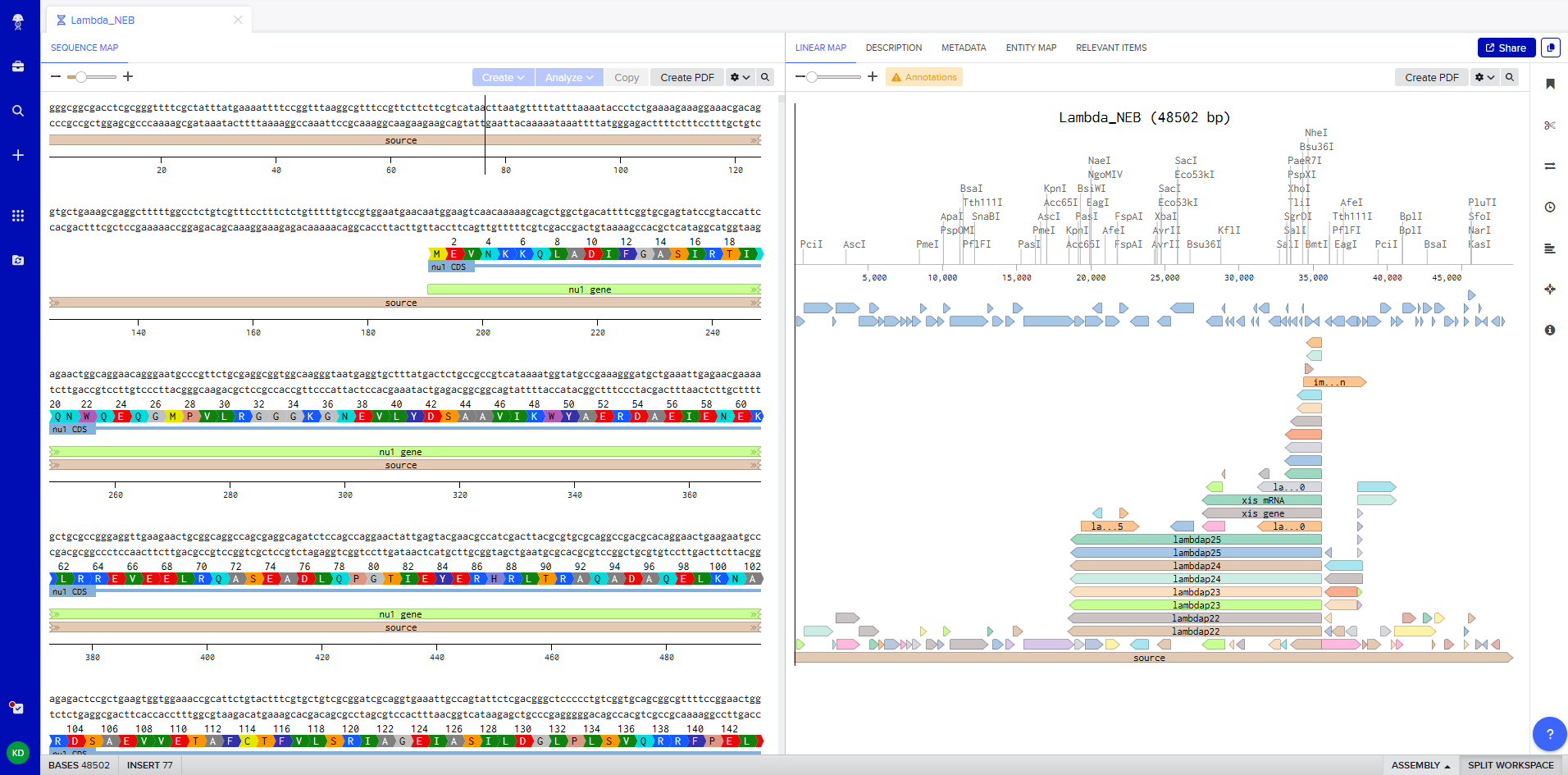 Figure 1. Imported the Lambda DNA.
The next step was to simulate restriction enzyme digestion with the following enzymes:
- EcoRI
- HindIII
- BamHI
- KpnI
- EcoRV
- SacI
- SalI
Figure 2 shows the virtual digest with EcoRI and Figure 3 shows the virtual digest with all the enzymes mentioned above.
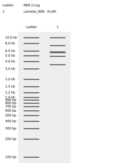 Figure 2. EcoRI virtual digest.
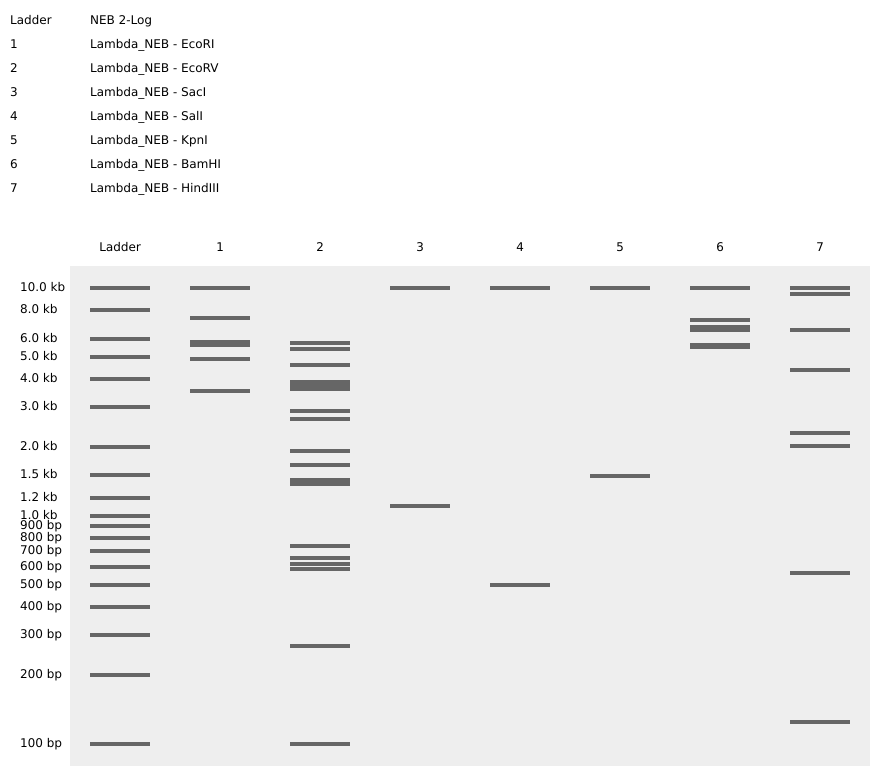 Figure 3. Full virtual digest.
The last step was to create a pattern/image in the style of Paul Vanouse’s Latent Figure Protocol artworks. For this I used Ronan’s website which was a helpful tool to iterate designs, especially since the physical lab experiment could not be carried out due to lab and equipment restrictions.
This was my original idea to make a penguin:
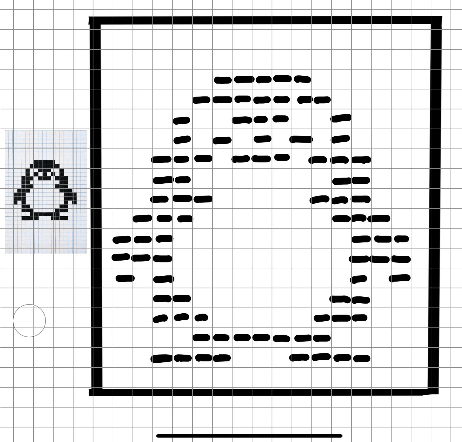 Figure 4. Pixel penguin sketch.
The result using Ronan’s website:
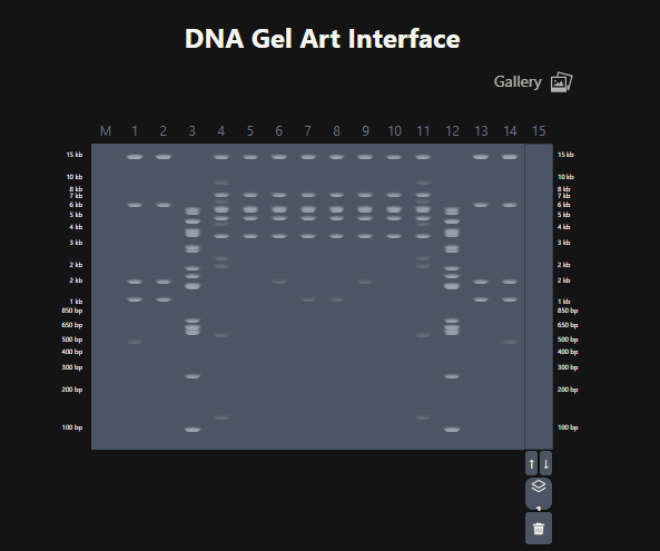 Figure 5. Attempt at designing a penguin in the style of latent Figure Protocol.
These are the gel restriction digest per row:
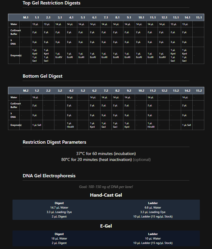 Figure 6. Tables of restriction enzymes used per row and per layer.
Part 3: DNA Design Challenge
1. Choose your protein.
For the Week 1 HW I focused on engineering a biodegradable pod that would control the release of localized beneficial bacteria that could help corals survive heat stress. For this week’s HW, I’ve selected the protein manganese superoxide dismutase (MnSOD) which is the enzyme that helps corals neutralize harmful reactive oxygen species (ROS). When ocean temperatures rise during bleaching events, corals experience oxidative stress, and their cells produce dangerous levels of superoxide radicals (O₂⁻). MnSOD is part of the coral’s natural antioxidant defense system, converting these damaging radicals into hydrogen peroxide (H₂O₂) and oxygen (O₂) [1], which are then further neutralized by other enzymes like catalase.
Protein Selected: Manganese Superoxide Dismutase (MnSOD) from Stylophora pistillata
Accession Numbers:
- UniProt: A3KLM5 (A3KLM5_STYPI)[2]
- NCBI GenBank: AAX99423.1[3]
Organism: Stylophora pistillata (Smooth cauliflower coral)
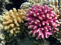 Figure 1. A photo of Stylophora pistillata [4].
Length: 156 amino acids (partial sequence)
Protein Existence: Evidence at transcript level
Protein Sequence:
AAX99423.1 manganese superoxide dismutase, partial [Stylophora pistillata] YDYDALQPAISAEIMQLHHQKHHATYVNNLNVAAEEKFSEAQAKGDTSAMISLQPALKFNGGGHINHSIFWTNLSPNGGGEPT GALMEAIKEDFGSFENFKERFNAATVAVQGSGWGWLGYSKADKGLVITTCANQDPLQATTGLVPLLGMDVWEHA
2. Reverse Translate: Protein (amino acid) sequence to DNA (nucleotide) sequence.
Using the Central Dogma framework, I worked backwards from the MnSOD protein sequence to find its corresponding DNA sequence. The protein sequence I selected (AAX99423.1) was originally derived from the mRNA record AY916505.1 [2,5]. Because this record includes a /codon_start=3 annotation, I removed the first two nucleotides (which likely represent 5’ UTR sequence) to obtain the actual coding sequence. The resulting 468-nucleotide sequence (156 codons) exactly matches the partial MnSOD protein.
DNA sequence (from NCBI AY916505.1):
MnSOD DNA sequence (partial cds) tacgatgctttacaaccagcaatcagtgcagaaattatgcaacttcatcaccagaaacatcatgcaacatatgtgaacaacttgaatgtagccgaagaaaagttttctgaggcgcaagctaaaggagataccagtgctatgatatcactccagccagccttgaaattcaatggaggaggacatattaatcactcaatattttggacaaatctctctcctaatggtggaggtgaaccaacaggagccttgatggaagctatcaaggaagactttggttcatttgaaaactttaaggaaaggttcaatgcagcaactgtagctgtgcagggctcaggatggggttggctgggttatagcaaggctgacaagggcctggtgatcaccacatgtgccaatcaagaccctctccaggccaccacaggactggtgccacttcttggaatggatgtctgggaacacgca
3. Codon optimization.
Codon optimization is necessary because of codon usage bias. Most amino acids are encoded by multiple codons, however, different organisms have evolved preferences for specific codons based on the availability of matching tRNA molecules in their cells [6,7]. For example, attempting to express the coral MnSOD gene in E. coli could result in low protein yield, truncated proteins, or no expression at all because there would be codons that are rare in bacteria [7]. By codon-optimizing the sequence, the coral gene is essentially translated for the host organism to replace those rare codons with preferred ones but still maintaining the same amino acid sequence. This maximizes translational efficiency and protein yield.
I’ve chosen Escherichia coli (E. coli) as the host organism for codon optimization as it is the most well-characterized expression system, it has well-documented codon usage tables, optimization tools freely available, and it is fast, cheap, and scalable [8]. I used the GenScript GenSmart™ Codon Optimization Tool [9] with the following parameters:
- Host organism: E. coli
- Excluded restriction sites: BsaI, BsmBI, BbsI (to eliminate Type IIs enzyme recognition sequences
- Optimize for high protein expression
Original MnSOD DNA sequence (from 3.2):
tacgatgctttacaaccagcaatcagtgcagaaattatgcaacttcatcaccagaaacatcatgcaacatatgtgaacaacttgaatgtagccgaagaaaagttttctgaggcgcaagctaaaggagataccagtgctatgatatcactccagccagccttgaaattcaatggaggaggacatattaatcactcaatattttggacaaatctctctcctaatggtggaggtgaaccaacaggagccttgatggaagctatcaaggaagactttggttcatttgaaaactttaaggaaaggttcaatgcagcaactgtagctgtgcagggctcaggatggggttggctgggttatagcaaggctgacaagggcctggtgatcaccacatgtgccaatcaagaccctctccaggccaccacaggactggtgccacttcttggaatggatgtctgggaacacgca
Codon-optimized MnSOD sequence for E. coli:
TATGATGCACTACAACCCGCTATATCAGCGGAGATCATGCAACTGCATCACCAGAAGCACCACGCCACGTACGTGAATAACTTAAATGTTGCGGAAGAGAAGTTCAGCGAAGCGCAGGCGAAAGGTGACACCAGCGCAATGATCTCGCTCCAACCGGCTTTGAAATTCAACGGCGGCGGCCATATCAACCACAGCATTTTTTGGACCAACTTGTCCCCGAATGGTGGCGGAGAACCGACTGGTGCACTGATGGAAGCGATTAAAGAGGACTTCGGCTCCTTCGAGAACTTTAAAGAGCGTTTTAACGCCGCTACCGTTGCGGTCCAGGGTTCTGGTTGGGGTTGGCTGGGCTATAGCAAGGCCGATAAGGGCCTGGTTATTACCACGTGCGCTAATCAGGATCCACTGCAAGCGACCACCGGTCTGGTGCCGTTGCTGGGTATGGACGTGTGGGAACATGCG
4. You have a sequence! Now what?
There are two main approaches I could take to produce the MnSOD protein:
- using living organisms as protein factories (cell-dependent methods)
- using extracted cellular machinery in a test tube (cell-free methods)
The cell-dependent method, which uses living bacteria, would first require cloning the MnSOD gene into an expression vector [10]. To do that the gene would have to be inserted into a plasmid that contains all the elements needed for expression in E. coli. That would include: a promoter to initiate transcription, a ribosome binding site to start translation, a terminator to stop transcription, and an antibiotic resistance gene to select for bacteria that took up the plasmid. Then, the plasmid would be introduced into competent E. coli cells through heat shock or electroporation. The bacteria that take up the plasmid become antibiotic-resistant, so they can be grown on plates containing that antibiotic. Once there’s a colony of transformed bacteria, they can be grown in liquid culture. When the culture reaches the right density, an inducer like IPTG for a lac promoter would be added to turn on transcription of the MnSOD gene. The bacteria’s RNA polymerase reads the DNA, makes mRNA, and the ribosomes translate that mRNA into protein. Finally, after a few hours of expression, spin down the bacteria, lyse them, and purify the MnSOD protein using techniques like affinity chromatography.
The cell-free methods are essentially protein synthesis in a tube and skips the living organism [11]. For the MnSOD gene, begin by taking E. coli cells, lysing them, and spinning out all the cell debris and genomic DNA. What’s left are all the components needed for transcription and translation, such as ribosomes, tRNAs, amino acids, RNA polymerase, energy regeneration systems, etc. Then, add the purified MnSOD gene with a strong promoter like T7 directly to this extract. The cell-free system does the transcribing and translating of the gene in a few hours. Since there’s no cell wall to break open, purification is simpler. Spin down any precipitates and collect the protein from the supernatant. The cell-free methos is faster, works for toxic proteins that might kill living cells, and allows for easy modification of reaction conditions [12]. The trade-off is cost since it’s more expensive per milligram of protein than living cultures [11].
Whether in cells or in a tube, the fundamental processes of transcription and translation are the same. For MnSOD, the ribosome would link 156 amino acids in exactly the order specified by the optimized codons, and the newly made protein would fold into its functional 3D shape.
In general, the process is the following: Transcription (DNA → RNA) [13] -
- An enzyme called RNA polymerase binds to the promoter region of the gene
- It unwinds the DNA and reads the template strand
- It builds a complementary mRNA molecule, replacing every T with a U
- When it hits the terminator, it releases the finished mRNA
Translation (RNA → Protein) [13]-
- The mRNA binds to a ribosome
- tRNAs bring specific amino acids (each tRNA has an anticodon that matches a codon on the mRNA)
- The ribosome moves along the mRNA, three nucleotides at a time
- Amino acids are linked together in a growing chain
- When the ribosome hits a stop codon (UAA, UAG, or UGA), it releases the finished protein
5. How does it work in nature/biological systems?
In nature, organisms can produce multiple different proteins from a single gene through several mechanisms. The two most common are alternative splicing in eukaryotes, and alternative translation initiation in both prokaryotes and eukaryotes. Alternative splicing happens after transcription but before translation. When a gene is transcribed, the initial RNA (pre-mRNA) contains both exons and introns. The spliceosome removes the introns and joins the exons together. By choosing different combinations of exons, a single gene can produce multiple different mRNA variants, each encoding a different protein isoform [14]. This is very common in humans, with over 95% of our genes undergoing alternative splicing, which is part of why we can have around 20,000 genes but make thousands of different proteins.
Alternative translation initiation happens when a single mRNA has multiple start codons (AUG) in different reading frames or at different positions. Ribosomes can start translation at these different sites, producing proteins with different N-termini from the same transcript. This is more common in viruses and bacteria but happens in eukaryotes too. For the MnSOD gene, it is just one protein, but the central dogma still applies, information flows from DNA to RNA to protein.
To see how this work, I’ve taken a small section of the MnSOD gene and traced it through transcription and translation. I used the first 15 amino acids of the protein to create the alignment. This is the DNA sequence segment from the optimized gene:
TATGATGCACTACAACCCGCTATATCAGCGGAGATCATGCAACTGCATCACCAGAAG
During transcription, an enzyme called RNA polymerase reads the DNA template strand and builds a complementary mRNA copy. Every T in the DNA becomes a U in the RNA. Here’s what the RNA looks likes:
AUACUACGUGAUGUUGGGCGAUAUAGUCGCCUCUAGUACGUUGACGUAGUGGUCUUC
The ribosome reads the mRNA in groups of three nucleotides and matches each codon to an amino acid. Transfer RNAs (tRNAs) bring the right amino acids based on the codon sequence. This is where the genetic code gets translated into protein.
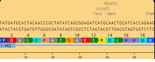 Figure 2. Snapshot from Benchling of MnSOD from DNA to Protein.
References
- Demicheli V, Moreno DM, Radi R. Human Mn-superoxide dismutase inactivation by peroxynitrite: a paradigm of metal-catalyzed tyrosine nitration in vitro and in vivo. Metallomics. 2018 May 23;10(5):679-695. doi: 10.1039/c7mt00348j.
- National Center for Biotechnology Information. Manganese superoxide dismutase, partial [Stylophora pistillata]. GenBank: AAX99423.1 [Internet]. 2005 [cited 2026 Feb 17]. Available from: https://www.ncbi.nlm.nih.gov/protein/AAX99423.1.
- UniProt Consortium. Superoxide dismutase (Fragment) OS=Stylophora pistillata OX=50429 GN=AWC38_SpisGene15259 PE=4 SV=1. UniProtKB A3KLM5 [Internet]. 2007 [cited 2026 Feb 17]. Available from: https://www.uniprot.org/uniprotkb/A3KLM5/entry.
- Rusconi G. Stylophora pistillata [image]. In: Sealifebase [Internet]. 2005 [cited 2026 Feb 17]. Available from: https://www.sealifebase.ca/summary/Stylophora-pistillata.html.
- Furla P, Richier S, Allemand D. Stylophora pistillata manganese superoxide dismutase mRNA, partial cds [Internet]. GenBank: AY916505.1; 2005 [cited 2026 Feb 17]. Available from: https://www.ncbi.nlm.nih.gov/nuccore/AY916505.1.
- Plotkin JB, Kudla G. Synonymous but not the same: the causes and consequences of codon bias. Nat Rev Genet. 2011 Jan;12(1):32-42. doi: 10.1038/nrg2899.
- Gustafsson C, Govindarajan S, Minshull J. Codon bias and heterologous protein expression. Trends Biotechnol. 2004 Jul;22(7):346-53. doi: 10.1016/j.tibtech.2004.04.006.
- Rosano GL, Ceccarelli EA. Recombinant protein expression in Escherichia coli: advances and challenges. Front Microbiol. 2014 Apr 17;5:172. doi: 10.3389/fmicb.2014.00172.
- GenScript. GenSmart™ Codon Optimization [Internet]. Piscataway (NJ): GenScript; 2026 [cited 2026 Feb 17]. Available from: https://www.genscript.com/gensmart-free-gene-codon-optimization.html.
- Green MR, Sambrook J. Molecular Cloning: A Laboratory Manual. 4th ed. Cold Spring Harbor (NY): Cold Spring Harbor Laboratory Press; 2012.
- Gregorio NE, Levine MZ, Oza JP. A User’s Guide to Cell-Free Protein Synthesis. Methods Protoc. 2019 Mar 20;2(1):24. doi: 10.3390/mps2010024.
- Silverman AD, Karim AS, Jewett MC. Cell-free gene expression: an expanded repertoire of applications. Nat Rev Genet. 2020 Mar;21(3):151-170. doi: 10.1038/s41576-019-0186-3.
- Alberts B, Johnson A, Lewis J, et al. Molecular Biology of the Cell. 6th ed. New York: Garland Science; 2014. Chapter 6: How Cells Read the Genome: From DNA to Protein.
- Black DL. Mechanisms of alternative pre-messenger RNA splicing. Annu Rev Biochem. 2003;72:291-336. doi: 10.1146/annurev.biochem.72.121801.161720.
Part 4: Prepare a Twist DNA Synthesis Order
After creating my Twist and Benchling account, I built my DNA insert sequence to make MnSOD (see [Figure 7,8]). I went through each piece of the DNA sequence and annotated the parts and finally got a Linear Map of the entire sequence [Figure 9]. Then on Twist, I imported the sequence by uploading the FASTA file from Benchling. Since the order is for a clonal gene, I had to then select a cloning vector like pTwist Amp High Copy. I then proceeded to download construct (GenBank) to get the full plasmid sequence and imported this to Benchling to see the plasmid with the expression cassette [Figure 10].
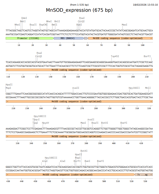 Figure 7. Annotations for MnSOD.
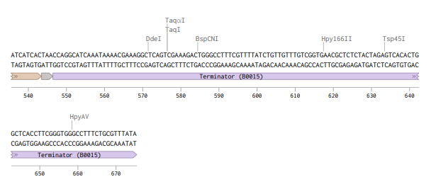 Figure 8. MnSOD annotations continued.
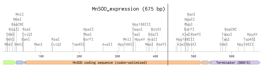 Figure 9. MnSOD Linear Map.
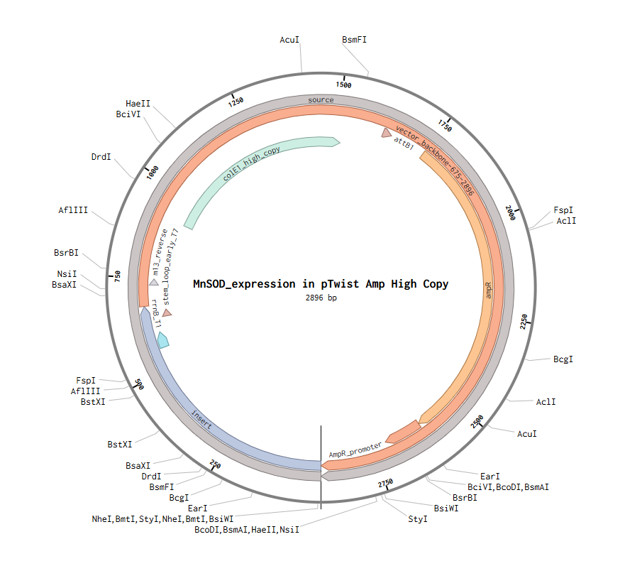 Figure 10. MnSOD plasmid with expression cassette.
Part 5: DNA Read/Write/Edit
DNA Read
(i) What DNA would you want to sequence (e.g., read) and why?
I would want to sequence environmental DNA (eDNA) from coral reef water samples around deployment sites of the biodegradable pods. If the MnSOD-producing bacteria where deployed on a reef, various factors would have to be monitored. The first factor would be whether the strain persists in the environment which eDNA sequencing from water samples could detect using the MnSOD gene itself [1]. Water samples collected at various distances from deployment sites would tell if containment is working by showing whether or not it has spread beyond the target area [1]. Additionally, coral-associated samples would reveal if introducing the probiotic is disrupting the natural microbial community [2].
(ii) In lecture, a variety of sequencing technologies were mentioned. What technology or technologies would you use to perform sequencing on your DNA and why?
I would use Illumina next-generation sequencing (NGS). [3,4] For eDNA metagenomics, the high throughput is essential for capturing the full diversity of microbial communities. Illumina’s short reads have very low error rates (around 0.1-1%) [5], which matters when confirming the gene sequence. Illumina also offers the best balance of data quality and price considering the scale of monitoring required in this specific case. This is a second-generation sequencing technology, and it’s defined by massively parallel sequencing, i.e. reading millions of short DNA fragments simultaneously instead of one at a time like Sanger sequencing [3,4]. The main difference between Sanger, which is first-generation, and Illumina, is the number of fragments read at one time. Sanger reads one fragment at a time [6,7], whilst Illumina can read millions of fragments in parallel [3,4]. Other distinctions include long reads up to 900 bp, slow and expensive but accurate for each base for Sanger [7] vs short reads of up to 300 bp, high accuracy and lower cost per base for Illumina [4]. Third generation methods like PacBio and Nanopore can achieve very long reads up to 100 kb or more but they have higher error rates [8,9].
The input for Illumina NGS would be the DNA extracted from filtered seawater samples or coral mucus swabs. The following are the preparation steps [1,10]:
- Filter large volumes of seawater to capture microbial biomass
- Extract total DNA (including human, fish, microbial, and free DNA)
- Quantify and check quality
- Fragmentation (mechanical or enzymatic)
- Adapter ligation with barcodes (to multiplex many samples)
- PCR amplification
- Library pooling
The first essential step of Illumina sequencing is the library preparation during which DNA is fragmented, and adapters are ligated to both ends [3,4]. Then, the library fragments must be attached to a flow cell surface. Bridge amplification creates thousands of identical copies of each fragment in tight clusters. Fluorescently labeled nucleotides would then be added one at a time. As each nucleotide incorporates, a camera takes an image of the flow cell. The color tells you which base (A, T, C, or G) was added. Then, a software analyzes the images, identifying which base was added to each cluster in each cycle. The sequence of colors across cycles gives you the DNA sequence for each fragment [3,4]. Finally, the millions of short reads are assembled and annotated. The output is then millions of short sequencing reads in FASTQ format, which is a text file containing a read identifier, the nucleotide sequence (A, T, C, G), and quality scores for each base (Phred scores) indicating the confidence in each call [11]. This would provide the community composition data which tells you which microbial species are present and in what relative abundances.
DNA Write
(i) What DNA would you want to synthesize (e.g., write) and why?
I want to synthesize a heat-sensing genetic circuit that could eventually be used to monitor coral reef health. The idea is to create bacteria that glow when the water gets too warm providing an early warning sign before corals start to bleach. The DNA I’d synthesize is a single construct containing two parts: a heat-shock promoter from a coral or its symbiotic algae, and a fluorescent protein gene (mCherry) that makes bacteria turn red. When the temperature rises, the promoter turns on, the bacteria produce mCherry, and they start to glow. If it’s possible to make bacteria that glow when the water changes temperature, then it would be possible to swap the mCherry gene for the MnSOD gene later and have bacteria that actually protect corals instead of just reporting on them [2].
The mCherry sequence I’m referring to is the standard version developed by Shaner et al. [12] and codon-optimized for E. coli expression based on the iGEM Parts Registry [13]. I have to find the exact promoter sequence from a coral database separately but the reporter part, the mCherry sequence, is the following:
ATGGTGAGCAAGGGCGAGGAGGATAACATGGCCATCATCAAGGAGTTCATGCGCTTCAAGGTGCACATGGAG GGCTCCGTGAACGGCCACGAGTTCGAGATCGAGGGCGAGGGCGAGGGCCGCCCCTACGAGGGCACCCAGACC GCCAAGCTGAAGGTGACCAAGGGTGGCCCCCTGCCCTTCGCCTGGGACATCCTGTCCCCTCAGTTCATGTAC GGCTCCAAGGCCTACGTGAAGCACCCCGCCGACATCCCCGACTACTTGAAGCTGTCCTTCCCCGAGGGCTTC AAGTGGGAGCGCGTGATGAACTTCGAGGACGGCGGCGTGGTGACCGTGACCCAGGACTCCTCCCTGCAGGAC GGCGAGTTCATCTACAAGGTGAAGCTGCGCGGCACCAACTTCCCCTCCGACGGCCCCGTAATGCAGAAGAAG ACCATGGGCTGGGAGGCCTCCTCCGAGCGGATGTACCCCGAGGACGGCGCCCTGAAGGGCGAGATCAAGCAG AGGCTGAAGCTGAAGGACGGCGGCCACTACGACGCTGAGGTCAAGACCACCTACAAGGCCAAGAAGCCCGTG CAGCTGCCCGGCGCCTACAACGTCAACATCAAGTTGGACATCACCTCCCACAACGAGGACTACACCATCGTG GAACAGTACGAACGCGCCGAGGGCCGCCACTCCACCGGCGGCATGGACGAGCTGTACAAGTAA
(ii) What technology or technologies would you use to perform this DNA synthesis and why?
I would use Twist Bioscience’s silicon-based DNA synthesis platform [14]. Twist synthesizes DNA by building short fragments on silicon chips and then assembling them into longer pieces. Their method is accurate, reliable, and perfect for a project like this where I only need one construct to start testing. First, I would design my sequence and upload it to Twist’s portal. Inside their machine, they synthesize short overlapping oligonucleotides adding one nucleotide at a time in a series of chemical cycles. Then they assemble those fragments into the full-length gene using PCR assembly, where the overlapping ends act like puzzle pieces that only fit together one way. Once the full gene is made, they insert it into a plasmid and transform it into E. coli. They grow up the bacteria, sequence the DNA to make sure it’s 100% correct, and then send me either the purified DNA or a tube of bacteria with my gene inside [14].
In terms of speed, it takes about 5-10 business days to get the DNA [14]. That’s fine for planning experiments but not something you’d use in an emergency. For accuracy, the chemistry isn’t perfect since each coupling step is about 99.5% efficient, meaning that for a 1000 bp gene, only about 1% of full-length products might be error-free. That’s why Twist sequences everything before shipping, so they only send out perfect clones. For scalability, Twist can make thousands of genes at once on their silicon chips but for a single gene like in my case, that doesn’t really matter. The main limitation for me would be cost.
DNA Edit
(i) What DNA would you want to edit and why?
Building on my project to engineer beneficial bacteria for coral reefs, I would want to edit two different targets: the MnSOD gene itself to create improved versions, and the genome of my engineered E. coli chassis to add biosafety features.
First, I would edit the MnSOD gene to test variants that might have higher activity or better stability. By introducing targeted mutations at specific amino acid positions, I could potentially create a superoxide dismutase enzyme that works more efficiently at the higher temperatures corals experience during bleaching events. This kind of protein engineering through gene editing is a common approach to improve enzyme function. Second, and more importantly for my project’s real-world application, I would edit the genome of my engineered E. coli strain to add a kill switch. In my Week 1 governance section, I discussed the importance of containment and preventing engineered bacteria from spreading uncontrollably in the environment. A kill switch is a genetic circuit designed to cause cell death under specific conditions, for example, if the bacteria escape the coral reef environment or if a certain time period has passed. This would address the ethical concerns I raised about disrupting native microbiomes and would make the whole approach much safer.
The specific edit would involve inserting a synthetic gene circuit into a neutral site in the E. coli chromosome. This circuit could be designed so that the bacteria require a synthetic amino acid or a specific chemical signal to survive. Alternatively, it could be a temperature-sensitive switch that kills the bacteria if they leave the warm reef waters. These kinds of biocontainment strategies are actively being developed in synthetic biology to address exactly the safety concerns I outlined in my earlier work [15].
(ii) What technology or technologies would you use to perform these DNA edits and why?
I would use CRISPR-Cas9 for both types of edits [16]. CRISPR is the most versatile and precise genome editing tool available, and it works well in E. coli which is my chassis organism. For editing the MnSOD gene on a plasmid, CRISPR-Cas9 would allow me to introduce specific point mutations efficiently. For the more complex task of inserting a kill switch into the bacterial chromosome, CRISPR is ideal because it can target a specific genomic location with high precision [17]. CRISPR-Cas9 works through a simple two-component system. The Cas9 protein is a nuclease that cuts DNA, and a guide RNA (gRNA) directs it to the right location [16].
There are five essential steps to CRISPR-Cas9. First, there needs to be a guide RNA with a 20-nucleotide sequence that matches my target site in the E. coli genome. The target site must be next to a PAM sequence (NGG for the standard Cas9 from Streptococcus pyogenes) which is required for Cas9 to bind. For the kill switch insertion, there would also need to be a donor DNA template which is the kill switch gene sequence flanked by homology arms that match the genomic target site [18]. Then, three components would be introduced into the E. coli cells: a plasmid expressing Cas9, a plasmid expressing the guide RNA, and the donor DNA template for insertion edits. This is typically done through electroporation, which uses an electric field to make cells temporarily permeable to DNA. Inside the cell, the guide RNA binds to Cas9 and directs it to the matching genomic sequence. Cas9 checks for the PAM sequence, unwinds the DNA, and if the match is good, it makes a double-strand break about three nucleotides upstream of the PAM [17]. Next, the cell’s natural repair systems kick in. Without a donor template, the break is repaired by non-homologous end joining (NHEJ), which is error-prone and often disrupts the gene. With a donor template present, the cell can use homology-directed repair (HDR) to copy the donor sequence into the genome, which is how I would insert my kill switch [18]. After editing, I would sequence the target region to confirm the edit worked correctly and that there were no off-target mutations.
For the kill switch insertion, the preparation steps would include:
- Designing the kill switch genetic circuit (promoter, toxin gene, regulator elements)
- Designing guide RNAs targeting a neutral integration site in the E. coli genome (sites like attTn7 that are known to tolerate insertions without disrupting essential genes)
- Designing and ordering the donor DNA template (the kill switch flanked by 500-1000 bp homology arms)
- Cloning the guide RNA into a suitable expression plasmid
- Preparing the Cas9 expression plasmid (or using a strain that already expresses Cas9)
- Preparing competent E. coli cells for transformation
The input materials would be: the two plasmids (Cas9 and gRNA), the donor DNA template (either as linear DNA or on a separate plasmid), and competent cells of my target strain [18].
CRISPR-Cas9 is powerful but has limitations. In terms of efficiency, homology-directed repair (HDR) is much less efficient than non-homologous end joining (NHEJ), especially in bacteria. For inserting a kill switch, only a small percentage of cells that take up the DNA will undergo the correct HDR event. This means I would need a good screening method to find the correct clones [17]. In terms of precision, CRISPR can sometimes cut at off-target sites that are similar but not identical to the intended sequence. This could introduce unwanted mutations elsewhere in the genome. Using high-fidelity Cas9 variants and carefully designing guide RNAs with unique targets can minimize this risk [16]. Another limitation is delivery. Getting all the components into cells efficiently can be challenging, especially for non-model organisms. For E. coli, electroporation works well, but for editing coral symbionts directly, delivery would be much harder. Finally, there’s the PAM requirement. Cas9 can only target sequences next to a PAM, which limits where I can edit. For my kill switch integration site, I would need to find a safe genomic location that also has a suitable PAM sequence nearby. Despite these limitations, CRISPR-Cas9 is still the best choice because it is precise, programmable, and has a huge research community developing improved versions and methods.
References
- Liles MR, Williamson LL, Rodbumrer J, Torsvik V, Goodman RM, Handelsman J. Isolation and Cloning of High-Molecular-Weight Metagenomic DNA from Soil Microorganisms. Cold Spring Harb Protoc. 2009;2009(8):pdb.prot5271.
- Gao B, Ruiz D, Case H, Jinkerson RE, Sun Q. Engineering bacterial warriors: harnessing microbes to modulate animal physiology. Curr Opin Biotechnol. 2024;87:103113.
- Illumina Inc. An Introduction to Next-Generation Sequencing Technology [Internet]. San Diego: Illumina; 2021 [cited 2026 Feb 17]. Available from: https://www.illumina.com/technology/next-generation-sequencing.html.
- Illumina Inc. HiSeq 4000 Sequencing System [Internet]. San Diego: Illumina; 2024 [cited 2026 Feb 17]. Available from: https://www.biocompare.com/23967-Next-Generation-Sequencers/11182181-HiSeq-4000-Sequencing-System/.
- De-Kloet RE, Jansen HJ, Groenen MAM, Megens HJ. Comparison of Pacific Biosciences (PacBio), Oxford Nanopore Technologies (ONT), Illumina (IL), 10× Genomics linked-read sequencing on the Illumina platform (10×), RNA sequencing on the Illumina platform (RNA-seq), BioNano Genomics (BNG) and the genome-wide chromatin conformation capture protocol Hi–C (Hi–C). [Table 3] In: Comprehensive comparison of long-read and short-read sequencing technologies for de novo genome assembly. 2020 [cited 2026 Feb 17]. Available from: https://pmc.ncbi.nlm.nih.gov/articles/PMC7925608/table/Tab3/.
- Thermo Fisher Scientific. How to Conduct Sanger Sequencing [Internet]. Waltham (MA): Thermo Fisher Scientific; 2025 [cited 2026 Feb 17]. Available from: https://www.thermofisher.com/hk/en/home/life-science/sequencing/sequencing-learning-center/capillary-electrophoresis-information/how-conduct-fragment-analysis0.html.
- University of British Columbia Sequencing and Bioinformatics Consortium. Sanger FAQ [Internet]. Vancouver: UBC; 2025 [cited 2026 Feb 17]. Available from: https://sequencing.ubc.ca/our-services-equipment/sanger-sequencing/sanger-faq.
- Yale School of Medicine. PacBio Single Molecule Real-Time (SMRT) Sequencing System [Internet]. New Haven: Yale University; 2024 [cited 2026 Feb 17]. Available from: https://dev.medicine.yale.edu/keck/microarray/services/long-reads-sequencing/pacbio/.
- Wang Y, Zhao Y, Bollas A, Wang Y, Au KF. Nanopore sequencing technology, bioinformatics and applications. Nat Biotechnol. 2021 Nov 8;39(11):1348-1365. doi: 10.1038/s41587-021-01108-x.
- Peabody MA, Hullahalli K, Sistu H, Pritchard JR, Walker S. Preparation of functional metagenomic libraries from low biomass samples using METa assembly and their application to capture antibiotic resistance genes. mSystems. 2025 Oct 21;10(10):e01039-25. doi: 10.1128/msystems.01039-25.
- Cock PJ, Fields CJ, Goto N, Heuer ML, Rice PM. The Sanger FASTQ file format for sequences with quality scores, and the Solexa/Illumina FASTQ variants. Nucleic Acids Res. 2010 Apr;38(6):1767-71. doi: 10.1093/nar/gkp1137.
- Shaner NC, Campbell RE, Steinbach PA, Giepmans BN, Palmer AE, Tsien RY. Improved monomeric red, orange and yellow fluorescent proteins derived from Discosoma sp. red fluorescent protein. Nat Biotechnol. 2004 Dec;22(12):1567-72.
- iGEM Foundation. mCherry coding sequence (BBa_J06504) [Internet]. 2022 [cited 2026 Feb 17]. Available from: http://parts.igem.org/Part:BBa_J06504.
- Twist Bioscience. DNA Synthesis Technology [Internet]. San Francisco: Twist Bioscience; 2026 [cited 2026 Feb 17]. Available from: https://www.twistbioscience.com/.
- Chan CTY, Lee JW, Cameron DE, Bashor CJ, Collins JJ. ‘Deadman’ and ‘Passcode’ microbial kill switches for bacterial containment. Nat Chem Biol. 2016 Feb;12(2):82-6. doi:10.1038/nchembio.1979.
- Jinek M, Chylinski K, Fonfara I, Hauer M, Doudna JA, Charpentier E. A programmable dual-RNA-guided DNA endonuclease in adaptive bacterial immunity. Science. 2012 Aug 17;337(6096):816-21. doi: 10.1126/science.1225829.
- Jiang W, Bikard D, Cox D, Zhang F, Marraffini LA. RNA-guided editing of bacterial genomes using CRISPR-Cas systems. Nat Biotechnol. 2013 Mar;31(3):233-9. doi: 10.1038/nbt.2508.
- Ran FA, Hsu PD, Wright J, Agarwala V, Scott DA, Zhang F. Genome engineering using the CRISPR-Cas9 system. Nat Protoc. 2013 Nov;8(11):2281-2308. doi: 10.1038/nprot.2013.143.
Week 3: Lab Automation
Python Script for Opentrons Artwork
Using the GUI at opentrons-art.rcdonovan.com I was able to generate a pattern to simulate the skyline at night in a desert (see Figure 1). LifeFabs Opentrons only has access to Blue, Pink, and Purple pigment which is why I decided to use these 3 colors only.
 Figure 1. Night sky in a desert (Automation Art Interference GUI).
The colors were achieved using eqFP578 (blue), TagRFP (pink), and mCherry (purple.)
Then, using the coordinates from the GUI, I followed the instructions in the HTGAA26 Opentrons Colab to write my own Python script with the assistance of Claude (Anthropic) which helped me structure the pipetting logic. This is the code:
The output is the following:
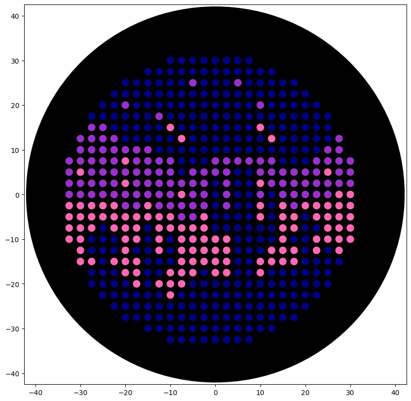 Figure 2. Night sky in a desert (Opentrons Colab).
Post-Lab Questions
- Find and describe a published paper that utilizes the Opentrons or an automation tool to achieve novel biological applications.
- Write a description about what you intend to do with automation tools for your final project. You may include example pseudocode, Python scripts, 3D printed holders, a plan for how to use Ginkgo Nebula, and more. You may reference this week’s recitation slide deck for lab automation details.
Final Project Ideas
This idea is ba continuation on the research I did for the homework in Weeks 1 and 2.

This idea came about after reading about the recent wildfires in Patagonia, Argentina and further researching recent wildfires across the world including Chile, Spain and Portugal. I started thinking about the ways that already exist to prevent wildfires and thought if there were any methods that use modified living organisms.
Because my background is in biomedical engineering I thought I should have at least one project idea that was related healthcare. Before starting my degree I did some research into bandaids made with hydrogels which act like stitches and prevent infection. Last summer, I did an internship which used microfluidics for blood glucose monitoring which made me think if there was any way I could combine microfluidics and something to improve wound care. That led me to chronic wounds and I began researching monitoring methods for these wounds that led me to biosensors for chronic wound management.
Post-lab Questions
- Find and describe a published paper that utilizes the Opentrons or an automation tool to achieve novel biological applications.
I read the following paper: “Semiautomated Production of Cell-Free Biosensors” (Brown DM, Phillips DA, Garcia DC, et al. ACS Synthetic Biology. 2025;14(3):979-986.)
The researchers used an Opentrons OT-2 to automate the assembly of cell-free biosensors. They compared manual vs. robotic assembly of biosensors that produce colorimetric (LacZ) or fluorescent (GFP) signals. Using the robot, they successfully constructed an entire 384-well plate of fluoride-sensing biosensors with consistent performance. They noted that manual assembly leads to quality control and performance variability issues. Their robotic workflow produced biosensors that performed close to expected detection outcomes proving that Opentrons can manufacture point-of-care diagnostic devices at scale.
- Write a description about what you intend to do with automation tools for your final project. You may include example pseudocode, Python scripts, 3D printed holders, a plan for how to use Ginkgo Nebula, and more. You may reference this week’s recitation slide deck for lab automation details.
For my Smart Scab project, I will use automation tools to manufacture and optimize cell-free biosensors that detect bacterial quorum sensing molecules. My plan has four main or potential components. Inspired by Brown et al.’s Semiautomated Production of Cell-Free Biosensors, I could use the OT-2 to assemble 384-well plates of cell-free reactions with different concentrations of quorum sensing molecules (AHLs for Pseudomonas, AIPs for S. aureus). This would allow me to generate full dose-response curves in 15 minutes rather than 3 hours manually. This is an example Pytho pseudocode:
Following the APEX workflow, I could use the OT-2 to automate screening of my designed fusion proteins (sensor domain + reporter). The pipeline would look something like:
- Heat shock transformation of variant libraries into E. coli (using OT-2 thermocycler module)
- Selective plating with automated agar height calculation (using the method from APEX: measuring density via pipette tip touch)
- Colony sampling to pick colonies for protein production
- Expression induction and lysis for testing
APEX’s spreadsheet-based configuration means I could run this without advanced coding skills, I simply fill CSV files with source wells and transfer volumes.
I would also design and 3D print several custom adapters, including an agar plate adapter, a hydrogel mold, and deck riser. The agar plate adapter positions 90 mm Petri dishes on the OT-2 deck for automated colony sampling (following APEX’s design). The hydrogel mold creates uniform 8 mm diameter, 2 mm thick alginate discs that fit into the patch housing, ensuring consistent sensor deposition. And the deck riser allows stacking multiple 384-well plates to increase throughput beyond the OT-2’s standard 4-plate capacity.
Finally, once my OT-2 protocols identify the best-performing protein variants, I would scale up using Ginkgo Cloud Lab. That would give me access to over 70 automated instruments including liquid handlers, incubators, and plate readers.
Week 4: Protein Design I
Part A: Conceptual Questions
1. How many molecules of amino acids do you take with a piece of 500 grams of meat? (on average an amino acid is ~100 Daltons)
A Dalton (Da), also known as an atomic mass unit, is a unit of mass that can be converted into grams (1 Dalton = 1 g/mol). To calculate the number of amino acid molecules, we first need the protein content. Assuming an average protein content in meat of approximately 22%, a 500-gram piece of meat contains about 110 grams of protein. Since 1 Dalton equals roughly 1.6605 × 10⁻²⁴ grams, and an average amino acid is 100 Da, a single amino acid molecule weighs approximately 1.66 × 10⁻²² grams. Therefore, the number of amino acid molecules in that meat is 110 grams divided by 1.66 × 10⁻²² grams, which is approximately 6.62 × 10²³ molecules.
2. Why do humans eat beef but do not become a cow, eat fish but do not become fish?
The proteins and other biomolecules in food are broken down during digestion into their basic building blocks (amino acids, sugars, fatty acids, etc.). These building blocks are then reassembled into human-specific proteins and structures according to our own genetic code. The information for building a cow or fish is not preserved, instead the nutrients are used for human metabolism and growth. Thus, we incorporate the material but not the form.
3. Why are there only 20 natural amino acids?
Amino acids are encoded by codons, which are sequences of three nucleotide bases. With four possible bases, there are 64 (4³) potential codon combinations. However, evolution has resulted in only 20 standard amino acids due to a phenomenon called “inherited redundancy,” where multiple codons specify the same amino acid. This redundancy makes the genetic code more robust by allowing for high-fidelity translation, as it minimizes the impact of mutations.
4. Can you make other non-natural amino acids? Design some new amino acids.
Yes, non-natural amino acids can be synthesized in the lab. For example, you could design an amino acid with a longer side chain, such as homophenylalanine (phenylalanine with an extra methylene group), or with a fluorinated side chain for enhanced stability. Another example is incorporating a photo-reactive group like azidophenylalanine. These can be introduced into proteins via methods like unnatural amino acid mutagenesis.
5. Where did amino acids come from before enzymes that make them, and before life started?
The Miller-Urey experiment in 1953 successfully demonstrated a potential origin for these molecules. They recreated the conditions thought to exist on primordial Earth by combining ammonia, hydrogen, methane, and water vapor in a flask and subjecting it to electrical sparks to simulate lightning (Miller, 1953). This experiment resulted in the formation of new organic molecules, which were identified as eleven of the standard amino acids. Thus, amino acids existed before life, providing the building blocks for the first proteins. As more complex life forms evolved, those that developed the metabolic pathways to synthesize their own amino acids gained a survival advantage. This is why modern organisms are capable of producing amino acids internally using enzymes.
6. If you make an α-helix using D-amino acids, what handedness (right or left) would you expect?
Natural α-helices are made of L-amino acids and are right-handed. D-amino acids are mirror images, so an α-helix made entirely of D-amino acids would be left-handed. This is because the chirality of the monomers dictates the helical twist.
8. Why are most molecular helices right-handed?
The right-handed α-helix is the predominant form in proteins due to the chirality of L-amino acids. Because L-amino acids are the building blocks, the helix forms a diastereomeric relationship where the right-handed conformation is energetically more stable. This stability was confirmed by Linus Pauling in his famous 1951 paper (although his original diagram actually showed a left-handed helix by mistake, as the absolute handedness of amino acids had only just been established). Modern quantum mechanical calculations show that right-handed helices are more stable by about 1 kcal/mol per residue due to optimized hydrogen bonding and fewer steric clashes.
9. Why do β-sheets tend to aggregate? What is the driving force for β-sheet aggregation?
β-sheets have extended conformations that expose backbone hydrogen-bonding groups. When multiple β-strands come together, they can form hydrogen bonds, leading to large aggregates. The hydrophobic side chains also contribute by minimizing contact with water, hence promoting stacking.
10. Why do many amyloid diseases form β-sheets? Can you use amyloid β-sheets as materials?
In amyloid diseases, like Alzheimer’s or Parkinson’s, proteins misfold into β-sheet-rich structures that are highly stable and resistant to degradation. Exposed edges readily latch onto other proteins using the same driving forces, hydrogen bonding and the hydrophobic effect, to form highly stable, insoluble aggregates or amyloid fibrils. This structure is so stable that the body’s normal machinery cannot break it down, leading to harmful buildup in tissues and disrupting cellular functions.
Researchers are now exploiting the extreme stability and self-assembling properties of amyloid β-sheets to create novel biomaterials. By designing peptides that form these structures, scientists can create nanowires, hydrogels, films, and scaffolds for applications in tissue engineering, biosensors, and even as templates for conducting materials. Their natural strength and ability to form ordered structures make them surprisingly useful.
Part B: Protein Analysis and Visualization
1. Briefly describe the protein you selected and why you selected it
I selected Heat shock protein 70 (HSP70-2) from the Egyptian fruit bat (Rousettus aegyptiacus). HSP70 is a molecular chaperone that helps other proteins fold correctly and prevents them from aggregating when cells are under stress, such as during high temperatures. I selected this protein because of my interest in ectotherms (animals that rely on external heat sources). Since ectotherms like reptiles and fish experience fluctuating body temperatures, their heat shock proteins must be particularly effective at protecting cells from temperature-induced damage. Understanding HSP70 provides insight into how organisms adapt to thermal stress at the molecular level.
2. Identify the amino acid sequence of your protein.
- How long is it? What is the most frequent amino acid? You can use this Colab notebook to count the frequency of amino acids.
- How many protein sequence homologs are there for your protein? Hint: Use Uniprot’s BLAST tool to search for homologs.
- Does your protein belong to any protein family?
This is the amino acid sequence for HSP70-2, UniProt ID: A0A7J8ILA0:
tr|A0A7J8ILA0|A0A7J8ILA0_ROUAE Heat shock-related 70 kDa protein 2 OS=Rousettus aegyptiacus OX=9407 PE=3 SV=1 MSARGPAIGIDLGTTYSCVGVFQHGKVEIIANDQGNRTTPSYVAFTDTERLIGDAAKNQVAMNPTNTIFDAKRLIGRKFEDATVQSDMKHWPFRVVSEGGKPKVQVEYKGEIKTFFPEEISSMVLTKMKEIAEAYLGGKVQSAVITVPAYFNDSQRQATKDAGTITGLNVLRIINEPTAAAIAYGLDKKGCAGGEKNVLIFDLGGGTFDVSILTIEDGIFEVKSTAGDTHLGGEDFDNRMVSHLAEEFKRKHKKDIGPNKRAVRRLRTACERAKRTLSSSTQASIEIDSLYEGVDFYTSITRARFEELNADLFRGTLEPVEKALRDAKLDKGQIQEIVLVGGSTRIPKIQKLLQDFFNGKELNKSINPDEAVAYGAAVQAAILIGDKSENVQDLLLLDVTPLSLGIETAGGVMTPLIKRNTTIPTKQTQTFTTYSDNQSSVLVQVYEGERAMTKDNNLLGKFDLTGIPPAPRGVPQIEVTFDIDANGILNVTAADKSTGKENKITITNDKGRLSKDDIDRMVQEAERYKSEDEANRDRVAAKNAVESYTYNIKQTVEDEKLRGKISEQDKNKILDKCQEVINWLDRNQMAEKDEYEHKQKELERVCNPIISKLYQGGPGGGGSGASGGPTIEEVD
Using the Colab notebook, the sequence length was 635 amino acids and this is the list of amino acid frequencies with G being the most common as it appears 55 times:
- G: 55
- K: 52
- A: 49
- E: 49
- I: 47
- T: 47
- D: 45
- L: 44
- V: 42
- S: 33
- R: 32
- N: 31
- Q: 27
- P: 22
- F: 21
- Y: 16
- M: 10
- H: 6
- C: 5
- W: 2
To identify homologs, I used UniProt’s BLAST tool. I entered the HSP70-2 sequence (UniProt ID: A0A7J8ILA0) and searched against the UniProtKB database. The search returned 250 homologous sequences, consisting of 5 reviewed (Swiss-Prot) entries and 245 unreviewed (TrEMBL) entries. The high number of homologs reflects how ancient and evolutionarily conserved the HSP70 family is across different organisms. Most homologs showed high sequence identity (92-100%), indicating strong evolutionary pressure to maintain the protein’s structure and function as a molecular chaperone.
Next, I examined the ‘Family & Domains’ section on the UniProt page for HSP70-2 to find out if it belonged to any protein family. The protein belongs to the Heat shock protein 70 family, characterized by conserved nucleotide-binding and substrate-binding domains. These features are consistent across all HSP70 proteins and explain their conserved function as molecular chaperones.
3. Identify the structure page of your protein in RCSB
- When was the structure solved? Is it a good quality structure? Good quality structure is the one with good resolution. Smaller the better (Resolution: 2.70 Å)
- Are there any other molecules in the solved structure apart from protein?
- Does your protein belong to any structure classification family?
For the 3D structure analysis, I initially searched for the bat HSP70-2 (UniProt ID: A0A7J8ILA0) in the RCSB PDB, but no experimentally solved structure was available for this specific protein. Therefore, I used the structure of the human HSP70-2 ATPase domain (PDB ID: 3I33), which can be found at: https://www.rcsb.org/structure/3i33, as a representative model. This is scientifically valid because HSP70 proteins are highly conserved across species as my BLAST search showed a >92% identity between species. Additionally, the functional domains (ATPase domain and substrate-binding domain) are nearly identical in structure across mammals. While not identical, the human structure serves as an excellent proxy to understand the 3D architecture of the HSP70 family, and it should provide meaningful insights into how the bat protein likely folds and functions. The amino acid sequence is the following:
3I33_1|Chain A|Heat shock-related 70 kDa protein 2|Homo sapiens (9606) MHHHHHHSSGVDLGTENLYFQSMPAIGIDLGTTYSCVGVFQHGKVEIIANDQGNRTTPSYVAFTDTERLIGDAAKNQVAMNPTNTIFDAKRLIGRKFEDATVQSDMKHWPFRVVSEGGKPKVQVEYKGETKTFFPEEISSMVLTKMKEIAEAYLGGKVHSAVITVPAYFNDSQRQATKDAGTITGLNVLRIINEPTAAAIAYGLDKKGCAGGEKNVLIFDLGGGTFDVSILTIEDGIFEVKSTAGDTHLGGEDFDNRMVSHLAEEFKRKHKKDIGPNKRAVRRLRTACERAKRTLSSSTQASIEIDSLYEGVDFYTSITRARFEELNADLFRGTLEPVEKALRDAKLDKGQIQEIVLVGGSTRIPKIQKLLQDFFNGKELNKSINPDEAVAYGAAVQAAILIGD
The length of the protein is 404 aminoacids and the most common amino acid remains G, which appears 36 times. These are the amino acid frequencies:
- G: 36
- A: 35
- K: 30
- T: 29
- I: 29
- L: 28
- E: 28
- V: 27
- D: 26
- S: 22
- R: 20
- F: 19
- N: 16
- Q: 14
- H: 12
- P: 12
- Y: 10
- M: 7
- C: 3
- W: 1
The entry title is “Crystal structure of the human 70kDa heat shock protein 2 (Hsp70-2) ATPase domain in complex with ADP and inorganic phosphate.” The structure was deposited in the Protein Data Bank on 2009-06-30 and released on 2009-07-21. It is a good quality structure as it was solved using X-ray diffraction to a resolution of 1.30 Å. This is well below the 2.70 Å threshold, meaning the atomic positions are determined with very high precision and confidence.
The structure contains several additional molecules bound to the protein [see Figure 1 below]. These include:
- ADP (Adenosine-5’-diphosphate): The nucleotide product remaining after the protein uses energy from ATP.
- PO4 (Phosphate ion): Released during the breakdown of ATP.
- MG (Magnesium ion): A crucial cofactor that helps bind the nucleotide.
- GOL (Glycerol): A molecule often used in the crystallization process.
- HOH (Water molecules): Hundreds of water molecules are part of the crystal structure.
 Figure 1. Chain A of human 70kDa heat shock protein 2 (Hsp70-2)
The ATPase domain of HSP70-2 belongs to several structure classification families. According to the RCSB PDB annotations for 3I33:
SCOPe classification: Class: Alpha and beta proteins (a/b); Fold: Ribonuclease H-like motif; Superfamily: Actin-like ATPase domain; Family: Actin/HSP70
CATH classification: 3.30.420.40 (Nucleotidyltransferase domain 5), 3.30.30.30 (Defensin A-like), and 3.90.640.10 (Actin, Chain A domain 4)
ECOD classification: Family PF00012 (Hsp70 protein family)
These classifications confirm that this domain shares a common evolutionary origin with actin and other ATPases, which is consistent with its function of binding and hydrolyzing ATP to drive protein folding.
4. Open the structure of your protein in any 3D molecule visualization software:
- PyMol Tutorial
- Visualize the protein as “cartoon”, “ribbon” and “ball and stick”.
- Color the protein by secondary structure. Does it have more helices or sheets?
- Color the protein by residue type. What can you tell about the distribution of hydrophobic vs hydrophilic residues?
- Visualize the surface of the protein. Does it have any “holes” (aka binding pockets)?
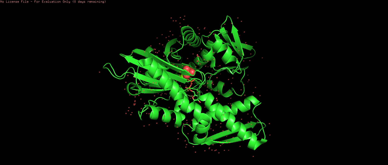 Figure 2. Default representation of the HSP70-2 ATPase domain (3I33) in PyMOL before any styling changes.
The initial view of the protein (PDB ID: 3I33) in PyMOL shows the default representation.
 Figure 3. Cartoon representation of HSP70-2 ATPase domain, showing alpha helices (spirals) and beta strands (arrows).
The cartoon representation highlights the secondary structure elements: alpha helices are shown as coiled ribbons, and beta sheets as flat arrows. This view makes it easy to see the overall fold and arrangement of structural motifs.
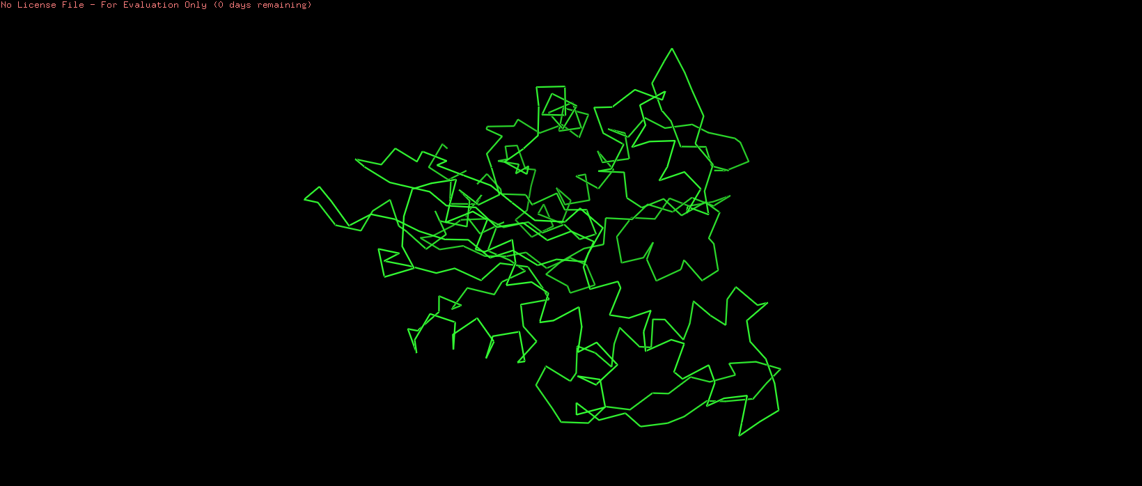 Figure 4. Ribbon representation of the HSP70-2 ATPase domain, illustrating the protein backbone trajectory.
The ribbon representation traces the protein backbone as a smooth, continuous ribbon, emphasizing the path of the polypeptide chain. Unlike the cartoon, it does not distinguish between helix and sheet but provides a clean, elegant view of the overall topology.
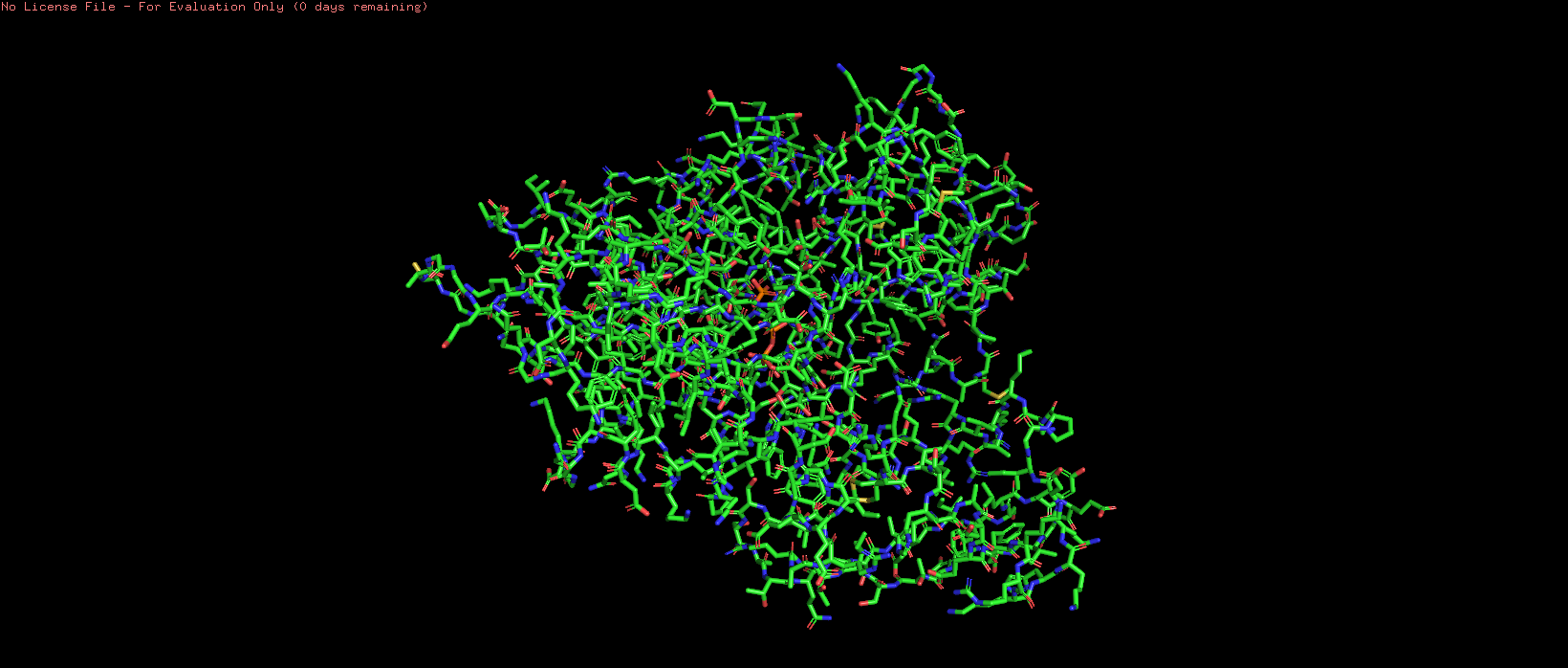 Figure 5. Ball and stick representation of HSP70-2, showing individual atoms and bonds.
The ball and stick representation shows individual atoms as spheres and bonds as sticks, revealing the detailed atomic structure. This view is particularly useful for examining side chain orientations and interactions within the active site.
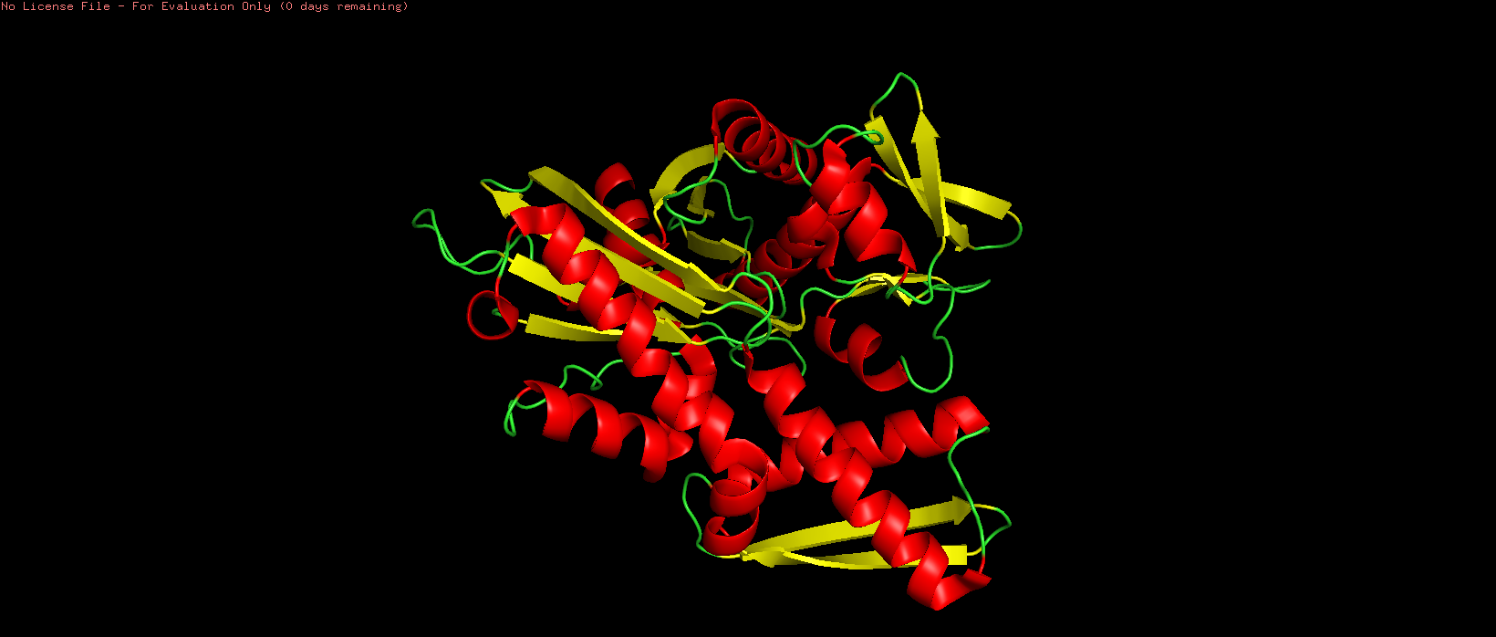 Figure 6. HSP70-2 ATPase domain colored by secondary structure (red = alpha helix, yellow = beta sheet, green = loop).
The protein is colored by secondary structure: alpha helices in red, beta sheets in yellow, and loops/turns in green. This color scheme clearly distinguishes the different secondary structure elements and their distribution throughout the domain. Based on the atom count from PyMOL, there are 1,368 atoms in alpha helices and 845 atoms in beta sheets. Therefore, the HSP70-2 ATPase domain contains more alpha helices than beta sheets. This is consistent with the structure of the actin-like ATPase fold, where helices surround a central beta-sheet core.
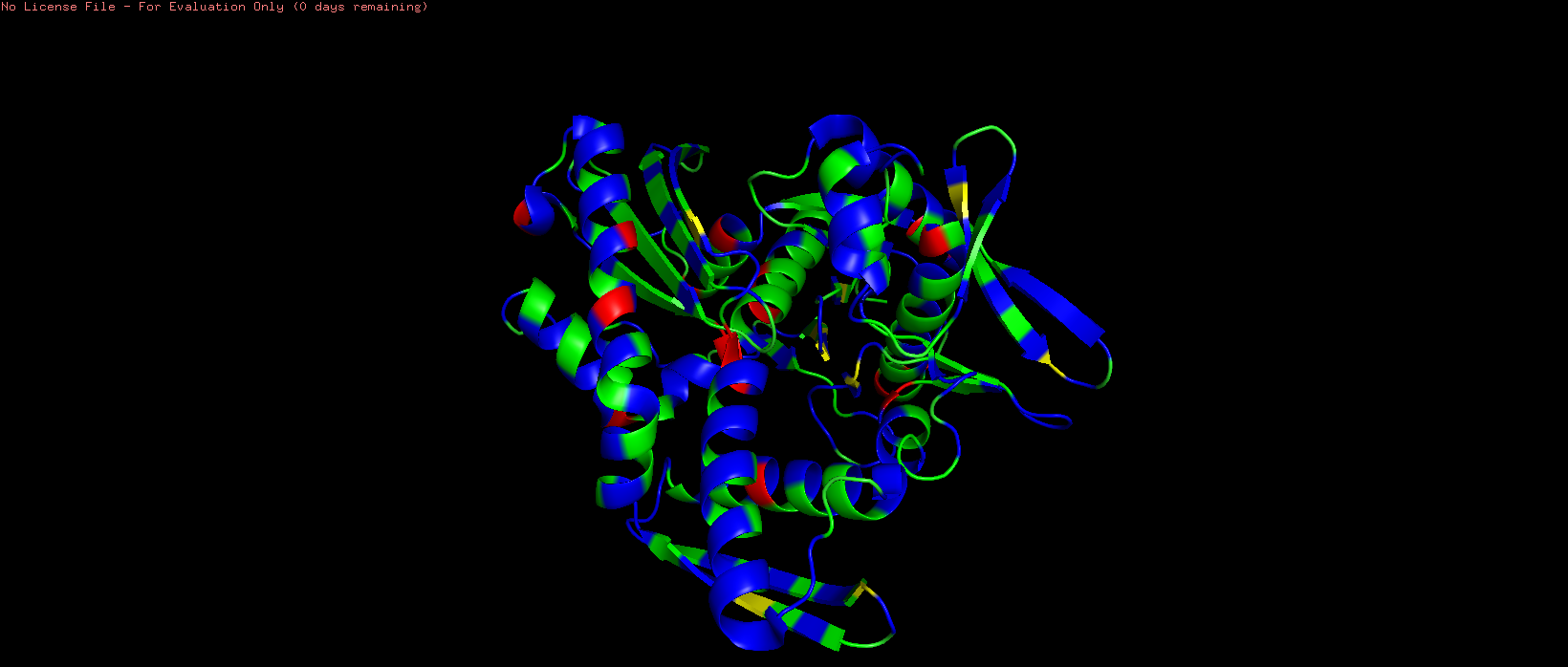 Figure 7. HSP70-2 ATPase domain colored by residue hydrophobicity (red = most hydrophobic, blue = hydrophilic).
The protein is colored by residue type using the Eisenberg hydrophobicity scale, where hydrophobic residues (Ile, Leu, Val, Phe, Trp, Met, Ala) appear in shades of red and orange, while hydrophilic residues (charged and polar amino acids) appear in shades of white and blue. This color scheme reveals that hydrophobic residues are predominantly buried within the protein core, while hydrophilic residues are more exposed on the surface. The distribution of hydrophobic and hydrophilic residues follows the typical pattern of a soluble globular protein. Hydrophobic residues (Ile, Leu, Val, Phe, Trp, Met, Ala) are primarily located in the interior of the protein, forming a stable hydrophobic core that drives proper folding through the hydrophobic effect . In contrast, hydrophilic residues (Arg, Lys, Asp, Glu, Asn, Gln, Ser, Thr) are predominantly exposed on the protein surface, where they can interact favorably with the surrounding water molecules. This arrangement is essential for protein solubility and stability. Interestingly, the nucleotide-binding pocket contains a mix of both hydrophobic and hydrophilic residues.
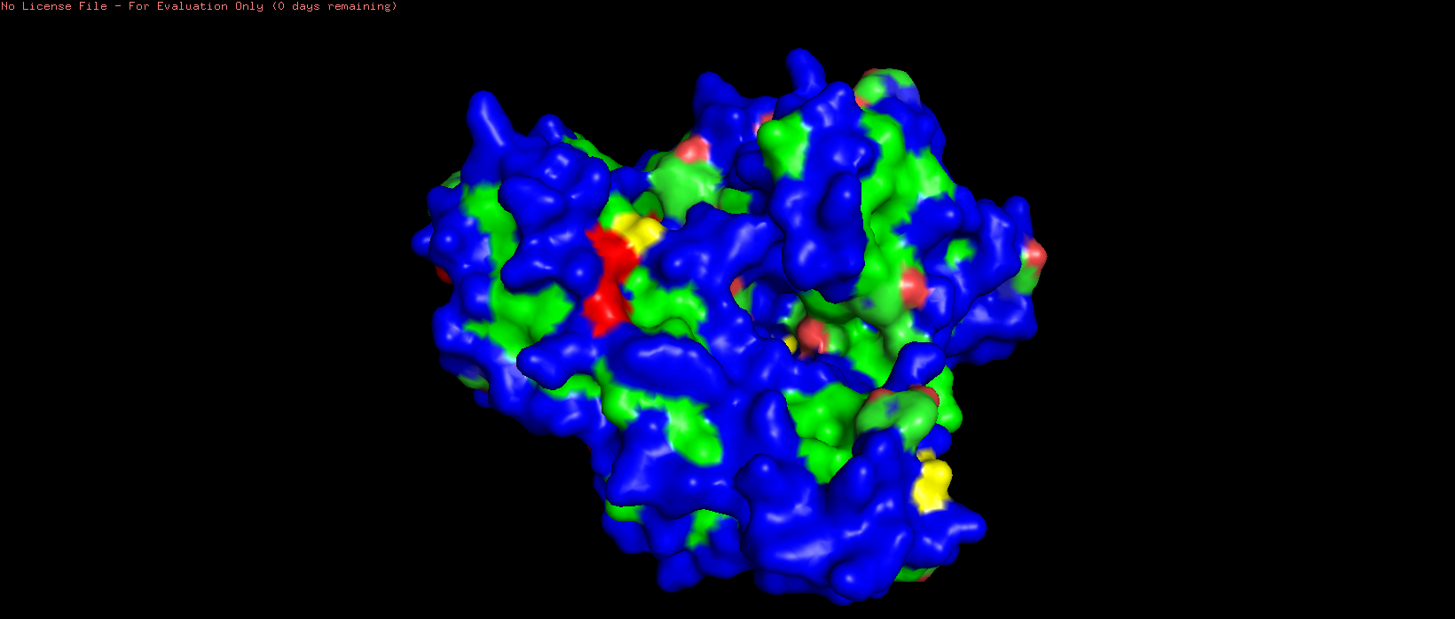 Figure 8. Surface representation of HSP70-2 ATPase.
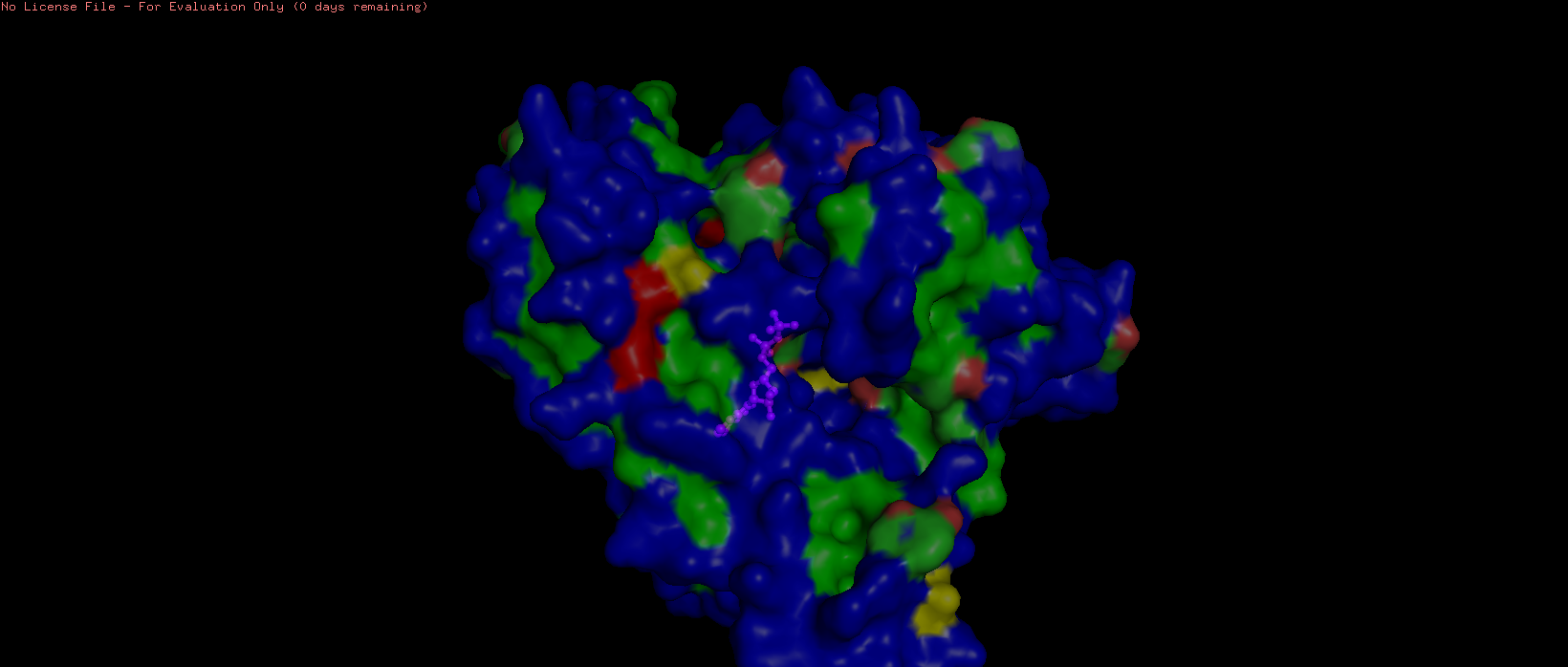 Figure 9. Surface representation of HSP70-2 ATPase domain showing the ADP in magenta (sticks and spheres) at transparency 0.5.
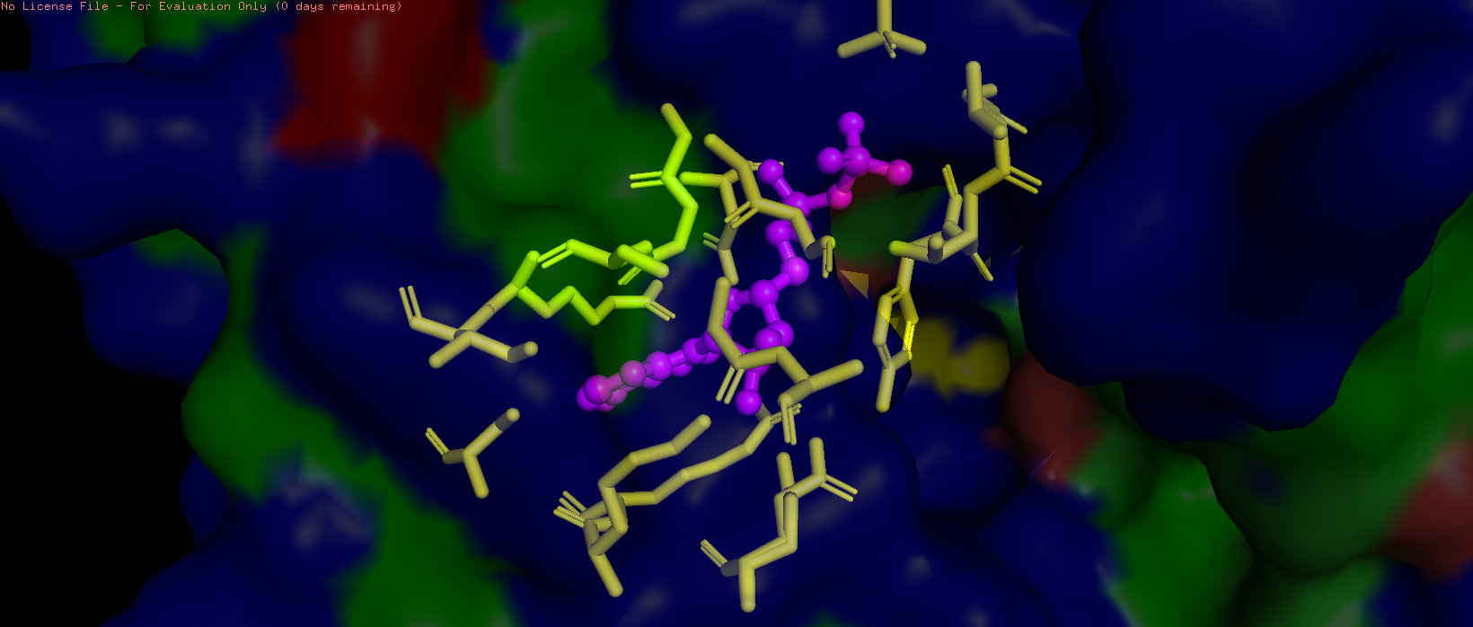 Figure 10. Pocket residues within 4.2 Å of ADP are highlighted in yellow.
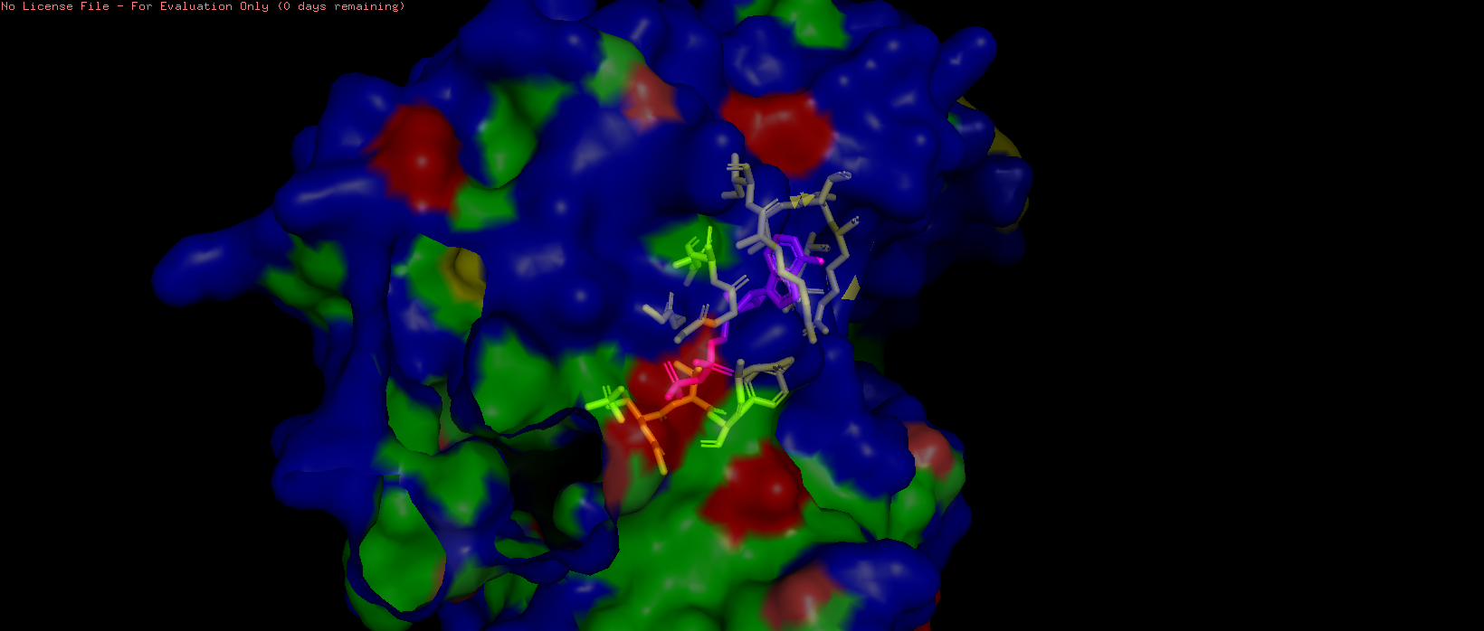 Figure 11. Surface representation of HSP70-2 ATPase domain showing the ADP-binding pocket (transparency = 0.5).
The HSP70-2 ATPase domain contains a prominent binding pocket that accommodates ADP. This pocket is located in the deep cleft between subdomains I and II of the ATPase domain. The pocket is lined with specific residues that coordinate nucleotide binding. The adenine ring binds in a hydrophobic region formed by residues such as Ile, Leu, and Val. The ribose and phosphate groups interact with polar and charged residues including Asp, Glu, and Lys. A magnesium ion is coordinated within the pocket to assist with phosphate binding. The presence of this pocket is functionally critical, as HSP70 proteins hydrolyze ATP to provide energy for their chaperone activity helping other proteins fold correctly. Additional small molecules in the structure, including glycerol (GOL) and phosphate ions (PO4), are also bound near the pocket, further confirming its role as the primary ligand-binding site.
Part C. Using ML-Based Protein Design Tools
C1. Protein Language Modeling
- Deep Mutational Scans
a. Use ESM2 to generate an unsupervised deep mutational scan of your protein based on language model likelihoods. b. Can you explain any particular pattern? (choose a residue and a mutation that stands out) c. (Bonus) Find sequences for which we have experimental scans, and compare the prediction of the language model to experiment.
I used ESM2 (esm2_t33_650M_UR50D) to perform an unsupervised deep mutational scan of the HSPA2 ATPase domain (PDB: 3I33). For each position in the 380-residue sequence, the model masked that position and computed the log-likelihood ratio (LLR) of each possible amino acid substitution relative to the wild-type residue. A negative LLR indicates the mutation is disfavored by the language model (predicted deleterious), while a positive LLR indicates the substitution may be tolerated or even preferred.
The heatmap reveals a heterogeneous conservation landscape. Most positions show moderate tolerance (blue-green, LLR ~0 to -5), but a subset of columns reach the most extreme negative scores (LLR approaching -20, deep purple), indicating near-complete intolerance to any mutation. Notably, these highly constrained columns are scattered across the sequence rather than forming one continuous block. This is consistent with the known architecture of the Hsp70 ATPase domain, where the nucleotide-binding site is assembled from multiple loops that are distant in sequence but converge in three-dimensional space. The P (proline) row is among the darkest across most columns. This is a universal feature of protein mutational landscapes. Proline introduces a rigid kink in the backbone and eliminates the NH hydrogen bond donor, making it disruptive nearly everywhere except positions that naturally accommodate it. A region in the middle of the sequence shows a streak of yellow, indicating a position where ESM2 actually prefers a different amino acid over the wild-type. This likely corresponds to a surface-exposed, variable loop where natural Hsp70 homologs show sequence diversity, and the language model has learned that alternative residues are more common at this position across evolution. Among the most striking individual mutations in the scan is any substitution at the conserved Glycine within the Walker A motif (GIDLGTTYSCVGxxGKT). The G→P mutation at this position is predicted to be among the most deleterious in the entire protein (approaching LLR = -20). This is mechanistically justified since the P-loop Glycine requires backbone flexibility to adopt the conformation that cradles the phosphate groups of ADP/ATP. Proline would rigidly lock this backbone, directly disrupting nucleotide binding. The 3I33 crystal structure, which captures HSPA2 in complex with ADP and inorganic phosphate, shows this glycine positioned directly adjacent to the bound ligand, confirming its functional importance.
- Latent Space Analysis
a. Use the provided sequence dataset to embed proteins in reduced dimensionality. b. Analyze the different formed neighborhoods: do they approximate similar proteins? c. Place your protein in the resulting map and explain its position and similarity to its neighbors.
I used the SCOP ASTRAL database (release 2.08, 40% sequence identity cutoff) as my sequence dataset, which contains ~15,000 diverse protein sequences spanning the known structural universe. Sequences were embedded using ESM2 and reduced to 3D using t-SNE for visualization. The notebook as provided would have taken an estimated 41 hours to run on the full SCOP dataset using the esm2_t33_650M_UR50D model (650 million parameters), processing sequences one by one on a free Colab T4 GPU. Two modifications were made to make this computationally feasible. Instead of embedding all ~15,000 SCOP sequences, I randomly subsampled 500 sequences (random seed=42 for reproducibility), then appended my protein of interest (HSPA2, 3I33) as the 501st sequence to ensure it would appear in the final map. This reduced runtime from ~41 hours to ~30 seconds. I also switched from esm2_t33_650M_UR50D to esm2_t6_8M_UR50D (8 million parameters) for the embedding step. The smaller model produces 320-dimensional embeddings vs 1280-dimensional, and is substantially faster per sequence. Random subsampling means the neighborhood of any given protein depends partly on which 500 sequences happened to be drawn, a different random sample would produce a somewhat different map and potentially different nearest neighbors. The smaller model captures less nuanced sequence information than the 650M model, which may reduce the biological precision of the clustering. These are important caveats to keep in mind when interpreting the results. For a more rigorous analysis, one would embed the full dataset with the larger model, which would require either a more powerful GPU or batch processing overnight.
This is the plot produced by the original notebook code, where each dot represents one protein sequence and color corresponds to the value of the third t-SNE component (TSNE3), ranging from deep purple (most negative) to yellow (most positive). This coloring does not represent any biological annotation, it is purely geometric, showing how proteins are distributed along the third axis of the reduced space. The plot shows a broad, continuous cloud of ~500 proteins with some denser and sparser regions, and a general gradient from purple at the bottom to yellow at the top reflecting the TSNE3 axis.
Because the original plot gave no way to locate my specific protein among 501 identical-looking dots, I modified the visualization code with help from Claude to highlight HSPA2 in red while all other SCOP proteins remain blue. This makes it immediately clear where HSPA2 sits in the embedding landscape relative to the broader protein universe.
HSPA2 (red dot) is positioned in the lower-middle region of the point cloud, slightly towards the periphery of a local cluster rather than at the center of the overall distribution. It is not completely isolated, there are several blue dots nearby, but it is not buried deep inside a dense cluster either. This peripheral positioning is biologically sensible since the Hsp70 ATPase domain has a distinctive and ancient fold that is structurally shared with many proteins, but the specific human Hsp70 sequence is quite distinct from most other proteins in the randomly sampled SCOP set, naturally placing it somewhat away from the main mass. By hovering over the dots nearest to HSPA2 in the interactive Plotly plot, the closest neighbor was identified as d2w40a2, a protein from Plasmodium falciparum (the malaria parasite) classified under SCOP fold c.55.1, which is the Actin/HSP70 family. The Hsp70 ATPase domain belongs to the actin-like ATPase superfamily, a deeply conserved structural fold shared across actin, hexokinase, sugar kinases, and Hsp70 chaperones across all domains of life. The fact that ESM2 places human HSPA2 nearest to a P. falciparum protein from the same SCOP superfamily without ever being told anything about protein folds, structures, or taxonomy demonstrates that the language model has learned genuine evolutionary and structural relationships purely from patterns in protein sequences. The model has effectively rediscovered that these two proteins, despite coming from organisms separated by over a billion years of evolution, share a common ancestral fold. This validates the core premise of protein language model embeddings, proximity in embedding space approximates biological relatedness. The neighborhoods formed in the t-SNE map do approximate genuinely similar proteins, at least at the level of fold superfamily.
C2. Protein Folding
- Fold your protein with ESMFold. Do the predicted coordinates match your original structure?
ESMFold is a protein structure prediction model developed by Meta AI that predicts 3D protein structure directly from sequence using a large language model (ESM2) as its backbone, without requiring multiple sequence alignments. It outputs per-residue confidence scores called pLDDT (predicted local distance difference test, 0–100) and a global pTM score (predicted template modelling score, 0–1). Higher is better: pLDDT >90 and pTM >0.9 indicate very high confidence predictions.
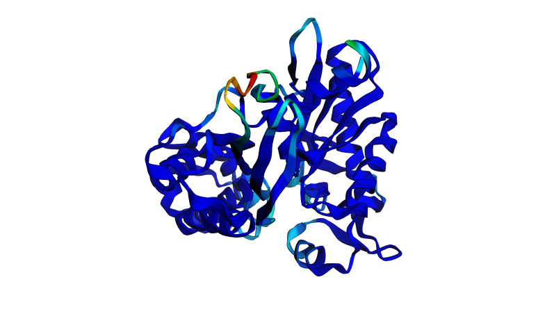
The ESMFold prediction of the wild-type HSPA2 ATPase domain is overwhelmingly deep blue, indicating very high confidence across nearly the entire structure. The characteristic two-lobe architecture of the Hsp70 ATPase domain is clearly visible, the large beta-sheet sandwich and surrounding alpha helices are all well-resolved. The only regions of lower confidence (cyan, green, yellow, red) are a small exposed loop near the nucleotide-binding cleft, which makes sense because this loop is flexible in solution and adopts slightly different conformations in different crystal structures. The ptm is 0.906 and pLDDT is 91.456. The predicted structure matches the known crystal structure (PDB: 3I33) very well. The overall fold, the relative orientation of the two subdomains, and the positions of the major secondary structure elements are all consistent with the experimentally determined coordinates.
- Try changing the sequence, first try some mutations, then large segments. Is your protein structure resilient to mutations?
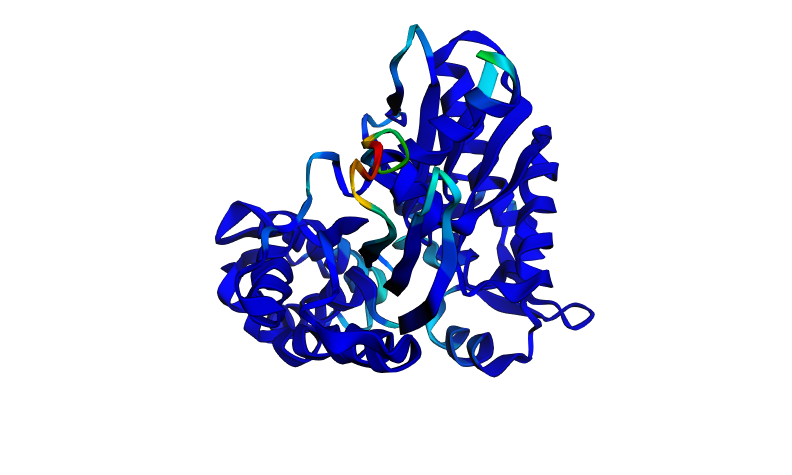
Two mutations were introduced at the most functionally critical residues identified from the ESM2 deep mutational scan: the P-loop glycine (G8A) and the Walker B catalytic aspartate (D→A). These are positions where the DMS scan predicted the most extreme fitness defects, with log-likelihood ratios approaching -20. Strikingly, the predicted structure is almost identical to the wild-type, the ptm score is unchanged (0.906) and the pLDDT drops by only 0.096 points (91.456 → 91.360), which is essentially negligible. The overall fold is completely preserved, with the same small flexible loop showing reduced confidence.
This reveals an important distinction, ESMFold predicts structure, not function. The mutations G8A and D→A are predicted by ESM2 to be severely deleterious to protein fitness, and experimentally they abolish ATPase activity entirely. However, they do not unfold the protein, the backbone scaffold of the ATPase domain is stable enough to maintain its fold even without these catalytic residues. This is a classic example of the difference between structural stability and functional activity. The protein retains its shape but loses its ability to hydrolyse ATP.
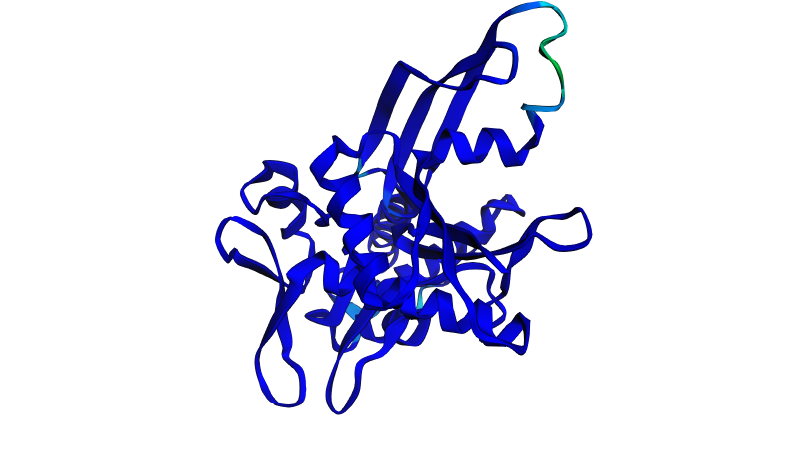
A stretch of about 97 residues was deleted from the middle of the sequence, removing part of the interdomain region and the Walker B motif. The result is surprising in that both confidence scores actually improved relative to wild-type (pTM 0.906 → 0.937, pLDDT 91.456 → 95.169), and the structure is almost entirely deep blue with almost no low-confidence regions.
I believe the deleted region included the most flexible loop that was responsible for the low-confidence (red/yellow) region in the wildtype prediction. By removing those residues, ESMFold no longer has to model a disordered, flexible region, so the truncated protein is a more compact, more rigidly foldable domain. The higher confidence scores reflect that the remaining sequence folds very cleanly into a stable structure, not that the deletion is biologically beneficial. However, this truncated protein would almost certainly be non-functional since it is missing critical structural and catalytic elements.
Across all three runs, HSPA2 demonstrates remarkable structural resilience. Point mutations at even the most functionally critical residues do not disrupt the predicted fold, and even a large deletion produces a confident prediction of a compact structure. This reflects the general principle that protein folds are often more tolerant of sequence change than protein functions.
C3. Protein Generation
- Analyze the predicted sequence probabilities and compare the predicted sequence vs the original one.
Traditional protein folding asks: given a sequence, what is the structure? Inverse folding asks the opposite: given a structure (backbone coordinates), what sequences would fold into it? ProteinMPNN is a graph neural network trained to take the 3D backbone geometry of a protein as input and outputs a probability distribution over amino acids at each position, then samples a new sequence predicted to fold into that same structure. This is a powerful tool for protein design because it allows generation of novel sequences with a desired fold.
I used ProteinMPNN (v_48_020, 48 edges, 0.20Å backbone noise) with the experimentally determined crystal structure of HSPA2 (PDB: 3I33) as input. Settings used:
- Designed chain: A (the full ATPase domain)
- Fixed chain: none
- Sampling temperature: 0.1 (low temperature — sequences stay close to natural amino acid preferences for that backbone)
- Number of sequences: 1
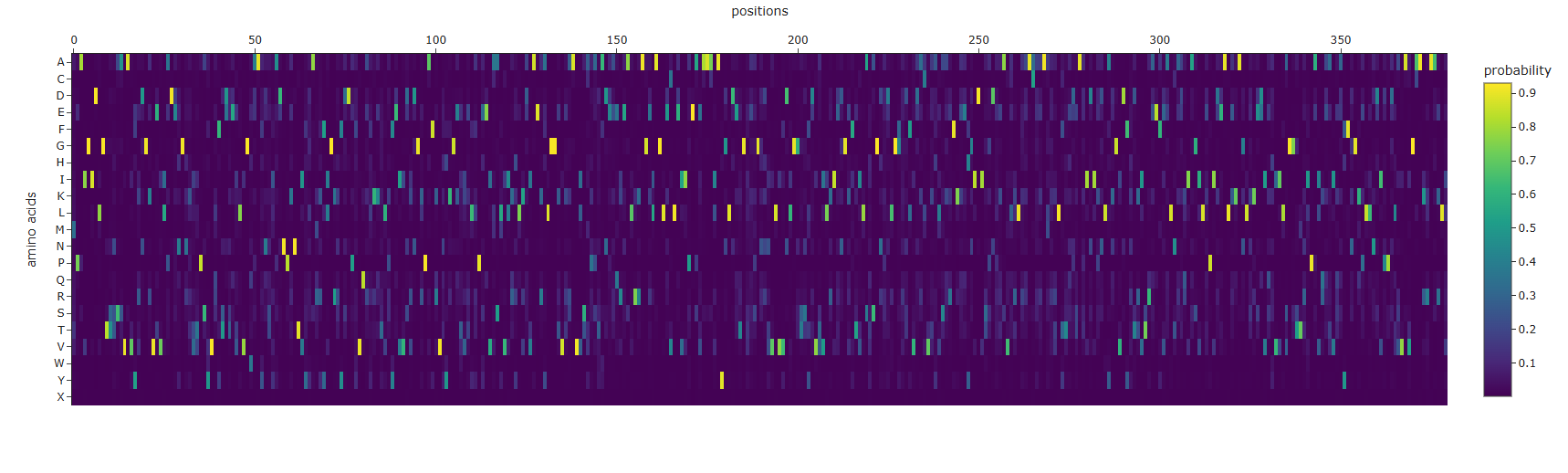
This heatmap shows ProteinMPNN’s predicted probability for each of the 20 amino acids (Y-axis) at every position in the protein (X-axis, positions 0–380). Color ranges from dark purple (probability = 0) to bright yellow (probability = 1).
Most positions have one clear dominant amino acid, at any given column, typically only one or two rows light up with yellow/green while everything else is dark purple. This means ProteinMPNN is highly confident about what amino acid belongs at most positions given the backbone geometry. This makes sense for a well-structured, deeply buried domain like the Hsp70 ATPase fold. Some positions show broader distributions, a handful of columns show multiple amino acids with moderate probabilities (cyan/teal across several rows). These correspond to surface-exposed positions where the backbone geometry is compatible with several different amino acids, reflecting genuine sequence flexibility at those sites. The G row (Glycine) lights up sharply at specific positions, and it is uniquely required wherever the backbone adopts conformations outside the normal Ramachandran space (e.g. tight turns, the P-loop). The L, I, V rows (hydrophobic residues) dominate the core positions, many of the brightest yellow cells are in the L, I, K, and V rows, reflecting the hydrophobic core of the ATPase domain where bulky nonpolar residues are structurally required.
ProteinMPNN generated the following new sequence from the HSPA2 backbone:
MPAIGIDLGTGTSAVAVYRDGRVEVLADEHGNKTIPSYVRFTETEVLVGWDAYNSIADNPKNTIYGARKFLGR KFDDPYVQELKKTLKFKVVDVDGEPYFEVYYKGKTVTLRPEEVLALVIRRLVEVAERALGGTVRRAVITAPAD ADEEEREALRRAGELAGLEVLEIIPEPVAAAIAYGLDETGTEPGNKNVLVVDLGTSSFDVVILRIENGEFTILAVS GDRDLGFNNFVDALVKYLSEKFKKDYGIDITPDEKAVLTLKKAAAKALKELFTNDEAKIDIKNLYKGIDFKTTIT REEAVELNKELIEGILKPIEEALEKAGLKKDEIEHIILVGGTTNFPAIREVIKEYFNGKELLDDIPPDLAVAVGAAK RAARLL
Comparing the two sequences by eye, many positions are clearly different. For example, the N-terminus starts with MPAIGIDLGTGT vs the original PAIGIDLGTTYSC, yet the overall amino acid composition and hydrophobic/hydrophilic patterning is similar. The model has found a different sequence that it predicts will adopt the same backbone geometry.
- Input this sequence into ESMFold and compare the predicted structure to your original.
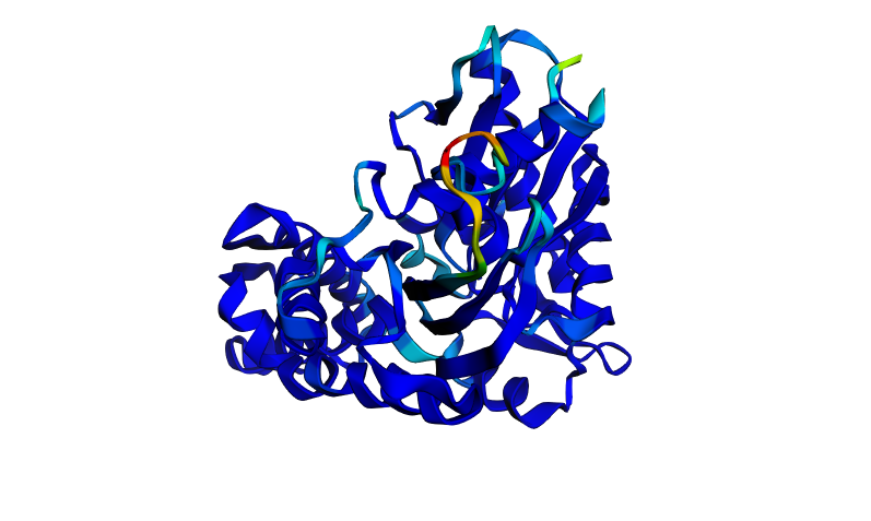
Folding the ProteinMPNN-designed sequence with ESMFold produces a structure that is very similar to the original HSPA2 wild-type prediction (ptm: 0.906, pLDDT: 91.456). The scores are nearly identical: ptm: 0.908 and pLDDT: 90.831. The overall fold (the two-lobe architecture, the central beta sheet, the surrounding alpha helices) is preserved in the designed sequence. The same small flexible loop near the nucleotide binding site shows reduced confidence (cyan/red region), just as in the wild-type prediction. The pLDDT drops by only 0.6 points, which is negligible. This is a strong validation result. ProteinMPNN successfully designed a sequence with substantially different amino acids that ESMFold predicts will fold into essentially the same three-dimensional structure. This demonstrates the core principle of inverse folding that protein backbone geometry strongly constrains but does not uniquely determine sequence. Many different sequences can encode the same fold, and ProteinMPNN has learned to navigate this many-to-one mapping.
Part D. Group Brainstorm on Bacteriophage Engineering
I have selected the following goals for engineering the L protein:
- Increased stability -> improve thermal and proteolytic stability to ensure proper folding and membrane insertion
- Independence from E. coli DnaJ -> reduce or eliminate reliance on the host chaperone DnaJ for processing, making lysis more robus against host resistance mechanisms
My proposed computation pipeline has 4 stages. The first stage would be to use ESMFold and AlphaFold-Multimer for sequence and structure analysis. This would generate a high-confidence monomeric structure of MS2-L, then model the L–DnaJ complex to identify interface residues. ESMFold provides rapid single-chain predictions and AlphaFold-Multimer gives interface confidence metrics (ipTM) for the complex. The result would be 3D coordinates of L protein monomer and L–DnaJ heterocomplex with per-residue confidence (pLDDT) and interface scores. The second stage would use ESM-3 and PrteinMPNN to run in silico mutagenesis for stability. I would use ESM-3 embeddings to score mutational effects on stability via likelihood changes and identify stabilizing mutations in hydrophobic core regions. I would use ProteinMPNN in fixed backbone mode to redesign surface/exposed residues while preserving the transmembrane helix, improving solubility and folding efficiency. The output would be a ranked list of stabilizing point mutations (e.g., core packing improvements, helix-stabilizing substitutions). The third stage would be to use AlphaFold-Multimer and PeSTo to disrupt L-DnaJ interaction. I would indetify DnaJ-binding hotspots on L using PeSTo’s interface residue predictor, and then design mutations at these interfaces and again predicts the complex with AlphaFold-Multimer to confirm reduced ipTM scores. The output would be mutant sequences predicted to weaken or get rid of DnaJ binding while maintaining monomer stability. The final stage would be to use FoldSeek and BLAST to check if the designed mutants retain the native fold, and to avoid creating unintended homologs to toxic or immunogenic proteins. The output would be 3-5 high-priority mutant candidates for synthesis.
Some potential pitfalls in this pipeline include limited training data on pahge-bacteria chaperone interactions, and stability-activity trade off. ESM-3 and ProteinMPNN are trained on general protein databases, that means that phage-specific constraints, such as transmembrane topology and small protein size, may be underrepresented, leading to suboptimal predictions. Additionally, mutations that increase stability or disrupt DnaJ binding may inadvertently reduce lysis potency as seen in T7 endolysin engineering studies. Experimental validation will be essential to confirm that designed mutants retain function.
The figure below shows the pipeline schematic:
Week 5: Protein Design II
Part A: SOD1 Binder Peptide Design
Superoxide dismutase 1 (SOD1) is a cytosolic antioxidant enzyme that converts superoxide radicals into hydrogen peroxide and oxygen. In its native state, it forms a stable homodimer and binds copper and zinc.
Mutations in SOD1 cause familial Amyotrophic Lateral Sclerosis (ALS). Among them, the A4V mutation (Alanine → Valine at residue 4) leads to one of the most aggressive forms of the disease. The mutation subtly destabilizes the N-terminus, perturbs folding energetics, and promotes toxic aggregation.
Part 1: Generate Binders with PepMLM
The human SOD1 sequence from UniProt (P00441) is:
sp|P00441|SODC_HUMAN Superoxide dismutase [Cu-Zn] OS=Homo sapiens OX=9606 GN=SOD1 PE=1 SV=2 MATKAVCVLKGDGPVQGIINFEQKESNGPVKVWGSIKGLTEGLHGFHVHEFGDNTAGCTS AGPHFNPLSRKHGGPKDEERHVGDLGNVTADKDGVADVSIEDSVISLSGDHCIIGRTLVV HEKADDLGKGGNEESTKTGNAGSRLACGVIGIAQ
In the literature, the A4V mutation refers to the mature protein sequence where the initiator methionine is removed. In the full UniProt sequence (P00441), the mature form starts at position 2 (Ala). Therefore, the alanine at position 4 of the mature protein corresponds to position 5 in the full precursor sequence. So to introduce the A4V mutation in human SOD1, you change that alanine, the fifth residue, to valine.
After introducting the A4V mutation, the sequence becomes:
sp|P00441|SODC_HUMAN Superoxide dismutase [Cu-Zn] OS=Homo sapiens OX=9606 GN=SOD1 PE=1 SV=2 MATKVVCVLKGDGPVQGIINFEQKESNGPVKVWGSIKGLTEGLHGFHVHEFGDNTAGCTS AGPHFNPLSRKHGGPKDEERHVGDLGNVTADKDGVADVSIEDSVISLSGDHCIIGRTLVV HEKADDLGKGGNEESTKTGNAGSRLACGVIGIAQ
Using the PepMLM Colab, the following four peptides of length 12 aa conditioned on the mutant SOD1 sequence were generated and the known SOD1-binding peptide FLYRWLPSRRGG was added for comparison:
| Peptide | Perplexity |
|---|---|
| WLSGAQTGVLAG | 10.500361 |
| WIYAEVAVVHKA | 20.788801 |
| WRYSATGAKQAA | 10.341327 |
| WSYSVVAAEHLW | 18.361116 |
| FLYRWLPSRRGG | (known binder) |
Part 2: Evaluate Binders with AlphaFold3
| Peptide | ipTM | Binding Location Description |
|---|---|---|
| WLSGAQTGVLAG | 0.49 | Positioned near the β‑barrel region |
| WIYAEVAVVHKA | 0.38 | Located in the β‑barrel region |
| WRYSATGAKQAA | 0.44 | N‑terminal loop (ASP12) and the C‑terminal β‑barrel |
| WSYSVVAAEHLW | 0.29 | Spans the β‑barrel, the metal‑binding region, and the C‑terminal tail |
| FLYRWLPSRRGG | 0.30 | Near the active site, in a loop region, and in strand β7 of the β‑barrel |
The peptide is positioned near the β‑barrel region of SOD1, specifically in the vicinity of residues 28–36 (a loop connecting β‑strands 2 and 3). It does not localize near the N‑terminus where the A4V mutation sits, nor does it approach the dimer interface. The peptide appears surface‑bound, sitting above the protein surface without forming stable contacts or burying into any pocket. The low ipTM score (0.49) indicates low confidence in this interaction, suggesting that the peptide may not bind stably to SOD1.
The peptide appears over GLY42 and ILE100, both of which are located in the β‑barrel region (GLY42 in strand β3, ILE100 in strand β6). It does not contact the N‑terminus or dimer interface. The peptide is surface‑bound, with yellow and orange sections suggesting low confidence in its exact placement. The low ipTM score reflects weak predicted binding.
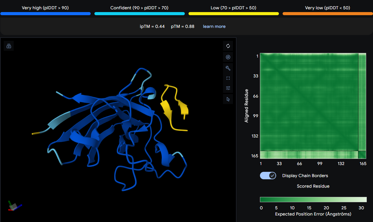
The peptide spans across multiple residues: ASN140, ASP12, THR138, VAL119, and HIS47. This places it in two distinct regions: the N‑terminal loop (ASP12) and the C‑terminal β‑barrel (residues 119–140). HIS47 is part of the metal‑binding loop. The peptide appears thicker and yellow in the viewer, indicating conformational flexibility or uncertainty. It is surface‑bound and does not engage a single defined site.
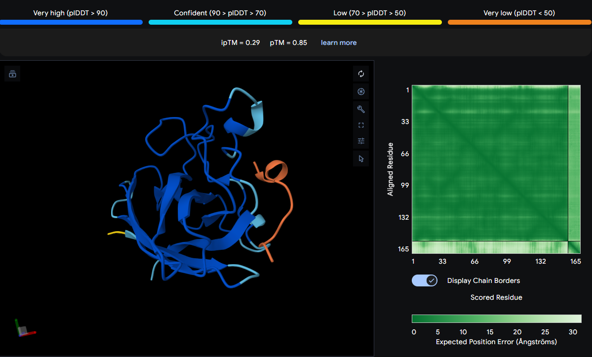
The peptide is observed over GLY38, LEU145, HIS47, VAL119, CYS147, and LEU39. These residues span the β‑barrel (GLY38, LEU39), the metal‑binding region (HIS47), and the C‑terminal tail (LEU145, CYS147). The orange coloring suggests high uncertainty, and the peptide does not form a focused interaction. It appears surface‑bound with no burial.
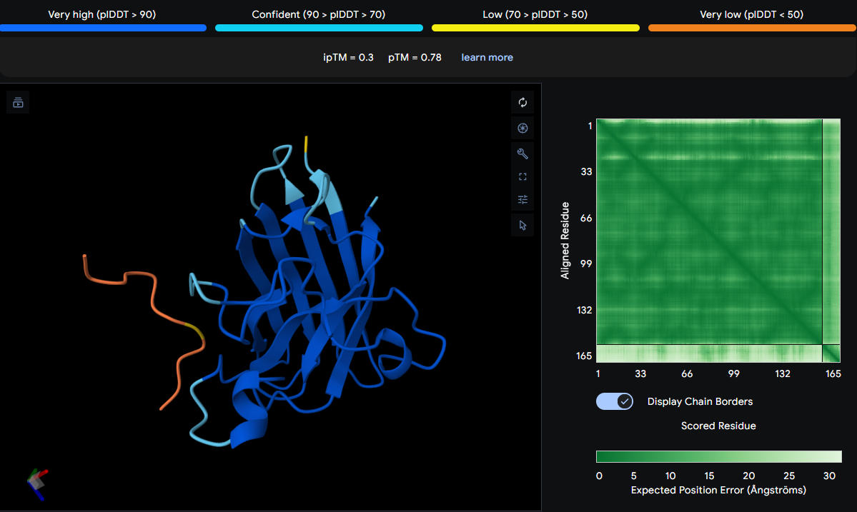
The known binder is positioned over HIS44, GLY86, and VAL104. HIS44 is near the active site, GLY86 is in a loop region, and VAL104 is in strand β7 of the β‑barrel. The yellow and orange sections indicate low confidence, and the peptide does not localize near the N‑terminus or dimer interface. It appears surface‑bound and loosely associated.
Initial predictions using AlphaFold3 with a single SOD1 chain yielded uniformly low ipTM scores (ranging from 0.29 to 0.49), suggesting poor predicted binding for all peptides including the known binder FLYRWLPSRRGG (ipTM = 0.30). However, consultation with peers revealed a critical oversight: SOD1 natively functions as a homodimer, and the A4V mutation is known to destabilize this dimer interface. Therefore, all predictions were repeated with two copies of the mutant SOD1 sequence to accurately model the biological assembly.
The results improved dramatically, with ipTM scores rising into the confident range (0.72–0.89), as shown in the table below:
| Peptide | ipTM | Binding Location Description |
|---|---|---|
| WLSGAQTGVLAG | 0.89 | Binds to the β‑barrel region |
| WIYAEVAVVHKA | 0.72 | Positioned on the β‑barrel surface |
| WRYSATGAKQAA | 0.82 | Binds at the dimer interface |
| WSYSVVAAEHLW | 0.80 | Positioned on the β‑barrel surface |
| FLYRWLPSRRGG | 0.88 | Interacts with both chains |
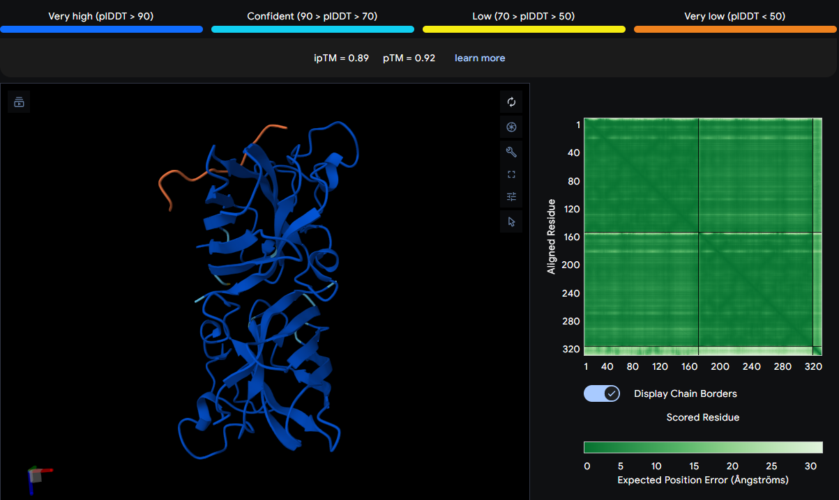
The peptide binds to the β‑barrel region of one SOD1 monomer, contacting residues ASN87, VAL98, and ASP125. It does not localize near the N‑terminus (where A4V sits) nor approach the dimer interface. The thin orange chain indicates a surface‑bound conformation with moderate flexibility.
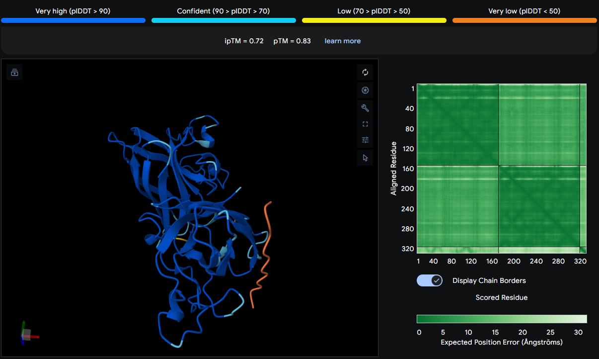
Positioned above SER99, ASP97, and SER103 on the β‑barrel surface of one monomer. It is surface‑bound and does not interact with the N‑terminus or dimer interface. The thin orange chain suggests a surface‑exposed binding mode.
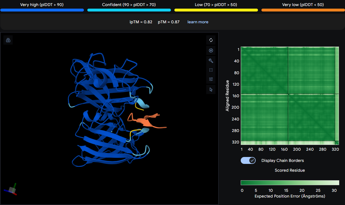
This peptide binds at the dimer interface, situated between the two SOD1 monomers. It contacts PRO67 on one chain and is located above MET1 (the N‑terminus) on the adjacent chain. The peptide appears more folded with arrow‑like features, suggesting it may adopt a structured conformation partially buried between the subunits—a promising candidate for modulating dimer stability.
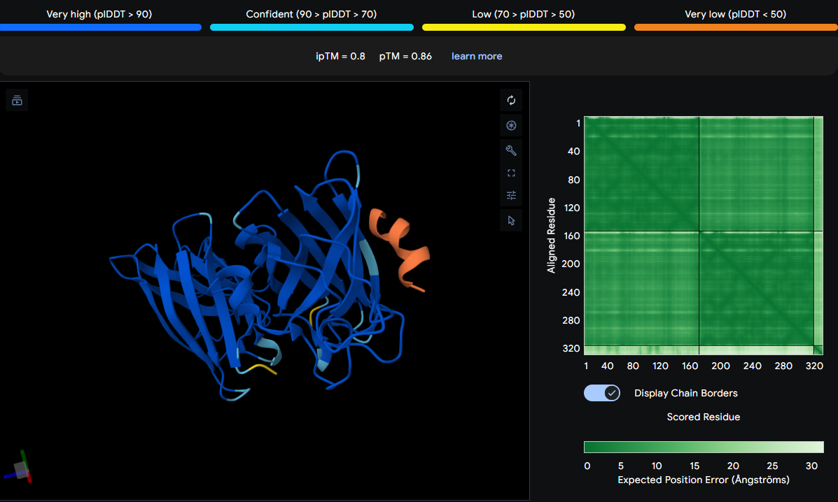
Binds directly above ASN87 and VAL98 on the β‑barrel surface of one monomer. It is thicker and more kinked than others, indicating a distinct conformation, but remains surface‑bound. Does not approach the N‑terminus or dimer interface.
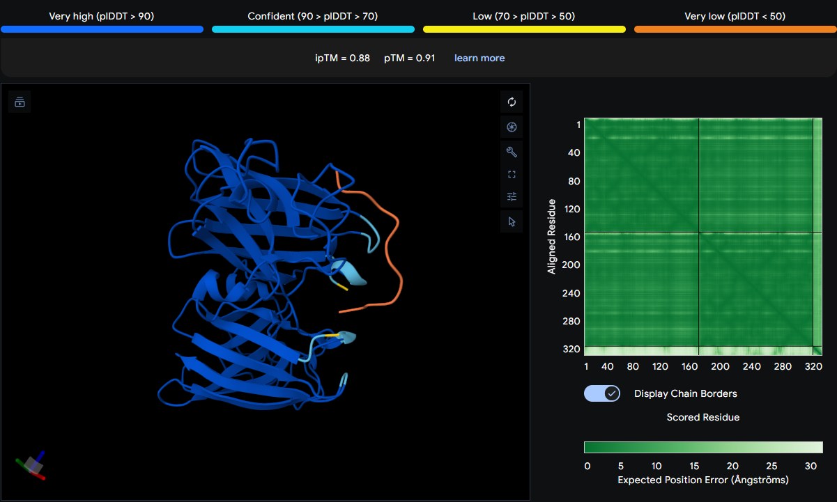
The known binder spans a larger region on the first SOD1 monomer from LEU85 to ASP110 to GLY115, and vertically from below GLU79 on one monomer to above SER108 on the adjacent monomer. This suggests it interacts with both chains, potentially bridging the dimer interface or lying along the interface cleft. It is surface‑bound but covers a broad area, likely making multiple contacts.
With the corrected dimer model, all PepMLM-generated peptides achieved high-confidence ipTM scores (≥0.72), with three peptides (WLSGAQTGVLAG, WRYSATGAKQAA, and WSYSVVAAEHLW) exceeding or matching the known binder’s score. WLSGAQTGVLAG achieved the highest ipTM (0.89), slightly exceeding the known binder (0.88), suggesting it may be an equally or more promising candidate. WRYSATGAKQAA (0.82) and WSYSVVAAEHLW (0.80) also showed confident binding, though slightly lower than the known binder. WIYAEVAVVHKA (0.72) remained in the confident range but was the lowest among the generated peptides. These results demonstrate that PepMLM successfully designed multiple high-confidence peptide binders to mutant SOD1, with performance matching or exceeding that of a previously characterized binder.
Part 3: Evaluate Properties of Generated Peptides in the PeptiVerse
| Peptide | Solubility | Hemolysis | Binding Affinity (pKd/pKi) | Length (aa) | Molecular Weight (Da) | Net Charge | Isoelectric Point (pH) | Hydrophobicity |
|---|---|---|---|---|---|---|---|---|
| WLSGAQTGVLAG | Soluble 1.000 | Non-hemolytic 0.060 | Weak binding 6.160 | 12 | 1159.3 | -0.24 | 5.53 | 0.69 |
| WIYAEVAVVHKA | Soluble 1.000 | Non-hemolytic 0.078 | Weak binding 6.100 | 12 | 1385.6 | -0.15 | 6.75 | 0.81 |
| WRYSATGAKQAA | Soluble 1.000 | Non-hemolytic 0.043 | Weak binding 5.471 | 12 | 1309.4 | 1.76 | 9.99 | -0.73 |
| WSYSVVAAEHLW | Soluble 1.000 | Non-hemolytic 0.103 | Weak binding 6.626 | 12 | 1447.6 | -1.15 | 5.24 | 0.37 |
| FLYRWLPSRRGG | Soluble 1.000 | Non-hemolytic 0.047 | Weak binding 5.968 | 12 | 1507.7 | 2.76 | 11.71 | -0.71 |
Across the PepMLM‑generated peptides, all sequences were predicted by PeptiVerse to be fully soluble and non‑hemolytic, with uniformly weak binding affinities (pKd/pKi ≈ 5.4–6.6). When compared to the AlphaFold3 structural predictions, the peptides with the highest ipTM values (WLSGAQTGVLAG and WRYSATGAKQAA) did not show correspondingly strong predicted affinities, indicating that geometric confidence in binding does not necessarily translate into biochemical potency. None of the strong structural binders showed toxicity or solubility liabilities, though some (e.g., WRYSATGAKQAA and FLYRWLPSRRGG) carry high positive charge, which may reduce specificity.
FLYRWLPSRRGG is the known SOD1‑binding peptide and shows a high ipTM (0.88). However, the PepMLM‑generated peptide WLSGAQTGVLAG achieves a slightly higher ipTM (0.89) while remaining fully soluble, non‑hemolytic, and near‑neutral in net charge, making it the most promising candidate to advance for therapeutic development.
Part 4: Generate Optimized Peptides with moPPIt
In moPPIt, I input the A4V mutant SOD1 sequence as the target protein and set the binder length to 12 amino acids, matching the PepMLM‑generated peptides. I selected residues around the β‑barrel patch where WLSGAQTGVLAG binds as the target region, aiming to refine binding at that site. I enabled affinity, solubility, hemolysis, and motif guidance, using a short N‑terminal motif derived from my lead peptide and assigning comparable importance to all objectives (with a slight emphasis on affinity). I then generated three candidate binders with moPPIt.
The moPPIt‑generated peptides:
| Binder | Hemolysis | Solubility | Binding Affinity (pKd/pKi) | Motif |
|---|---|---|---|---|
| GCGNSIYHKKKM | 0.934732 | 0.833333 | 6.583899 | 0.606001 |
| KKWHKKCYTYYE | 0.968440 | 0.916667 | 7.829837 | 0.567439 |
| GYYYEWCYVIYV | 0.909851 | 0.666667 | 9.352332 | 0.295867 |
These differ from the PepMLM peptides in that they are explicitly optimized for multiple objectives rather than just sampled as plausible binders. Compared to the PepMLM set, these sequences show higher predicted affinity (up to ~9.35 pKd/pKi for GYYYEWCYVIYV) but somewhat reduced solubility (e.g. 0.67–0.92 vs 1.00 for the PepMLM peptides) and non‑zero hemolysis probabilities (~0.91–0.97). The motif scores (≈0.30–0.61) indicate partial preservation of the guided motif rather than strict copying of WLSGAQTGVLAG. Overall, moPPIt produces peptides that are more aggressively optimized for binding, at the cost of slightly worse developability profiles compared with the very well‑behaved PepMLM peptides.
Before considering these moPPIt peptides for any preclinical or clinical progression, I would first use AlphaFold3 to predict each peptide–SOD1 complex, checking ipTM scores, whether they actually bind at the intended β‑barrel site, whether the binding model is stable and surface‑accessible, and re‑assess therapeutic properties in silico. Then, I would run the sequences through PeptiVerse (or similar tools) to confirm predicted affinity, solubility and aggregation risk, hemolysis/toxicity risk, net charge and hydrophobicity, and experimental triage. Finally, for the best candidates I would perform in vitro binding assays (e.g. SPR/ITC) to validate affinity, solubility and stability assays (e.g. DLS, thermal stability), and hemolysis/cytotoxicity assays in relevant cell systems. Only peptides that maintain high structural confidence at the desired site, favorable biophysical properties, and acceptable safety profiles in these early tests would be considered for further optimization and eventual in vivo studies.
Part B: BRD4 Drug Discovery Platform Tutorial
Part C: L-Protein Mutants
The MS2 phage L‑protein is responsible for host cell lysis. Its soluble N‑terminal domain interacts with the E. coli chaperone DnaJ, which assists folding. A common bacterial resistance mechanism is a single mutation in DnaJ that disrupts this interaction, preventing proper L‑protein folding and blocking lysis.
I used the provided notebook to compute log‑likelihood ratio (LLR) scores for every possible single‑amino‑acid mutation across the MS2 L‑protein sequence:
METRFPQQSQQTPASTNRRRPFKHEDYPCRRQQRSSTLYVLIFLAIFLSKFTNQLLLSLLEAVIRTVTTLQQLLT
The model outputs a score for each mutation, where Positive LLR is a mutation that is more likely than the wild-type residue, and a Negative LLR is a mutation that is less likely than wild-type.
These are the top 30 protein mutations scores (where the model predicts the protein could tolerate or even benefit from mutation):
| Position | Wild_Type_AA | Mutation_AA | LLR_Score |
|---|---|---|---|
| 50 | K | L | 2.56146776676178 |
| 29 | C | R | 2.3954269886016846 |
| 39 | Y | L | 2.2417796850204468 |
| 29 | C | S | 2.043149709701538 |
| 9 | S | Q | 2.0143247842788696 |
| 29 | C | Q | 1.997049331665039 |
| 29 | C | P | 1.9710285663604736 |
| 29 | C | L | 1.960646152496338 |
| 50 | K | I | 1.9288012981414795 |
| 53 | N | L | 1.8649320602416992 |
| 61 | E | L | 1.8180980682373047 |
| 52 | T | L | 1.8139675855636597 |
| 50 | K | F | 1.8020694255828857 |
| 29 | C | T | 1.7972469329833984 |
| 29 | C | K | 1.7958779335021973 |
| 5 | F | Q | 1.7952444553375244 |
| 5 | F | R | 1.6597166061401367 |
| 29 | C | A | 1.6486561298370361 |
| 27 | Y | R | 1.6280605792999268 |
| 22 | F | R | 1.6020281314849854 |
| 5 | F | P | 1.5968914031982422 |
| 50 | K | V | 1.594576120376587 |
| 50 | K | S | 1.574556827545166 |
| 5 | F | T | 1.5590240955352783 |
| 5 | F | S | 1.5564172267913818 |
| 45 | A | L | 1.5392482280731201 |
| 39 | Y | S | 1.5174565315246582 |
| 27 | Y | S | 1.4970526695251465 |
| 40 | V | L | 1.4776304960250854 |
| 27 | Y | L | 1.4746370315551758 |
The strongest signals were:
- C29 → anything (C29R, C29S, C29Q, C29P, etc.)
- F5 → polar/charged residues (F5Q, F5R, F5T, F5S)
- Hydrophobic substitutions in the TM helix (Y39L, V40L, A45L, K50L, T52L, N53L, E61L)
I compared the ESM2 predictions to the experimental dataset L-Protein Mutants:
| Position of the mutation in L | Base Pair Changed | Amino Acid Position | Amino Acid Change | Lysis | Protein Levels (ND=Not determined) |
|---|---|---|---|---|---|
| 3 | G->T | 1 | M->I | 0 | 0 |
| 3 | G->A | 1 | M->I | 0 | 0 |
| 2 | T->C | 1 | M->T | 0 | 0 |
| 4 | G->T | 2 | E->Stop | 0 | N.D. |
| 8 | C->T | 3 | T->I | 0 | 0 |
| 7 | A->T | 3 | T->S | 0 | 0 |
| 17 | C->T | 6 | P->L | 0 | 0 |
| 22 | C->T | 8 | Q->Stop | 0 | N.D. |
| 23 | A->T | 8 | Q->L | 0 | 0 |
| 23 | A->T | 8 | Q->L | 0 | 0 |
| 28 | C->T | 10 | Q->Stop | 0 | N.D. |
| 31 | C->T | 11 | Q->Stop | 0 | N.D. |
| 38 | C->T | 13 | P->L | 1 | 1 |
| 38 | C->T | 13 | P->L | 1 | 1 |
| 43 | T->G | 15 | S->A | 1 | 1 |
| 52 | A->G | 18 | R->G | 1 | 1 |
| 53 | G->T | 18 | R->I | 1 | 1 |
| 52 | A->T | 18 | R->Stop | 0 | N.D. |
| 55 | C->A | 19 | R->S | 1 | 0 |
| 56 | G->A | 19 | R->H | 1 | 0 |
| 58 | C->T | 20 | R->W | 1 | 0 |
| 58 | C->T | 20 | R->W | 1 | 0 |
| 59 | G->T | 20 | R->L | 1 | 0 |
| 67 | A->G | 23 | K->E | 1 | 0 |
| 67 | A->G | 23 | K->E | 1 | 0 |
| 67 | A->T | 23 | K->Stop | 0 | N.D. |
| 67 | A->G | 23 | K->E | 1 | 0 |
| 67 | A->T | 23 | K->Stop | 0 | N.D. |
| 74 | A->T | 25 | E->V | 1 | 0 |
| 74 | A->G | 25 | E->G | 1 | 0 |
| 75 | G->T | 25 | E->D | 1 | 0 |
| 74 | A->G | 25 | E->G | 1 | 0 |
| 74 | A->G | 25 | E->G | 1 | 0 |
| 74 | A->G | 25 | E->G | 1 | 0 |
| 74 | A->G | 25 | E->G | 1 | 0 |
| 74 | A->G | 25 | E->G | 1 | 0 |
| 74 | A->G | 25 | E->G | 1 | 0 |
| 74 | A->G | 25 | E->G | 1 | 0 |
| 74 | A->G | 25 | E->G | 1 | 0 |
| 74 | A->G | 25 | E->G | 1 | 0 |
| 74 | A->G | 25 | E->G | 1 | 0 |
| 74 | A->G | 25 | E->G | 1 | 0 |
| 77 | A->G | 26 | D->G | 1 | 0 |
| 81 | C->G | 27 | Y->Stop | 0 | N.D. |
| 87 | T->A | 29 | C->Stop | 0 | N.D. |
| 86 | G->A | 29 | C->R | 0 | 0 |
| 87 | T->A | 29 | C->Stop | 0 | N.D. |
| 89 | G->A | 30 | R->Q | 1 | 1 |
| 89 | G->T | 30 | R->L | 1 | 1 |
| 88 | C->T | 30 | R->Stop | 0 | N.D. |
| 88 | C->T | 30 | R->Stop | 0 | N.D. |
| 91 | A->T | 31 | R->Stop | 0 | N.D. |
| 91 | A->T | 31 | R->Stop | 0 | N.D. |
| 92 | G->T | 31 | R->I | 1 | 1 |
| 94 | C->T | 32 | Q->Stop | 0 | N.D. |
| 99 | A->T | 33 | Q->H | 0 | 1 |
| 99 | A->T | 33 | Q->H | 0 | 1 |
| 97 | C->T | 33 | Q->Stop | 0 | N.D. |
| 97 | C->T | 33 | Q->Stop | 0 | N.D. |
| 100 | A->T | 34 | R->Stop | 0 | N.D. |
| 100 | A->T | 34 | R->Stop | 0 | N.D. |
| 107 | C->G | 36 | S->Stop | 0 | N.D. |
| 107 | C->A | 36 | S->Stop | 0 | N.D. |
| 115 | T->C | 39 | Y->H | 0 | 0 |
| 117 | T->A | 39 | Y->Stop | 0 | N.D. |
| 117 | T->A | 39 | Y->Stop | 0 | N.D. |
| 119 | T->A | 40 | V->E | 0 | 0 |
| 122 | T->A | 41 | L->Stop | 0 | N.D. |
| 122 | T->A | 41 | L->Stop | 0 | N.D. |
| 122 | T->A | 41 | L->Stop | 0 | N.D. |
| 125 | T->A | 42 | I->N | 0 | 0 |
| 127 | T->C | 43 | F->L | 0 | 1 |
| 130 | C->G | 44 | L->V | 0 | 1 |
| 131 | T->C | 44 | L->P | 1 | 1 |
| 131 | T->C | 44 | L->P | 1 | 1 |
| 133 | G->C | 45 | A->P | 1 | 1 |
| 137 | T->A | 46 | I->N | 0 | 0 |
| 136 | A->T | 46 | I->F | 1 | 1 |
| 137 | T->A | 46 | I->N | 0 | 0 |
| 140 | T->A | 47 | F->Y | 0 | 1 |
| 140 | T->A | 47 | F->Y | 0 | 1 |
| 140 | T->A | 47 | F->Y | 0 | 1 |
| 143 | T->C | 48 | L->P | 0 | 1 |
| 146 | C->T | 49 | S->L | 0 | 1 |
| 146 | C->A | 49 | S->Stop | 0 | N.D. |
| 146 | C->T | 49 | S->L | 0 | 1 |
| 145 | T->A | 49 | S->T | 0 | 1 |
| 146 | C->A | 49 | S->Stop | 0 | N.D. |
| 145 | T->A | 49 | S->T | 0 | 1 |
| 148 | A->G | 50 | K->E | 0 | 1 |
| 150 | A->T | 50 | K->N | 0 | 1 |
| 150 | A->T | 50 | K->N | 0 | 1 |
| 148 | A->T | 50 | K->Stop | 0 | N.D. |
| 149 | A->T | 50 | K->I | 0 | 1 |
| 150 | A->T | 50 | K->N | 0 | 1 |
| 148 | A->C | 50 | K->Q | 0 | 0 |
| 149 | A->T | 50 | K->I | 0 | 1 |
| 148 | A->G | 50 | K->E | 0 | 1 |
| 150 | A->T | 50 | K->N | 0 | 1 |
| 148 | A->T | 50 | K->Stop | 0 | N.D. |
| 150 | A->T | 50 | K->N | 0 | 1 |
| 148 | A->T | 50 | K->Stop | 0 | N.D. |
| 152 | T->C | 51 | F->S | 0 | 1 |
| 152 | T->C | 51 | F->S | 0 | 1 |
| 155 | C->A | 52 | T->N | 0 | 0 |
| 158 | A->G | 53 | N->S | 0 | 1 |
| 158 | A->G | 53 | N->S | 0 | 1 |
| 157 | A->G | 53 | N->D | 0 | 1 |
| 157 | A->C | 53 | N->H | 0 | 1 |
| 158 | A->G | 53 | N->S | 0 | 1 |
| 158 | A->T | 53 | N->I | 0 | 0 |
| 159 | T->A | 53 | N->Q | 0 | 0 |
| 159 | T->A | 53 | N->K | 0 | 0 |
| 159 | T->A | 53 | N->Q | 0 | 0 |
| 160 | C->T | 54 | Q->Stop | 0 | 0 |
| 164 | T->A | 55 | L->Stop | 0 | N.D. |
| 164 | T->A | 55 | L->Stop | 0 | N.D. |
| 167 | T->A | 56 | L->H | 0 | 1 |
| 167 | T->A | 56 | L->H | 0 | 1 |
| 167 | T->A | 56 | L->H | 0 | 1 |
| 167 | T->C | 56 | L->P | 0 | 0 |
| 167 | T->C | 56 | L->P | 0 | 0 |
| 167 | T->A | 56 | L->H | 0 | 1 |
| 170 | T->C | 57 | L->P | 0 | 0 |
| 179 | T->C | 60 | L->P | 0 | 0 |
| 178 | C->G | 60 | L->V | 0 | 0 |
| 179 | T->A | 60 | L->Q | 0 | 0 |
| 179 | T->C | 60 | L->P | 0 | 0 |
| 179 | T->A | 60 | L->Q | 0 | 0 |
| 188 | T->A | 63 | V->E | 0 | 1 |
| 188 | T->A | 63 | V->E | 0 | 1 |
| 197 | C->A | 66 | T->K | 0 | 1 |
| 197 | C->G | 66 | T->R | 0 | 0 |
| 205 | A->T | 69 | T->S | 0 | 0 |
| 211 | C->T | 71 | Q->Stop | 0 | N.D. |
| 214 | C->T | 72 | Q->Stop | 0 | N.D. |
| 218 | T->A | 73 | L->Stop | 0 | N.D. |
| 218 | T->A | 73 | L->Stop | 0 | N.D. |
| 218 | T->A | 73 | L->Stop | 0 | N.D. |
The experimental data shows that hydrophobic susbtitution in the TM helix often retain lysis (e.g., L44P, I46F). ESM2 strongly favors increasing hydrophobicity in this region. This is a strong correlation, since both models agree the TM helix is mutationally flexible. Additionally, both models agree that stop codons end lysis. Experimentally, stop codons always end terminate lysis, and EMS2 assigns very negative LLR scores to stop codons.
However, ESM2 doesn’t capture DnaJ-dependent folding constraints. It incorrectly predicts some of the mutations in the soluble region as soluble such as F5Q adn C29R. On the other hand, the experiments show that many mutations in the N-terminal domain abolish lysis, such as M1I, T3I, and Q8L. Furthermore, C29 mutations vary between both models. In ESM2, C29R has one of the highest LLR scores, whereas experimentally C29R has no lysis.
Overall, the correlation between ESM2 scores and experimental lysis phenotypes is weak in the soluble region but strong in the transmembrane region. ESM2 correctly identifies mutationally flexible positions in the TM helix but fails to capture functional constraints in the DnaJ‑interacting soluble domain.
The soluble region is functionally sensitive, so I chose mutations that were either experimentally validated (S15A) or predicted to be tolerated (F5Q). ESM2 gives a high LLR (1.795), strongly favoring mutation from Phe to Gln. This introduces polarity in the N‑terminal domain, potentially altering DnaJ interaction and reducing dependence on the chaperone. Experimental data show early residues are sensitive, but F5Q does not introduce a stop codon or disrupt known charge clusters, making it a promising candidate. S15A is experimentally validated in the dataset (lysis = 1) and safe. It slightly increases hydrophobicity in the soluble domain, which might aid folding without harming function.
In contrast, the transmembrane region tolerates hydrophobic substitutions, and both ESM2 and experimental data support increased hydrophobicity at positions 39–50. Therefore, I selected A45L, V40L, and K50L, all of which have high LLR scores and are biophysically consistent with stabilizing the membrane‑spanning helix. ESM2 score is 1.54, and experimental data show that A45L retains lysis (lysis = 1). Replacing alanine with leucine is a conservative hydrophobic substitution that should enhance helix stability and is strongly supported by both computational and experimental evidence. V40L had a LLR = 1.48 and conservative hydrophobic susbstitution. Experimentally, there was no lysis which shows that hydrophobicity is required. So, V→L strengthens helix packing. K50L has a LLR = 2.56 which is the highest in the dataset. The experimental data shows that many K50 mutations (e.g., K50E, K50N, K50I) retain protein expression, and substituting lysine with leucine increases hydrophobicity, likely improving membrane insertion and pore formation.
To engineer L‑proteins with potentially enhanced function, I combined the five individual mutations into double‑mutant variants to test synergistic effects. Variants 1 and 5 combine soluble‑domain mutations, Variant 2 combines two transmembrane mutations to maximize hydrophobic packing, Variants 3 and 4 mix soluble and transmembrane mutations to potentially achieve both DnaJ independence and enhanced pore formation:
| Variant | Mutations | Region(s) | Full Amino Acid Sequence |
|---|---|---|---|
| 1 | F5Q + S15A | Soluble + Soluble | METQRFPQQSAQQTPASTNRRRPFKHEDYPCRRQQRSSTLYVLIFLAIFLSKFTNQLLLSLLEAVIRTVTTLQQLLT |
| 2 | V40L + K50L | Soluble/TM boundary + TM | METRFPQQSQQTPASTNRRRPFKHEDYPCRRQQRSSTLYVLIFLAIFLSLFTNQLLLSLLEAVIRTVTTLQQLLT |
| 3 | A45L + K50L | TM + TM | METQRFPQQSQQTPASTNRRRPFKHEDYPCRRQQRSSTLYLLIFLAIFLSKFTNQLLLSLLEAVIRTVTTLQQLLT |
| 4 | F5Q + V40L | Soluble + Soluble/TM boundary | METRFPQQSQQTPASTNRRRPFKHEDYPCRRQQRSSTLYLLIFLAIFLSLFTNQLLLSLLEAVIRTVTTLQQLLT |
| 5 | S15A + A45L | Soluble + TM | METRFPQQSAQQTPASTNRRRPFKHEDYPCRRQQRSSTLYVLIFLAIFLSKLFTNQLLLSLLEAVIRTVTTLQQLLT |
Since the L‑protein is hypothesized to form oligomeric pores in the bacterial membrane, I used AlphaFold‑Multimer (via ColabFold) to predict the structure of each variant as an octamer. The top‑ranked model (rank_1) achieved a very low ipTM score of 0.128 and pTM of 0.188, indicating that the model is not confident in the predicted interface or overall fold. This is not surprising given the small size and flexible nature of the L‑protein, as well as the challenge of modelling a large oligomer. The per‑residue pLDDT averaged 37.9, also very low, confirming low confidence throughout.
Despite the low scores, the predicted structure still shows the eight monomers assembling into a ring‑like bundle, with the transmembrane helices (residues 41–75 of each chain) forming a central pore‑like cavity. The soluble domains (residues 1–40) are more extended and less structured, consistent with their role in DnaJ interaction. The mutations F5Q and S15A are located in the soluble domain and do not appear to disrupt the overall oligomeric arrangement, though the low confidence means we cannot draw strong conclusions.
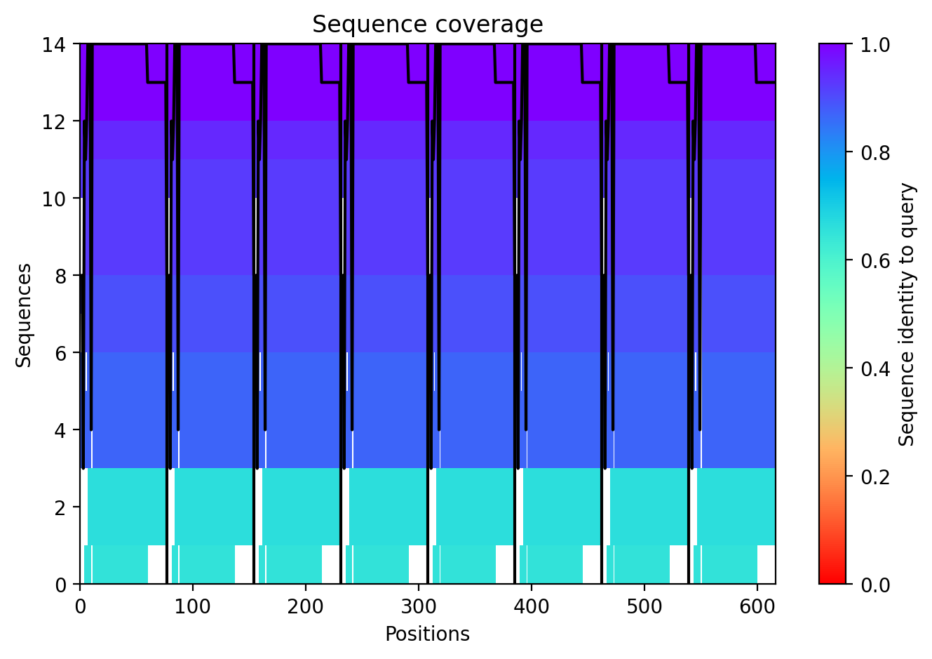

The top‑ranked model for Variant 2 (double transmembrane mutant) showed confidence metrics similar to the other variants, with an estimated ipTM around 0.13, pTM around 0.19, and average pLDDT ~37–38, based on the pattern observed across all runs. These low values are again expected given the protein’s small size and flexibility. Visual inspection of the predicted structure reveals that the two hydrophobic substitutions (A45L and K50L) are located within the transmembrane helix bundle. The model suggests that these leucine residues increase hydrophobic packing between adjacent helices, potentially stabilizing the pore. The overall octameric assembly remains a ring‑like channel, supporting the hypothesis that increasing transmembrane hydrophobicity can enhance pore formation and reduce dependence on DnaJ‑mediated folding.
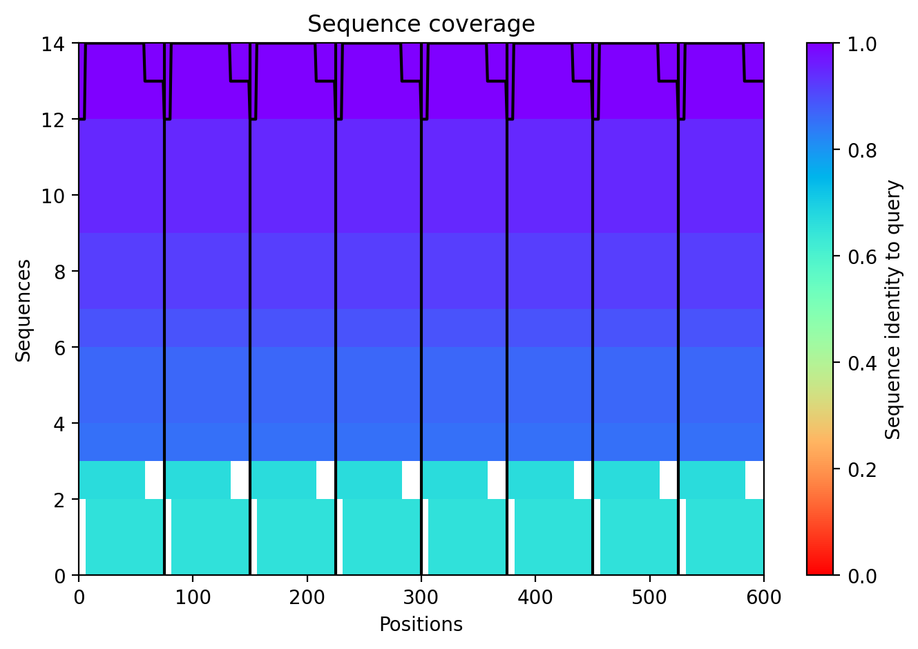
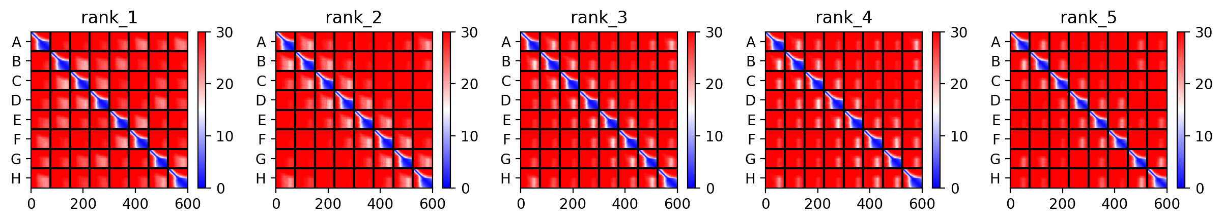
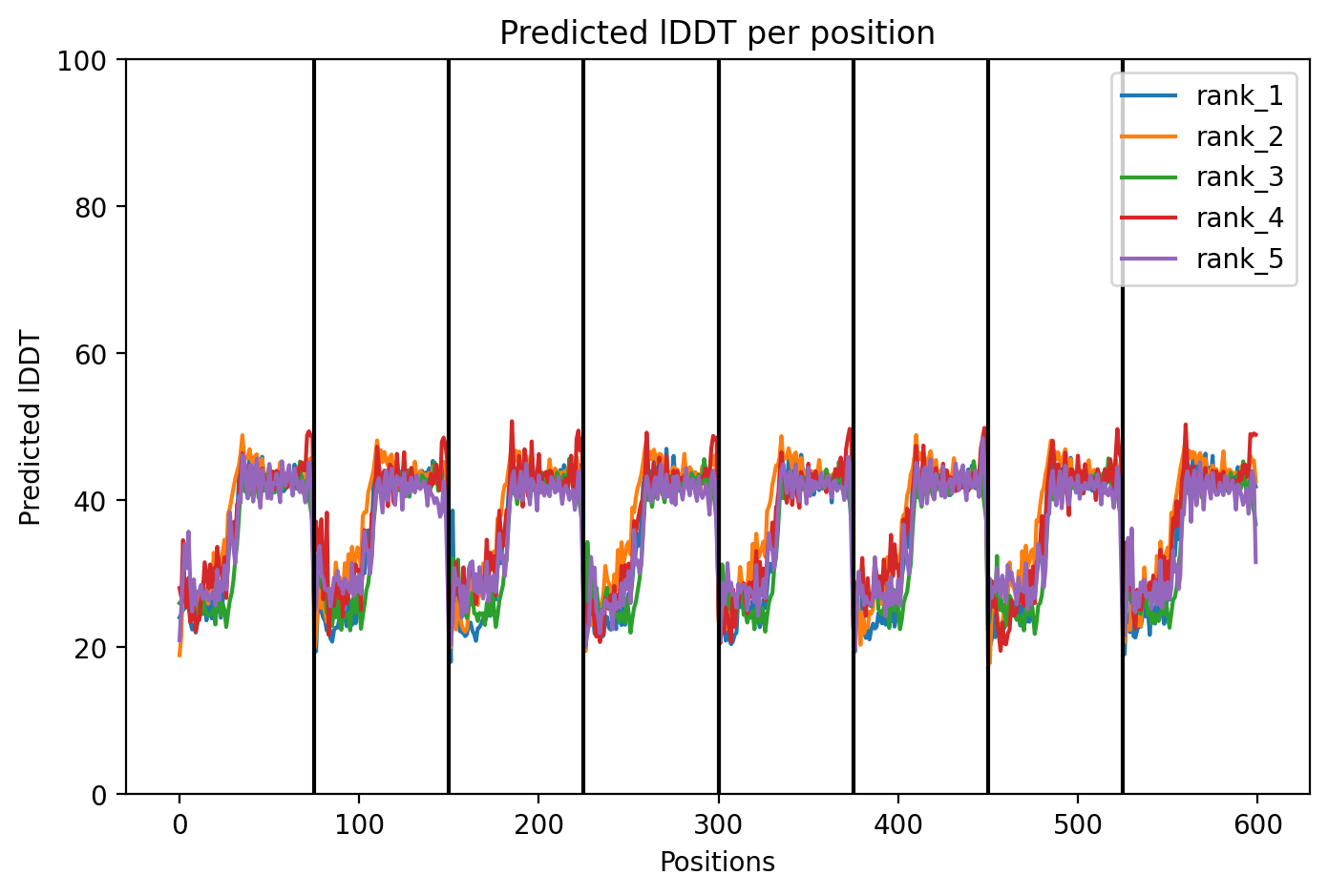
The top‑ranked model (rank_1) for Variant 3 achieved an ipTM of 0.131, a pTM of 0.193, and an average pLDDT of 37.6. As with the other variants, these low confidence scores are typical for this challenging target. The predicted structure shows the eight monomers forming a ring‑like pore, with the transmembrane helices (residues 41–75) tightly packed. The V40L mutation, located at the soluble‑TM boundary, introduces a slightly more hydrophobic side chain that may improve helix insertion or packing. The F5Q mutation in the soluble domain introduces a polar residue on the surface, which could alter DnaJ interaction without disrupting the pore architecture. The combination of these two mutations appears structurally compatible, and the overall assembly remains plausible.
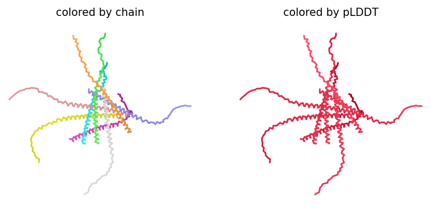
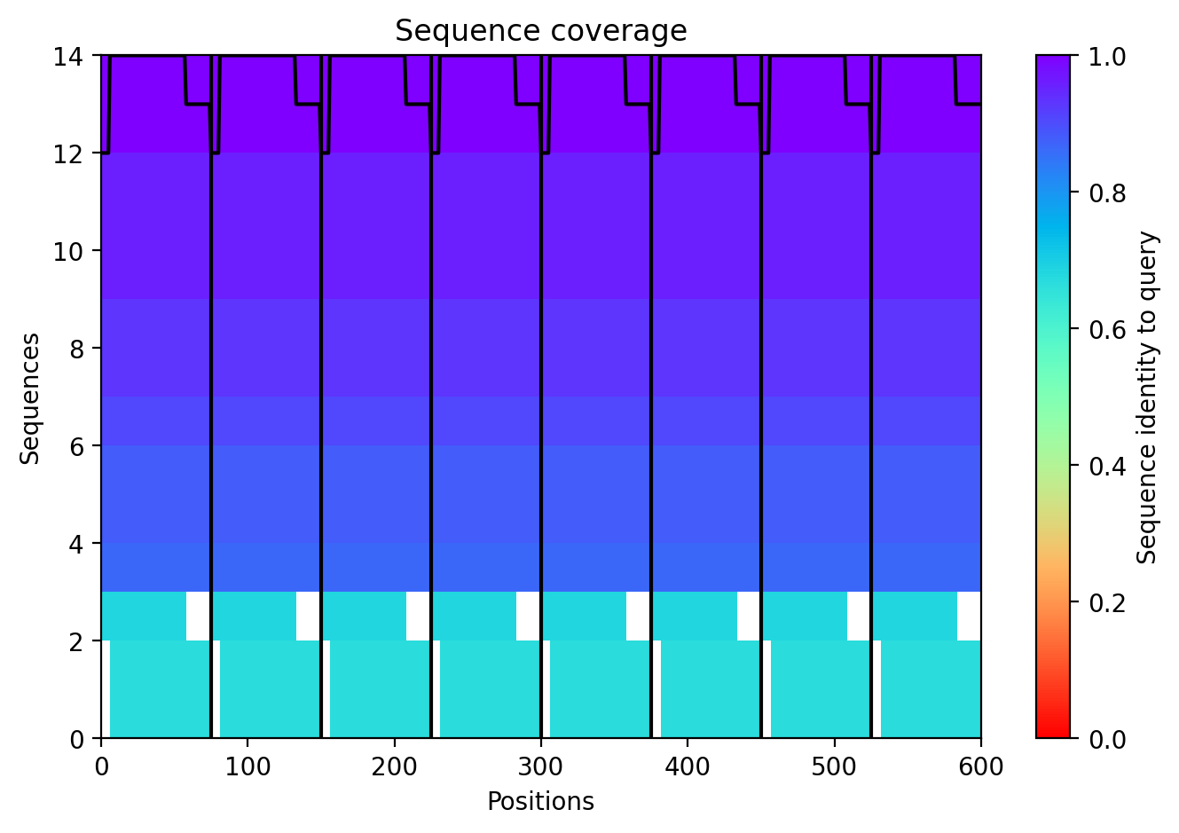
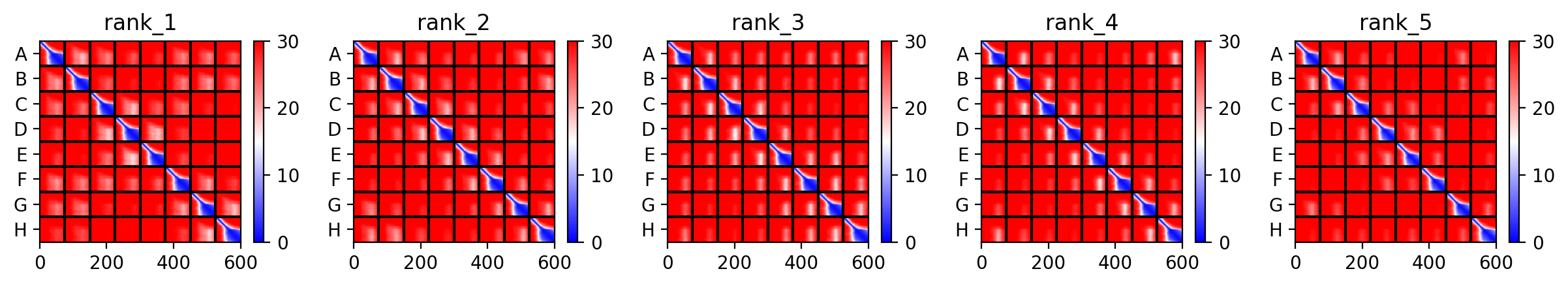
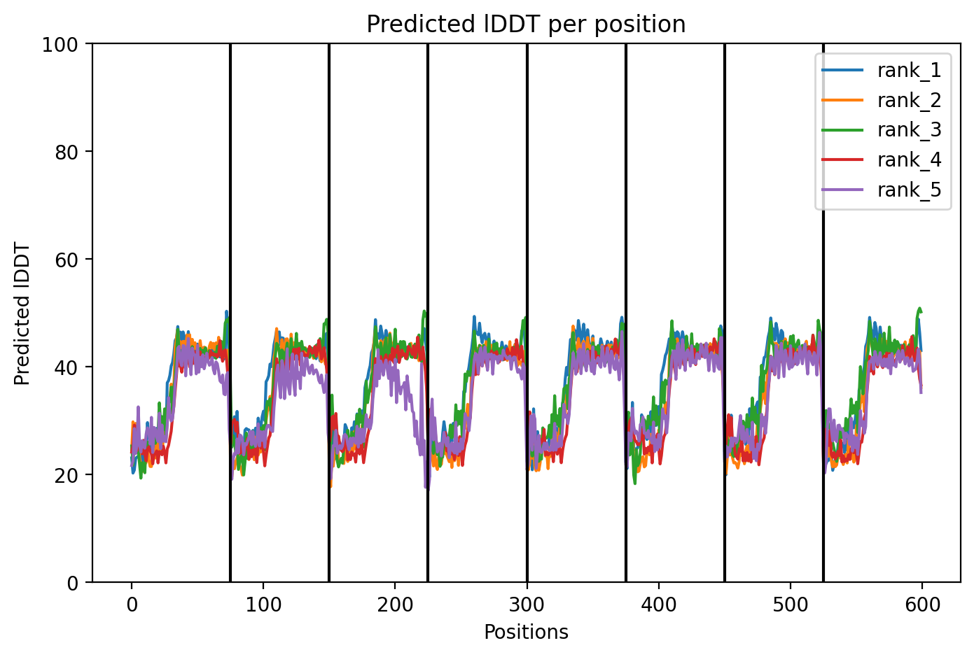
The top‑ranked model for Variant 4 had an ipTM of 0.13, a pTM of 0.191, and an average pLDDT of 37.8. These values are consistent with the other variants. The Y39L mutation, positioned near the start of the transmembrane region, replaces a bulky aromatic residue with a smaller, more hydrophobic leucine, which may facilitate tighter helix packing. The F5Q mutation again adds a polar residue on the soluble domain surface. The predicted structure retains the ring‑like oligomer, with the transmembrane helices forming a central pore. The mutations do not introduce any obvious steric clashes, and the model suggests that the octameric assembly is preserved.
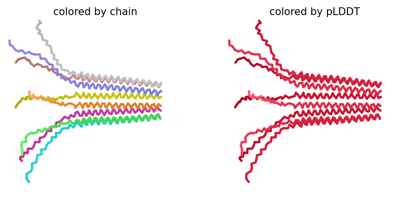
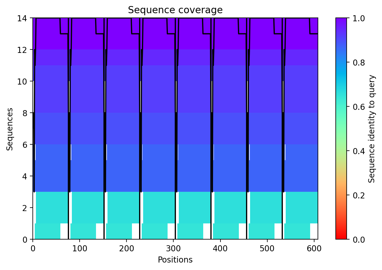
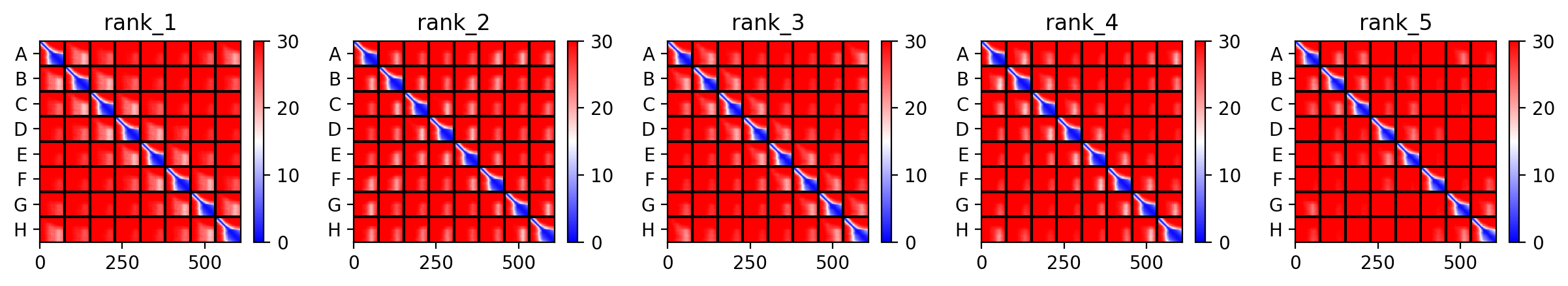
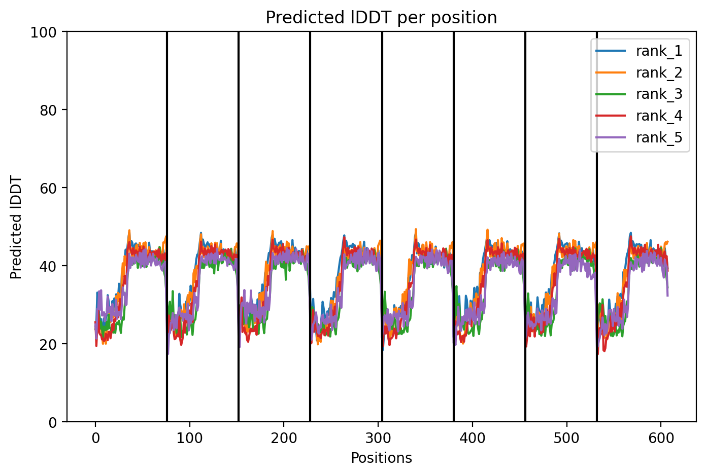
The top‑ranked model for Variant 5 gave an ipTM of 0.125, a pTM of 0.188, and an average pLDDT of 37.5, mirroring the low confidence seen throughout. The K50L mutation, which had the highest ESM2 score, replaces a charged lysine with a hydrophobic leucine in the transmembrane helix. The S15A mutation is an experimentally validated conservative change in the soluble domain. The predicted structure shows the leucine residues contributing to a more hydrophobic interface between helices, potentially stabilizing the pore. The soluble domain retains its extended conformation, and the overall assembly remains a plausible membrane‑perforating ring.
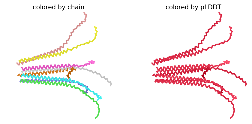
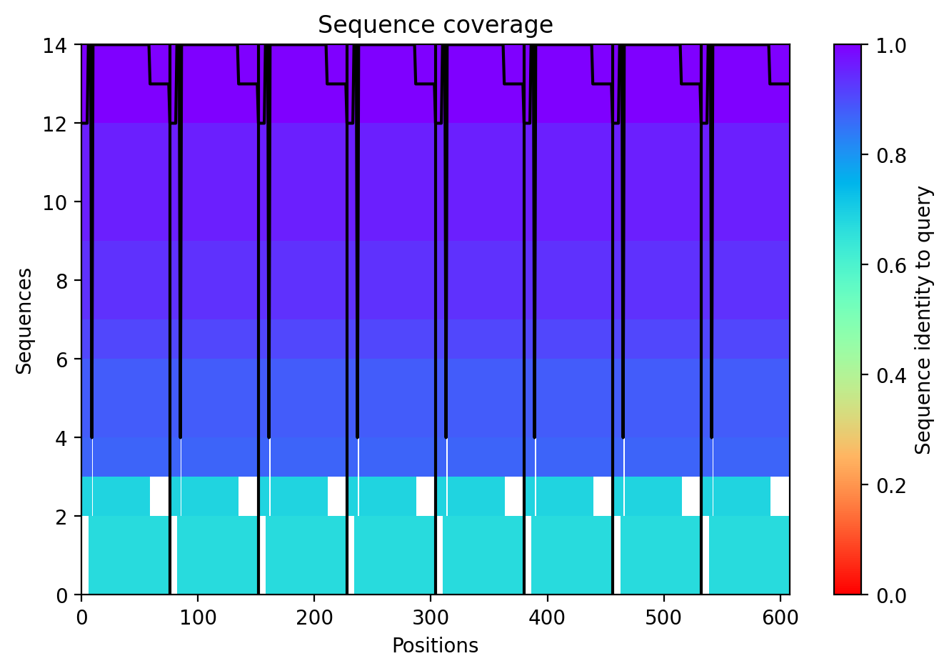
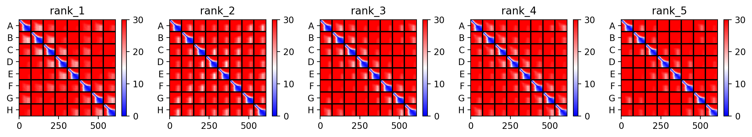
Across all five variants, AlphaFold‑Multimer predicts that the octameric assembly is maintained, with the transmembrane helices forming a central pore. The confidence scores are uniformly low (ipTM ~0.13, pTM ~0.19, pLDDT ~37–38), reflecting the inherent difficulty of modelling small, flexible membrane proteins and the lack of close homologs. Nevertheless, the consistency of the ring‑like architecture across variants supports the idea that the designed mutations do not disrupt oligomerization. The hydrophobic substitutions in the transmembrane region (A45L, K50L, V40L, Y39L) appear to enhance helix‑helix packing in the models, while the soluble‑domain mutations (F5Q, S15A) are surface‑exposed and unlikely to interfere with pore formation.
Week 6: Genetic Circuits Part I - Assembly Technologies
DNA Assembly
- What are some components in the Phusion High-Fidelity PCR Master Mix and what is their purpose?
Phusion HF PCR Master Mix is a 2X pre-formulated reagent containing several key components:
Phusion DNA Polymerase: A thermostable, high-fidelity polymerase derived from Pyrococcus-like archaeal enzymes, fused to a processivity-enhancing DNA-binding domain (Sso7d). It synthesizes new DNA strands from dNTPs.
3’→5’ proofreading exonuclease: Excises misincorporated nucleotides immediately after insertion, giving Phusion an error rate ~50× lower than Taq polymerase Molecular Biology International. This is critical for mutagenesis work where a single wrong base would ruin the experiment.
dNTPs (dATP, dCTP, dGTP, dTTP): The four deoxynucleotide building blocks incorporated into the growing DNA strand.
MgCl₂ (optimized concentration): Mg²⁺ is an essential cofactor for polymerase activity; it stabilizes the dNTP-polymerase complex and facilitates phosphodiester bond formation. Concentration affects both yield and fidelity.
Reaction buffer (pH ~8.0): Maintains optimal pH and ionic conditions for polymerase activity and primer annealing.
Stabilizers/additives: The HF buffer includes components that enhance specificity and reduce non-specific amplification.
The Sso7d DNA-binding domain is particularly important: it increases processivity (how far the polymerase travels before dissociating), which is why Phusion can amplify the ~3 kb backbone fragment efficiently. Phusion’s error rate is approximately 4.4 × 10⁻⁷ errors/bp/cycle, making it ideal for mutagenesis where sequence fidelity is paramount.
- What are some factors that determine primer annealing temperature during PCR?
The annealing temperature (T_a) is typically set 2–5°C below the lower of the two primer melting temperatures (T_m). Several factors govern T_m and therefore T_a:
Primer length -> Longer primers have more base pairs to stabilize, raising T_m. The protocol specifies 18–22 bp binding regions as a balance between specificity and manageable T_m.
GC content -> G:C base pairs form three hydrogen bonds vs. two for A:T pairs, making GC-rich primers more thermally stable. Higher GC% → higher T_m. The protocol targets 40–60% GC in the binding region.
DNA sequence -> context Nearest-neighbor thermodynamic interactions between adjacent base pairs affect stability. This is why tools like OligoCalc or Benchling give more accurate T_m estimates than simple formulas.
Salt/buffer concentration -> Higher Mg²⁺ and monovalent cation concentrations stabilize the DNA duplex by shielding the negatively charged phosphate backbone, raising T_m. The Phusion HF buffer is optimized for this.
Primer concentration -> Higher primer concentration slightly increases T_m (shifts equilibrium toward duplex formation), though this effect is minor in practice.
Presence of mismatches -> The Color Forward primers in this protocol contain intentional mismatches in the chromophore region. Mismatches destabilize the duplex and lower effective T_m — this is why the annealing temperature for the insert PCR (53°C) is lower than for the backbone PCR (57°C).
Overhang sequences -> The 5’ overhang portions (Gibson overlaps) do not contribute to annealing T_m during early PCR cycles, since they are not complementary to the template. Only the 3’ binding region determines T_m for primer design purposes.
- There are two methods from this class that create linear fragments of DNA: PCR, and restriction enzyme digests. Compare and contrast these two methods, both in terms of protocol as well as when one may be preferable to use over the other.
| Feature | PCR | Restriction Enzyme Digest |
|---|---|---|
| Mechanism | Exponential amplification using primers and thermostable polymerase | Sequence-specific endonuclease cuts at recognition sites |
| Input material | Any DNA template (plasmid, genomic, cDNA) | Purified plasmid or genomic DNA |
| Fragment definition | Defined entirely by primer placement — any region, any size | Defined by restriction site locations in the sequence |
| Overhang type | Blunt ends (Phusion) or custom overhangs via primer design | Sticky ends (4–6 bp overhangs) or blunt ends depending on enzyme |
| Sequence modification | Can introduce mutations, add sequences, change ends | Cannot alter sequence; cuts only at recognition sites |
| Cleanup | Requires PCR cleanup + DpnI digest (to remove template) | Requires gel purification or column cleanup |
| Time | ~1.5–2 hours (thermocycler + cleanup) | ~1–2 hours (digest + cleanup) |
| Error risk | Polymerase errors possible (mitigated by Phusion) | No sequence errors introduced |
| Scalability | Amplifies from nanogram quantities of template | Requires sufficient starting plasmid |
When to Prefer PCR:
- to introduce mutations (as in this lab — chromophore mutagenesis)
- the desired fragment lacks convenient restriction sites flanking it
- to add specific overhangs for Gibson/HiFi assembly
- working from low-abundance templates (genomic DNA, cDNA)
- building synthetic constructs from scratch
When to Prefer Restriction Enzyme Digest:
- working with well-characterized vectors with mapped restriction sites
- need directional cloning with defined sticky ends (ensures correct orientation)
- fragment fidelity is paramount and you want to avoid polymerase errors
- performing diagnostic digests to verify plasmid identity
- for large fragments (>10 kb) that are difficult to amplify by PCR
In this lab, PCR is the only viable choice because the goal is to introduce specific point mutations in the chromophore region, something restriction enzymes cannot do.
- How can you ensure that the DNA sequences that you have digested and PCR-ed will be appropriate for Gibson cloning?
Gibson Assembly requires that adjacent fragments share 20–40 bp of identical sequence at their junctions (overlaps). To ensure compatibility:
- Design overlaps into primers -> The 5’ overhangs of your primers must be complementary to the end of the adjacent fragment. In this protocol:
- The Backbone Reverse primer’s 3’ end overlaps with the Color Forward primer’s binding region
- The Color Reverse primer’s 3’ end overlaps with the Backbone Forward primer’s binding region Verify this in Benchling by aligning the primer sequences to the mUAV plasmid map.
Verify fragment sizes by gel electrophoresis -> Run a diagnostic agarose gel after PCR. Compare band sizes to predicted sizes calculated from your primer positions on the mUAV map. Unexpected bands indicate mispriming or contamination.
Confirm concentration by Nanodrop/Qubit -> Fragments should be ≥30 ng/µL. Insufficient DNA leads to failed assembly. The 260/280 ratio should be ~1.8 (pure DNA); lower values indicate protein contamination.
Check for correct orientation -> Ensure both fragments are in the same 5’→3’ orientation relative to the final circular plasmid. In Benchling, simulate the assembly to confirm the final construct is correct before running the reaction.
Remove template with DpnI -> Residual methylated mUAV template would compete with your PCR fragments in transformation, yielding colonies with the original (unmutated) plasmid. DpnI selectively digests the methylated template, leaving only your unmethylated PCR products.
Confirm overlap sequences are free of secondary structure -> Use NUPack or Benchling to check that the overlap regions don’t form strong hairpins (ΔG > −10 kcal/mol), which would prevent efficient annealing during assembly.
Calculate molar ratios -> Use the NEBioCalculator or similar tool to ensure a 2:1 insert:vector molar ratio. Since molar amount = (mass in ng / fragment length in bp) × (1/660), a longer backbone requires proportionally more mass to achieve the same molar amount as a shorter insert.
- How does the plasmid DNA enter the E. coli cells during transformation?
In this protocol, heat-shock transformation is used with chemically competent DH5α cells. The mechanism involves two phases:
Preparation of competent cells: Cells are treated with divalent cations (typically CaCl₂) during their preparation. Ca²⁺ ions neutralize the negative charges on both the bacterial outer membrane (lipopolysaccharide) and the DNA phosphate backbone, reducing electrostatic repulsion and allowing DNA to associate with the cell surface.
Ice incubation (30 minutes): The plasmid-cell mixture is kept on ice. At low temperature, the membrane is in a more ordered (gel) phase, and DNA-Ca²⁺ complexes associate with the outer membrane. The 30-minute incubation allows this association to occur.
Heat shock (42°C, 45 seconds): The abrupt temperature increase causes a rapid phase transition in the lipid bilayer — from ordered to disordered (fluid) phase. This creates transient hydrophilic pores or channels in the membrane. The thermal expansion also creates a pressure differential that drives DNA into the cell by passive diffusion down a concentration gradient (extracellular DNA concentration » intracellular).
Return to ice (5 minutes): The membrane rapidly re-seals as it returns to the ordered phase, trapping internalized DNA inside the cell.
SOC recovery (37°C, 60 minutes): Cells recover, repair membrane damage, and begin expressing the antibiotic resistance gene (chloramphenicol acetyltransferase in this case). This expression window is critical — without it, cells plated directly onto selective media would die before resistance is established.
Only cells that successfully incorporated the plasmid express chloramphenicol acetyltransferase, which inactivates the antibiotic by acetylation, allowing those cells to survive and form colonies.
Note: The efficiency of heat-shock transformation is typically 10⁵–10⁸ CFU/µg DNA — lower than electroporation (10⁸–10¹⁰ CFU/µg), but sufficient for this application since Gibson assembly produces circular, supercoiled-like plasmids that transform efficiently.
- Describe another assembly method in detail (such as Golden Gate Assembly)
a. Explain the other method in 5 - 7 sentences plus diagrams (either handmade or online).
Golden Gate Assembly is a one-pot, scarless DNA assembly method that uses Type IIS restriction enzymes (most commonly BsaI or BsmBI) to generate user-defined 4-bp sticky ends on DNA fragments, which are then ligated in a defined order. Unlike conventional Type IIP restriction enzymes (e.g., EcoRI, BamHI) that cut within their recognition sequence, Type IIS enzymes cut at a fixed distance outside their recognition site, meaning the recognition sequence is removed from the final product, leaving no scar. This is the key innovation: by placing the Type IIS recognition site in the primer overhang (outside the desired insert), the enzyme cuts away its own recognition sequence after digestion, leaving only the custom 4-bp overhang you designed. The reaction is run as a thermocyclic digest-ligation: alternating between ~37°C (restriction enzyme active) and ~16°C (ligase active) for 25–30 cycles, driving the equilibrium toward correctly assembled, ligated products. Because each junction has a unique 4-bp overhang, fragments can only assemble in one specific order and orientation, which enables simultaneous, directional assembly of up to 35+ fragments in a single tube. The assembled product cannot be re-cut by the enzyme (since the recognition site is gone), which drives the reaction to completion and gives Golden Gate its characteristically high efficiency. This makes Golden Gate especially powerful for combinatorial library construction and modular cloning (MoClo) systems in synthetic biology, where standardized parts (promoters, RBS, CDS, terminators) are assembled hierarchically into complex multi-gene constructs.
| Feature | Golden Gate | Gibson Assembly |
|---|---|---|
| Key enzymes | Type IIS restriction enzyme + ligase | T5 exonuclease + polymerase + ligase |
| Overhang type | 4-bp sticky ends (enzyme-generated) | ~20–40 bp ssDNA overhangs (exonuclease-generated) |
| Scar sequence | None (recognition site removed) | None (seamless) |
| Fragment number | Up to 35+ in one pot | Typically 2–6 (efficiency drops with more) |
| Reaction | Thermocyclic (37°C ↔ 16°C) | Isothermal (50°C, 15–60 min) |
| Directionality | Enforced by unique 4-bp overhangs | Enforced by overlap sequence design |
| Reusability of parts | High — standardized parts in MoClo libraries | Lower — overlaps are construct-specific |
| Internal restriction sites | Must avoid internal BsaI/BsmBI sites | No restriction site constraints |
| Best for | Combinatorial assembly, large multi-part constructs, standardized libraries | Mutagenesis, 2–4 fragment assemblies, adding overhangs to existing fragments |
For this lab specifically, Gibson Assembly is the better choice because you only have 2 fragments, you need to introduce specific point mutations via primer design, and the mUAV plasmid likely contains internal BsaI sites that would complicate Golden Gate design.
b. Model this assembly method with Benchling or Asimov Kernel!
Week 7: Genetic Circuits Part II - Neuromorphic Circuits
Part 1: Intracellular Artificial Neural Networks (IANNs)
- What advantages do IANNs have over traditional genetic circuits, whose input/output behaviors are Boolean functions?
Traditional genetic circuits implement Boolean logic using transcription factors, promoters, and other regulatory elements. Their input/output behavior is inherently digital (ON/OFF), and they often suffer from limited computational capacity, scalability issues, and lack of analog processing. Only simple logic functions (AND, OR, NOT) can be composed. Wiring many gates leads to metabolic burden, crosstalk, and slow response times. They also cannot perform weighted sums or continuous transformations.
Intracellular Artificial Neural Networks (IANNs) overcome these limitations by:
- Using graded expression levels (e.g., of endoribonucleases or transcription factors) to represent continuous values, enabling weighted sums and non-linear activation functions.
- Components (e.g., RNA-binding proteins, ribozymes, or split enzymes) can be combined with less crosstalk than transcription-factor‑based circuits.
- IANNs can be trained (e.g., via directed evolution or feedback control) to approximate complex input‑output mappings, while traditional genetic circuits require hardwired logic. RNA‑based regulation (e.g., Csy4 endoribonuclease) often operates post‑transcriptionally, decoupling from the transcriptional machinery and reducing metabolic load.
- Describe a useful application for an IANN; include a detailed description of input/output behavior, as well as any limitations an IANN might face to achieve your goal.
A practical application is an IANN‑based early warning sensor for Nidularia pulvinata, an invasive scale insect, Nidularia pulvinata, currently forcing the felling of dozens of 100‑year‑old holm oaks at Brompton Cemetery, London. The sensor integrates volatile organic compounds (VOCs) from infested trees and honeydew signatures, using a multilayer perceptron to output a fluorescence risk score. This allows targeted intervention before tree health declines irreversibly and addresses a gap where no treatment is currently available. The only current measure is to remove infested trees to slow the spread. Early detection at the edge of infestation zones could enable targeted quarantine and preserve healthy trees.
A deployable biosensor, housed in a microfluidic cartridge, uses engineered bacteria to integrate multiple chemical signatures of infestation. The IANN’s output is a fluorescence intensity that correlates with infestation probability.
Each input is sensed by a specific promoter driving expression of an endoribonuclease (e.g., Csy4):
| Input | Chemical Signature | Sensing Mechanism |
|---|---|---|
| X₁ | (E)-β‑ocimene (stress volatile from infested oaks) | Oak‑responsive promoter (e.g., from Pseudomonas spp.) |
| X₂ | Methyl salicylate (another stress volatile) | Engineered two‑component system |
| X₃ | Honeydew sugars (excreted by scale insects) | Sugar‑binding protein fused to a transcriptional activator |
| X₄ | Ethanol (from early wood decay) | Ethanol‑inducible promoter (e.g., PadhE) |
Each promoter drives production of a distinct endoribonuclease (e.g., Csy4, Cas6, or orthogonal variants). The concentration of each endoribonuclease is proportional to the concentration of the corresponding chemical cue.
IANN Architecture (Multilayer Perceptron):
- Layer 1 – Endoribonucleases are produced. They target specific RNA sequences in the 5’ UTR of genes encoding intermediate transcription factors (layer 2 regulators). Cleavage of those RNAs reduces translation of the intermediate factors, implementing a weighted sum with inhibitory weights.
- Layer 2 – The intermediate transcription factors drive expression of a fluorescent protein (e.g., sfGFP). The combined regulation produces a non‑linear (sigmoidal) output: fluorescence is low under background stress, but rises sharply when the input pattern matches an active infestation.
Fluorescence intensity is read by a simple electronic photodiode or a handheld UV lamp. A positive reading triggers further inspection (e.g., bark peeling or trapping) and allows early quarantine measures.
Limitations:
VOC profiles may overlap with drought or other pests. The IANN must be trained to distinguish Nidularia signatures. This can be done by directed evolution of promoter–endoribonuclease pairs against authentic volatiles.
Engineered bacteria must survive outdoor conditions. Encapsulation in hydrogels or silica, plus integration into a sealed microfluidic chip, protects them from UV, temperature swings, and humidity.
The cartridge must contain the bacteria (e.g., with a kill‑switch or physical separation) to prevent release into the environment.
Transcription, translation, and RNA cleavage take minutes to hours. For a trap‑based or periodic sampling system, this is acceptable; real‑time monitoring would require faster components.
Variability between batches requires pre‑deployment calibration. A constitutively expressed reference dye (e.g., mCherry) can be included to normalise output.
Below is a diagram depicting an intracellular single-layer perceptron where the X1 input is DNA encoding for the Csy4 endoribonuclease and the X2 input is DNA encoding for a fluorescent protein output whose mRNA is regulated by Csy4. Tx: transcription; Tl: translation. Draw a diagram for an intracellular multilayer perceptron where layer 1 outputs an endoribonuclease that regulates a fluorescent protein output in layer 2.
The diagram shows two DNA strands (Layer 1 and Layer 2) with transcription (Tc) and translation (TI) symbols, and the regulatory interaction between layers. Some annotations:
- Grey “Tc” circles represent transcription (RNA polymerase binding).
- Red “TI” circles represent translation (ribosome binding).
- A dashed circle encloses the endoribonucleases with a “−” sign indicating repressive regulation (RNA cleavage).
- The second‑layer transcription factor (TF) is produced only if the endoribonucleases are below a threshold; it then drives output.
- This implements a two‑layer perceptron where layer 1 performs weighted summation (via cleavage rates) and layer 2 applies a non‑linear activation (via TF‑mediated transcription).
The bottom DNA strand has two parts, a transcription factor (TF) gene that is regulated by the endoribonuclease, and a fluorescent protein (Y) gene that is activated by the TF. TI2 is the translation for the TF, and the mRNA of that TF gene is the target of the endoribonuclease.
Part 2: Fungal Materials
- What are some examples of existing fungal materials and what are they used for? What are their advantages and disadvantages over traditional counterparts?
Fungi are being used to create sustainable alternatives to conventional materials. An example are mycelium composites. These are dried, heat-treated mycelium grown on agricultural waste such as hemp and sawdust. These are used for packaging, insulation, furniture and even building blocks. ITs advantages include being biodegradable, they are grown from waste feedstocks, are fire-retardant and offer good insulation. Additionally, it can be moulded into complex shapes. Some disadvantages include a lower mechanical strength than plastic or wood, sensitivity to moisture, and slower production than injection moulding. Another example is fungal building materials which are similar in that they are mycelium-brick composites, such as Ganoderma lucidum with rice hulls, and self-repairing fungal-infused concrete. This is mainly used in construction, insulation and temporary structures, but it can also be used in self-healing concrete for infrastructure. Some advantages include being able to heal cracks in concrete, offering excellent insulation value, and being renewable. However, as before, these materials require careful moisture control, and currently the structural strength is insufficient for load-bearing wall.
- What might you want to genetically engineer fungi to do and why? What are the advantages of doing synthetic biology in fungi as opposed to bacteria?
You might want to genetically engineer fungi as fungal biosensors for environmental monitoring. For example, you could engineer a mushroom to bioluminesce in response to specific pollutants. The mushrooms would act as a living sentinel in forests, farms or urban parks. Anyone passing by might see this glow and report it, which would make it an early-warning system. In general, fungi offer eukaryotic proteing-processing power, natural secretion, and the ability to form structured materials. So, they can be used to create functional lviing materials, biosensors, and sustainable products. Bacteria are easier to engineer for fast, intracellular tasks but for complex proteins they’re not ideal.
There are several categories we can use to compare fungi and bacteria. The first is the secretion capacity. Fungi naturally secrete large amounts of enzymes and proteins which is ideal for producing materials or enzymes extracellularly. Bacteria have some secretion systems but they often require engineering. Additionally, fungi have filamentous growth which allows them to colonize solid substrates like wood, soil, and textiles, and form 3D structures, whereas bacteria typically grow in liquid or as surface biofilms. Bacteria are mostly unicellular and less suited for forming macroscopic materials directly. Also, fungi naturally degrade lignocellulose, produce antibiotics, and perform complex secondary metabolism. They can be engineered for novel metabolic pathways using existing backbones. Bacteria also have rich metabolism, but for plant‑based feedstocks, fungi often have an edge. Furthermore, Many fungi are GRAS (e.g., Aspergillus oryzae, Saccharomyces cerevisiae) and can be engineered with built‑in kill switches. Filamentous fungi are less likely to spread uncontrollably compared to some bacteria. However, some bacteria are pathogenic, which means containment can be more challenging in open environments. Lastly, Fermentation and solid‑state cultivation are well established in fungi and it can be grown on agricultural waste, reducing cost. Bacterial fermentation is also scalable but often requires purified sugars.
Week 9: Cell-Free Systems
Part A: General and Lecturer-Specific Questions
1. Explain the main advantages of cell-free protein synthesis over traditional in vivo methods, specifically in terms of flexibility and control over experimental variables. Name at least two cases where cell-free expression is more beneficial than cell production.
In a cell-free system, the reaction environment is fully open and directly accessible. The researcher can manipulate temperature, pH, ionic strength, redox potential, and cofactor concentrations in real time. This is not possible in a living cell without perturbing global physiology. The DNA template is added exogenously, meaning you can switch between constructs instantly without cloning into an expression vector, transforming cells, and growing overnight cultures. Toxic or unnatural amino acids can be incorporated freely because there is no selective pressure to keep the cell alive. Reaction volumes are scalable from a few microlitres to litres without the complexity of fermenter optimization.
There are cases where cell-free systems are superior. Many proteins, e.g. pore-forming toxins, viral proteins, potent enzymes, etc. kill the host cell before useful quantities accumulate. In a cell-free system there is no cell to kill, so expression proceeds unimpeded. A classic example is the synthesis of bacteriophage lysis proteins or cytotoxic anticancer peptides. Another example is the overexpression of integral membrane proteins in living cells which saturate the insertion machinery, cause membrane stress, and is usually lethal or leads to inclusion body formation. Cell-free systems allow the co-addition of detergents, liposomes, nanodiscs, or styrene–maleic acid lipid particles (SMALPs) directly into the reaction, enabling co-translational solubilization and folding in a controlled lipid environment.
2. Describe the main components of a cell-free expression system and explain the role of each component.
Lysate: Supplies ribosomes, translation factors (initiation, elongation, release), chaperones, tRNA synthetases, and all endogenous enzymes needed for transcription/translation.
DNA template: Carries the gene of interest under a suitable promoter (T7, SP6, or σ70); plasmid, PCR product, or linear DNA are all viable.
RNA polymerase: Transcribes the DNA into mRNA; T7 RNAP is most commonly added exogenously for high-yield prokaryotic systems.
Amino acids: Substrates for peptide-bond formation; all 20 canonical amino acids (or non-canonical analogues) must be supplied.
Energy regeneration system: Provides and recycles ATP/GTP to power translation; typically creatine phosphate/creatine kinase or phosphoenolpyruvate/pyruvate kinase.
Salts and buffer: Mg²⁺ and K⁺ concentrations are critical for ribosome activity; HEPES or TRIS maintains pH stability.
tRNAs: Charged by aminoacyl-tRNA synthetases in the extract; occasionally supplemented for non-canonical amino acid incorporation.
Cofactors and additives: Spermidine, putrescine stabilise ribosomes; DTT or glutathione controls redox potential for disulfide-bond formation.
3. Why is energy provision regeneration critical in cell-free systems? Describe a method you could use to ensure continuous ATP supply in your cell-free experiment.
Translation is energetically expensive since each peptide bond consumes at least two ATP equivalents, and tRNA charging, GTP hydrolysis by elongation factors, and mRNA synthesis add further demand. The small volume of a cell-free reaction exhausts its initial ATP pool within minutes. Once ATP falls below ~0.5 mM, translation stalls irreversibly, so continuous regeneration is essential for practical yields.
The most widely used approach in E. coli-based CFPS is the creatine phosphate/creatine kinase system. Creatine kinase catalyzes:
Creatine phosphate + ADP → Creatine + ATP
You add creatine phosphate (typically 20–80 mM) as the phosphate donor and creatine kinase (80–200 µg/mL) as the enzyme to the reaction mix. As ATP is consumed by ribosomes, the equilibrium is continuously driven toward ATP regeneration. The reaction sustains translation for 1–6 hours depending on system quality.
4. Compare prokaryotic versus eukaryotic cell-free expression systems. Choose a protein to produce in each system and explain why.
| Feature | Prokaryotic (E. coli) | Eukaryotic (Wheat germ / Rabbit reticulocyte / CHO) |
|---|---|---|
| Yield | High (mg/mL range achievable) | Generally lower (µg–low mg/mL) |
| Speed | Fast; system preparation ~4 h | Slower; more complex lysate preparation |
| Post-translational modifications | Absent or minimal | Glycosylation, phosphorylation, disulfide isomerisation, signal peptide cleavage |
| Chaperone environment | Bacterial (GroEL/GroES, DnaK) | Eukaryotic (Hsp70/Hsp90, PDI, calnexin) |
| Disulfide bonds | Requires redox buffer supplementation | More natively supported |
| Cost | Low | Moderate–high |
T7 RNAP is a large, single-subunit bacterial enzyme (99 kDa) that does not require glycosylation or eukaryotic chaperones for folding. It is produced at high yield, is robustly active when expressed in E. coli CFPS, and is itself used as a component of prokaryotic cell-free systems making E. coli CFPS the natural and cost-efficient choice. The high yield and speed of the prokaryotic system allow rapid iterative mutagenesis studies of polymerase variants.
EPO is a 30.4 kDa human glycoprotein hormone where three N-linked and one O-linked glycan chains are essential for biological activity, serum half-life, and receptor binding. These modifications cannot be added by prokaryotic ribosomes. A CHO cell-free or insect-cell-free system provides the glycosyltransferases, oligosaccharyltransferase complexes, and the endoplasmic reticulum membrane environment needed to glycosylate EPO co-translationally, making it the only appropriate cell-free platform for producing biologically active EPO.
5. How would you design a cell-free experiment to optimize the expression of a membrane protein? Discuss the challenges and how you would address them in your setup.
Membrane proteins are inherently hydrophobic. Without a lipid bilayer, the transmembrane helices aggregate, misfold, or precipitate. In whole-cell expression, this problem is partially mitigated by the membrane insertion machinery (SecYEG translocon in prokaryotes, Sec61 in eukaryotes), which is absent in a standard lysate. Cell-free systems must therefore provide an artificial hydrophobic environment co-translationally.
Use a plasmid or linear PCR product with a T7 promoter driving the gene, with the native signal anchor or TM helices intact. Avoid N-terminal his-tag placement if it sterically interferes with membrane insertion; prefer a C-terminal tag or cleavable N-terminal tag.
Three main strategies exist and should be tested in parallel:
- Add digitonin, DDM (n-dodecyl-β-D-maltoside), or LMNG at concentrations near but below CMC during translation. The nascent hydrophobic segments partition into detergent micelles rather than aggregating.
- Pre-form unilamellar liposomes from a defined lipid mixture (e.g., DOPC:DOPE:cholesterol mimicking the ER membrane). Adding them during translation allows co-translational insertion.
- Pre-assembled nanodiscs (MSP protein + defined lipids) or SMALPs provide a discoidal bilayer patch. The protein inserts co-translationally, remaining surrounded by a native-like bilayer.
Many membrane proteins contain extracellular disulfide bonds. Adjust the glutathione ratio (oxidised:reduced = 4:1 to 1:1) to create a mildly oxidising environment that supports disulfide formation without inhibiting the translation machinery. Add purified bacterial or eukaryotic chaperones (e.g., GroEL/GroES for bacterial targets; Hsp70/Hsp40/Hsp90 for eukaryotic channels) to assist folding of soluble domains connected to the TM segments. For a eukaryotic receptor (GPCR, ion channel), prefer a wheat germ or insect-cell lysate for its ability to support signal peptide cleavage and glycosylation. For a bacterial transporter, an E. coli lysate is appropriate. Assess yield by fluorescence (GFP fusion or FSEC — fluorescence-size exclusion chromatography), check functionality by ligand binding or electrophysiology in reconstituted liposomes, and confirm topology by limited proteolysis or cysteine-accessibility assays.
6. Imagine you observe a low yield of your target protein in a cell-free system. Describe three possible reasons for this and suggest a troubleshooting strategy for each.
- Reason 1: Rapid mRNA Degradation Cell lysates contain endogenous RNases that degrade the transcript before sufficient translation occurs, particularly for linear DNA templates or mRNAs with AU-rich 3′ sequences.
First, assess mRNA stability by adding a transcription inhibitor (rifampicin) after a brief transcription period and quantifying mRNA by RT-qPCR at time points. To remedy degradation: (a) use a closed circular plasmid rather than linear DNA, which is more nuclease-resistant; (b) add RNase inhibitor (e.g., RiboLock or SUPERase•In) to the reaction; (c) incorporate a 5′ stem-loop structure (e.g., from bacteriophage ϕ10 leader) or a 3′ poly-A tail to protect mRNA termini; (d) optimise the 5′ UTR to include an efficient ribosome-binding site (Shine–Dalgarno in prokaryotic systems).
- Reason 2: Suboptimal Mg²⁺ or K⁺ Concentration Ribosome assembly, aminoacyl-tRNA binding, and many GTPase activities are acutely sensitive to Mg²⁺ concentration. The optimal free Mg²⁺ for E. coli-based CFPS is typically 6–12 mM but varies between lysate batches because endogenous metabolites chelate magnesium unpredictably.
Perform a two-dimensional titration of Mg²⁺ (4–18 mM in 2 mM steps) and K⁺ (50–250 mM in 50 mM steps) in small-volume (10–15 µL) reactions with a reporter protein (e.g., GFP or luciferase) before switching to your target. Identify the peak of reporter yield; this optimal ionic condition is then transferred to your target protein reactions. This is one of the most impactful optimisations in any new CFPS setup.
- Reason 3: Protein Insolubility / Aggregation The target protein may be translated efficiently but immediately misfolds and precipitates, rendering it undetectable in the soluble fraction by standard western blot or ELISA.
Centrifuge the reaction at 15,000 × g for 10 min and separately analyse the supernatant and pellet fractions. If the target is enriched in the pellet, aggregation is the issue. Remedies include: (a) lowering the reaction temperature from 37°C to 25–30°C to slow translation and give chaperones time to act; (b) supplementing with purified chaperones (GroEL/GroES, DnaK/DnaJ/GrpE); (c) adding co-solubilising agents such as arginine (100–500 mM) or non-ionic detergents at sub-CMC concentrations; (d) fusing a solubility tag (SUMO, MBP, GB1) to the N-terminus to nucleate correct folding; and (e) for disulfide-containing proteins, systematically varying the oxidised/reduced glutathione ratio to find the redox optimum.
Homework question from Kate Adamala
1. Pick a function and describe it. a. What would your synthetic cell do? What is the input and what is the output?
b. Could this function be realized by cell-free Tx/Tl alone, without encapsulation?
c. Could this function be realized by genetically modified natural cell?
d. Describe the desired outcome of your synthetic cell operation.
2. Design all components that would need to be part of your synthetic cell. a. What would be the membrane made of?
b. What would you encapsulate inside? Enzymes, small molecules.
c. Which organism your Tx/Tl system will come from? Is bacterial OK, or do you need a mammalian system for some reason? (hint: for example, if you want to use small molecule modulated promotors, like Tet-ON, you need mammalian)
d. How will your synthetic cell communicate with the environment? (hint: are substrates permeable? or do you need to express the membrane channel?)
3. Experimental details a. List all lipids and genes. (bonus: find the specific genes; for example, instead of just saying “small molecule membrane channel” pick the actual gene.)
b. How will you measure the function of your system?
Homework question from Peter Nguyen
Freeze-dried cell-free systems can be incorporated into all kinds of materials as biological sensors or as inducible enzymes to modify the material itself or the surrounding environment. Choose one application field — Architecture, Textiles/Fashion, or Robotics — and propose an application using cell-free systems that are functionally integrated into the material. Answer each of these key questions for your proposal pitch:
- Write a one-sentence summary pitch sentence describing your concept.
- How will the idea work, in more detail? Write 3-4 sentences or more.
- What societal challenge or market need will this address?
- How do you envision addressing the limitation of cell-free reactions (e.g., activation with water, stability, one-time use)?
Homework question from Ally Huang
Freeze-dried cell-free reactions have great potential in space, where resources are constrained. As described in my talk, the Genes in Space competition challenges students to consider how biotechnology, including cell-free reactions, can be used to solve biological problems encountered in space. While the competition is limited to only high school students, your assignment will be to develop your own mock Genes in Space proposal to practice thinking about biotech applications in space!
For this particular assignment, your proposal is required to incorporate the BioBits® cell-free protein expression system, but you may also use the other tools in the Genes in Space toolkit (the miniPCR® thermal cycler and the P51 Molecular Fluorescence Viewer). For more inspiration, check out https://www.genesinspace.org/ .
1. Provide background information that describes the space biology question or challenge you propose to address. Explain why this topic is significant for humanity, relevant for space exploration, and scientifically interesting. (Maximum 100 words)
2. Name the molecular or genetic target that you propose to study. Examples of molecular targets include individual genes and proteins, DNA and RNA sequences, or broader -omics approaches. (Maximum 30 words)
3. Describe how your molecular or genetic target relates to the space biology question or challenge your proposal addresses. (Maximum 100 words)
4. Clearly state your hypothesis or research goal and explain the reasoning behind it. (Maximum 150 words)
5. Outline your experimental plan - identify the sample(s) you will test in your experiment, including any necessary controls, the type of data or measurements that will be collected, etc. (Maximum 100 words)
Part B: Individual Final Project