Week 4: Protein Design I

Part A: Conceptual Questions

1. How many molecules of amino acids do you take with a piece of 500 grams of meat? (on average an amino acid is ~100 Daltons)

A Dalton (Da), also known as an atomic mass unit, is a unit of mass that can be converted into grams (1 Dalton = 1 g/mol). To calculate the number of amino acid molecules, we first need the protein content. Assuming an average protein content in meat of approximately 22%, a 500-gram piece of meat contains about 110 grams of protein. Since 1 Dalton equals roughly 1.6605 × 10⁻²⁴ grams, and an average amino acid is 100 Da, a single amino acid molecule weighs approximately 1.66 × 10⁻²² grams. Therefore, the number of amino acid molecules in that meat is 110 grams divided by 1.66 × 10⁻²² grams, which is approximately 6.62 × 10²³ molecules.

2. Why do humans eat beef but do not become a cow, eat fish but do not become fish?

The proteins and other biomolecules in food are broken down during digestion into their basic building blocks (amino acids, sugars, fatty acids, etc.). These building blocks are then reassembled into human-specific proteins and structures according to our own genetic code. The information for building a cow or fish is not preserved, instead the nutrients are used for human metabolism and growth. Thus, we incorporate the material but not the form.

3. Why are there only 20 natural amino acids?

Amino acids are encoded by codons, which are sequences of three nucleotide bases. With four possible bases, there are 64 (4³) potential codon combinations. However, evolution has resulted in only 20 standard amino acids due to a phenomenon called “inherited redundancy,” where multiple codons specify the same amino acid. This redundancy makes the genetic code more robust by allowing for high-fidelity translation, as it minimizes the impact of mutations.

4. Can you make other non-natural amino acids? Design some new amino acids.

Yes, non-natural amino acids can be synthesized in the lab. For example, you could design an amino acid with a longer side chain, such as homophenylalanine (phenylalanine with an extra methylene group), or with a fluorinated side chain for enhanced stability. Another example is incorporating a photo-reactive group like azidophenylalanine. These can be introduced into proteins via methods like unnatural amino acid mutagenesis.

5. Where did amino acids come from before enzymes that make them, and before life started?

The Miller-Urey experiment in 1953 successfully demonstrated a potential origin for these molecules. They recreated the conditions thought to exist on primordial Earth by combining ammonia, hydrogen, methane, and water vapor in a flask and subjecting it to electrical sparks to simulate lightning (Miller, 1953). This experiment resulted in the formation of new organic molecules, which were identified as eleven of the standard amino acids. Thus, amino acids existed before life, providing the building blocks for the first proteins. As more complex life forms evolved, those that developed the metabolic pathways to synthesize their own amino acids gained a survival advantage. This is why modern organisms are capable of producing amino acids internally using enzymes.

6. If you make an α-helix using D-amino acids, what handedness (right or left) would you expect?

Natural α-helices are made of L-amino acids and are right-handed. D-amino acids are mirror images, so an α-helix made entirely of D-amino acids would be left-handed. This is because the chirality of the monomers dictates the helical twist.

8. Why are most molecular helices right-handed?

The right-handed α-helix is the predominant form in proteins due to the chirality of L-amino acids. Because L-amino acids are the building blocks, the helix forms a diastereomeric relationship where the right-handed conformation is energetically more stable. This stability was confirmed by Linus Pauling in his famous 1951 paper (although his original diagram actually showed a left-handed helix by mistake, as the absolute handedness of amino acids had only just been established). Modern quantum mechanical calculations show that right-handed helices are more stable by about 1 kcal/mol per residue due to optimized hydrogen bonding and fewer steric clashes.

9. Why do β-sheets tend to aggregate? What is the driving force for β-sheet aggregation?

β-sheets have extended conformations that expose backbone hydrogen-bonding groups. When multiple β-strands come together, they can form hydrogen bonds, leading to large aggregates. The hydrophobic side chains also contribute by minimizing contact with water, hence promoting stacking.

10. Why do many amyloid diseases form β-sheets? Can you use amyloid β-sheets as materials?

In amyloid diseases, like Alzheimer’s or Parkinson’s, proteins misfold into β-sheet-rich structures that are highly stable and resistant to degradation. Exposed edges readily latch onto other proteins using the same driving forces, hydrogen bonding and the hydrophobic effect, to form highly stable, insoluble aggregates or amyloid fibrils. This structure is so stable that the body’s normal machinery cannot break it down, leading to harmful buildup in tissues and disrupting cellular functions.

Researchers are now exploiting the extreme stability and self-assembling properties of amyloid β-sheets to create novel biomaterials. By designing peptides that form these structures, scientists can create nanowires, hydrogels, films, and scaffolds for applications in tissue engineering, biosensors, and even as templates for conducting materials. Their natural strength and ability to form ordered structures make them surprisingly useful.

Part B: Protein Analysis and Visualization

1. Briefly describe the protein you selected and why you selected it

I selected Heat shock protein 70 (HSP70-2) from the Egyptian fruit bat (Rousettus aegyptiacus). HSP70 is a molecular chaperone that helps other proteins fold correctly and prevents them from aggregating when cells are under stress, such as during high temperatures. I selected this protein because of my interest in ectotherms (animals that rely on external heat sources). Since ectotherms like reptiles and fish experience fluctuating body temperatures, their heat shock proteins must be particularly effective at protecting cells from temperature-induced damage. Understanding HSP70 provides insight into how organisms adapt to thermal stress at the molecular level.

2. Identify the amino acid sequence of your protein.

• How long is it? What is the most frequent amino acid? You can use this Colab notebook to count the frequency of amino acids.
• How many protein sequence homologs are there for your protein? Hint: Use Uniprot’s BLAST tool to search for homologs.
• Does your protein belong to any protein family?

This is the amino acid sequence for HSP70-2, UniProt ID: A0A7J8ILA0:

tr|A0A7J8ILA0|A0A7J8ILA0_ROUAE Heat shock-related 70 kDa protein 2 OS=Rousettus aegyptiacus OX=9407 PE=3 SV=1 MSARGPAIGIDLGTTYSCVGVFQHGKVEIIANDQGNRTTPSYVAFTDTERLIGDAAKNQVAMNPTNTIFDAKRLIGRKFEDATVQSDMKHWPFRVVSEGGKPKVQVEYKGEIKTFFPEEISSMVLTKMKEIAEAYLGGKVQSAVITVPAYFNDSQRQATKDAGTITGLNVLRIINEPTAAAIAYGLDKKGCAGGEKNVLIFDLGGGTFDVSILTIEDGIFEVKSTAGDTHLGGEDFDNRMVSHLAEEFKRKHKKDIGPNKRAVRRLRTACERAKRTLSSSTQASIEIDSLYEGVDFYTSITRARFEELNADLFRGTLEPVEKALRDAKLDKGQIQEIVLVGGSTRIPKIQKLLQDFFNGKELNKSINPDEAVAYGAAVQAAILIGDKSENVQDLLLLDVTPLSLGIETAGGVMTPLIKRNTTIPTKQTQTFTTYSDNQSSVLVQVYEGERAMTKDNNLLGKFDLTGIPPAPRGVPQIEVTFDIDANGILNVTAADKSTGKENKITITNDKGRLSKDDIDRMVQEAERYKSEDEANRDRVAAKNAVESYTYNIKQTVEDEKLRGKISEQDKNKILDKCQEVINWLDRNQMAEKDEYEHKQKELERVCNPIISKLYQGGPGGGGSGASGGPTIEEVD

Using the Colab notebook, the sequence length was 635 amino acids and this is the list of amino acid frequencies with G being the most common as it appears 55 times:

• G: 55
• K: 52
• A: 49
• E: 49
• I: 47
• T: 47
• D: 45
• L: 44
• V: 42
• S: 33
• R: 32
• N: 31
• Q: 27
• P: 22
• F: 21
• Y: 16
• M: 10
• H: 6
• C: 5
• W: 2

To identify homologs, I used UniProt’s BLAST tool. I entered the HSP70-2 sequence (UniProt ID: A0A7J8ILA0) and searched against the UniProtKB database. The search returned 250 homologous sequences, consisting of 5 reviewed (Swiss-Prot) entries and 245 unreviewed (TrEMBL) entries. The high number of homologs reflects how ancient and evolutionarily conserved the HSP70 family is across different organisms. Most homologs showed high sequence identity (92-100%), indicating strong evolutionary pressure to maintain the protein’s structure and function as a molecular chaperone.

Next, I examined the ‘Family & Domains’ section on the UniProt page for HSP70-2 to find out if it belonged to any protein family. The protein belongs to the Heat shock protein 70 family, characterized by conserved nucleotide-binding and substrate-binding domains. These features are consistent across all HSP70 proteins and explain their conserved function as molecular chaperones.

3. Identify the structure page of your protein in RCSB

• When was the structure solved? Is it a good quality structure? Good quality structure is the one with good resolution. Smaller the better (Resolution: 2.70 Å)
• Are there any other molecules in the solved structure apart from protein?
• Does your protein belong to any structure classification family?

For the 3D structure analysis, I initially searched for the bat HSP70-2 (UniProt ID: A0A7J8ILA0) in the RCSB PDB, but no experimentally solved structure was available for this specific protein. Therefore, I used the structure of the human HSP70-2 ATPase domain (PDB ID: 3I33), which can be found at: https://www.rcsb.org/structure/3i33, as a representative model. This is scientifically valid because HSP70 proteins are highly conserved across species as my BLAST search showed a >92% identity between species. Additionally, the functional domains (ATPase domain and substrate-binding domain) are nearly identical in structure across mammals. While not identical, the human structure serves as an excellent proxy to understand the 3D architecture of the HSP70 family, and it should provide meaningful insights into how the bat protein likely folds and functions. The amino acid sequence is the following:

3I33_1|Chain A|Heat shock-related 70 kDa protein 2|Homo sapiens (9606) MHHHHHHSSGVDLGTENLYFQSMPAIGIDLGTTYSCVGVFQHGKVEIIANDQGNRTTPSYVAFTDTERLIGDAAKNQVAMNPTNTIFDAKRLIGRKFEDATVQSDMKHWPFRVVSEGGKPKVQVEYKGETKTFFPEEISSMVLTKMKEIAEAYLGGKVHSAVITVPAYFNDSQRQATKDAGTITGLNVLRIINEPTAAAIAYGLDKKGCAGGEKNVLIFDLGGGTFDVSILTIEDGIFEVKSTAGDTHLGGEDFDNRMVSHLAEEFKRKHKKDIGPNKRAVRRLRTACERAKRTLSSSTQASIEIDSLYEGVDFYTSITRARFEELNADLFRGTLEPVEKALRDAKLDKGQIQEIVLVGGSTRIPKIQKLLQDFFNGKELNKSINPDEAVAYGAAVQAAILIGD

The length of the protein is 404 aminoacids and the most common amino acid remains G, which appears 36 times. These are the amino acid frequencies:

• G: 36
• A: 35
• K: 30
• T: 29
• I: 29
• L: 28
• E: 28
• V: 27
• D: 26
• S: 22
• R: 20
• F: 19
• N: 16
• Q: 14
• H: 12
• P: 12
• Y: 10
• M: 7
• C: 3
• W: 1

The entry title is “Crystal structure of the human 70kDa heat shock protein 2 (Hsp70-2) ATPase domain in complex with ADP and inorganic phosphate.” The structure was deposited in the Protein Data Bank on 2009-06-30 and released on 2009-07-21. It is a good quality structure as it was solved using X-ray diffraction to a resolution of 1.30 Å. This is well below the 2.70 Å threshold, meaning the atomic positions are determined with very high precision and confidence.

The structure contains several additional molecules bound to the protein [see Figure 1 below]. These include:

• ADP (Adenosine-5’-diphosphate): The nucleotide product remaining after the protein uses energy from ATP.
• PO4 (Phosphate ion): Released during the breakdown of ATP.
• MG (Magnesium ion): A crucial cofactor that helps bind the nucleotide.
• GOL (Glycerol): A molecule often used in the crystallization process.
• HOH (Water molecules): Hundreds of water molecules are part of the crystal structure.

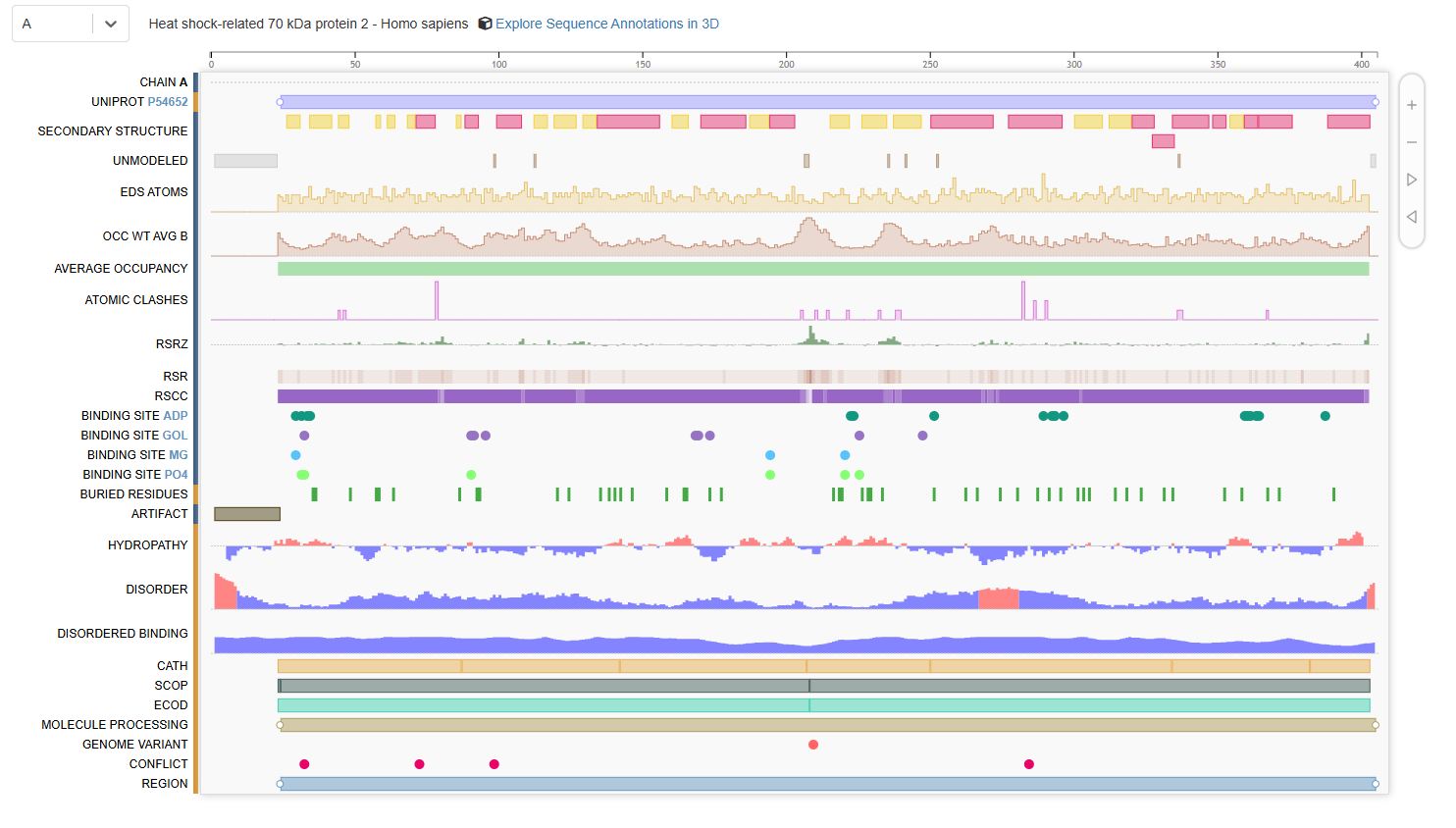Figure 1. Chain A of human 70kDa heat shock protein 2 (Hsp70-2)

The ATPase domain of HSP70-2 belongs to several structure classification families. According to the RCSB PDB annotations for 3I33:

• SCOPe classification: Class: Alpha and beta proteins (a/b); Fold: Ribonuclease H-like motif; Superfamily: Actin-like ATPase domain; Family: Actin/HSP70

• CATH classification: 3.30.420.40 (Nucleotidyltransferase domain 5), 3.30.30.30 (Defensin A-like), and 3.90.640.10 (Actin, Chain A domain 4)

• ECOD classification: Family PF00012 (Hsp70 protein family)

These classifications confirm that this domain shares a common evolutionary origin with actin and other ATPases, which is consistent with its function of binding and hydrolyzing ATP to drive protein folding.

4. Open the structure of your protein in any 3D molecule visualization software:

• PyMol Tutorial
• Visualize the protein as “cartoon”, “ribbon” and “ball and stick”.
• Color the protein by secondary structure. Does it have more helices or sheets?
• Color the protein by residue type. What can you tell about the distribution of hydrophobic vs hydrophilic residues?
• Visualize the surface of the protein. Does it have any “holes” (aka binding pockets)?

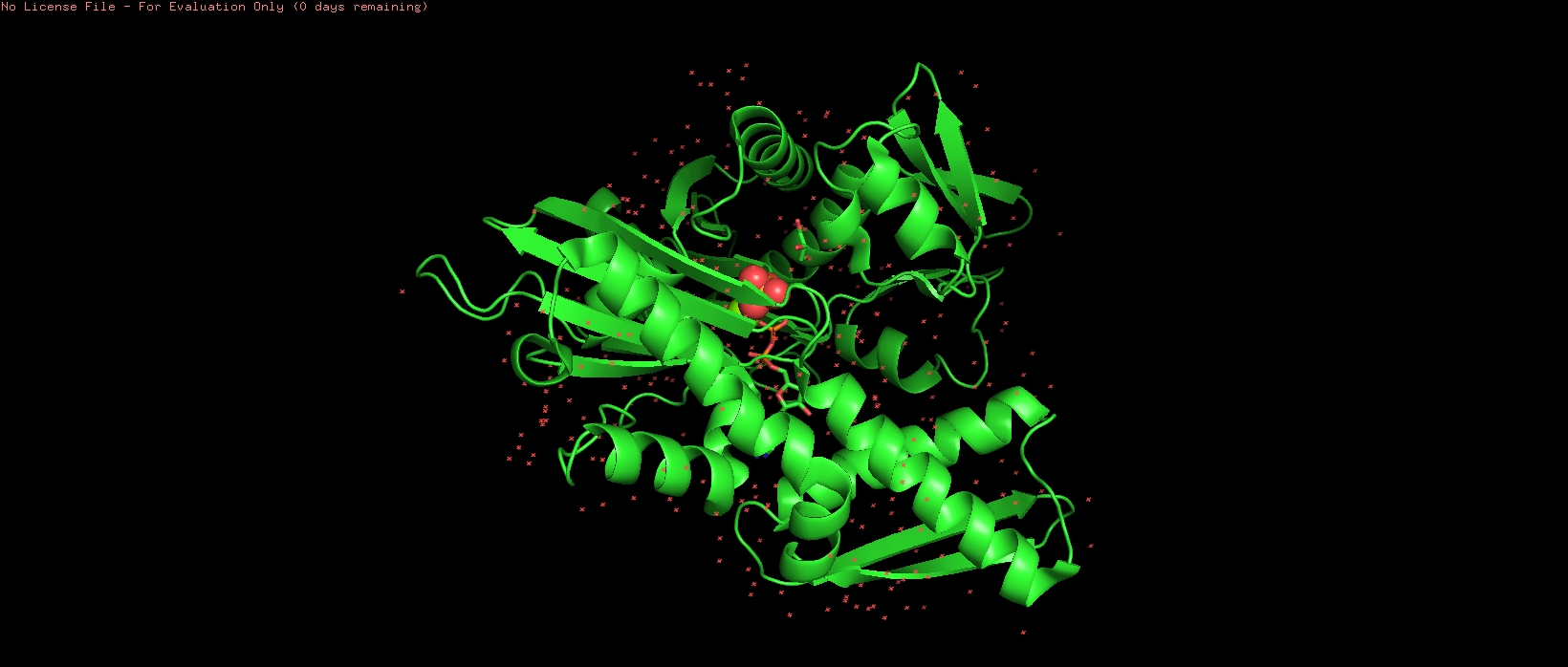Figure 2. Default representation of the HSP70-2 ATPase domain (3I33) in PyMOL before any styling changes.

The initial view of the protein (PDB ID: 3I33) in PyMOL shows the default representation.

Figure 3. Cartoon representation of HSP70-2 ATPase domain, showing alpha helices (spirals) and beta strands (arrows).

The cartoon representation highlights the secondary structure elements: alpha helices are shown as coiled ribbons, and beta sheets as flat arrows. This view makes it easy to see the overall fold and arrangement of structural motifs.

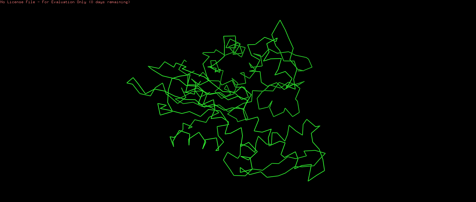Figure 4. Ribbon representation of the HSP70-2 ATPase domain, illustrating the protein backbone trajectory.

The ribbon representation traces the protein backbone as a smooth, continuous ribbon, emphasizing the path of the polypeptide chain. Unlike the cartoon, it does not distinguish between helix and sheet but provides a clean, elegant view of the overall topology.

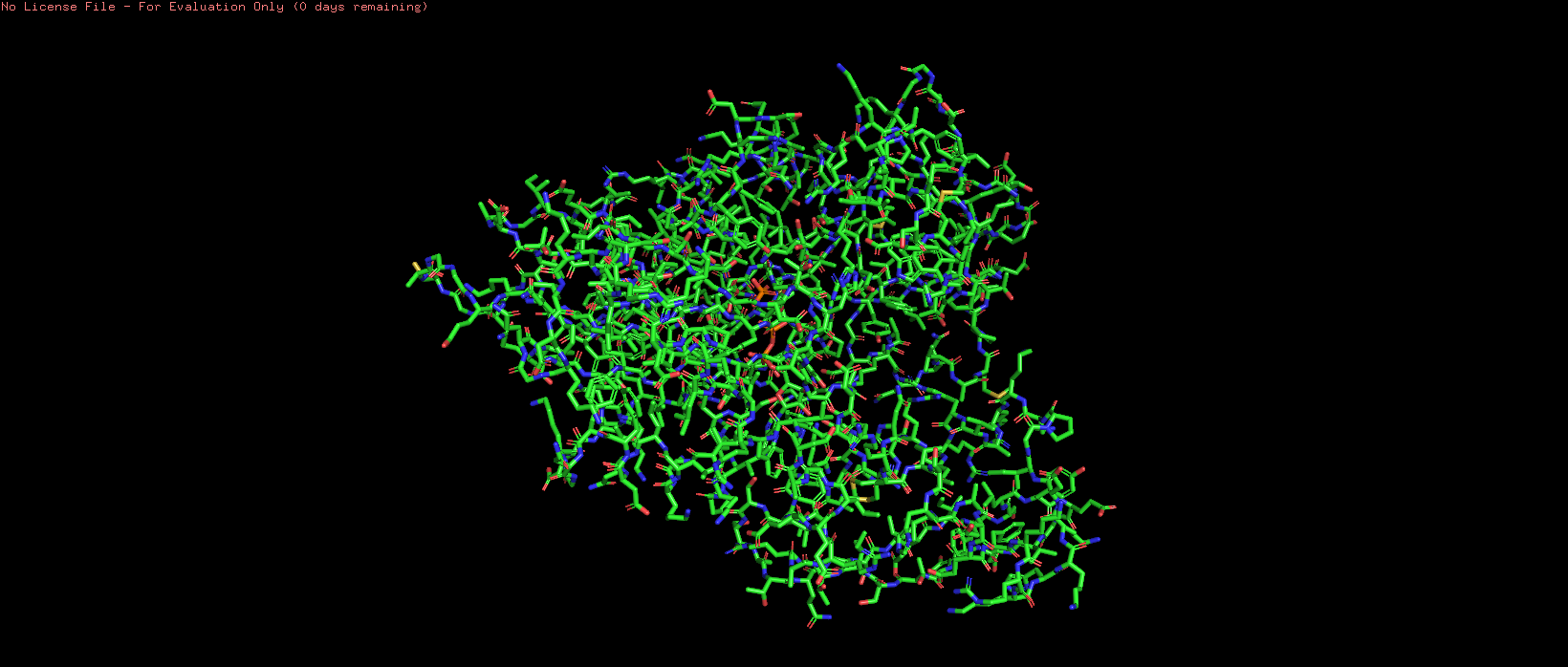Figure 5. Ball and stick representation of HSP70-2, showing individual atoms and bonds.

The ball and stick representation shows individual atoms as spheres and bonds as sticks, revealing the detailed atomic structure. This view is particularly useful for examining side chain orientations and interactions within the active site.

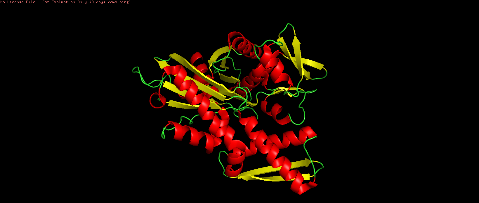Figure 6. HSP70-2 ATPase domain colored by secondary structure (red = alpha helix, yellow = beta sheet, green = loop).

The protein is colored by secondary structure: alpha helices in red, beta sheets in yellow, and loops/turns in green. This color scheme clearly distinguishes the different secondary structure elements and their distribution throughout the domain. Based on the atom count from PyMOL, there are 1,368 atoms in alpha helices and 845 atoms in beta sheets. Therefore, the HSP70-2 ATPase domain contains more alpha helices than beta sheets. This is consistent with the structure of the actin-like ATPase fold, where helices surround a central beta-sheet core.

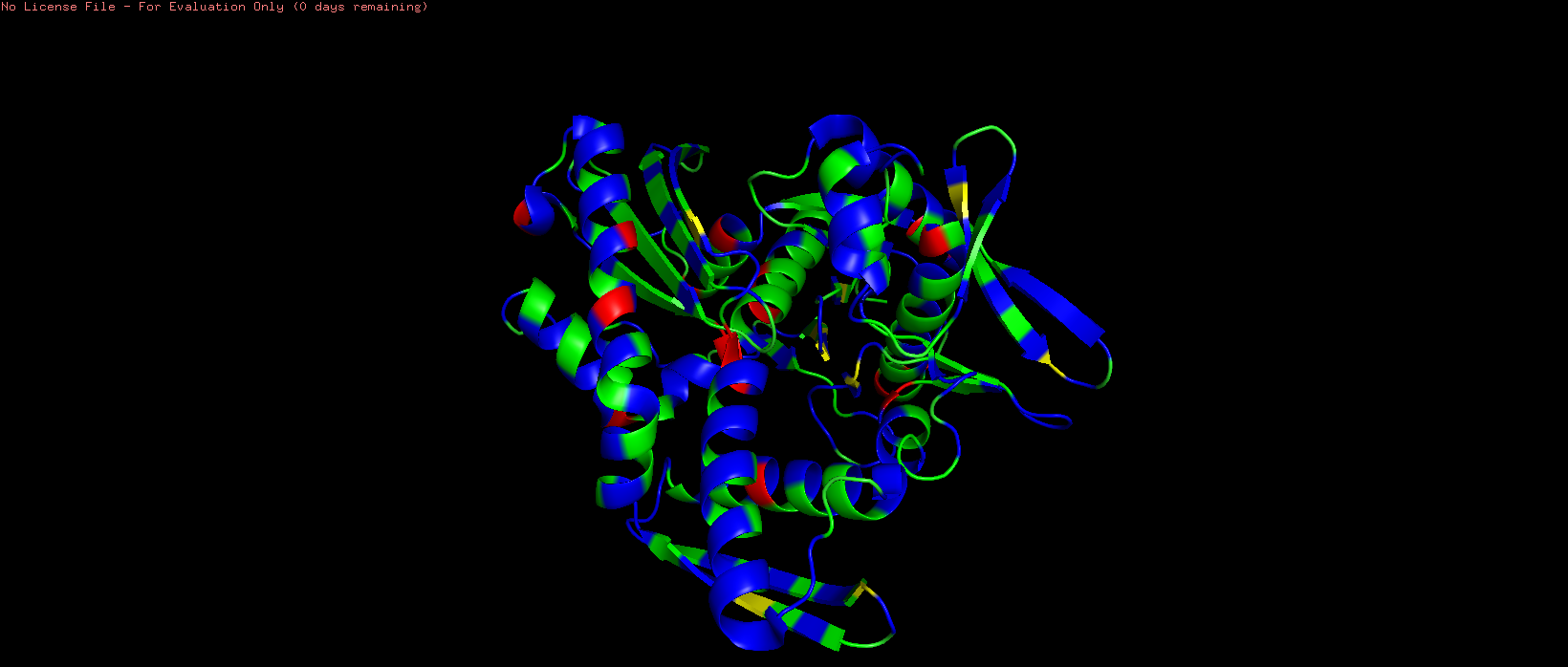Figure 7. HSP70-2 ATPase domain colored by residue hydrophobicity (red = most hydrophobic, blue = hydrophilic).

The protein is colored by residue type using the Eisenberg hydrophobicity scale, where hydrophobic residues (Ile, Leu, Val, Phe, Trp, Met, Ala) appear in shades of red and orange, while hydrophilic residues (charged and polar amino acids) appear in shades of white and blue. This color scheme reveals that hydrophobic residues are predominantly buried within the protein core, while hydrophilic residues are more exposed on the surface. The distribution of hydrophobic and hydrophilic residues follows the typical pattern of a soluble globular protein. Hydrophobic residues (Ile, Leu, Val, Phe, Trp, Met, Ala) are primarily located in the interior of the protein, forming a stable hydrophobic core that drives proper folding through the hydrophobic effect . In contrast, hydrophilic residues (Arg, Lys, Asp, Glu, Asn, Gln, Ser, Thr) are predominantly exposed on the protein surface, where they can interact favorably with the surrounding water molecules. This arrangement is essential for protein solubility and stability. Interestingly, the nucleotide-binding pocket contains a mix of both hydrophobic and hydrophilic residues.

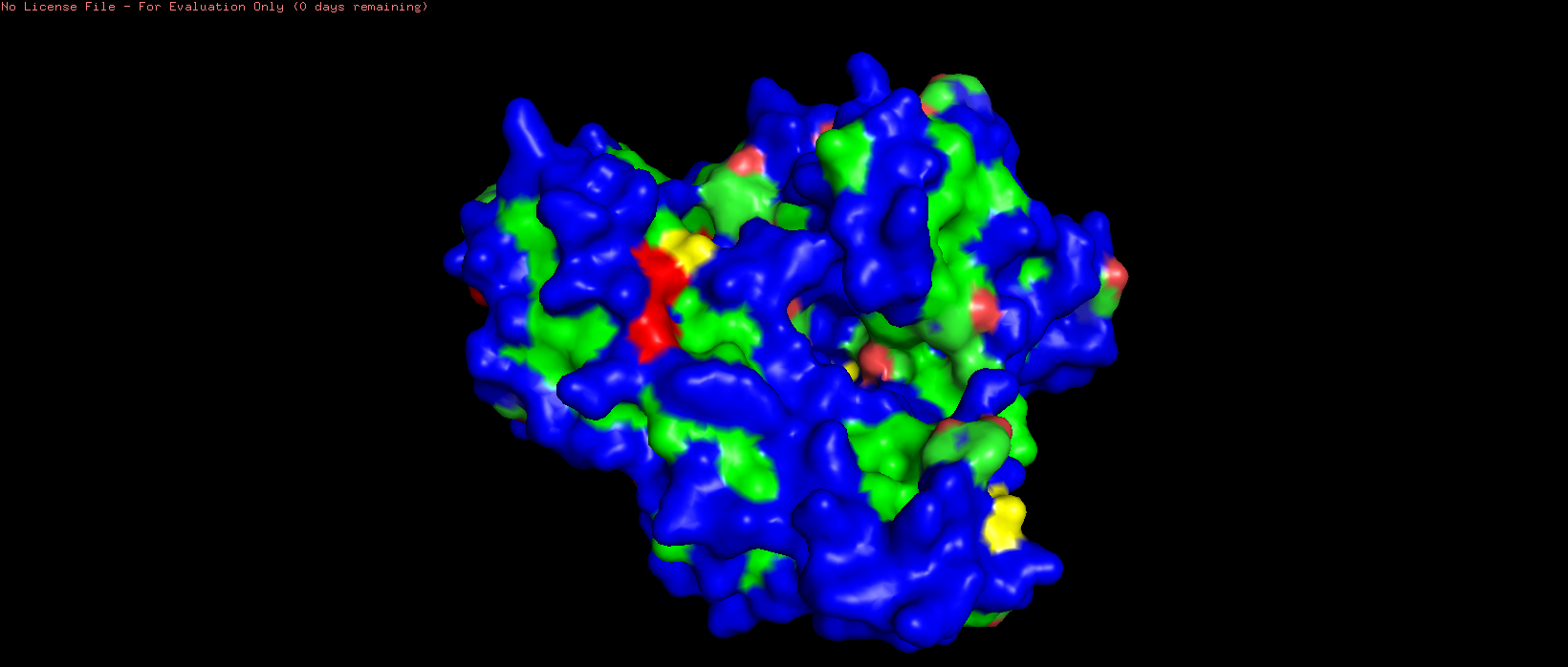Figure 8. Surface representation of HSP70-2 ATPase.

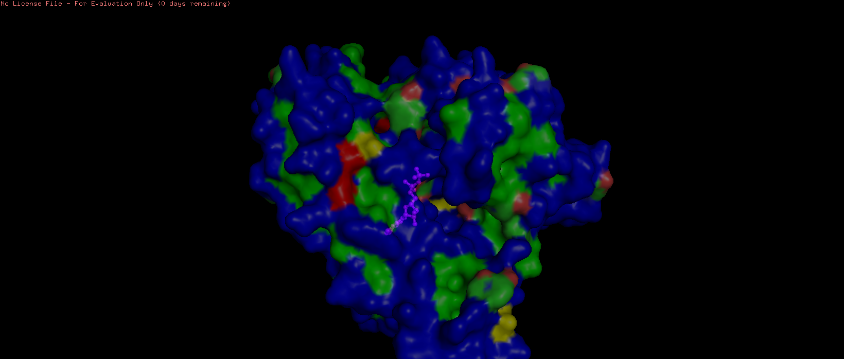Figure 9. Surface representation of HSP70-2 ATPase domain showing the ADP in magenta (sticks and spheres) at transparency 0.5.

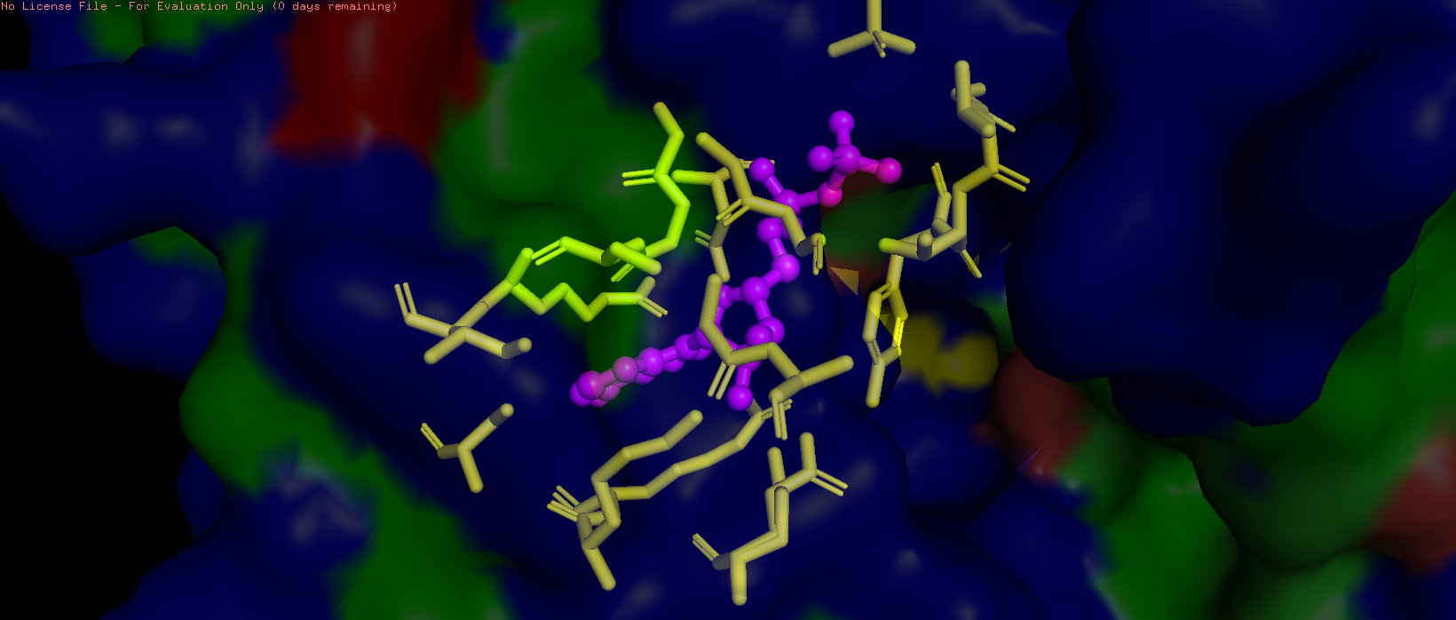Figure 10. Pocket residues within 4.2 Å of ADP are highlighted in yellow.

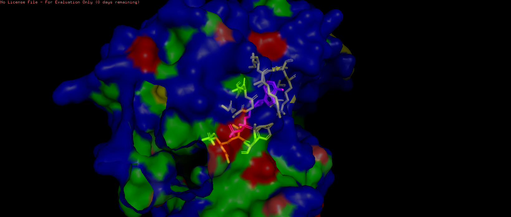Figure 11. Surface representation of HSP70-2 ATPase domain showing the ADP-binding pocket (transparency = 0.5).

The HSP70-2 ATPase domain contains a prominent binding pocket that accommodates ADP. This pocket is located in the deep cleft between subdomains I and II of the ATPase domain. The pocket is lined with specific residues that coordinate nucleotide binding. The adenine ring binds in a hydrophobic region formed by residues such as Ile, Leu, and Val. The ribose and phosphate groups interact with polar and charged residues including Asp, Glu, and Lys. A magnesium ion is coordinated within the pocket to assist with phosphate binding. The presence of this pocket is functionally critical, as HSP70 proteins hydrolyze ATP to provide energy for their chaperone activity helping other proteins fold correctly. Additional small molecules in the structure, including glycerol (GOL) and phosphate ions (PO4), are also bound near the pocket, further confirming its role as the primary ligand-binding site.

Part C. Using ML-Based Protein Design Tools

C1. Protein Language Modeling

1. Deep Mutational Scans

a. Use ESM2 to generate an unsupervised deep mutational scan of your protein based on language model likelihoods. b. Can you explain any particular pattern? (choose a residue and a mutation that stands out) c. (Bonus) Find sequences for which we have experimental scans, and compare the prediction of the language model to experiment.

I used ESM2 (esm2_t33_650M_UR50D) to perform an unsupervised deep mutational scan of the HSPA2 ATPase domain (PDB: 3I33). For each position in the 380-residue sequence, the model masked that position and computed the log-likelihood ratio (LLR) of each possible amino acid substitution relative to the wild-type residue. A negative LLR indicates the mutation is disfavored by the language model (predicted deleterious), while a positive LLR indicates the substitution may be tolerated or even preferred.

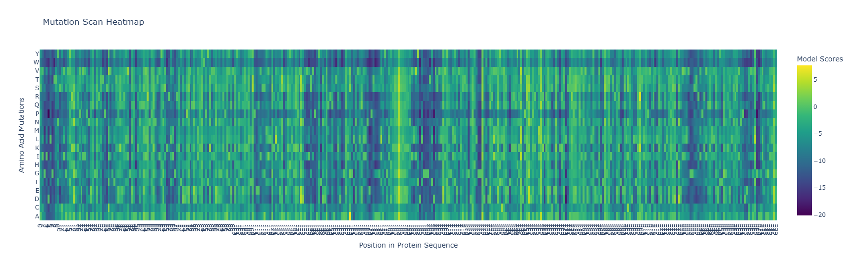
The heatmap reveals a heterogeneous conservation landscape. Most positions show moderate tolerance (blue-green, LLR ~0 to -5), but a subset of columns reach the most extreme negative scores (LLR approaching -20, deep purple), indicating near-complete intolerance to any mutation. Notably, these highly constrained columns are scattered across the sequence rather than forming one continuous block. This is consistent with the known architecture of the Hsp70 ATPase domain, where the nucleotide-binding site is assembled from multiple loops that are distant in sequence but converge in three-dimensional space. The P (proline) row is among the darkest across most columns. This is a universal feature of protein mutational landscapes. Proline introduces a rigid kink in the backbone and eliminates the NH hydrogen bond donor, making it disruptive nearly everywhere except positions that naturally accommodate it. A region in the middle of the sequence shows a streak of yellow, indicating a position where ESM2 actually prefers a different amino acid over the wild-type. This likely corresponds to a surface-exposed, variable loop where natural Hsp70 homologs show sequence diversity, and the language model has learned that alternative residues are more common at this position across evolution. Among the most striking individual mutations in the scan is any substitution at the conserved Glycine within the Walker A motif (GIDLGTTYSCVGxxGKT). The G→P mutation at this position is predicted to be among the most deleterious in the entire protein (approaching LLR = -20). This is mechanistically justified since the P-loop Glycine requires backbone flexibility to adopt the conformation that cradles the phosphate groups of ADP/ATP. Proline would rigidly lock this backbone, directly disrupting nucleotide binding. The 3I33 crystal structure, which captures HSPA2 in complex with ADP and inorganic phosphate, shows this glycine positioned directly adjacent to the bound ligand, confirming its functional importance.

2. Latent Space Analysis

a. Use the provided sequence dataset to embed proteins in reduced dimensionality. b. Analyze the different formed neighborhoods: do they approximate similar proteins? c. Place your protein in the resulting map and explain its position and similarity to its neighbors.

I used the SCOP ASTRAL database (release 2.08, 40% sequence identity cutoff) as my sequence dataset, which contains ~15,000 diverse protein sequences spanning the known structural universe. Sequences were embedded using ESM2 and reduced to 3D using t-SNE for visualization. The notebook as provided would have taken an estimated 41 hours to run on the full SCOP dataset using the esm2_t33_650M_UR50D model (650 million parameters), processing sequences one by one on a free Colab T4 GPU. Two modifications were made to make this computationally feasible. Instead of embedding all ~15,000 SCOP sequences, I randomly subsampled 500 sequences (random seed=42 for reproducibility), then appended my protein of interest (HSPA2, 3I33) as the 501st sequence to ensure it would appear in the final map. This reduced runtime from ~41 hours to ~30 seconds. I also switched from esm2_t33_650M_UR50D to esm2_t6_8M_UR50D (8 million parameters) for the embedding step. The smaller model produces 320-dimensional embeddings vs 1280-dimensional, and is substantially faster per sequence. Random subsampling means the neighborhood of any given protein depends partly on which 500 sequences happened to be drawn, a different random sample would produce a somewhat different map and potentially different nearest neighbors. The smaller model captures less nuanced sequence information than the 650M model, which may reduce the biological precision of the clustering. These are important caveats to keep in mind when interpreting the results. For a more rigorous analysis, one would embed the full dataset with the larger model, which would require either a more powerful GPU or batch processing overnight.

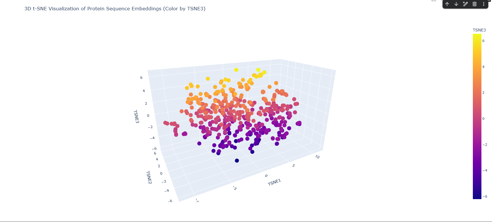
This is the plot produced by the original notebook code, where each dot represents one protein sequence and color corresponds to the value of the third t-SNE component (TSNE3), ranging from deep purple (most negative) to yellow (most positive). This coloring does not represent any biological annotation, it is purely geometric, showing how proteins are distributed along the third axis of the reduced space. The plot shows a broad, continuous cloud of ~500 proteins with some denser and sparser regions, and a general gradient from purple at the bottom to yellow at the top reflecting the TSNE3 axis.

Because the original plot gave no way to locate my specific protein among 501 identical-looking dots, I modified the visualization code with help from Claude to highlight HSPA2 in red while all other SCOP proteins remain blue. This makes it immediately clear where HSPA2 sits in the embedding landscape relative to the broader protein universe.

# Create a color label for each sequence
colors = ['HSPA2 (our protein)' if 'HSPA2' in ann else 'SCOP protein' 
          for ann in annotations]

# Map to discrete colors
color_discrete_map={'HSPA2 (our protein)': 'red', 'SCOP protein': 'steelblue'}

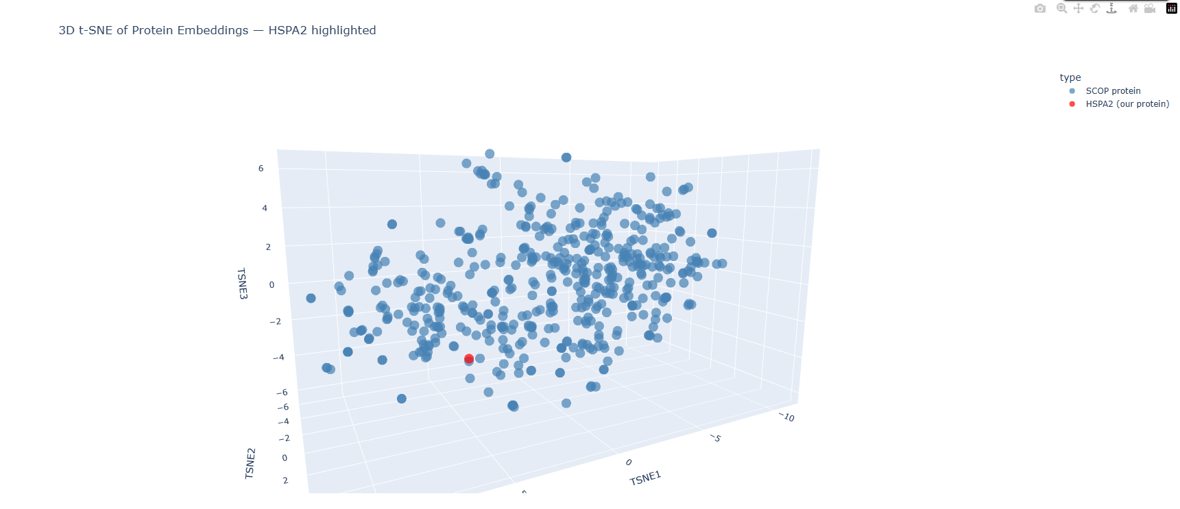
HSPA2 (red dot) is positioned in the lower-middle region of the point cloud, slightly towards the periphery of a local cluster rather than at the center of the overall distribution. It is not completely isolated, there are several blue dots nearby, but it is not buried deep inside a dense cluster either. This peripheral positioning is biologically sensible since the Hsp70 ATPase domain has a distinctive and ancient fold that is structurally shared with many proteins, but the specific human Hsp70 sequence is quite distinct from most other proteins in the randomly sampled SCOP set, naturally placing it somewhat away from the main mass. By hovering over the dots nearest to HSPA2 in the interactive Plotly plot, the closest neighbor was identified as d2w40a2, a protein from Plasmodium falciparum (the malaria parasite) classified under SCOP fold c.55.1, which is the Actin/HSP70 family. The Hsp70 ATPase domain belongs to the actin-like ATPase superfamily, a deeply conserved structural fold shared across actin, hexokinase, sugar kinases, and Hsp70 chaperones across all domains of life. The fact that ESM2 places human HSPA2 nearest to a P. falciparum protein from the same SCOP superfamily without ever being told anything about protein folds, structures, or taxonomy demonstrates that the language model has learned genuine evolutionary and structural relationships purely from patterns in protein sequences. The model has effectively rediscovered that these two proteins, despite coming from organisms separated by over a billion years of evolution, share a common ancestral fold. This validates the core premise of protein language model embeddings, proximity in embedding space approximates biological relatedness. The neighborhoods formed in the t-SNE map do approximate genuinely similar proteins, at least at the level of fold superfamily.

C2. Protein Folding

1. Fold your protein with ESMFold. Do the predicted coordinates match your original structure?

ESMFold is a protein structure prediction model developed by Meta AI that predicts 3D protein structure directly from sequence using a large language model (ESM2) as its backbone, without requiring multiple sequence alignments. It outputs per-residue confidence scores called pLDDT (predicted local distance difference test, 0–100) and a global pTM score (predicted template modelling score, 0–1). Higher is better: pLDDT >90 and pTM >0.9 indicate very high confidence predictions.

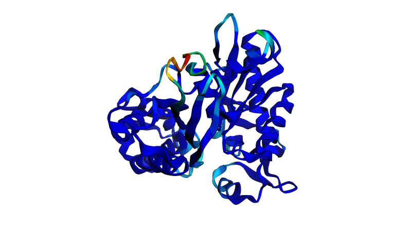
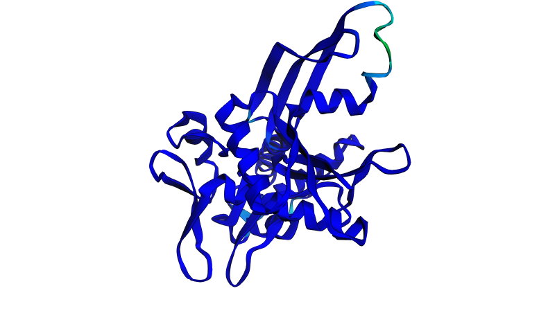
The ESMFold prediction of the wild-type HSPA2 ATPase domain is overwhelmingly deep blue, indicating very high confidence across nearly the entire structure. The characteristic two-lobe architecture of the Hsp70 ATPase domain is clearly visible, the large beta-sheet sandwich and surrounding alpha helices are all well-resolved. The only regions of lower confidence (cyan, green, yellow, red) are a small exposed loop near the nucleotide-binding cleft, which makes sense because this loop is flexible in solution and adopts slightly different conformations in different crystal structures. The ptm is 0.906 and pLDDT is 91.456. The predicted structure matches the known crystal structure (PDB: 3I33) very well. The overall fold, the relative orientation of the two subdomains, and the positions of the major secondary structure elements are all consistent with the experimentally determined coordinates.

2. Try changing the sequence, first try some mutations, then large segments. Is your protein structure resilient to mutations?

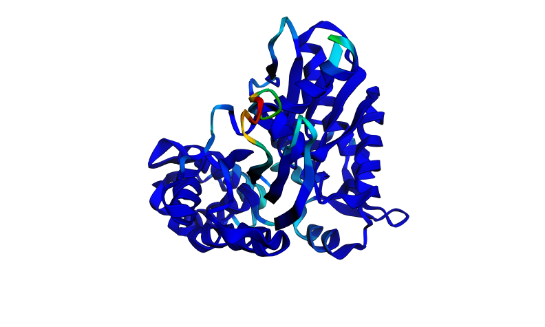
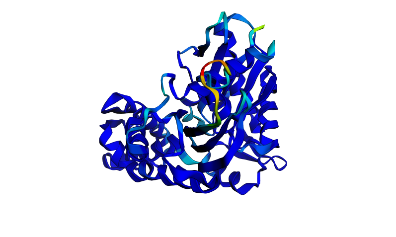
Two mutations were introduced at the most functionally critical residues identified from the ESM2 deep mutational scan: the P-loop glycine (G8A) and the Walker B catalytic aspartate (D→A). These are positions where the DMS scan predicted the most extreme fitness defects, with log-likelihood ratios approaching -20. Strikingly, the predicted structure is almost identical to the wild-type, the ptm score is unchanged (0.906) and the pLDDT drops by only 0.096 points (91.456 → 91.360), which is essentially negligible. The overall fold is completely preserved, with the same small flexible loop showing reduced confidence.

This reveals an important distinction, ESMFold predicts structure, not function. The mutations G8A and D→A are predicted by ESM2 to be severely deleterious to protein fitness, and experimentally they abolish ATPase activity entirely. However, they do not unfold the protein, the backbone scaffold of the ATPase domain is stable enough to maintain its fold even without these catalytic residues. This is a classic example of the difference between structural stability and functional activity. The protein retains its shape but loses its ability to hydrolyse ATP.

A stretch of about 97 residues was deleted from the middle of the sequence, removing part of the interdomain region and the Walker B motif. The result is surprising in that both confidence scores actually improved relative to wild-type (pTM 0.906 → 0.937, pLDDT 91.456 → 95.169), and the structure is almost entirely deep blue with almost no low-confidence regions.

I believe the deleted region included the most flexible loop that was responsible for the low-confidence (red/yellow) region in the wildtype prediction. By removing those residues, ESMFold no longer has to model a disordered, flexible region, so the truncated protein is a more compact, more rigidly foldable domain. The higher confidence scores reflect that the remaining sequence folds very cleanly into a stable structure, not that the deletion is biologically beneficial. However, this truncated protein would almost certainly be non-functional since it is missing critical structural and catalytic elements.

Across all three runs, HSPA2 demonstrates remarkable structural resilience. Point mutations at even the most functionally critical residues do not disrupt the predicted fold, and even a large deletion produces a confident prediction of a compact structure. This reflects the general principle that protein folds are often more tolerant of sequence change than protein functions.

C3. Protein Generation

1. Analyze the predicted sequence probabilities and compare the predicted sequence vs the original one.

Traditional protein folding asks: given a sequence, what is the structure? Inverse folding asks the opposite: given a structure (backbone coordinates), what sequences would fold into it? ProteinMPNN is a graph neural network trained to take the 3D backbone geometry of a protein as input and outputs a probability distribution over amino acids at each position, then samples a new sequence predicted to fold into that same structure. This is a powerful tool for protein design because it allows generation of novel sequences with a desired fold.

I used ProteinMPNN (v_48_020, 48 edges, 0.20Å backbone noise) with the experimentally determined crystal structure of HSPA2 (PDB: 3I33) as input. Settings used:

• Designed chain: A (the full ATPase domain)
• Fixed chain: none
• Sampling temperature: 0.1 (low temperature — sequences stay close to natural amino acid preferences for that backbone)
• Number of sequences: 1

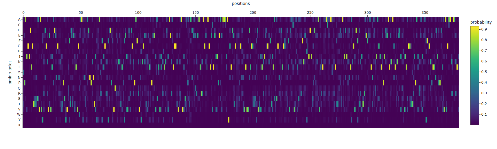
This heatmap shows ProteinMPNN’s predicted probability for each of the 20 amino acids (Y-axis) at every position in the protein (X-axis, positions 0–380). Color ranges from dark purple (probability = 0) to bright yellow (probability = 1).

Most positions have one clear dominant amino acid, at any given column, typically only one or two rows light up with yellow/green while everything else is dark purple. This means ProteinMPNN is highly confident about what amino acid belongs at most positions given the backbone geometry. This makes sense for a well-structured, deeply buried domain like the Hsp70 ATPase fold. Some positions show broader distributions, a handful of columns show multiple amino acids with moderate probabilities (cyan/teal across several rows). These correspond to surface-exposed positions where the backbone geometry is compatible with several different amino acids, reflecting genuine sequence flexibility at those sites. The G row (Glycine) lights up sharply at specific positions, and it is uniquely required wherever the backbone adopts conformations outside the normal Ramachandran space (e.g. tight turns, the P-loop). The L, I, V rows (hydrophobic residues) dominate the core positions, many of the brightest yellow cells are in the L, I, K, and V rows, reflecting the hydrophobic core of the ATPase domain where bulky nonpolar residues are structurally required.

ProteinMPNN generated the following new sequence from the HSPA2 backbone:

MPAIGIDLGTGTSAVAVYRDGRVEVLADEHGNKTIPSYVRFTETEVLVGWDAYNSIADNPKNTIYGARKFLGR KFDDPYVQELKKTLKFKVVDVDGEPYFEVYYKGKTVTLRPEEVLALVIRRLVEVAERALGGTVRRAVITAPAD ADEEEREALRRAGELAGLEVLEIIPEPVAAAIAYGLDETGTEPGNKNVLVVDLGTSSFDVVILRIENGEFTILAVS GDRDLGFNNFVDALVKYLSEKFKKDYGIDITPDEKAVLTLKKAAAKALKELFTNDEAKIDIKNLYKGIDFKTTIT REEAVELNKELIEGILKPIEEALEKAGLKKDEIEHIILVGGTTNFPAIREVIKEYFNGKELLDDIPPDLAVAVGAAK RAARLL

Comparing the two sequences by eye, many positions are clearly different. For example, the N-terminus starts with MPAIGIDLGTGT vs the original PAIGIDLGTTYSC, yet the overall amino acid composition and hydrophobic/hydrophilic patterning is similar. The model has found a different sequence that it predicts will adopt the same backbone geometry.

2. Input this sequence into ESMFold and compare the predicted structure to your original.

Folding the ProteinMPNN-designed sequence with ESMFold produces a structure that is very similar to the original HSPA2 wild-type prediction (ptm: 0.906, pLDDT: 91.456). The scores are nearly identical: ptm: 0.908 and pLDDT: 90.831. The overall fold (the two-lobe architecture, the central beta sheet, the surrounding alpha helices) is preserved in the designed sequence. The same small flexible loop near the nucleotide binding site shows reduced confidence (cyan/red region), just as in the wild-type prediction. The pLDDT drops by only 0.6 points, which is negligible. This is a strong validation result. ProteinMPNN successfully designed a sequence with substantially different amino acids that ESMFold predicts will fold into essentially the same three-dimensional structure. This demonstrates the core principle of inverse folding that protein backbone geometry strongly constrains but does not uniquely determine sequence. Many different sequences can encode the same fold, and ProteinMPNN has learned to navigate this many-to-one mapping.

Part D. Group Brainstorm on Bacteriophage Engineering

I have selected the following goals for engineering the L protein:

1. Increased stability -> improve thermal and proteolytic stability to ensure proper folding and membrane insertion
2. Independence from E. coli DnaJ -> reduce or eliminate reliance on the host chaperone DnaJ for processing, making lysis more robus against host resistance mechanisms

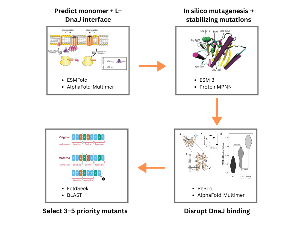
My proposed computation pipeline has 4 stages. The first stage would be to use ESMFold and AlphaFold-Multimer for sequence and structure analysis. This would generate a high-confidence monomeric structure of MS2-L, then model the L–DnaJ complex to identify interface residues. ESMFold provides rapid single-chain predictions and AlphaFold-Multimer gives interface confidence metrics (ipTM) for the complex. The result would be 3D coordinates of L protein monomer and L–DnaJ heterocomplex with per-residue confidence (pLDDT) and interface scores. The second stage would use ESM-3 and PrteinMPNN to run in silico mutagenesis for stability. I would use ESM-3 embeddings to score mutational effects on stability via likelihood changes and identify stabilizing mutations in hydrophobic core regions. I would use ProteinMPNN in fixed backbone mode to redesign surface/exposed residues while preserving the transmembrane helix, improving solubility and folding efficiency. The output would be a ranked list of stabilizing point mutations (e.g., core packing improvements, helix-stabilizing substitutions). The third stage would be to use AlphaFold-Multimer and PeSTo to disrupt L-DnaJ interaction. I would indetify DnaJ-binding hotspots on L using PeSTo’s interface residue predictor, and then design mutations at these interfaces and again predicts the complex with AlphaFold-Multimer to confirm reduced ipTM scores. The output would be mutant sequences predicted to weaken or get rid of DnaJ binding while maintaining monomer stability. The final stage would be to use FoldSeek and BLAST to check if the designed mutants retain the native fold, and to avoid creating unintended homologs to toxic or immunogenic proteins. The output would be 3-5 high-priority mutant candidates for synthesis.

Some potential pitfalls in this pipeline include limited training data on pahge-bacteria chaperone interactions, and stability-activity trade off. ESM-3 and ProteinMPNN are trained on general protein databases, that means that phage-specific constraints, such as transmembrane topology and small protein size, may be underrepresented, leading to suboptimal predictions. Additionally, mutations that increase stability or disrupt DnaJ binding may inadvertently reduce lysis potency as seen in T7 endolysin engineering studies. Experimental validation will be essential to confirm that designed mutants retain function.

The figure below shows the pipeline schematic: