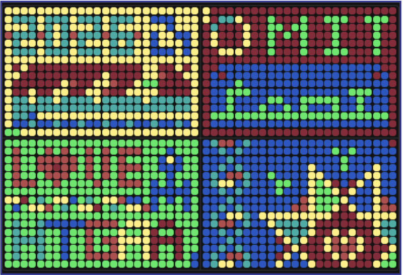
title: ‘DNA Gel Art’ weight: 10 Week 2 Lab: DNA Gel Art This lab was about using restriction digests and gel electrophoresis to make DNA gel art. Instead of only using a gel as a diagnostic tool, we used the positions of DNA bands as a visual medium. The basic idea was that different restriction enzymes cut Lambda DNA into different fragment sizes, and those fragments separate into bands when run through an agarose gel.
Week 6 Lab: Gibson Assembly This lab focused on using PCR, Gibson Assembly, and bacterial transformation to modify a plasmid carrying the amilCP chromoprotein gene. The goal was to introduce targeted color mutations and then transform the assembled plasmids into E. coli so that successful variants could be identified by colony color.
Our group worked on color variants intended to produce magenta and blue colonies. The experiment had several stages: PCR amplification, PCR cleanup, diagnostic gel electrophoresis, Gibson Assembly, transformation, recovery, plating, and colony observation.
I was not able to attend this lab in person because I was traveling for an interview. I informed Ronan ahead of time. A makeup session was not offered because this lab depended on time-sensitive biological materials, including mammalian cells that had already been grown or plated for the scheduled experiment.
Even though I missed the hands-on part, I reviewed the lab materials and thought through what I would have done if I had been there.
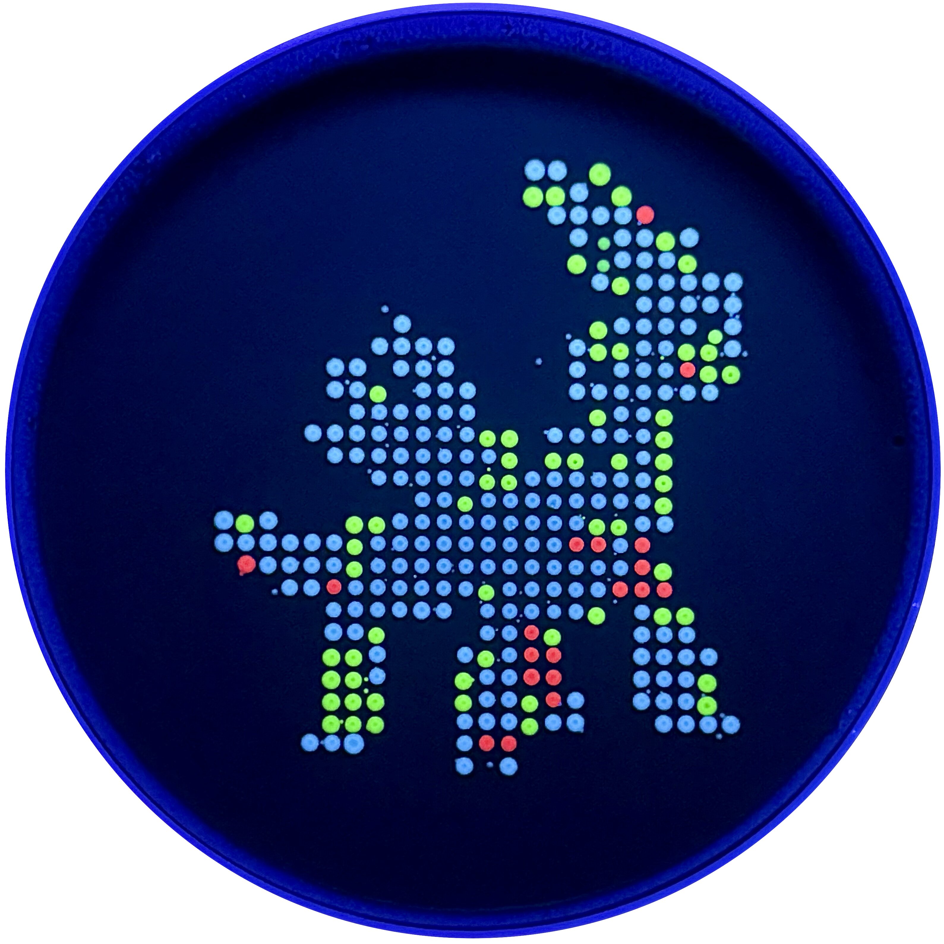
Dialga: A Legendary Pokemon from the Sinnoh region
Subsections of Labs
Cloud Lab
Week 11 Lab: Cloud Lab
DNA art
title: ‘DNA Gel Art’
weight: 10
Week 2 Lab: DNA Gel Art
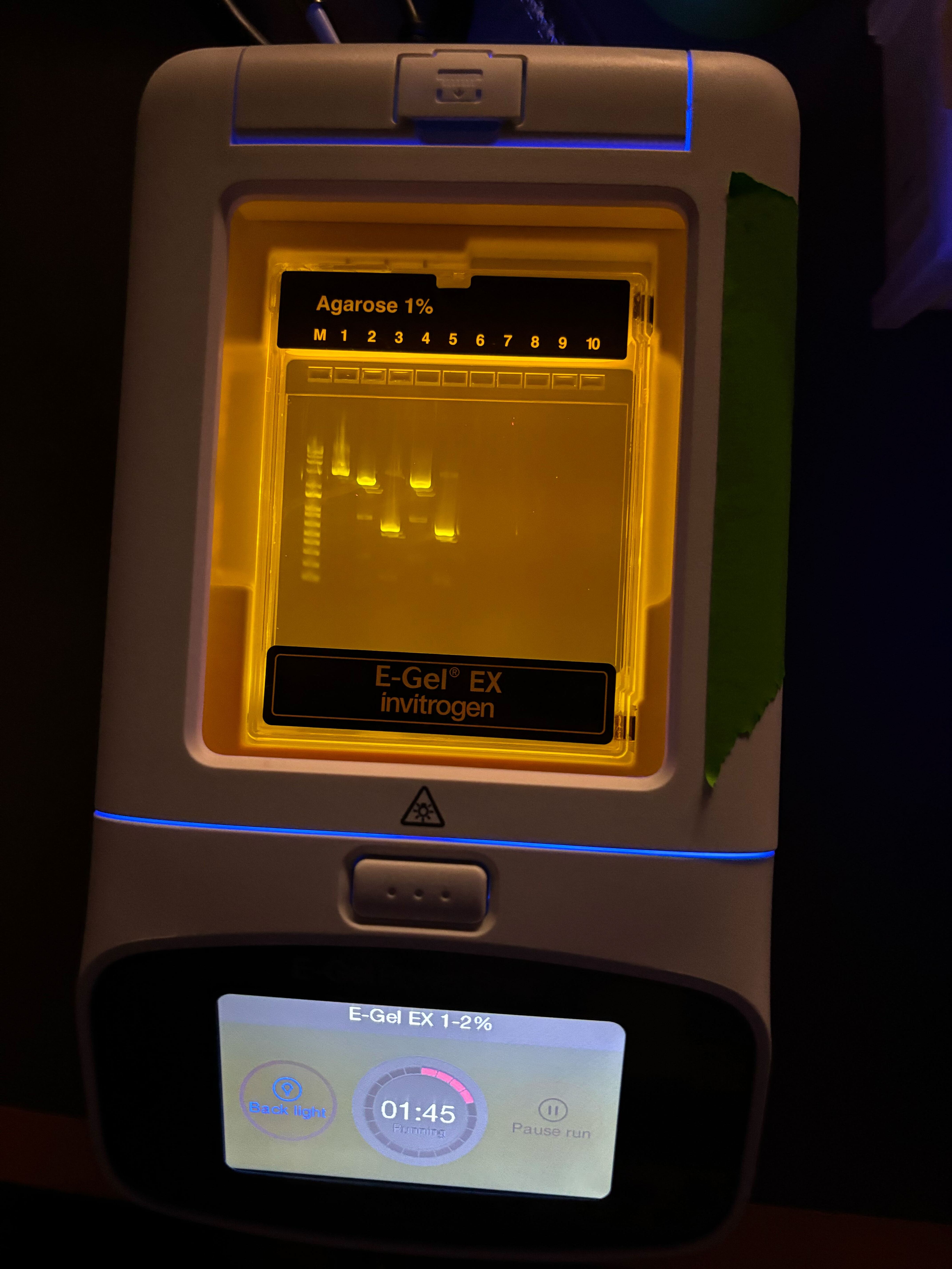
This lab was about using restriction digests and gel electrophoresis to make DNA gel art. Instead of only using a gel as a diagnostic tool, we used the positions of DNA bands as a visual medium. The basic idea was that different restriction enzymes cut Lambda DNA into different fragment sizes, and those fragments separate into bands when run through an agarose gel.
I followed the lab protocol for designing the gel, preparing the restriction digests, casting the agarose gel, loading the samples, running electrophoresis, and imaging the final result.
Goal of the Lab
The goal was to create a visual pattern using DNA bands. Each lane of the gel was supposed to contain a different restriction digest. Since each enzyme cuts Lambda DNA at specific sites, each digest should produce a distinct set of DNA fragment sizes. When run on the gel, those fragments should migrate different distances and create the planned pattern.
This is the same principle used in normal molecular biology. If a DNA sequence is known, restriction digest software can predict what bands should appear. A real gel can then be compared against that prediction.
Design Process
Before the wet-lab steps, I planned the gel design digitally. The design process involved testing combinations of restriction enzymes on Lambda DNA and looking at the predicted band positions.
The enzymes available included:
EcoRI-HF
HindIII-HF
BamHI-HF
KpnI-HF
EcoRV-HF
SacI-HF
SalI-HF
The “HF” versions are high-fidelity restriction enzymes, which are designed to reduce off-target cutting. The visual design was based on choosing enzyme combinations that would create useful bands in each lane.
The important thing I learned is that gel art is not drawn directly. The image comes from fragment sizes. The design has to be translated into enzyme choices, and the enzyme choices then determine the band positions.
Preparing the Agarose Gel
I prepared a 1% agarose gel. The gel was made by mixing agarose powder with 1x TAE buffer.
Component
Amount
Agarose
0.75 g
1x TAE buffer
75 mL
SYBR Safe DNA stain
7.5 uL
The agarose and TAE were heated in the microwave in short pulses until the agarose dissolved and the solution became clear. I swirled the flask between heating steps to help dissolve the agarose evenly.
After the solution cooled slightly, SYBR Safe DNA stain was added. This stain binds to DNA and makes the bands visible under blue light after the gel is run.
The liquid gel was then poured into a casting tray with a comb in place. The comb created the wells where the DNA samples would later be loaded. After the gel solidified, the comb was removed carefully.
Restriction Digest Setup
While the gel was setting, I prepared the restriction digest reactions. Each reaction corresponded to one lane of the gel.
The general digest reaction volume was 20 uL.
Component
Amount
Lambda DNA
3 uL
10x enzyme buffer
2 uL
Restriction enzyme
1 uL per enzyme
Nuclease-free water
to 20 uL total
The Lambda DNA stock was 0.5 ug/uL, so 3 uL gave 1.5 ug DNA. The enzyme buffer was added so the final buffer concentration would be 1x. If a lane used more than one enzyme, I adjusted the water volume so the final reaction volume stayed at 20 uL.
The tubes were labeled by lane number. This mattered because if two tubes were swapped, the gel would no longer match the intended design.
Digest Incubation
After setting up the digest reactions, I incubated the tubes at 37°C for 30 minutes. This allowed the restriction enzymes to cut the Lambda DNA.
During this step, the full Lambda DNA molecule should be cut into smaller fragments. The number and size of fragments depends on the enzyme or enzyme combination in that tube.
Adding Loading Dye
After incubation, I added loading dye to the samples before loading them into the gel.
Loading dye is useful for two reasons. It makes the sample denser so it sinks into the well, and it also provides a visible dye front that helps track the progress of electrophoresis.
The target loading volume per well was 20 uL.
Component
Amount
6x loading dye
3.33 uL
DNA sample
variable
Nuclease-free water
to 20 uL total
Loading the Gel
Once the gel had solidified, I placed it in the electrophoresis box and added 1x TAE buffer until the gel was covered. The wells were placed near the negative electrode because DNA is negatively charged and migrates toward the positive electrode.
I loaded the samples into the wells according to the lane plan. This was one of the harder parts of the lab because the wells are small. The pipette tip has to be close enough to the well to release the sample cleanly, but not so deep that it punctures the gel.
If the loading step goes wrong, the sample can leak out, diffuse, or fail to enter the well properly.
Running the Gel
After loading, I connected the gel box to the power supply and ran the gel. The protocol recommended running at around 80 to 115 V for about 45 minutes.
When the current is running properly, bubbles appear in the buffer. This shows that the circuit is connected and current is passing through the system.
The DNA fragments separate by size as they move through the agarose. Smaller fragments travel farther, while larger fragments stay closer to the wells.
Imaging
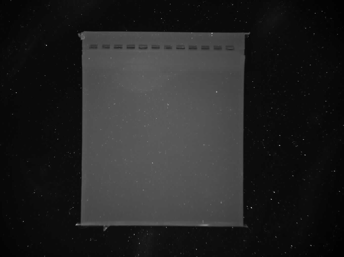
After the gel run, the gel was placed on a blue light transilluminator. Since the gel contained SYBR Safe, DNA bands should fluoresce under blue light and become visible.
In my final image, the gel itself and the wells were visible, but the band pattern was extremely faint or absent. This means the final gel art did not come through clearly.
Potential Failure Modes
Since the final image was mostly blank, there are several possible failure modes.
Possible issue
Why it would matter
Too little DNA loaded
Bands would be too faint to see clearly
DNA was not loaded into the wells correctly
Sample could have floated away or leaked out
Restriction digest did not work
DNA fragments would not match the expected pattern
Enzyme mix-up
The lane pattern would not match the design
Missing or incorrect buffer
Enzymes or electrophoresis may not work properly
Gel ran for the wrong amount of time
Bands could stay near the top or migrate too far
Voltage issue
DNA may not migrate properly
Stain issue
DNA may be present but not visible
Imaging issue
Bands may be weak and not captured well by the camera
Pipetting error
Small volume mistakes can strongly affect final band brightness
Based on the final image, the most likely issues are low DNA visibility, loading problems, or an issue with digestion/loading concentration. Since the wells are visible but the bands are not, the gel itself formed correctly, but the DNA signal did not show up clearly.
Technical Understanding
The lab helped me understand why gel electrophoresis works. DNA has a negatively charged phosphate backbone, so it moves toward the positive electrode in an electric field. The agarose gel acts like a molecular sieve. Smaller DNA fragments pass through the gel more easily and move farther, while larger fragments move more slowly.
Restriction enzymes make the band pattern predictable. Each enzyme recognizes specific DNA sequences and cuts at those sites. If we know the Lambda DNA sequence, we can predict the sizes of fragments produced by each enzyme. The gel result should then show bands corresponding to those predicted fragment sizes.
In this lab, that same molecular biology logic was used creatively. Instead of asking “is this plasmid correct?”, we asked whether enzyme choices could produce a visual pattern.
Reflection
Even though my final DNA art did not work well, this lab helped me understand the full gel electrophoresis workflow. I got practice preparing an agarose gel, setting up restriction digests, adding loading dye, loading wells, running the gel, and imaging the result.
The most difficult part was the precision required. Small errors in pipetting, labeling, loading, or timing can make the final gel unclear. I also saw that a gel result depends on many steps working together. If the design is correct but the DNA is not visible, the final art still fails.
The main takeaway for me was that gel electrophoresis is both conceptually simple and experimentally delicate. The idea is straightforward: cut DNA, separate fragments, and visualize bands. But getting clean bands requires careful execution at every step.
Final Result
My final result did not really show the intended DNA art pattern. The gel image was mostly blank, with the wells visible at the top but very little clear banding across the gel.
Even though the final image did not work well, the lab was still useful because it showed how many steps have to work correctly for a gel to produce a clear image.
Gibson Assembly Lab
Week 6 Lab: Gibson Assembly
This lab focused on using PCR, Gibson Assembly, and bacterial transformation to modify a plasmid carrying the amilCP chromoprotein gene. The goal was to introduce targeted color mutations and then transform the assembled plasmids into E. coli so that successful variants could be identified by colony color.
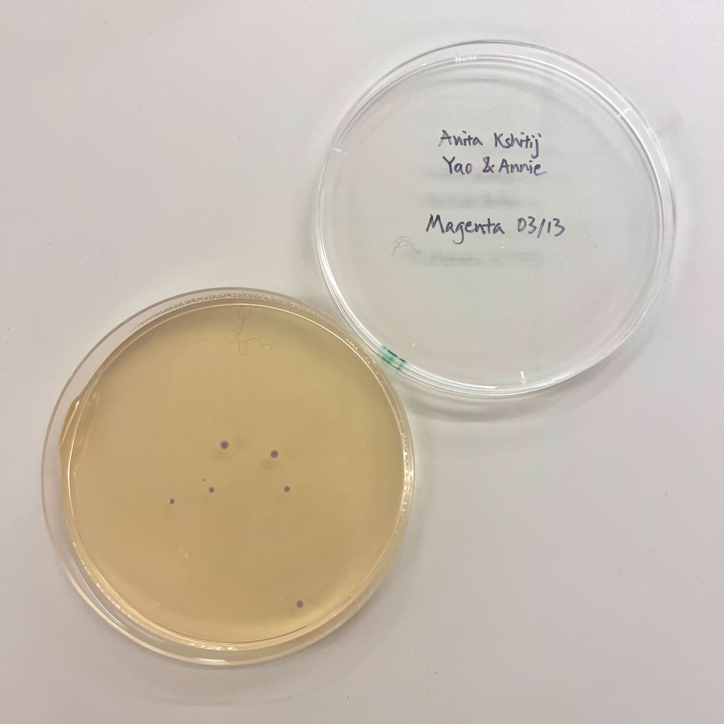
Our group worked on color variants intended to produce magenta and blue colonies. The experiment had several stages: PCR amplification, PCR cleanup, diagnostic gel electrophoresis, Gibson Assembly, transformation, recovery, plating, and colony observation.
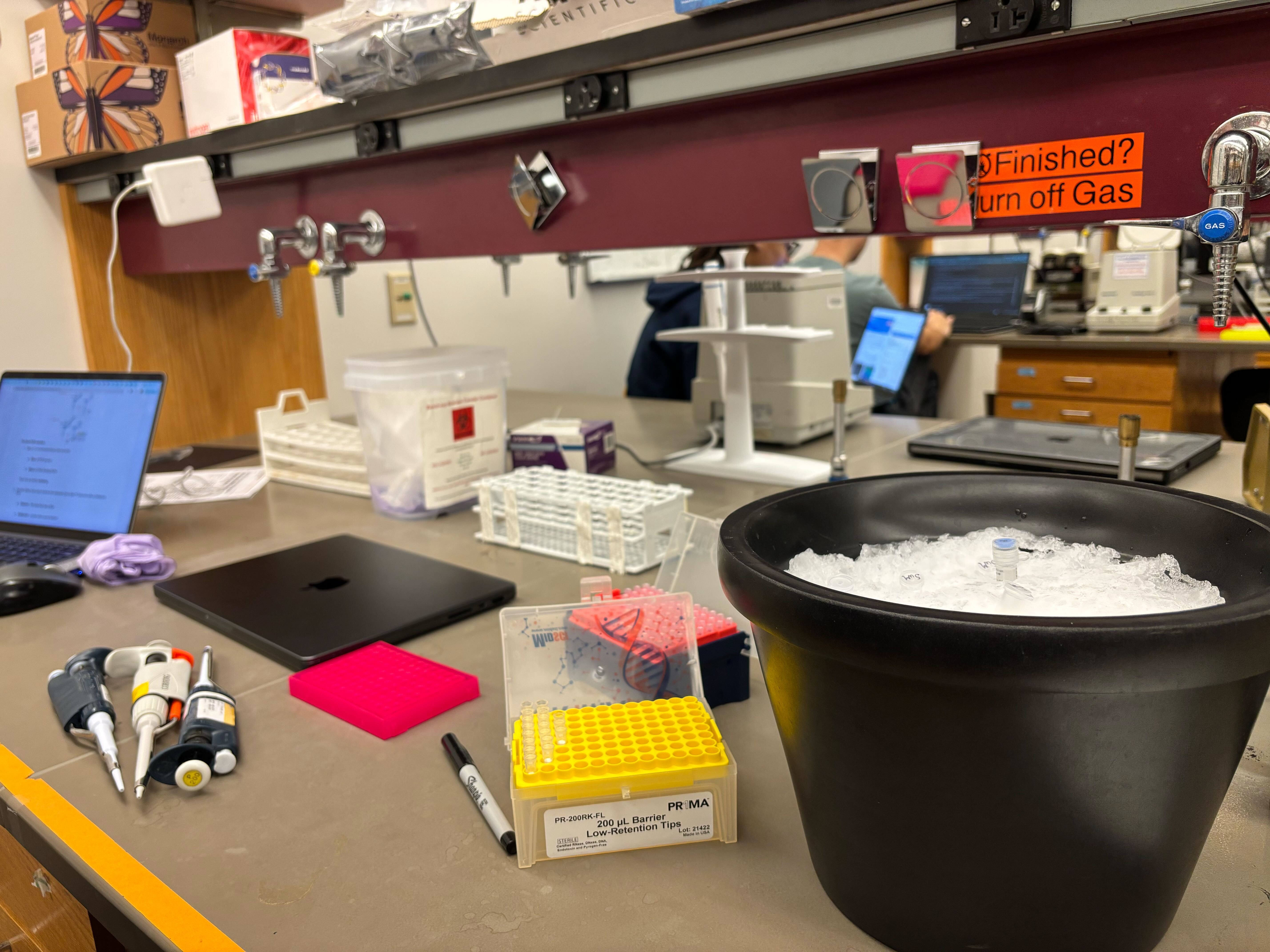
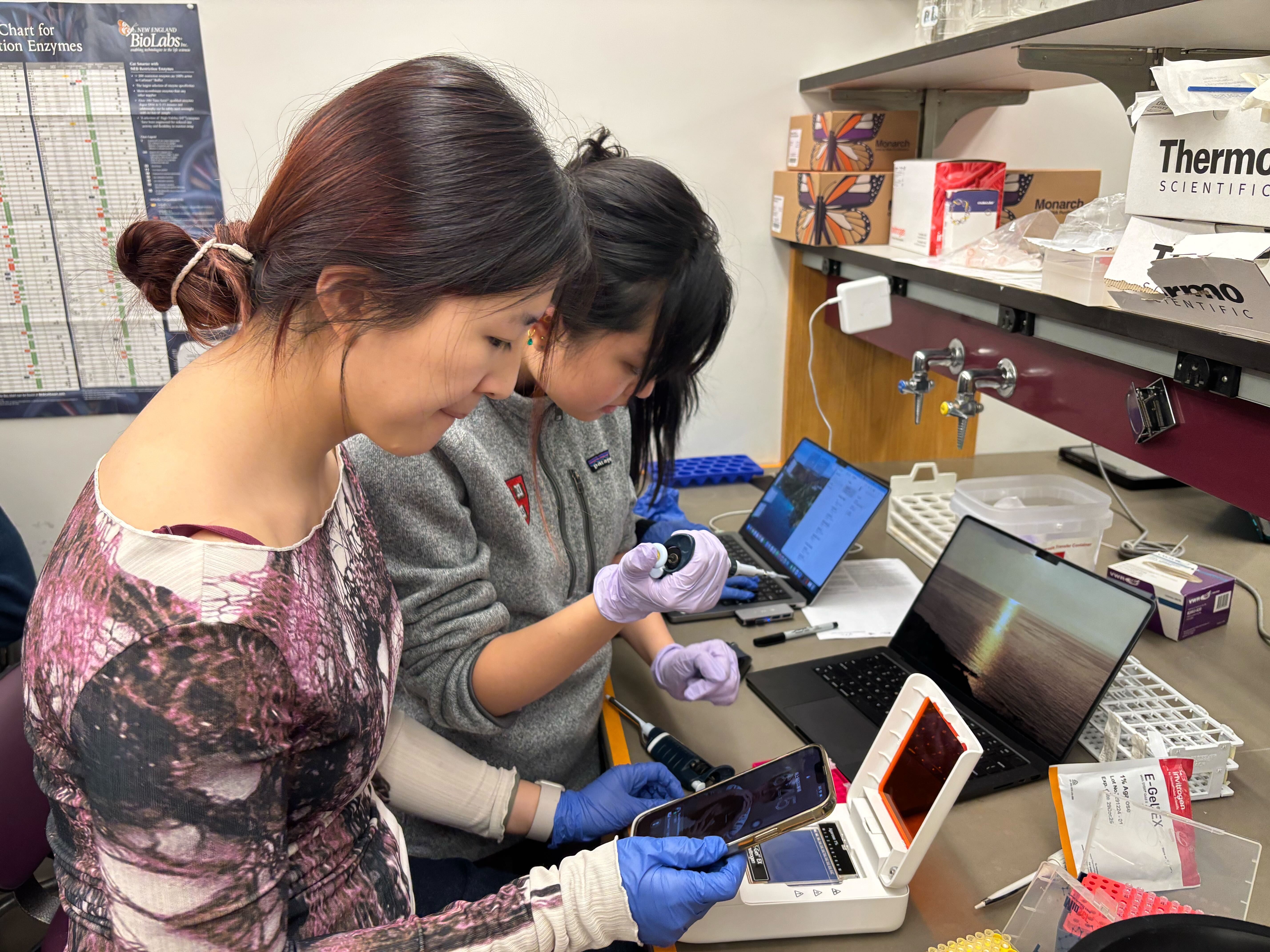
Photos
Here are the photos I took during the lab.
Overall Strategy
The basic idea was to split the plasmid into two PCR products and then put it back together with a designed mutation. One PCR reaction amplified the larger backbone region of the plasmid, and the other amplified the color insert region containing the mutation near the chromoprotein sequence.
After PCR, the fragments were purified and checked on a gel. If the fragments were present at the expected sizes, they could be combined using Gibson Assembly. Gibson Assembly uses overlapping ends between DNA fragments to join them into one circular plasmid. The assembled plasmid was then transformed into chemically competent E. coli cells and plated on antibiotic plates.
Part 1: PCR Setup
We ran two PCR reactions from the mUAV plasmid template.
The first reaction amplified the backbone fragment. This contained the plasmid parts needed for propagation and expression, such as the origin of replication, chloramphenicol resistance, promoter, and ribosome binding site.
The second reaction amplified the color insert fragment. This contained the region around the amilCP chromoprotein gene. The forward primer introduced the color mutation, so the PCR product was not just copying the original sequence. It was also adding the designed change.
Each 25 uL PCR reaction used:
Component
Amount
Template DNA, 38.5 ng/uL
0.8 uL
Forward primer, 5 uM
2.5 uL
Reverse primer, 5 uM
2.5 uL
Phusion HF PCR Master Mix
12.5 uL
Nuclease-free water
to 25 uL
Phusion polymerase was used because it is high-fidelity, which matters when the goal is to create a specific mutation without adding many unintended errors.
PCR Thermocycler Conditions
The backbone and color-insert reactions used different annealing and extension conditions because the fragments had different sizes and primer properties.
Backbone PCR
98°C for 30 seconds
26 cycles:
98°C for 10 seconds
57°C for 25 seconds
72°C for 1.5 minutes
72°C for 5 minutes
12°C hold
Color Insert PCR
98°C for 15 seconds
26 cycles:
98°C for 10 seconds
53°C for 20 seconds
72°C for 15 seconds
72°C for 5 minutes
12°C hold
The backbone needed a longer extension step because it was the larger fragment. The color insert was shorter, so the extension time was much shorter.
Part 1a: PCR Product Cleanup
After PCR, the products were purified using a Zymo DNA Clean & Concentrator kit. This step removed primers, salts, enzymes, and other leftover PCR components that could interfere with later assembly.
For each sample, the PCR product was mixed with DNA binding buffer and loaded onto a spin column. The DNA binds to the column under the buffer conditions. After centrifugation and washing, the DNA was eluted in a small volume of nuclease-free water.
The cleanup workflow was:
Mix 20 uL PCR product with 100 uL DNA binding buffer.
Load onto a ZymoSpin column.
Centrifuge to bind DNA to the column.
Wash twice with 200 uL DNA wash buffer.
Elute DNA in 6 uL nuclease-free water.
The small elution volume helped keep the DNA concentrated for Gibson Assembly.
Part 1b: Diagnostic Gel Electrophoresis
After purification, we ran a diagnostic gel to check whether the PCR reactions produced fragments of the expected sizes. For each sample, 2 uL of purified DNA was mixed with 18 uL water before loading. A pre-diluted DNA ladder was also loaded, and the original mUAV plasmid was used as a reference.
The gel was useful because it gave a quick quality check before assembly. If the backbone and insert bands appeared at the expected positions, that meant the PCR products were likely usable. If a reaction had no band or many nonspecific bands, Gibson Assembly would probably fail or produce the wrong construct.
In our gel image, visible bands appeared in the expected lanes. That suggested that at least some PCR product was present and that the fragments could be carried forward into assembly.
Part 2a: Gibson Assembly
The purified backbone and color-insert fragments were combined using Gibson Assembly Master Mix. Gibson Assembly works because the DNA fragments are designed to have overlapping ends. These overlaps allow the fragments to find each other and be joined into a complete circular plasmid.
The reaction was set up in 10 uL total volume and incubated at 50°C for 15 minutes. After the incubation, 100 uL nuclease-free water was added to dilute the assembly product before transformation.
Mechanistically, Gibson Assembly has four main steps:
An exonuclease chews back the 5’ ends of DNA fragments.
Complementary single-stranded overlaps anneal to each other.
A polymerase fills in missing bases.
A ligase seals the remaining nicks.
This produces a circular plasmid containing the backbone and the mutated color insert.
Part 2b: Transformation
The Gibson Assembly products were transformed into chemically competent DH5α E. coli using heat shock.
The transformation workflow was:
Thaw competent cells on ice for about 10 minutes.
Add 4 uL diluted Gibson Assembly product to 20 uL competent cells.
Incubate on ice for 30 minutes.
Heat shock at 42°C for 45 seconds.
Return cells to ice for 5 minutes.
Add 100 uL SOC media.
Recover with shaking for 60 minutes.
Plate 100 uL on selective agar plates.
Incubate plates at 37°C.
The heat shock step helps plasmid DNA enter the competent cells. The SOC recovery step gives cells time to recover and begin expressing the antibiotic resistance gene before they are placed on selective plates.
Results
The final colony count was low overall. The blue plate showed a small partial success, with a few visibly blue colonies. The magenta plates did not show clear magenta colonies. The colonies that did grow on those plates may have been untransformed, incorrectly assembled, or reverted toward the original purple amilCP color.
The result suggests that at least one assembly or transformation condition worked partially, but the efficiency was low. Possible reasons include low PCR yield, poor fragment ratio in Gibson Assembly, DNA loss during cleanup, inefficient transformation, or mutations not producing the intended visible color.
Reflection
This lab helped me understand how DNA design turns into an actual biological test. Before this, I thought of a mutation mainly as a sequence edit. In practice, the mutation had to pass through many physical steps: primer design, PCR amplification, cleanup, gel checking, Gibson Assembly, transformation, recovery, and plating.
The most useful checkpoint was the gel, because it showed whether the PCR step produced DNA fragments before we moved on to assembly. The plate result was also useful because it gave a biological readout of the whole workflow. Even if the gel looks reasonable, the construct still has to assemble correctly, enter cells, and express the intended chromoprotein.
The low colony count also showed how many things can reduce success in cloning. A weak final result does not necessarily mean one single step failed. It could come from small losses or inefficiencies across multiple steps. Overall, this lab made the full cloning pipeline much clearer to me.
Neuromorphic Circuits and Biomaterials
I was not able to attend this lab in person because I was traveling for an interview. I informed Ronan ahead of time. A makeup session was not offered because this lab depended on time-sensitive biological materials, including mammalian cells that had already been grown or plated for the scheduled experiment.
Even though I missed the hands-on part, I reviewed the lab materials and thought through what I would have done if I had been there.
Lab Goal
The lab was about building neuromorphic genetic circuits in mammalian cells. The word “neuromorphic” here does not mean that the cells are literally neurons. It means that the circuit is designed to process information in a more dynamic way than a simple on/off reporter.
Instead of just putting a fluorescent protein after a promoter, the circuit uses regulatory parts that interact with each other before producing an output. That makes the behavior depend on combinations of inputs, expression levels, and timing.
What I Would Have Tried
If I had attended the lab, I would have kept my circuit fairly simple. Since transfection itself can be noisy, I think it would be better to design something that is easy to debug rather than something too clever.
I would have tried a two-input circuit where Csy4 and CasE act as the main regulatory inputs, and mNeonGreen is the final output. I would also include separate fluorescent markers for the two input groups so that I could tell whether the cells actually received and expressed those inputs.
Group
Part
Why I would include it
X1
Csy4
First regulatory input
X1
mKO2
Marker showing X1 was expressed
X2
CasE
Second regulatory input
X2
eBFP2
Marker showing X2 was expressed
Output
Csy4_rec_CasE
Interaction module between the regulatory parts
Output
CasE_rec_mNeonGreen
Final green output
The main reason for including mKO2 and eBFP2 is that they would make the result easier to interpret. If the final green output is missing, I would want to know whether the circuit logic failed or whether one of the input groups just did not transfect well.
Proposed Circuit Design
The circuit I would propose is a two-input regulatory circuit. The rough idea is that the final green output depends on how the Csy4 and CasE-related parts interact.
I would not expect this to behave like a perfect electronic logic gate. In cells, expression is messy and continuous. Some cells might receive more DNA than others, and even cells with the same DNA can express it at different levels. So I would treat this as a biological signal-processing experiment, not as a clean digital circuit.
The three most useful readouts would be:
mKO2 for the Csy4 input group
eBFP2 for the CasE input group
mNeonGreen for the final output
That way, the final output could be compared against the input markers.
Spreadsheet Plan
The lab used a spreadsheet to specify the circuit. Each row listed the circuit name, transfection group, part name, DNA concentration, and amount of DNA wanted. The concentration was fixed at 50 ng/uL, so the important design choices were which parts to include and how much DNA to use.
I would fill it out like this:
Circuit name
Transfection group
Contents
Concentration (ng/uL)
DNA wanted (ng)
MyCircuit
X1
Csy4
50
100
MyCircuit
X1
mKO2
50
100
MyCircuit
X2
CasE
50
100
MyCircuit
X2
eBFP2
50
100
MyCircuit
Output
Csy4_rec_CasE
50
125
MyCircuit
Output
CasE_rec_mNeonGreen
50
125
Total DNA: 650 ng.
I chose 650 ng because the protocol limit was 650 ng total DNA. I gave the input components and marker components 100 ng each, then used the remaining DNA for the output-related components. This feels like a reasonable first-pass design because it keeps the inputs visible while still giving enough DNA to the output module.
OT-2 Workflow
The spreadsheet would then act as the instruction layer for the OT-2 robot. The robot would use the part names and DNA amounts to prepare the transfection mixtures.
This part of the lab is interesting because it turns the spreadsheet into something executable. The design is not just notes for a human. It becomes a recipe for the robot to pipette the correct DNA parts into the correct mixtures.
Using the OT-2 also makes sense because these experiments can involve many small-volume transfers. Doing that by hand would be easy to mess up, especially if different groups are testing different circuit designs.
Transfection into HEK293 Cells
After the DNA mixtures were prepared, they would be transfected into HEK293 cells. Transfection introduces DNA into mammalian cells, and then the cells express the circuit components from that DNA.
I think the key point is that the cells are the system actually running the circuit. The DNA is the design, but the result depends on the cell state, transfection efficiency, expression level, and time after transfection.
HEK293 cells are commonly used for mammalian expression experiments, so they are a practical choice for this kind of lab.
What I Would Look For
If I had been able to run the experiment, I would compare the three fluorescence channels rather than only looking at the final green output.
Signal
What it would tell me
mKO2
Whether the X1 group expressed well
eBFP2
Whether the X2 group expressed well
mNeonGreen
Whether the output module was active
The most useful comparison would be across different input combinations:
Condition
Why it matters
Output module only
Baseline leakiness
X1 + output
Effect of Csy4 alone
X2 + output
Effect of CasE alone
X1 + X2 + output
Combined effect of both inputs
This would help separate real circuit behavior from boring experimental failure. For example, if mNeonGreen is low but mKO2 and eBFP2 are also low, then the problem might just be poor transfection. But if both input markers are high and mNeonGreen changes, then the circuit interaction is more meaningful.
Waters
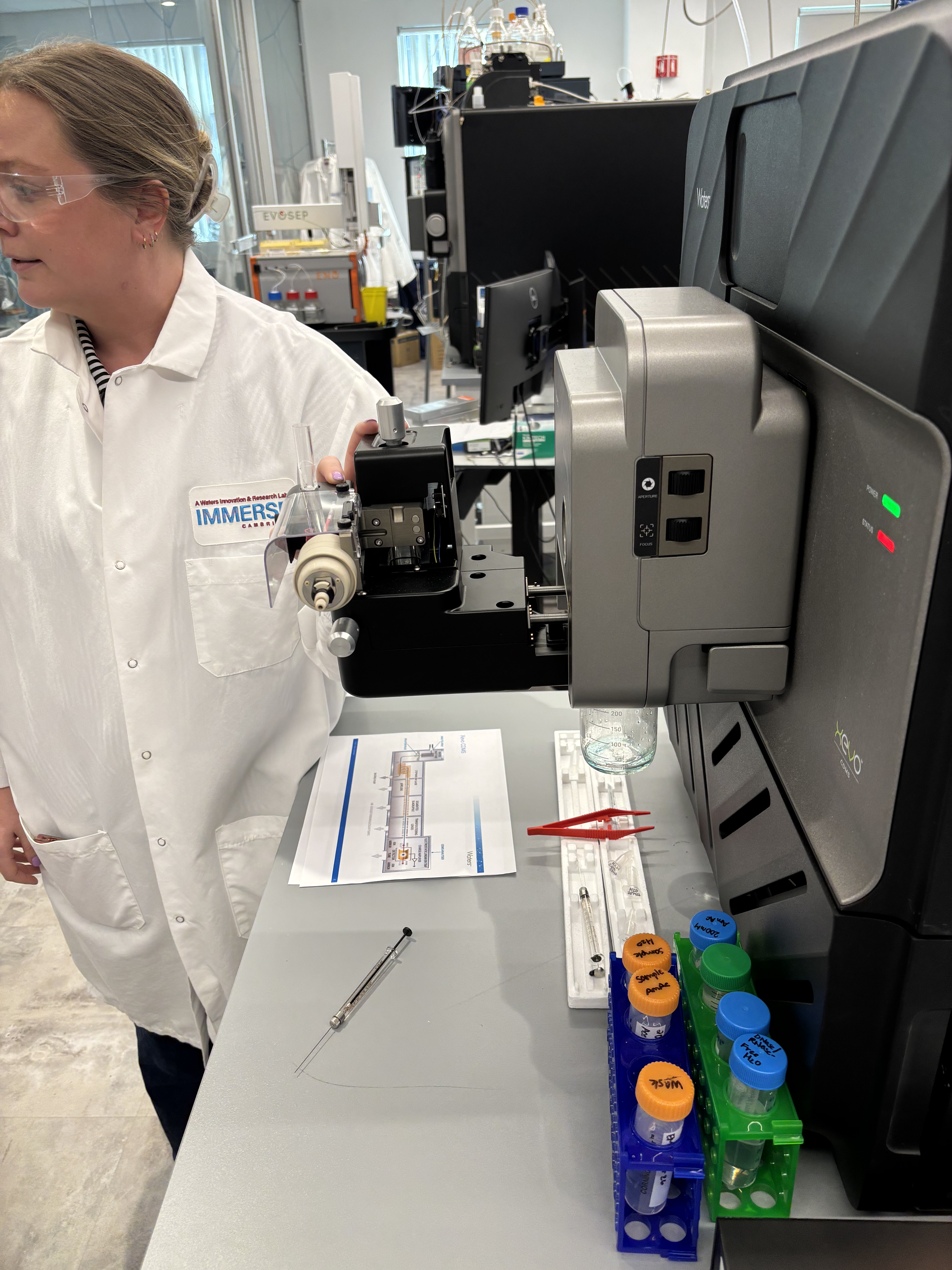
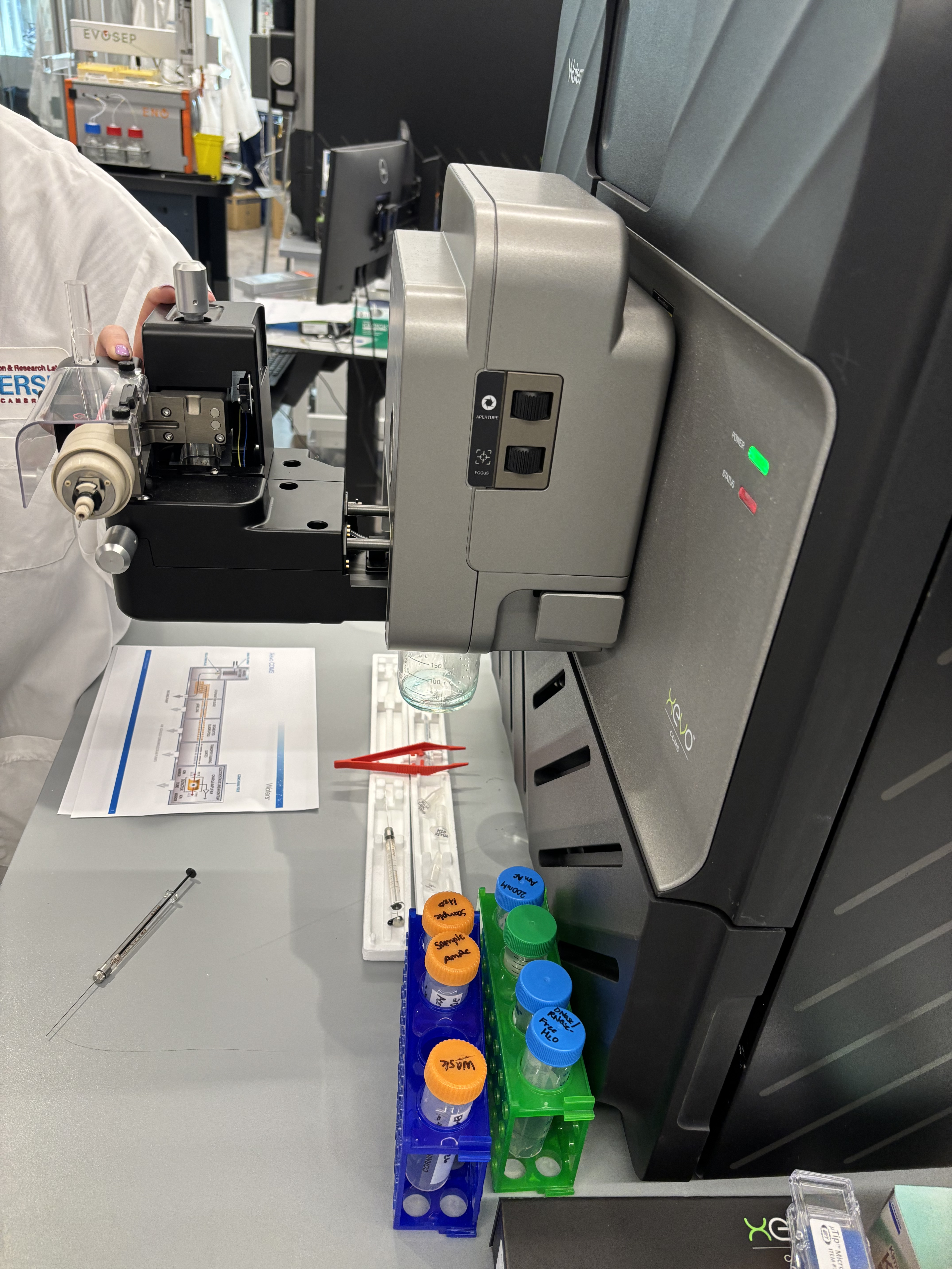
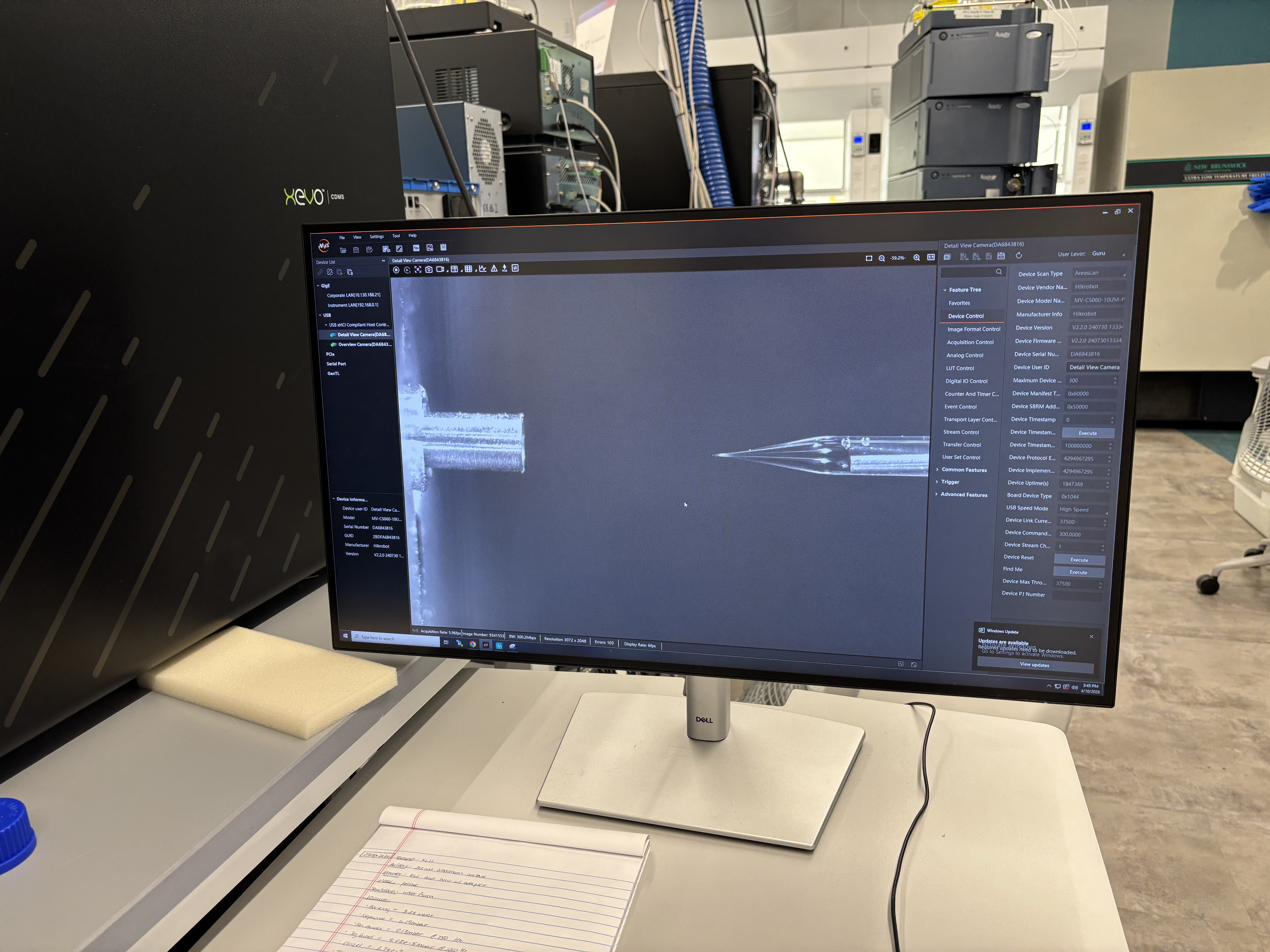
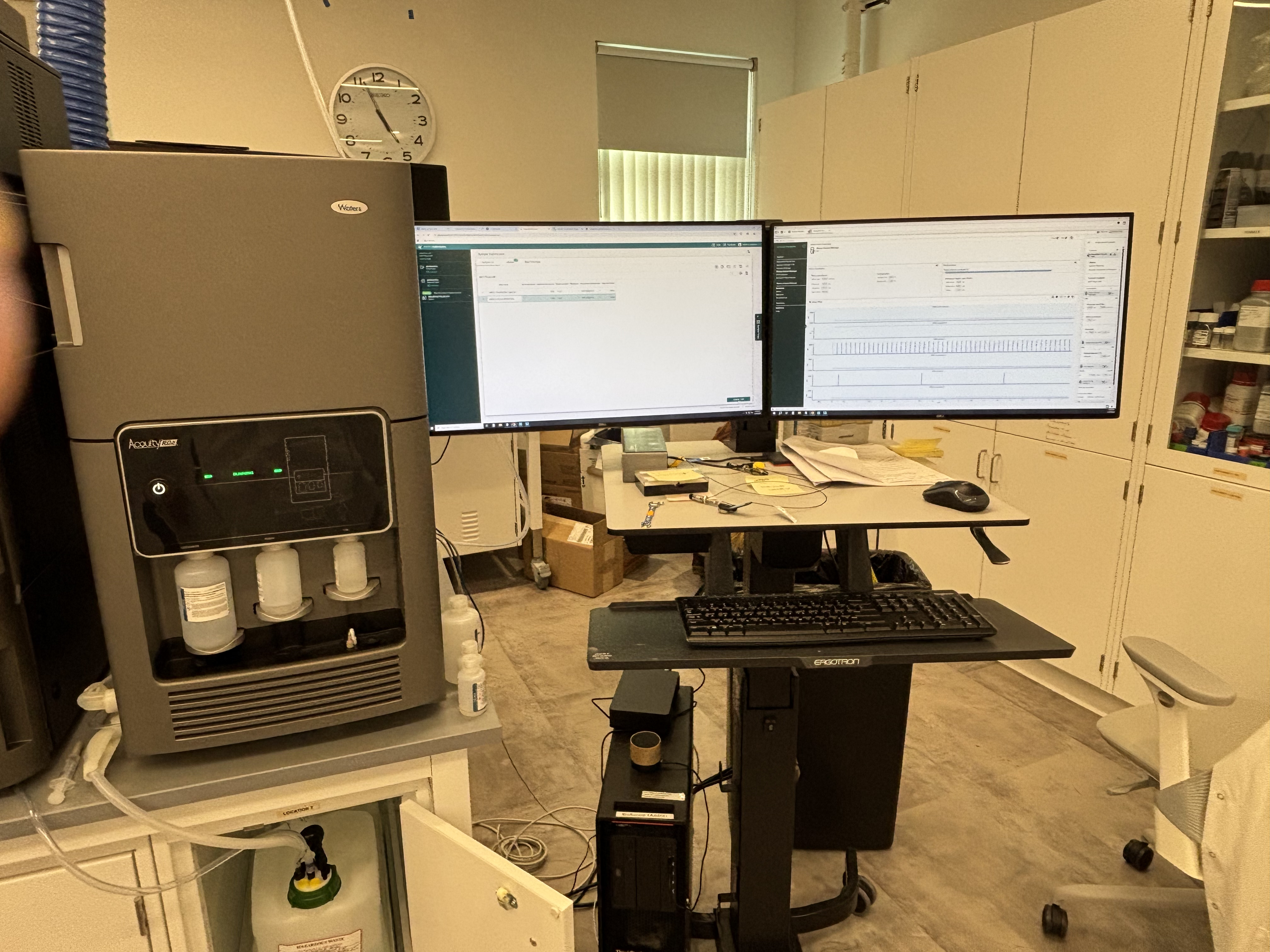
Photos
Lab Overview
This lab introduced us to mass spectrometry as a way to identify and measure molecules in a sample. The course page lists this as the Week 10 Mass Spectrometry lab, under the broader theme of advanced imaging and measurement technology.
The main idea of the lab was to understand the full measurement pipeline, not just the final spectrum. A sample has to be prepared, placed in the correct position, associated with the correct software method, run through the instrument, and then analyzed from the output data.
Protocol Understanding
The workflow started with organizing the samples and making sure each tube or vial corresponded to the correct entry in the software. This is a small but important part of the protocol because the instrument can run multiple samples automatically. If the physical sample position and the software sample list do not match, the data can be assigned to the wrong sample.
In a typical Waters LC-MS workflow, the sample is injected into a liquid chromatography system. The liquid solvent carries the sample through the column, where different molecules separate based on how they interact with the column material and solvent conditions. This means molecules do not all reach the mass spectrometer at the same time.
After separation, the sample enters the ionization source. The molecules are converted into ions so that they can be manipulated and detected by the mass spectrometer. The instrument then separates ions by mass-to-charge ratio, usually written as m/z. The detector records signals at different m/z values, producing peaks that can be viewed in the software.
What Was Done
In the lab, we observed the Waters instrument setup and how samples are prepared and loaded for analysis. The sample racks and tubes had to be organized carefully so that the correct sample was associated with the correct run. We also looked at the computer interface used to control the instrument and view the output.
The instrument method controls details such as the sample injection, run duration, solvent conditions, and detector settings. Once the run begins, the system automatically moves the sample through the measurement pipeline. The resulting data can include chromatograms, which show signal over time, and spectra, which show signal across mass-to-charge ratios.
Data Interpretation
The output of mass spectrometry is not a simple visual result like a colony plate or gel band. Instead, the result is a set of peaks. The position of a peak can help identify a molecule or fragment, while the intensity of the peak gives information about how strong that signal is.
A key thing I learned is that mass spectrometry data requires interpretation. Some peaks may correspond to the molecule of interest, while others can come from fragments, contaminants, solvent, background signal, or noise. This makes the software and analysis step a core part of the protocol.
Reflection
This lab helped me understand mass spectrometry as a bridge between wet-lab sample handling and computational analysis. The physical work involves preparing, labeling, and loading samples, but the final result depends on interpreting instrument data.
The most useful part was seeing the complete pipeline. The instrument can produce very precise measurements, but the quality of the result still depends on good sample organization, correct method setup, and careful interpretation. Even though I did not independently operate the full instrument myself, this lab made the role of mass spectrometry much clearer. It is useful when we need detailed information about what molecules are present in a sample, rather than just whether an experiment visibly worked.
Week 1 Lab: Pipetting
Week 3 Lab
Dialga: A Legendary Pokemon from the Sinnoh region