title: ‘Week 1 HW: Principles & Practices’ weight: 10 Week 1 HW: Principles & Practices Introduction and Motivation This week emphasized that biological engineering is not only about what we can build, but also how and why we choose to build it. The lectures and recitation highlighted that ethics, safety, security, and governance should not be treated as external constraints applied only after a technology is developed. Instead, they should be considered as integral design dimensions from the earliest stages of a project.
Part 0 — Gel Electrophoresis Basics (Concepts) This week, I reviewed how gel electrophoresis turns a DNA “mixture” into an interpretable pattern. In an agarose gel, DNA fragments migrate toward the positive electrode because DNA is negatively charged, and smaller fragments travel farther through the gel matrix than larger ones. A DNA ladder provides a size reference so unknown bands can be estimated in base pairs. When a restriction enzyme digest is performed, the DNA sequence is converted into a predictable set of fragment lengths, and those fragments appear as bands at specific positions. Band brightness is roughly related to how much DNA mass is in that fragment (longer fragments can look brighter if molar amounts are similar). Overall, the key idea is that restriction digests plus gels let you “read out” a cutting pattern, validate identity, and compare designs or conditions in a simple visual way.
This week emphasized that biological engineering is not only about what we can build, but also how and why we choose to build it. The lectures and recitation highlighted that ethics, safety, security, and governance should not be treated as external constraints applied only after a technology is developed. Instead, they should be considered as integral design dimensions from the earliest stages of a project.
Revisiting a previous biosensing project through the HTGAA framework allowed me to explicitly articulate design decisions that were originally motivated by technical performance, but which also carry strong ethical, safety, and governance implications. This exercise helped me move beyond a purely technical evaluation and reflect more deeply on responsibility, context, accessibility, and downstream impact.
Class Assignment: Biological Engineering Application and Governance
Biological Engineering Application
The biological engineering application I focus on is a cell-free biosensor based on a Pb²⁺-specific DNAzyme coupled to CRISPR-Cas12a, designed for the ultrasensitive detection of lead in water.
Lead contamination represents a serious public health concern, with no safe threshold for chronic exposure. While analytical techniques such as ICP-MS or atomic absorption spectroscopy provide high sensitivity and specificity, they require centralized laboratories, specialized equipment, trained personnel, and relatively long processing times. This limits their accessibility for frequent, decentralized, or field-based monitoring.
Previous generations of biological sensors, including whole-cell bacterial biosensors, demonstrated the feasibility of biological detection. However, whole-cell systems can suffer from long response times, relatively high detection limits, regulatory barriers, and biosafety concerns related to the use of living genetically modified organisms.
In contrast, this project deliberately adopts a cell-free, in vitro architecture. The goal is to translate the presence of Pb²⁺ into a fluorescent signal in under one hour, while reducing biological containment risks. The proposed system combines:
A Pb²⁺-responsive DNAzyme as the recognition module.
A DNA trigger released or exposed upon Pb²⁺-dependent cleavage.
A CRISPR-Cas12a amplification module activated by the DNA trigger.
A fluorescent reporter cleaved by activated Cas12a to produce a measurable signal.
The motivation behind this application is to combine high sensitivity, portability, and safety by design, enabling environmental monitoring in settings where conventional laboratory infrastructure is unavailable, while minimizing biological risks.
Governance and Policy Goals
Reframing this project within the HTGAA framework led to the identification of several governance and policy goals that extend beyond technical performance.
Goal A — Prevent Harm and Misuse
The first goal is to ensure that the technology does not enable harmful applications or irresponsible deployment.
Specific sub-goals include:
Avoid enabling biological manipulation, propagation, or amplification of hazardous agents.
Prevent repurposing of the sensing platform for unintended or harmful biological activities.
Avoid creating a false sense of security through poorly validated field tests.
Ensure that results are interpreted responsibly and not used to make unsupported public health or environmental claims.
Goal B — Enhance Biosafety and Biosecurity
The second goal is to reduce the biological risks associated with biosensor development and deployment.
Specific sub-goals include:
Minimize risks associated with handling living organisms by using a fully cell-free system.
Reduce the likelihood of accidental environmental release or uncontrolled replication.
Design the system so that it cannot reproduce, evolve, or persist in the environment.
Encourage safe handling, storage, and disposal of biological and chemical reagents.
Goal C — Promote Constructive and Equitable Use
The third goal is to ensure that the technology is used for beneficial, accessible, and socially responsible environmental monitoring.
Specific sub-goals include:
Enable access to sensitive environmental monitoring tools without requiring advanced infrastructure.
Support public health and environmental decision-making rather than surveillance, coercive enforcement, or unsupported alarmism.
Make limitations, false positives, false negatives, and validation requirements clear to users.
Encourage deployment in collaboration with local communities, public health actors, and environmental agencies.
Governance Actions
Option 1 — Safe-by-Design, Cell-Free System Architecture
Purpose
Many biosensing platforms rely on living cells, which introduce biosafety, containment, and regulatory challenges. This project replaces whole-cell systems with a fully cell-free, non-replicative architecture.
The proposed change is to integrate safety directly into the technical design. Instead of relying only on downstream regulation or user behavior, the system itself is designed to reduce the likelihood of biological release, persistence, or replication.
Design
This approach is implemented directly by academic researchers during the design phase and can be reinforced by funding agencies, institutional biosafety committees, and educational programs that prioritize safe-by-design technologies.
Key design features include:
No living genetically modified organisms in the final detection reaction.
No self-replicating biological components.
In vitro CRISPR-Cas12a activity limited to reporter cleavage.
Clear separation between detection chemistry and any organismal engineering.
Assumptions
This option assumes that:
Eliminating living components significantly reduces biosafety risks.
Performance can be maintained or improved in vitro.
The major risks of the platform are related more to deployment, interpretation, and reagent handling than to biological propagation.
Users will understand that a cell-free system is safer, but not risk-free.
Risks of Failure and “Success”
Failure risk: The system may be less robust in complex environmental matrices, such as dirty water samples containing inhibitors, particulates, organic matter, or competing metal ions.
Success risk: A highly portable test could be deployed too broadly without adequate validation, leading to overconfidence in results or inappropriate decision-making based on preliminary measurements.
Option 2 — Transparent Documentation of Limitations and Failures
Purpose
Scientific reporting often emphasizes successful outcomes while underreporting failures, optimization dead ends, matrix effects, and ambiguous results. This option proposes transparent documentation of both successful and unsuccessful experimental steps.
The goal is to improve reproducibility, avoid overclaiming, and make ethical reflection part of the scientific record.
Design
This action can be implemented through:
Detailed lab records.
Public documentation on the HTGAA website.
Clear separation between simulated, preliminary, and experimentally validated results.
Explicit reporting of failed designs, negative controls, and troubleshooting.
Discussion of limitations and uncertainties.
This action is mainly implemented by researchers, students, instructors, and academic communities, but it can also be encouraged by journals, funders, and training programs.
Assumptions
This option assumes that:
Transparency improves reproducibility.
Reporting failures can help others avoid repeating the same mistakes.
Open documentation builds trust.
Students and early-stage researchers can document uncertainty without being penalized for not having a perfect final result.
Risks of Failure and “Success”
Failure risk: Documentation could become superficial or performative if researchers include generic statements without meaningful detail.
Success risk: Excessive documentation requirements could increase workload, especially for students and early-stage researchers, and could discourage experimentation if not balanced with practical expectations.
Option 3 — Context-Specific Deployment Guidelines
Purpose
Environmental biosensors may be deployed in diverse contexts with different ethical, social, legal, and public health implications. A test used for classroom demonstration is not equivalent to a test used for regulatory enforcement or public health decision-making.
This option proposes context-aware deployment guidelines that distinguish between:
Educational use.
Research use.
Preliminary environmental screening.
Public health monitoring.
Regulatory or legal decision-making.
Design
These guidelines would be developed by public health and environmental agencies in collaboration with researchers, local institutions, and community stakeholders.
A context-specific guideline could include:
Minimum validation requirements before field use.
Clear interpretation guidelines for positive and negative results.
Requirements for confirmatory testing with gold-standard methods.
Communication protocols for reporting contamination risks.
Ethical considerations for community-level environmental data.
Assumptions
This option assumes that:
Misuse risk depends strongly on deployment context.
Local institutions have the capacity to enforce or adapt guidelines.
Communities benefit from access to environmental information when it is communicated responsibly.
Preliminary tests should support, not replace, validated analytical methods.
Risks of Failure and “Success”
Failure risk: Guidelines may be inconsistently applied across regions, especially where regulatory infrastructure is weak.
Success risk: If guidelines become too restrictive or bureaucratic, they could delay deployment in high-need environments where accessible monitoring is urgently needed.
Scoring Matrix
Scoring key: 1 = strongest / most favorable alignment with the policy goal 2 = moderate alignment 3 = weakest / least favorable alignment n/a = not applicable
Policy Goal / Evaluation Criterion
Option 1: Cell-free safe-by-design
Option 2: Transparent documentation
Option 3: Context-specific deployment guidelines
Enhance biosecurity by preventing incidents
1
2
2
Enhance biosecurity by helping respond
2
1
1
Foster lab safety by preventing incidents
1
2
2
Foster lab safety by helping respond
2
1
2
Protect the environment by preventing incidents
2
2
1
Protect the environment by helping respond
2
1
1
Minimize costs and burdens to stakeholders
1
3
2
Feasibility
1
2
2
Not impede research
1
2
3
Promote constructive applications
1
1
2
Prioritization and Recommendation
Based on this analysis, the highest priority should be given to Option 1: safe-by-design, cell-free architecture, complemented by Option 2: transparent documentation of limitations and failures.
This combination embeds ethical and governance considerations directly into technical design and research practice, rather than relying only on downstream regulation. The cell-free architecture reduces the biological risks associated with living engineered organisms, while transparent documentation reduces the risk of overclaiming, improves reproducibility, and helps future users understand the true limits of the system.
This combined approach is particularly relevant for academic research institutions, teaching laboratories, and funding agencies, where early design choices strongly influence future applications. While these decisions may introduce additional development effort, they significantly enhance safety, trust, and long-term societal benefit.
Option 3, context-specific deployment guidelines, is also important, but I would prioritize it at a later stage, once the technical system has been experimentally validated. Deployment governance becomes especially relevant when moving from proof-of-concept research to real-world environmental monitoring.
The main trade-off is that stronger governance can slow deployment. However, for environmental health technologies, speed should not come at the cost of unreliable or poorly interpreted results. A portable lead biosensor should empower communities and researchers, but it should not replace validated confirmatory testing before major public health or regulatory decisions are made.
Weekly Reflection
A key insight from this week is that biosensing technologies are not ethically neutral, even when developed for public health or environmental protection. Portability and accessibility are usually framed as purely positive features, but they can also enable misuse, misinterpretation, or premature deployment if the social and regulatory context is not carefully considered.
Engaging with the recitation examples reinforced the importance of situating my project at the detection and prevention end of the biological intervention spectrum. My proposed system does not edit genomes, release organisms, or introduce engineered biological entities into the environment. However, it still carries ethical responsibilities related to data quality, communication, access, and interpretation.
This week shifted my perspective from asking only:
Can this work?
to also asking:
Should it work this way, under what conditions, and who could be affected by its use?
That mindset is especially important for biosensors intended for environmental monitoring, because the consequences of a result are not only technical. A positive lead detection result could influence public trust, community concern, regulatory response, and resource allocation. Therefore, responsible biosensor development must include validation, transparency, and careful communication from the beginning.
Documentation Practice
In alignment with the course emphasis on documentation, I am recording all in silico design steps, experimental iterations, failed conditions, and troubleshooting decisions. This documentation is intended to support reproducibility, collaborative learning, and ethical transparency.
For this project, I aim to make visible the full design journey rather than only the successful outcomes. This includes:
Conceptual design decisions.
Sequence design rationale.
Simulation and modeling steps.
Failed or uncertain design choices.
Limitations of the proposed detection system.
Safety and governance considerations.
This approach is important because reproducibility and responsible innovation depend not only on final results, but also on documenting how those results were reached.
Week 2 Lecture Preparation
In preparation for Week 2, “DNA Read, Write, and Edit,” I reviewed the lecture questions and answered the required prompts from Professor Jacobson, Dr. LeProust, and one selected question from Professor Church.
Professor Jacobson — Homework Questions
1. What is the error rate of polymerase? How does this compare to the length of the human genome? How does biology deal with that discrepancy?
DNA polymerases are highly accurate, but they are not perfect. A typical raw DNA polymerase error rate can be around 10-5 to 10-6 errors per nucleotide incorporated, depending on the polymerase and biological context. After proofreading and mismatch repair, the final replication error rate can be reduced to approximately 10-9 to 10-10 errors per base per cell division.
This is important because the human genome contains approximately 3.2 billion base pairs in the haploid genome, or about 6.4 billion base pairs in a diploid cell. Even a very low error rate can therefore generate many potential mistakes if no correction mechanisms exist.
Biology deals with this discrepancy through several layers of quality control:
Nucleotide selectivity by DNA polymerases.
Exonuclease proofreading, which removes incorrectly incorporated nucleotides.
Mismatch repair, which corrects errors that escape proofreading.
DNA damage repair pathways, which repair chemically damaged bases or strand breaks.
Cell-cycle checkpoints, which prevent damaged cells from continuing division.
Apoptosis or senescence, which can eliminate cells with severe genome instability.
Together, these mechanisms reduce the mutational burden and help preserve genome integrity across cell divisions.
2. How many different ways are there to code for an average human protein? In practice, what are some of the reasons that all of these different codes do not work to code for the protein of interest?
Because the genetic code is degenerate, most amino acids can be encoded by more than one codon. For a protein of length n, the number of possible DNA coding sequences is the product of the number of synonymous codons available for each amino acid:
Number of possible coding sequences = d1 × d2 × d3 × ... × dn
where each d is the codon degeneracy for a given amino acid.
For an average human protein of several hundred amino acids, this number is astronomically large. A rough estimate using an average degeneracy of about 3 codons per amino acid for a 400-amino-acid protein gives:
3^400 ≈ 10^190 possible coding sequences
However, not all synonymous coding sequences work equally well in practice. Several factors influence whether a DNA sequence can efficiently produce the desired protein:
Codon usage bias: Different organisms prefer different synonymous codons.
tRNA abundance: Rare codons can slow translation or reduce expression.
GC content: Very high or very low GC content can affect synthesis, stability, and amplification.
mRNA secondary structure: Strong structures near the ribosome binding site or start codon can reduce translation.
Cryptic splice sites: In eukaryotic systems, some sequences may be incorrectly spliced.
Premature termination or polyadenylation-like motifs: These can interfere with transcription or RNA processing.
Internal repeats: Repetitive DNA can be difficult to synthesize, clone, or maintain.
Restriction sites: Some sequences may contain sites that interfere with cloning strategies.
RNA stability: Synonymous changes can alter mRNA half-life.
Translation speed and co-translational folding: Codon choice can influence how the protein folds during translation.
Synthesis and assembly constraints: Some DNA sequences are harder to chemically synthesize or assemble.
Therefore, although the theoretical number of coding sequences is enormous, the number of practical, expressible, and functional sequences is much smaller.
Dr. LeProust — Homework Questions
1. What is the most commonly used method for oligo synthesis currently?
The most commonly used method for oligonucleotide synthesis is solid-phase phosphoramidite chemistry.
In this method, the oligonucleotide is synthesized step by step on a solid support. Each nucleotide addition cycle typically includes:
Deprotection, which exposes a reactive hydroxyl group.
Coupling, where the next phosphoramidite nucleotide is added.
Capping, which blocks unreacted chains.
Oxidation, which stabilizes the phosphate linkage.
This cyclic chemistry allows controlled synthesis of DNA or RNA oligonucleotides with defined sequences.
2. Why is it difficult to make oligos longer than 200 nt via direct synthesis?
It is difficult to synthesize oligos longer than approximately 200 nucleotides because oligo synthesis is a stepwise chemical process and each coupling cycle is less than 100% efficient.
Even if each individual step is highly efficient, small inefficiencies accumulate over many cycles. As the sequence becomes longer, several problems increase:
The fraction of full-length correct product decreases.
Truncated products accumulate.
Deletion errors become more likely.
Depurination and chemical damage can occur.
Sequence heterogeneity increases.
Purification becomes more difficult.
Quality control becomes more challenging.
For example, if each coupling step were 99% efficient, the theoretical full-length yield after 200 additions would be much lower than after 50 additions. Therefore, long oligos are harder to synthesize accurately and economically by direct chemical synthesis.
3. Why can’t you make a 2000 bp gene via direct oligo synthesis?
A 2000 bp gene cannot be reliably produced by direct oligo synthesis because the cumulative error rate and loss of full-length product over thousands of synthesis cycles would be too high.
Directly synthesizing a 2000 nucleotide sequence would produce a complex mixture of incomplete, mutated, and damaged products rather than a clean full-length gene. The longer the sequence, the lower the probability that every nucleotide was added correctly.
Instead, genes are usually produced by a modular strategy:
Shorter oligos are chemically synthesized.
These oligos are assembled into larger fragments.
Larger fragments are joined enzymatically or through DNA assembly methods.
The final construct is cloned and sequence-verified.
This strategy improves yield, accuracy, and error correction. It also allows problematic regions to be redesigned or corrected before the final full-length gene is obtained.
George Church — Homework Question
Question chosen
AA:AA and NA:NA codes — What code would you suggest for AA:AA interactions?
Why We Need a Code and What It Can and Cannot Do
Protein-protein interactions are not “pairwise letters” like Watson-Crick base pairing. They depend strongly on three-dimensional context, including distance, orientation, solvent exposure, dynamics, post-translational modifications, pH, ionic strength, and local environment.
Still, a useful amino acid to amino acid interaction “code” can exist as a coarse-grained interaction alphabet: a compact way to describe which residue pairs are likely to attract, repel, stabilize, or modulate protein interfaces.
The goal is not to create a perfect predictor of protein structure. Instead, the goal is to create a portable interaction language that is:
Symmetric: A-B is equivalent to B-A.
Composable: Many local contacts can describe one interface.
Extendable: The code can include non-standard amino acids or post-translational modifications.
Human-usable: The system should be simpler than a full 20 × 20 interaction table.
Proposed AA:AA Interaction Code
I propose a two-layer code.
Layer 1 — Assign Each Amino Acid to an Interaction Class
Each amino acid can be assigned to a dominant chemical interaction class:
Class
Meaning
Amino acids
H
Hydrophobic aliphatic
A, V, L, I, M
Ar
Aromatic
F, Y, W
P
Polar uncharged
S, T, N, Q
D+
Cationic / donor-leaning
K, R, H
A−
Acidic / anionic
D, E
S
Sulfur / thiol special
C
G
Glycine / conformational special
G
Pro
Proline / conformational breaker
P
H and Ar are separated because aromatic residues can participate in π-stacking and cation-π interactions, which are distinct from simple hydrophobic packing. Cysteine is treated separately because it can form disulfide bonds and participate in redox or metal-binding interactions. Glycine and proline are treated separately because their main importance is often conformational rather than purely chemical.
Layer 2 — Use an Interaction Operator Between Classes
A small set of operators can describe the type of contact between classes:
Operator
Meaning
Example
⊕
Favorable hydrophobic packing
H-H, H-Ar, Ar-Ar
±
Electrostatic attraction / salt bridge
D+ - A−
≠
Electrostatic repulsion
D+ - D+ or A− - A−
⋯
Hydrogen bonding
P-P, P-D+, P-A−
π+
Cation-π interaction
D+ - Ar
S-S
Disulfide bond
Cys-Cys
⟂
Conformational modulation
Pro-X or Gly-X
This yields a compact grammar:
Contact = Class(residue 1) OP Class(residue 2)
Examples:
Lys-Glu → D+ ± A−
Leu-Ile → H ⊕ H
Arg-Trp → D+ π+ Ar
Cys-Cys → S-S
Pro-X → Pro ⟂ X
Why This Code Is Useful
This code is useful because it compresses many possible amino acid interactions into a smaller, interpretable set of interaction modes.
Advantages include:
Small alphabet, broad coverage: It reduces the complexity of 20 × 20 amino acid combinations into a readable set of chemical interaction types.
Extendability: It can be expanded to include modified residues or non-standard amino acids.
Connection to protein design: Protein interface design often relies on the same basic principles: hydrophobic cores, hydrogen bond networks, salt bridges, cation-π interactions, disulfides, and conformational constraints.
Interpretability: It provides a human-readable vocabulary for reasoning about protein-protein interfaces.
Known Limitations
This code has important limitations:
Context dependence: The same residue pair can behave differently depending on whether it is buried or solvent-exposed.
pH dependence: Protonation states can change interactions, especially for histidine, acidic residues, and termini.
Geometry dependence: A chemically favorable interaction may not occur if the residues are not properly oriented.
Water mediation: Some contacts are mediated by water molecules rather than direct side-chain interactions.
Many-body effects: Protein interfaces are cooperative networks, not just sums of pairwise contacts.
Not a folding code: This is an interaction vocabulary, not a complete structural prediction system.
Optional Refinement
If more precision is needed, an environmental tag can be added:
(B) = buried
(E) = exposed
For example:
D+ ± A− (B)
This would represent a buried salt bridge, which may have a different energetic contribution than an exposed salt bridge.
Similarly:
H ⊕ H (B)
would represent buried hydrophobic packing, which is usually more stabilizing than exposed hydrophobic contact.
AI / Prompt Citation
I used ChatGPT to help draft and structure this answer.
Prompt used:
Given George Church’s lecture framing of codes beyond DNA-to-amino-acid translation, propose a concise, extensible AA:AA interaction code that captures major interaction types including hydrophobic contacts, salt bridges, hydrogen bonds, cation-π interactions, disulfides, and conformational effects.
I then edited and adapted the response to fit my own reasoning and the context of this homework.
Lab Preparation Note
The lab preparation and MIT safety training components were listed as required for MIT/Harvard students, but not applicable to Committed Listeners. Therefore, I did not complete the in-person lab-specific safety training or Atlas safety modules as part of this homework.
Summary
This week helped establish a framework for thinking about biological engineering as a technical, ethical, and governance challenge. For my proposed DNAzyme-Cas12a Pb²⁺ biosensor, the most important lesson was that safety and responsibility should be designed into the system from the beginning.
The main governance strategy I would prioritize is a safe-by-design, cell-free architecture, combined with transparent documentation of limitations, failures, and uncertainties. This combination supports biosafety, reproducibility, and constructive use while preserving the educational and scientific value of the project.
Week 2 HW: DNA Read, Write, & Edit
Part 0 — Gel Electrophoresis Basics (Concepts)
This week, I reviewed how gel electrophoresis turns a DNA “mixture” into an interpretable pattern. In an agarose gel, DNA fragments migrate toward the positive electrode because DNA is negatively charged, and smaller fragments travel farther through the gel matrix than larger ones. A DNA ladder provides a size reference so unknown bands can be estimated in base pairs. When a restriction enzyme digest is performed, the DNA sequence is converted into a predictable set of fragment lengths, and those fragments appear as bands at specific positions. Band brightness is roughly related to how much DNA mass is in that fragment (longer fragments can look brighter if molar amounts are similar). Overall, the key idea is that restriction digests plus gels let you “read out” a cutting pattern, validate identity, and compare designs or conditions in a simple visual way.
I created a “gel art” pattern inspired by the idea that restriction digests can produce recognizable visual signatures. The design uses symmetry and band density as the main visual elements: enzymes with few cuts generate sparse lanes (lighter), while enzymes with many cuts generate dense lanes (darker).
Lane plan (left → right): Ladder (Life 1 kb Plus), ApaI, EcoRI, HaeIII, EcoRI, ApaI.
HaeIII creates a high-density fragmentation pattern that acts as the “dark center,” while EcoRI and ApaI provide low-cut, high-molecular-weight bands that frame the pattern.
Part 3 — DNA Design Challenge
3.1 Protein choice
I chose sfGFP (superfolder GFP) as the target protein because it is a robust fluorescent reporter widely used to validate expression, folding, and cloning workflows. It provides an easy quantitative readout (fluorescence) and is a standard “sanity check” part in many synthetic biology builds.
3.2 Reverse translation (baseline CDS)
Starting from the sfGFP amino-acid sequence, I generated a DNA coding sequence (CDS) by back-translation using a codon-usage–matching approach (Benchling output). This produces a valid CDS encoding the same protein sequence.
Protein length: 246 aa
DNA CDS length (no stop codon): 738 bp
sfGFP amino-acid sequence (246 aa):

MSKGEELFTGVVPILVELDGDVNGHKFSVRGEGEGDATNGKLTLKFICTTGKLPVPWPTL
VTTLTYGVQCFSRYPDHMKRHDFFKSAMPEGYVQERTISFKDDGTYKTRAEVKFEGDTLV
NRIELKGIDFKEDGNILGHKLEYNFNSHNVYITADKQKNGIKANFKIRHNVEDGSVQLAD
HYQQNTPIGDGPVLLPDNHYLSTQSVLSKDPNEKRDHMVLLEFVTAAGITHGMDELYKGS
HHHHHH


Back-translated / codon-usage–matched CDS (low GC target):
ATGTCAAAAGGTGAGGAATTATTTACCGGAGTAGTACCAATACTGGTAGAATTAGATGGCG
ATGTTAATGGGCATAAGTTTTCAGTGCGTGGAGAAGGAGAAGGCGATGCTACAAATGGAAA
ATTAACGTTAAAATTTATTTGTACTACTGGGAAACTACCTGTACCTTGGCCAACTTTAGTT
ACAACCTTAACATATGGTGTACAATGTTTTTCTCGTTATCCAGATCATATGAAACGTCATG
ATTTTTTTAAAAGTGCGATGCCTGAAGGTTACGTTCAAGAAAGAACTATATCTTTTAAAGAT
GATGGTACATATAAAACACGAGCTGAAGTAAAATTTGAAGGTGATACTTTGGTTAATAGAAT
TGAACTTAAAGGGATTGATTTTAAGGAAGATGGAAATATTCTCGGACACAAATTAGAATACA
ATTTTAATTCACATAATGTTTACATAACAGCTGATAAACAAAAAAATGGCATAAAAGCAAAT
TTTAAAATAAGACATAATGTAGAAGATGGAAGTGTCCAATTAGCAGATCATTATCAGCAAAA
CACACCAATTGGTGATGGTCCTGTCCTTTTACCAGATAATCATTATTTATCAACCCAATCTG
TTTTGTCAAAAGATCCGAATGAAAAAAGAGATCATATGGTTTTATTGGAATTTGTAACAGCA
GCAGGTATTACTCATGGCATGGATGAATTATATAAAGGCTCTCATCATCATCATCATCAT
Codon optimization for E. coli
I then codon-optimized the CDS for Escherichia coli using a “use best codon” strategy. As expected, the amino-acid sequence is unchanged, but the nucleotide sequence changes due to synonymous codon choices that better match E. coli translation preferences.
Nucleotide identity (baseline vs optimized): 76.96%
GC content (baseline, codon-usage–matched): 33.0%
GC content (optimized, best-codon): 50.0%
Rare codons: 11 (baseline) vs 0 (optimized)
Hairpins (reported by the tool): 0 in both
Thymine fraction (reported by the tool): 0.30 (baseline) vs 0.21 (optimized)
ATGAGCAAAGGCGAAGAACTGTTTACCGGCGTGGTGCCGATTCTGGTGGAACTGGATGGCGAT
GTGAACGGCCATAAATTTAGCGTGCGCGGCGAAGGCGAAGGCGATGCGACCAACGGCAAACT
GACCCTGAAATTTATTTGCACCACCGGCAAACTGCCGGTGCCGTGGCCGACCCTGGTGACCA
CCCTGACCTATGGCGTGCAGTGCTTTAGCCGCTATCCGGATCATATGAAACGCCATGATTTT
TTTAAAAGCGCGATGCCGGAAGGCTATGTGCAGGAACGCACCATTAGCTTTAAAGATGATGG
CACCTATAAAACCCGCGCGGAAGTGAAATTTGAAGGCGATACCCTGGTGAACCGCATTGAAC
TGAAAGGCATTGATTTTAAAGAAGATGGCAACATTCTGGGCCATAAACTGGAATATAACTTT
AACAGCCATAACGTGTATATTACCGCGGATAAACAGAAAAACGGCATTAAAGCGAACTTTAA
AATTCGCCATAACGTGGAAGATGGCAGCGTGCAGCTGGCGGATCATTATCAGCAGAACACCC
CGATTGGCGATGGCCCGGTGCTGCTGCCGGATAACCATTATCTGAGCACCCAGAGCGTGCTG
AGCAAAGATCCGAACGAAAAACGCGATCATATGGTGCTGCTGGAATTTGTGACCGCGGCGGGC
ATTACCCATGGCATGGATGAACTGTATAAAGGCAGCCATCATCATCATCATCATCAT
Best way to obtain the DNA
For a ~0.74 kb CDS like sfGFP, the most straightforward approach is gene synthesis (ordering a dsDNA fragment). It is fast, accurate, and does not require an existing template. If a plasmid template is already available, an alternative is PCR amplification + cloning (e.g., restriction cloning or Gibson), but synthesis avoids PCR-introduced mutations and simplifies the workflow.
Codon-optimized CDS (best codons, medium GC target)
## Part 4 — DNA Write (Ordering + Construct Design)
### 4.1 Expression cassette design (what I would build)
To express **sfGFP in *E. coli***, I would build a standard bacterial expression cassette:
- **Promoter:** T7 promoter (for high expression in BL21(DE3)-like strains) or a strong constitutive promoter if T7 is not desired
- **RBS:** strong bacterial RBS (e.g., a consensus Shine–Dalgarno / gene10-like RBS)
- **CDS:** sfGFP coding sequence, codon-optimized for *E. coli* (AA sequence unchanged)
- **Tag / stop:** optional **C-terminal 6xHis** tag for purification + **stop codon**
- **Terminator:** strong transcription terminator (e.g., T7 terminator / bacterial terminator)
This design is simple, robust, and makes fluorescence an immediate readout for “does expression work?”.
### 4.2 What I would order (DNA “write” step)
Because the sfGFP CDS is short (~0.7–0.8 kb), the most straightforward approach is **DNA synthesis** (a dsDNA fragment or a cloned gene). Concretely, I would order one of these:
**Option A — Gene fragment (fast + flexible)**
- Order the **sfGFP insert as dsDNA** with flanking overlaps for Gibson/HiFi assembly (or with restriction sites).
- Then clone into an expression plasmid in the lab.
**Option B — Cloned gene in a plasmid (one-step ready)**
- Order **sfGFP already cloned** into a high-copy plasmid backbone.
### 4.3 Twist Bioscience access limitation (Argentina) + workaround plan
From my location (Argentina), the Twist ordering portal is not accessible and prompts me to contact a local operator. In a real order scenario, I would do one of the following:

1) **Contact Twist local sales/support** (as requested) and place the order via email (sequence + vector + cloning format).
2) Use an **alternative synthesis provider** that ships to my region (e.g., ordering a dsDNA fragment from another vendor) and then perform the same assembly into an equivalent plasmid backbone.
For the purposes of this homework, I describe the intended order and construct as if placing a standard synthesis + cloning order.
### 4.4 Vector choice and final construct
If using Twist’s catalog, I would choose a standard **high-copy AmpR plasmid backbone** (e.g., a pTwist Amp high-copy–type vector), and insert the sfGFP expression cassette into it.
Final construct conceptually looks like:
**[T7 promoter] – [RBS] – [sfGFP CDS (E. coli optimized)] – [6xHis] – [STOP] – [Terminator]**
### 4.5 How I would obtain protein from this DNA (high-level workflow)
1) **Assemble** the insert into the plasmid (Gibson/HiFi or restriction cloning).
2) **Transform** into *E. coli* (expression strain if using T7).
3) **Verify** by sequencing (to confirm sfGFP is correct and in-frame).
4) **Express** and measure fluorescence as a fast functional readout.
5) (Optional) **Purify** via His-tag if purification is required.
This approach separates “DNA write” (ordering/synthesis) from “DNA read” (sequencing verification) and “DNA function” (fluorescence output).
## Part 5 — DNA Read / Write / Edit (Dengue focus: Argentina)
### 5.1 DNA Read
**(i) What DNA/RNA would I want to sequence and why?**
I would focus on **genomic surveillance of Dengue virus (DENV) in Argentina**, integrating **clinical** and **environmental** sequencing to support public health decisions in real time.
Concretely, I would sequence:
1) **Clinical DENV genomes (RNA → cDNA)** from a **representative subset** of confirmed cases:
- **Across regions** (e.g., AMBA vs. northern provinces where dengue burden can be higher).
- **Across time** (weekly/biweekly sampling during season peaks).
- **Across epidemiological contexts** (outbreak clusters, travel-associated cases, and sporadic detections).
**Why:**
- To track **serotype dynamics** (DENV-1/2/3/4) and detect shifts that may correlate with outbreak intensity.
- To monitor **lineage introductions** (new clades entering a province) and infer **transmission connectivity** between regions.
- To support **molecular epidemiology**: identify clusters, potential superspreading contexts, and genomic signatures associated with rapid spread (without overclaiming causality).
- To generate local datasets that strengthen **regional capacity** and reduce dependence on external sequencing pipelines.
2) **Environmental DENV surveillance in Aedes aegypti pools** (and optionally wastewater as exploratory):
- **Mosquito pools** (RT-PCR confirmed) from vector surveillance programs: this can provide early hints of circulating serotypes/lineages even before clinical case counts surge.
- **Wastewater** is less standard for DENV than for enteric viruses, but could be explored as a research add-on; vector-based sampling is usually more direct for arboviruses.
**Why:**
- To get **earlier warning signals** and a broader picture of circulation beyond who shows up at clinics.
- To link **vector circulation** with **human cases**, improving outbreak models.
---
**(ii) What sequencing technology would I use and why?**
I would use a **two-tier strategy**:
- **Illumina short-read sequencing (2nd generation)** for routine surveillance:
- High per-base accuracy, scalable multiplexing, strong variant calling.
- Great for producing reliable consensus genomes and phylogenies.
- **Oxford Nanopore sequencing (3rd generation)** for rapid, field-forward situations:
- Faster turnaround when you need same-week answers (e.g., suspected new introduction or unusual outbreak).
- Useful for decentralized labs or mobile workflows, at the cost of higher raw read error (mitigated by coverage + consensus polishing).
This hybrid approach fits a realistic public health workflow: Illumina as the “gold standard backbone”, Nanopore as the “rapid response tool”.
---
**1) Is it first-, second-, or third-generation? How so?**
- **Illumina = second-generation**: massively parallel short reads (sequencing-by-synthesis).
- **Nanopore = third-generation**: single-molecule sequencing, long reads, electrical signal through nanopores.
---
**2) What is the input? How do you prepare your input? Essential steps.**
**Input:** Dengue is an **RNA virus**, so the primary input is **viral RNA** extracted from samples, then converted to **cDNA**.
A practical pipeline:
**Clinical samples (serum/plasma/whole blood, depending on stage):**
1. **Sample + metadata collection** (date, location, Ct value, suspected serotype if known, etc.).
2. **RNA extraction**.
3. **RT step → cDNA**.
4. **Target enrichment strategy** (choose one):
- **Amplicon tiling PCR** (common for viral genomes; efficient and cheap).
- OR **capture-based enrichment** (more flexible but more expensive).
5. **Library preparation**:
- Illumina: adapter ligation + indexes (multiplexing), optional PCR.
- Nanopore: end-repair + adapter ligation, optional barcoding.
6. **Sequencing run**.
7. **Bioinformatics**: QC → mapping → consensus → variants → phylogeny.
**Mosquito pool samples:**
1. **Pool preparation** (Aedes aegypti pools, ideally with RT-qPCR confirmation).
2. **RNA extraction** (often with inhibitors → extra QC).
3. RT → cDNA, then same as above.
**Key practical note:** For DENV, sampling time matters: early infection tends to have higher viremia (better genome recovery). Also, using Ct thresholds to select samples improves success rate.
---
**3) How does it decode the bases (base calling)?**
- **Illumina**: fluorescent signals from nucleotide incorporation per cycle → base calls + quality scores.
- **Nanopore**: ionic current shifts as molecules pass through the pore → signal-to-sequence base calling (model-based), then consensus polishing.
---
**4) What is the output?**
- **FASTQ** reads (with quality scores).
- **BAM/CRAM** alignments to a reference genome.
- **Consensus genome FASTA** per sample.
- **Variant calls (VCF)** (when appropriate).
- **QC reports** (coverage depth, % genome recovered, contamination checks).
- Downstream: **phylogenetic trees** and **lineage/cluster summaries** for epidemiological interpretation.
---
### 5.2 DNA Write
**(i) What DNA would I want to synthesize and why? (Dengue-focused)**
I would “write” DNA that enables **faster and more deployable dengue diagnostics** and/or supports local R&D.
Three concrete synthesis targets:
1) **DENV diagnostic standards and controls** (safe, non-infectious):
- Synthetic **gene fragments** (e.g., conserved regions of DENV genome used in RT-qPCR/CRISPR assays).
- **Positive control templates** for assay development and QA/QC.
**Why:** robust controls are crucial for reliable diagnostics, especially across multiple labs and seasons.
2) **CRISPR-based dengue detection components** (research prototype):
- Synthetic DNA templates to generate **RNA targets** (IVT) or **reporter constructs** for assay benchmarking.
- If building cell-free or isothermal detection workflows, you can synthesize the necessary templates without needing infectious material.
**Why:** safer, faster iteration.
3) **Aedes-related biosensor modules** (optional):
- DNA parts for sensor chassis optimization (e.g., expression cassettes for reporters in E. coli cell-free systems).
**Why:** create modular “plug-and-play” parts to accelerate prototyping.
---
**(ii) What technology would I use for DNA synthesis and why?**
- For ~0.3–3 kb fragments: **commercial gene synthesis** (dsDNA fragments or cloned gene in a plasmid).
- For many variants: **oligo pools** (array-based synthesis) + assembly.
**Why:** speed + reliability, avoids PCR errors, and supports rapid iteration (especially when you want multiple versions: different primers, target regions, or assay designs).
---
**1) Essential steps (high-level)**
- Design sequence (include constraints: avoid repeats/extreme GC, include needed cloning sites/overlaps).
- Order as dsDNA fragment (or oligos + assembly).
- If needed: clone into plasmid backbone (Gibson/HiFi or restriction cloning).
- Verify by sequencing (at least Sanger for inserts, or NGS for pools).
- Use as template/control in downstream assays.
---
**2) Limitations (speed, accuracy, scalability)**
- **Length & complexity**: longer sequences or high repeat content may fail or take longer.
- **Error rate**: increases with length; sometimes error correction or clone screening is needed.
- **Sequence constraints**: extreme GC, hairpins, homopolymers can reduce success.
- **Regulatory/shipping**: international access can be limited; some vendors require regional sales contact.
- **Cost**: scales with length and number of variants.
---
### 5.3 DNA Edit
**(i) What DNA would I want to edit and why? (Dengue context)**
I would focus on edits that are **ethically appropriate, feasible, and beneficial**, avoiding speculative or high-risk human germline scenarios.
Two realistic editing directions:
1) **Editing lab strains (E. coli or cell-free chassis) to improve dengue diagnostic prototyping**
Examples (conceptual):
- Reduce background nuclease activity that can degrade reporters.
- Improve expression stability of reporter proteins or enzymes used in readouts.
**Why:** more robust, reproducible diagnostics and faster prototyping cycles.
2) **Vector biology research (Aedes aegypti) — in controlled research settings**
Examples (high-level):
- Knock-in/knock-out genes to study **vector competence** or immune pathways relevant to arbovirus replication.
**Why:** better understanding of transmission biology can support long-term control strategies (with strong oversight and biosafety/ethics review).
---
**(ii) What technology would I use and why?**
- **CRISPR-Cas9** for knock-outs and knock-ins in model systems.
- **Base editing** for precise point mutations (when you want to avoid double-strand breaks).
- **Prime editing** for flexible small edits (insertions/deletions/substitutions) with less HDR dependence.
Choice depends on the edit:
- Big insertions → Cas9 + HDR (or targeted integration strategies).
- Single base changes → base editor.
- Small flexible edits → prime editor.
---
**1) How does it edit DNA? (conceptual steps)**
- Guide RNA targets a specific locus.
- Editor performs cut or base conversion.
- Cellular repair/processing results in the desired change.
- Screen and validate clones/lines.
---
**2) What preparation is needed and what is the input?**
- Target selection + guide design + off-target risk assessment.
- Editor delivery strategy (plasmid, mRNA, RNP).
- Optional donor template for HDR edits.
- Validation plan:
- PCR across the locus, Sanger/NGS confirmation,
- phenotype/functional assay relevant to the edit,
- off-target screening where appropriate.
---
**3) Limitations (efficiency/precision)**
- **Delivery** limitations (some cell types/organisms are difficult).
- **Off-targets** and unintended edits (varies with editor/guide).
- **HDR efficiency** can be low; requires careful design and screening.
- Need for **strong controls**, replication, and transparent reporting.
Week 3 HW: Lab Automation
## What I built
I created a two-color agar-art pattern (hummingbird) using the Automation Art Interface to generate coordinate lists for red and green dots. I then implemented an Opentrons OT-2 protocol (Python API) that dispenses 1 µL droplets at each (x, y) coordinate on a black agar plate.
Key constraints and design choices
Units: all coordinates are in mm.
Safety boundary: all points are constrained within a 40 mm radius from (0,0).
Droplet volume: 1 µL per dot (default for black agar plates).
Anti-streaking: used dispense_and_detach() motions to reduce streaking artifacts.
Contamination control: used one tip per color (red tip, green tip).
Efficiency: aspirated in chunks (up to 20 µL for P20) to reduce overhead while avoiding waste.
How I validated
I ran the provided Colab simulation and confirmed the visualized plate matches the intended design.
I confirmed the protocol does not raise any “outside radius” errors.
Simulator screenshot is saved in assets/simulation.png.
Files
protocol.py — OT-2 run code (robot-run block)
post_lab.md — mandatory post-lab questions (automation plan + paper summary)
weekly_questions.md — questions + short answers for node presentation
ai_disclosure.md — brief disclosure of AI assistance (if applicable)
pass this e.g. ‘Red’ and get back a Location which can be passed to aspirate()
def location_of_color(color_string):
for well,color in well_colors.items():
if color.lower() == color_string.lower():
return color_plate[well]
raise ValueError(f"No well found with color {color_string}")
For this lab, instead of calling pipette.dispense(1, loc) use this: dispense_and_detach(pipette, 1, loc)
def dispense_and_detach(pipette, volume, location):
"""
Move laterally 5mm above the plate (to avoid smearing a drop); then drop down to the plate,
dispense, move back up 5mm to detach drop, and stay high to be ready for next lateral move.
"""
assert(isinstance(volume, (int, float)))
above_location = location.move(types.Point(z=location.point.z + 5)) # 5mm above
pipette.move_to(above_location) # Go to 5mm above the dispensing location
pipette.dispense(volume, location) # Go straight downwards and dispense
pipette.move_to(above_location) # Go straight up to detach drop and stay high
YOUR CODE HERE to create your design
— Coordinates copied from the Automation Art Interface (units: mm) —
Use ONLY these two lists to comply with “red + green only”
def assert_within_radius(points, max_r=40.0):
for (x, y) in points:
r = (x2 + y2) ** 0.5
if r > max_r:
raise ValueError(f"Point outside allowed radius: (x={x}, y={y}) has r={r:.2f} mm > {max_r} mm")
Don’t forget to end with a drop_tip() (handled inside dispense_points)
Design and Simulation Evidence
The artistic design was generated using the Automation Art Interface and validated using the Opentrons Colab simulator. The simulation confirmed that the two-color hummingbird pattern fits inside the agar plate boundary and that the coordinates produce the intended visual output.
Figure 1. Opentrons Colab simulation of the two-color hummingbird agar art design. Red dots represent the mRFP1-producing bacterial culture and green dots represent the sfGFP-producing bacterial culture. The black circle represents the agar plate boundary.
Q1) How would you use automation tools for your final project?
I plan to use automation (Opentrons OT-2 and/or cloud lab workflows) to accelerate the design-build-test-learn (DBTL) loop for a rapid biosensing platform aligned with my research interests (aptamers + CRISPR-based detection).
What I would automate:
High-throughput reaction setup (96-well): systematic screening of buffer composition (Mg2+, salt, pH), reporter concentration, enzyme concentrations (Cas12/Cas13), and incubation time/temperature.
Controls and calibration: automated no-target controls, positive controls, and dilution series to estimate LOD/LOQ and dynamic range.
Matrix robustness: testing sensor performance in different sample matrices (buffer vs. complex matrices) and common interferents.
Data capture and analysis: standardized plate-reader workflows + automated parsing/plotting scripts to compare conditions and select top-performing protocols.
Why automation matters:
It reduces pipetting variability, improves reproducibility, and enables exploration of larger experimental design spaces with fewer manual errors.
It makes protocols traceable and shareable as code (protocol + metadata), which supports reproducible science and scalability.
Success criteria:
Faster iteration (more conditions tested per unit time) compared to manual setup.
Improved reproducibility across replicates and across days.
Identification of robust assay conditions that preserve sensitivity under realistic sample conditions.
Q2) Summarize one published paper that uses Opentrons / lab automation
Paper
Title: Slowpoke: An Automated Golden Gate Cloning Workflow for Opentrons OT-2 and Flex
This paper introduces Slowpoke, an open-source, user-friendly automation workflow for Golden Gate-based cloning on the Opentrons OT-2 and Opentrons Flex. The motivation is that manual DNA assembly and downstream steps (transformation, plating, screening) become labor-intensive and error-prone at scale, and accessible automation can improve standardization and throughput while reducing hands-on time.
Overview (Paragraph 2)
Slowpoke automates major steps of the DNA assembly pipeline, including cloning, E. coli transformation, plating, and colony PCR, with user intervention primarily for colony picking and plate transfers. The authors also provide a free GUI (Streamlit app) to generate robot protocols through simple file uploads, lowering the barrier for users who do not want to write code manually. The full suite (code and templates) is made available as open source.
Key findings (Paragraph 3)
The workflow is validated using two Golden Gate toolkits: MoClo Yeast Toolkit (YTK) and SubtiToolKit (STK). Reported assembly outcomes include 17/17 positive colonies with YTK on OT-2, 11/12 on Flex, and 8/13 with STK on OT-2. For higher-throughput combinatorial assemblies on Flex (six-part assemblies), 55 out of 57 combinations resulted in correct constructs. Overall, the results support that affordable automation platforms can achieve robust cloning performance while improving reproducibility and scalability.
### Figures (1–2 maximum)
Suggested figures to include in your submission:
A workflow schematic figure showing the end-to-end automated pipeline (assembly → transformation → plating → colony PCR).
A results figure/table showing assembly success rates or validation outcomes across toolkits/platforms (including the high-throughput 55/57 result).
Week 3 — Questions Developed (Opentrons Artwork)
1) What are the core constraints for OT-2 agar art?
All coordinates are in millimeters, points must remain within a 40 mm radius from the center, and 1 µL drops are a safe default on black agar plates.
2) Why does spacing matter (e.g., 2.5 mm vs 3.5 o 5 mm)?
Smaller spacing increases resolution but increases the chance droplets merge; larger spacing reduces merging risk but lowers image detail.
3) What causes streaking and how do you prevent it?
If the tip moves laterally immediately after dispensing, it can drag liquid and create streaks. Using a dispense-and-detach motion (up/down) helps detach the droplet and reduces streaking.
4) Why use one tip per color?
Using one tip per color prevents cross-contamination of color wells and keeps fluorescence signals cleanly separated.
5) How do you minimize wasted reagents and time?
Aspirate in chunks (up to 20 µL for a P20) and only aspirate what you will dispense, while keeping tip usage minimal without cross-contaminating color wells.
6) What depends on TA calibration and why?
The agar plate labware calibration determines the true plate center location. If calibration is off, the entire pattern can shift and potentially hit the plate wall.
7) How did you validate your protocol before submission?
I ran the Colab simulator, confirmed the visualization matches the intended design, confirmed no “outside radius” errors, and ensured the protocol uses two tips (one per color).
8) What are the main failure modes to watch for?
Points outside radius, dot merging due to tight spacing, streaking due to motion, and permission issues (Colab link not shared as viewer).
Final Project Ideas Slide
For the Week 3 final project ideation assignment, I added my slide to the Committed Listener deck with my name, city, and country. The three ideas were:
DNAzyme–Cas12a biosensor for lead detection in drinking water.
Aptamer/CRISPR-based detection platform for viral biomarkers.
Automated screening workflow for optimizing cell-free biosensor conditions.
Week 4 HW: Protein Design Part I
Week 4 — Protein Design Part I
Part A — Conceptual Questions (9/11)
Selection note: The assignment allows answering 9 out of 11 questions. I focused on questions most directly connected to protein design: size/constraints, chirality and secondary structure, and why β-structures tend to aggregate.
Q1) How many amino acids are in a typical protein? How large is it?
It depends on the organism and the protein family, but a practical rule of thumb is:
Typical bacterial proteins: ~250–350 aa
Typical eukaryotic proteins: ~350–600 aa (more domains and regulation)
Real range: from microproteins <50 aa to very large proteins like titin (~30,000+ aa).
In terms of mass:
A rough average is ~110 Da per amino acid.
Therefore, a 300 aa protein is ~33 kDa (300 × 110 Da).
Key point: “typical size” is not a rule; it reflects tradeoffs among function, biosynthetic cost, folding constraints, and domain modularity.
Q2) Why can’t humans eat grass and become like cows? (i.e., why can’t we digest cellulose?)
Humans lack cellulases, the enzymes needed to hydrolyze the β(1→4) glycosidic bonds of cellulose.
We can digest starch (α(1→4) and α(1→6)) using amylases.
Cellulose is still glucose-based, but the bond stereochemistry changes polymer geometry and packing: it becomes crystalline and rigid, and our enzymes do not recognize/attack it effectively.
Cows are not “magical” either:
They rely on a rumen microbiome (bacteria/protozoa/fungi) that produces cellulases.
In practice, the cow hosts an internal bioreactor and absorbs the breakdown/fermentation products.
Q3) Why are there 20 amino acids (and not 10 or 50)?
The canonical set of 20 amino acids likely represents an evolutionary “sweet spot” balancing:
Sufficient chemical diversity
charged (+/−), polar, hydrophobic, aromatic, nucleophilic, sulfur-containing side chains, etc.
enough to build catalysis, recognition, and stable structures.
Translation cost and fidelity
more amino acids ⇒ more tRNAs, aminoacyl-tRNA synthetases, quality control
higher energetic cost and potentially higher error burden.
Genetic code robustness
the code is redundant; point mutations often yield chemically similar substitutions
supports robustness while still offering broad functional expressivity.
Also, biology already extends beyond 20 through:
selenocysteine (Sec, U) and pyrrolysine (Pyl, O), and
post-translational modifications (phosphorylation, glycosylation, etc.) that expand functional chemistry without rewriting the entire code.
Q4) What advantages would proteins with non-natural amino acids have?
Potential advantages include:
New chemistry: functional groups not available in the canonical 20 (azides, alkynes, photoreactive groups, bioorthogonal handles).
Greater stability: increased resistance to proteases, oxidation, or unfolding (context dependent).
External control: photoactivatable or chemically switchable residues.
Enhanced catalysis: introduce designed nucleophiles or metal-binding functionalities.
Main limitation: the cellular “stack” must support it (e.g., genetic code expansion with orthogonal tRNA/synthetase systems, and ribosomal compatibility).
Q5) Could amino acids form under prebiotic conditions? How?
Yes—there is classic experimental evidence:
Miller–Urey-type chemistry produces simple amino acids (e.g., glycine, alanine) from small molecules plus energy inputs (e.g., electrical discharge).
Plausible additional routes include meteoritic synthesis (amino acids detected in meteorites) and chemistry on mineral surfaces.
However, amino acids alone do not imply functional proteins. Key barriers include:
Polymerization: long peptide formation in water is thermodynamically challenging.
Functional folding: protein function requires information-rich sequences, not random polymers.
Q6) Can an α-helix form with D-amino acids?
Yes. The α-helix exists as a geometry; what changes is handedness.
With L-amino acids, α-helices are typically right-handed.
With D-amino acids, the corresponding helix tends to be left-handed.
Design relevance: D-peptides can preserve stable secondary structure while being highly protease-resistant, since most proteases are adapted to L-amino acid substrates.
Q8) Why are most α-helices in proteins right-handed?
Because proteins are made of L-amino acids, and for L-backbones the right-handed α-helix is energetically favored (reduced steric clashes in backbone and side-chain packing).
Left-handed helices can occur but are typically short, rare, and associated with specific constraints rather than being the default.
Q9) Why do β-sheets tend to aggregate?
β-structures are “sticky” because β-strands expose backbone hydrogen-bond donors/acceptors in a geometry that can pair with other β-strands.
If a β-prone region becomes exposed or partially unfolded, it can nucleate intermolecular β-pairing, leading to aggregation.
Additional contributors:
β-prone sequences are often hydrophobic or have low net charge, enabling stacking.
Aggregation is thermodynamically favorable because it satisfies backbone H-bonds and buries hydrophobic surface area.
Q10) Why do amyloids form so easily?
Amyloids (cross-β architecture) form readily because this state is an accessible energetic minimum for many sequences:
Stabilization comes from extensive backbone hydrogen-bond networks, not requiring very specific side-chain chemistry.
Once a nucleus forms, growth proceeds by templating: monomers add like bricks.
In energy landscape terms, native states can be kinetically stable, but stress, mutations, high concentration, or impaired proteostasis can redirect proteins into this alternative “valley.” This is why cells invest heavily in chaperones and quality-control pathways.
(Optional) Reflection — Why this matters for protein design
Many design failures come from confusing folding with function, especially for membrane-active or oligomeric systems.
β-aggregation highlights the need for negative design (avoid exposed β-edges and aggregation-prone motifs).
Language-model scoring can help rank mutations, but it may penalize sequences that are intentionally unusual (e.g., toxic or membrane-disruptive proteins).
Part B — Protein Analysis & Visualization (Cas12a)
Protein selected
-## Protein sequence and database metadata
For this analysis, I used the protein chain from the RCSB structure 8I54, corresponding to Lb2Cas12a from Lachnospiraceae bacterium MA2020.
Other molecules present: crRNA, target DNA strand, non-target DNA strand
Protein family: Type V CRISPR-associated nuclease / Cas12a family
Functional class: RNA-guided DNA endonuclease
Structure quality note: The 3.95 Å cryo-EM resolution is moderate. It is sufficient to interpret the global architecture, nucleic-acid binding channel, and domain organization, but local side-chain positions should be interpreted cautiously.
Because the full Cas12a sequence is long, I used the complete Chain A sequence for structural metadata and focused the ML-based analysis on a shorter subsequence, residues 450–800, to keep runtime practical.
For amino-acid composition, the sequence can be analyzed using the HTGAA Colab frequency tool or any FASTA parser. In the final interpretation, I treated charged, polar, and basic residues near the nucleic-acid channel as especially relevant because Cas12a binds RNA/DNA substrates.
Why I chose it: Cas12a is a programmable CRISPR nuclease used in genome editing and diagnostics. This structure includes both guide RNA and target DNA, which makes it ideal to visualize the binding channel (“pocket”), the protein–nucleic acid interface, and design constraints for activity.
PyMOL visualizations
Figure 1 — Global view (cartoon + nucleic acids). Cas12a is shown in cartoon representation and the RNA/DNA strands are shown as sticks. The nucleic acids sit inside a prominent groove formed by the protein, highlighting that substrate positioning is a primary structural constraint for function.
Figure 2 — Surface representation reveals the binding channel (“pocket”). A semi-transparent surface view emphasizes a continuous channel accommodating the RNA–DNA duplex. This channel is the most obvious pocket-like feature in this complex and suggests that mutations lining the groove can strongly affect binding and activity.
Figure 3. Alternative surface/channel view of Cas12a. This second viewpoint helps confirm that the nucleic acids traverse a defined channel rather than binding to a flat surface.
Figure 4 — Interface residues within ~4 Å of RNA/DNA. Residues located within ~4 Å of nucleic acids highlight the likely functional interface. This provides a rational set of positions expected to be more constrained in mutational scans (interface mutations can disrupt function even if the global fold remains stable).
Figure 5 — Qualitative “electrostatics-like” surface coloring (charged patches). A qualitative mapping of charged residues on the surface shows patches consistent with nucleic-acid binding, supporting the idea that electrostatics contributes to substrate recruitment and stabilization in the binding groove.
Figure 6 — Charged patches + channel view (combined). This combined view links charge distribution with geometry: charged surface regions are positioned near the nucleic-acid channel, consistent with a binding-and-positioning role.
Figure 7 — Secondary structure emphasis (helices). Cas12a is strongly helix-rich, consistent with many large nucleic-acid binding proteins that use extended helical scaffolds to shape binding channels and mediate conformational changes upon substrate binding.
Figure 8 — Coarse lobe/domain segmentation (REC vs NUC). A coarse two-color segmentation illustrates Cas12a’s modular architecture: a recognition lobe (REC-like region) and a nuclease lobe (NUC-like region) together shape the binding channel and position substrates for cleavage.
Visualization modes used
I visualized the Cas12a complex in several molecular representations:
Cartoon representation: used to inspect the global fold, domain organization, and secondary structure.
Ribbon/cartoon-like representation: used to emphasize the overall path of the protein backbone and the helical architecture.
Stick representation: used mainly for RNA and DNA strands to highlight the nucleic-acid binding channel.
Surface representation: used to identify the main binding groove or pocket-like channel.
Residue/interface selection: residues within approximately 4 Å of RNA/DNA were highlighted to identify likely functional interface positions.
The most informative representation was the semi-transparent surface with RNA/DNA shown as sticks, because it directly revealed the continuous nucleic-acid binding channel.
Key structural takeaways (summary)
The RNA–DNA duplex runs through a clear binding channel, which can be treated as the main “pocket” in the complex.
The ~4 Å interface highlights the most likely constrained region for function and provides candidate sites for mutational sensitivity (Part C).
Surface charge patches near the groove suggest electrostatics is important for nucleic-acid binding, emphasizing that function depends on local chemistry, not only global folding.
Part C — ML-Based Protein Design Tools
To keep runtime practical, I analyzed a subsequence of Cas12a from the 8I54 structure (chain A, residues 450–800; 351 aa).
C1 — ESM2: in silico mutational scan
Example mutation interpretation
One mutation I selected for closer inspection was L706D. This substitution replaces a hydrophobic leucine with a negatively charged aspartate. In a folded protein core or hydrophobic structural region, this type of mutation is expected to be disruptive because it introduces charge and changes side-chain chemistry dramatically.
In the ESM2 mutational scan, strongly negative Δ log-probability values are interpreted as substitutions that are poorly compatible with the learned sequence context. Therefore, a mutation such as L706D is a useful example of a sequence-level warning: even before folding prediction, the language model suggests that this position may be chemically constrained.
In contrast, K518R is a conservative substitution because lysine and arginine are both positively charged basic residues. Such mutations are usually more tolerated, especially if the position mainly requires positive charge rather than a specific lysine geometry.
I performed an in silico deep mutational scan (DMS-like) using ESM2 by masking each position and scoring all 20 substitutions (Δ log-prob = mutant − WT). More negative values indicate substitutions that are less compatible with the sequence context (more constrained positions), whereas values closer to zero indicate more tolerated substitutions.
Interpretation: The tolerance map shows heterogeneous constraint across the fragment, consistent with a folded scaffold containing both structurally constrained positions and more permissive regions. This provides a rational way to choose mutation sites (avoid strongly constrained positions; target tolerant ones) before structural screening.
C1b — Latent Space Analysis
To complement the ESM2 mutational scan, I performed a latent-space analysis using protein sequence embeddings. The goal was to project protein sequences into a reduced-dimensionality space where proteins with similar sequence features, evolutionary constraints, or functional properties tend to appear closer together.
Because the original SCOPe/ASTRAL dataset download failed in my Colab session, I built a smaller self-contained comparison set. This dataset included overlapping fragments from the same Lb2Cas12a protein, several unrelated protein structures downloaded from RCSB/PDB, and my query fragment: Lb2Cas12a chain A residues 450–800 from PDB 8I54.
I embedded the protein sequences using ESM2-derived mean sequence embeddings and then reduced the embedding space using PCA followed by t-SNE.
Figure. Latent-space projection of ESM2 protein sequence embeddings. Triangles correspond to Cas12a-related fragments, circles correspond to unrelated PDB protein controls, and the star marks the Lb2Cas12a fragment analyzed in this homework.
Interpretation
This analysis does not predict protein structure directly. Instead, it provides a sequence-level view of how a protein language model organizes proteins based on learned sequence features.
The query Cas12a fragment is projected into the same embedding space as related Cas12a fragments and unrelated protein controls. If the query appears closer to other Cas12a-derived fragments than to unrelated proteins, this supports the idea that ESM2 embeddings capture sequence-level similarity and local evolutionary/structural context.
Because this analysis used a relatively small custom dataset rather than a full protein family database, I interpret the map qualitatively. Still, it complements the residue-level ESM2 mutational scan: the mutational scan highlights local sequence constraints, while the latent-space map gives a broader view of where the analyzed Cas12a fragment lies in protein sequence space.
C2 — ESMFold: folding filter (WT vs mutants)
I folded the WT fragment and two mutants with ESMFold: a conservative substitution (K518R) and a disruptive substitution (L706D). The goal is to use folding prediction as a rapid viability filter: keep variants that preserve the fold, and flag variants that reduce confidence or destabilize structure.
Structures
K518R (conservative):
L706D (disruptive):
Confidence / error diagnostics
Interpretation: Both variants produce a plausible global fold, but confidence metrics are generally low-to-moderate (pLDDT values mostly ~20–50) and the PAE matrix is broadly high off the diagonal, indicating uncertainty in the relative positioning of many regions. This is consistent with either (i) a fragment that is partially flexible outside its native context, or (ii) limited confidence for this isolated subsequence. Importantly, these results illustrate that ESMFold can screen gross misfolding, but folding confidence does not guarantee biological function.
C3 — ProteinMPNN (inverse folding)
Using the WT fragment backbone (Cas12a 8I54 chain A residues 450–800; 351 aa), I ran ProteinMPNN to generate 10 alternative sequences compatible with the same backbone (T=0.2). The designed sequences show low sequence recovery (~0.15–0.18), indicating substantial sequence diversity under a fixed-backbone constraint.
>MPNN_T0.2_sample1_seq_recovery0.1652
IKIKNVDGKPIPPGLIVIVPDPRVLKLLDKLKLLKELIEKLLKGVPPTPVPLPPLLTPELLLLLLKPDDLYRELKILLKKDGKWYLLTIDVSKFPELKDLPLKKDPELLKDIPYPLKEIKPEEIPEYLLKNIPLDLSLPLLPLYQAIKAGKIPKGLVPTLADVLAFLALLALLLGALGLPLLLGAILRPDPTPLDLLLLALLLRALGLKIKPLPLSPALLELLKKLGLLLPLLPLLEELKKLKGLLPPRELLELLLQLSPELQESLLLILPKEGPLFLLPPPLTPDDILLPDPSVPLLPPDPSSLERPRLPSLLLPLLEDPDLDPDDPELSIPLDLDPTPEEIKELEEKLK
>MPNN_T0.2_sample2_seq_recovery0.1624
LEIRDVNGKPIPPGVILLVPDPLLALLLAALPLLLLLLLLAALGVPLPPIPLPLLLTPEVLGLLLLPLAPDVELKIILKENGKYYLLTLDLSKLPELLLPPPLPLPELLKDIPYEKILIPPSAIPLVLGVGLPIDLSDPLDPLYKLLKEGKIPPGLLPTPLLLKLYKERRKKRLEEKKELKKFGIVLKKNPTPEDILKALELLKKLGLKLVPRPLPLEELEELRKKNKVPPLIPLLEELLELLGLRPPLELLRLLLLLDPDRPADLVLVLLLGLPLPLLPPPVTPGLPLLPPPSLPPLSPLPELLALPLPLAPIVPLLKLPLLPPDVPLLLLPLLLLPTPEELLKLLREIL
>MPNN_T0.2_sample3_seq_recovery0.1766
PVIRDVNGRPIPPGLLVIFPVPLLLKLLKLLPLLLGLVKALREGIPPLPLPIPPLLSPLLLGGLLTPLLPLFELEIILKKDGKYYLATLDLSALPAILDPPPLDDPELLKDIPWTLTPIPPEDIPYVLSRFIPIDWSDPRSPLYKALKAGEIPKGKIPSKEDILKYLKSLLKLLLESDDLSELGIVLTPNPTLADLLALLGLLRSLGIEIRLLPLLPLVLLLLKLLNAVPPLLPLLVDLSSLAGLLPPLLVLLLLLLLSPEAPEAVILNLKDRGPLPPLPPPLTPDAPDLPPPLPPPPLPDPSLLQLPVIPLPLLLLLPLPLLPPLEPVLLLPLELLPTPEELAQLEALLK
Bacteriophage Engineering Proposal: L Protein Stabilization
Primary Goal: Increased stability (easiest).
Specific Approach: Engineering DnaJ-independence by reducing chaperone-recognition signals while preserving the structural scaffold of the L protein.
1. Computational Tools and Pipeline Justification To achieve this goal, we propose a three-step computationally efficient pipeline:
Step 1: Sequence-level Mutational Scanning using ESM2
Approach: We will perform a zero-shot in silico mutational scan across the L protein sequence using the ESM2 Protein Language Model (PLM). We aim to identify exposed hydrophobic patches (typical DnaJ recognition motifs) and propose polar/hydrophilic substitutions.
Why this helps: ESM2 has learned deep evolutionary constraints across millions of protein sequences. It allows us to rapidly differentiate between highly constrained residues (which are structurally vital and "untouchable") and mutation-tolerant positions. This ensures we only disrupt chaperone-binding motifs without breaking the core evolutionary scaffold of the protein, all at a fraction of the computational cost of molecular dynamics.
Step 2: Rapid Structural Filtering using ESMFold
Approach: The top candidate sequences from the ESM2 scan will be predicted using ESMFold. We will filter out any variants that collapse, show low pLDDT (confidence) scores, or have a high RMSD compared to the Wild-Type (WT) backbone.
Why this helps: While ESM2 evaluates sequence-level fitness, we need explicit 3D structural validation. ESMFold is significantly faster than AlphaFold2, making it ideal for high-throughput filtering. This step ensures that our hydrophilic mutations do not inadvertently destroy the L protein's ability to fold independently.
Step 3: Complex Modeling using Boltz-1
Approach: We will model the L protein + DnaJ complex for both the WT and our top folded mutant candidates. We will analyze the predicted interface contacts and Predicted Aligned Error (PAE) to assess binding affinity.
Why this helps: Folding correctly in isolation is not enough; we must explicitly prove reduced chaperone dependency. By comparing the mutant-DnaJ interface against the WT-DnaJ interface, we can prioritize variants that maintain a stable fold but show a significantly weakened or abolished interaction with the DnaJ chaperone.
2. Potential Pitfalls
Pitfall 1: Overlapping Reading Frames and Genomic Constraints. Phage genomes are highly compact, meaning the DNA sequence encoding the L protein might also encode parts of other proteins or regulatory elements in alternative reading frames. Our targeted mutations could have unintended, fatal consequences for the phage's overall viability. While genomic foundation models like Evo could assess these genome-wide constraints, their computational cost is prohibitive for our current scope.
Pitfall 2: The Stability vs. Function Trade-off. ESMFold guarantees that the protein adopts a stable 3D conformation in solution, but it does not guarantee biological function (membrane lysis). Lytic activity heavily depends on complex factors like membrane insertion dynamics, oligomerization, and reaction kinetics. Furthermore, completely abolishing chaperone interaction might inadvertently prevent the L protein from being properly delivered to its target membrane.

Week 5 HW: Protein Design Part II
Part 1: Generate Binders with PepMLM
For this part, I first retrieved the human SOD1 sequence from UniProt (P00441) and then introduced the A4V mutation, which is a well-known ALS-associated substitution in superoxide dismutase 1. The canonical human SOD1 sequence is:
MATKAVCVLKGDGPVQGIINFEQKESNGPVKVWGSIKGLTEGLHGFHVHEFGDNTAGCTSAGPHFNPLSRKHGGPKDEERHVGDLGNVTADKDGVADVSIEDSVISLSGDHCIIGRTLVVHEKADDLGKGGNEESTKTGNAGSRLACGVIGIAQGIAQ

To generate the mutant form, I introduced the A4V substitution, yielding the following sequence:

MATKVVCVLKGDGPVQGIINFEQKESNGPVKVWGSIKGLTEGLHGFHVHEFGDNTAGCTSAGPHFNPLSRKHGGPKDEERHVGDLGNVTADKDGVADVSIED


I then used the PepMLM Colab notebook linked from the HuggingFace model card to generate peptide binders conditioned on this mutant SOD1 sequence.

Note on peptide length

The assignment requested four peptides of length 12 amino acids. However, after repeatedly adjusting the peptide length setting in the public PepMLM notebook, the model consistently returned 15-mer peptides. Because I wanted to preserve the actual model output rather than manually trimming the sequences and introducing an artificial modification, I proceeded using the peptides exactly as generated by the notebook.

PepMLM-generated binders

The model returned the following four candidate binders:

Binder	Sequence	Length	Pseudo Perplexity
P1	SHWPVYVVRKAWRAX	15	17.62794512
P2	ARVPELTARVELKKX	15	16.37907539
P3	SRWGVYVGRVEWRRA	15	16.19368433
P4	WRVGPVAAVYEWAKK	15	11.62216745

For comparison, I also added the known SOD1-binding peptide provided in the assignment:

Binder	Sequence	Length
Known binder	FLYRWLPSRRGG	12
Interpretation of PepMLM output

To evaluate the PepMLM outputs, I used the reported pseudo perplexity values as a measure of the model’s internal confidence. Lower pseudo perplexity indicates that the peptide is more plausible according to the model in the context of the target sequence.

Based on this metric, P4 (WRVGPVAAVYEWAKK) was the strongest PepMLM candidate, with the lowest pseudo perplexity value (11.62216745). The next best fully specified peptide was P3 (SRWGVYVGRVEWRRA) with a pseudo perplexity of 16.19368433.

Two peptides, P1 and P2, contained an X residue, which indicates an ambiguous or unresolved amino acid identity. Because of that ambiguity, those two sequences are less reliable for downstream structural interpretation and comparison. For that reason, I prioritized P3 and P4 for the AlphaFold3 analysis.

Overall, this step produced a small set of candidate binders ranked by PepMLM confidence, with P4 emerging as the most promising candidate according to the model and P3 as the next most interpretable option.

Part 2: Evaluate Binders with AlphaFold3

To assess whether the generated peptides formed plausible structural complexes with mutant SOD1, I used the AlphaFold Server to model protein-peptide complexes. For each run, I submitted the A4V SOD1 sequence as one chain and the peptide sequence as a separate second chain. I then examined both the ipTM score and the predicted position of the peptide on the SOD1 structure.

Because P1 and P2 contained ambiguous residues (X), I focused the structural analysis on the two fully specified PepMLM-generated peptides, P3 and P4, and compared them against the known binder.

AlphaFold3 results
Binder	Sequence	ipTM	Putative binding site	Notes
P3	SRWGVYVGRVEWRRA	0.37	Surface of the β-barrel region	Surface-bound and elongated; not clearly localized near the N-terminal A4V region
P4	WRVGPVAAVYEWAKK	0.36	Lateral surface of the β-barrel region	Surface-bound, no clear burial, and not strongly focused near the A4V site
Known binder	FLYRWLPSRRGG	0.37	External surface of the β-barrel region	Surface-bound and extended; does not appear deeply buried or strongly concentrated at the N-terminus
Structural interpretation

The AlphaFold3 predictions gave very similar ipTM values for all three tested complexes. Peptide P3 and the known binder both produced an ipTM of 0.37, while P4 gave a slightly lower ipTM of 0.36. This indicates that none of the complexes stood out as having a dramatically stronger or more confident interface than the others.

When I visually inspected the predicted structures, all three peptides appeared to be mostly surface-bound rather than deeply buried into a defined pocket or groove. In each case, the peptide stretched across exposed regions of the SOD1 surface, particularly along areas consistent with the β-barrel exterior. The binding did not appear highly compact or tightly enclosed, which suggests relatively modest interface definition.

A key point from the assignment was to evaluate whether the peptides localized near the N-terminus, where the A4V mutation is located. In these models, none of the peptides showed a strong preference for that region. Instead, the peptides appeared to contact broader exposed surfaces of the protein, rather than specifically clustering around the mutant N-terminal site. Likewise, none of the models clearly suggested a deeply buried interaction or a highly specific approach to the dimer interface.

Comparison to the known binder

The known binder FLYRWLPSRRGG did not clearly outperform the PepMLM-generated peptides in this AlphaFold3 analysis. In fact, P3 matched the known binder exactly in ipTM (0.37), while P4 was only slightly lower at 0.36. This means that at least one PepMLM-generated peptide reached the same structural confidence score as the reference peptide.

However, the visual models also suggest that these interactions are likely modest and mostly surface-associated, rather than strong, sharply localized interfaces. So while P3 matched the known binder numerically, none of the tested peptides showed an obviously superior structural pose or a clear binding mode centered on the A4V mutation itself.


## Part 3: Evaluate Properties of Generated Peptides in PeptiVerse

Structural confidence alone is not sufficient for therapeutic development, so I next evaluated the PepMLM-generated peptides using **PeptiVerse**. For each peptide, I entered the peptide sequence as the binder and the **A4V mutant SOD1 sequence** as the target. I then collected the following predicted properties:

- binding affinity
- solubility
- hemolysis probability
- net charge at pH 7
- molecular weight

The mutant SOD1 sequence used as the target was:

```text
MATKVVCVLKGDGPVQGIINFEQKESNGPVKVWGSIKGLTEGLHGFHVHEFGDNTAGCTSAGPHFNPLSRKHGGPKDEERHVGDLGNVTADKDGVADVSIEDSVISLSGDHCIIGRTLVVHEKADDLGKGGNEESTKTGNAGSRLACGVIGIAQ

PeptiVerse results
Binder	Sequence	AlphaFold3 ipTM	Predicted binding affinity	Solubility	Hemolysis probability	Net charge (pH 7)	Molecular weight (Da)	Overall assessment
P1	SHWPVYVVRKAWRAX	Not prioritized	Weak binding (6.692)	Soluble (1.000)	Non-hemolytic (0.039)	2.55	1777.1	Good developability profile, but contains ambiguous residue X
P2	ARVPELTARVELKKX	Not prioritized	Weak binding (5.529)	Soluble (1.000)	Non-hemolytic (0.022)	1.80	1692.0	Lowest hemolysis risk, but weakest affinity and contains ambiguous residue X
P3	SRWGVYVGRVEWRRA	0.37	Weak binding (6.964)	Soluble (1.000)	Non-hemolytic (0.092)	2.46	1877.1	Best affinity among the tested peptides and best structural support among resolved sequences
P4	WRVGPVAAVYEWAKK	0.36	Weak binding (5.856)	Soluble (1.000)	Non-hemolytic (0.032)	1.76	1760.0	Clean sequence and favorable safety/solubility profile, but weaker predicted binding than P3
Comparison with AlphaFold3

The PeptiVerse analysis showed that structural confidence alone was not sufficient to rank the peptides, but it did help identify the strongest overall candidate. Among the two fully specified peptides that were also evaluated with AlphaFold3, P3 had the highest ipTM (0.37) and also the highest predicted binding affinity in PeptiVerse (6.964), whereas P4 had a slightly lower ipTM (0.36) and a weaker predicted affinity (5.856). This means that, for the two best-resolved candidates, the peptide with the better structural score also showed the stronger predicted binding signal. At the same time, all four peptides were predicted to be soluble and non-hemolytic, so none of them showed an obvious developability red flag. However, P1 and P2 both contained an ambiguous X residue, which makes them less reliable as lead candidates despite their otherwise acceptable PeptiVerse profiles. Overall, P3 provided the best balance between structural support and predicted binding, while still remaining soluble and non-hemolytic.

Peptide selected for advancement

I would advance P3 (SRWGVYVGRVEWRRA) because it showed the strongest overall combination of properties among the interpretable candidates. It matched the known binder in AlphaFold3 ipTM (0.37), gave the highest predicted binding affinity in PeptiVerse (6.964), and was still predicted to be soluble and non-hemolytic. Although its interaction with SOD1 still appeared mostly surface-bound rather than deeply buried, it showed the best overall compromise between predicted binding and therapeutic properties, making it the most reasonable peptide to prioritize for the next design or validation step.

## Part 0 — Assignment Overview and Objective

For this week, my main task is **Part C: Final Project: L-Protein Mutants**, which is the required section for committed listeners. The goal of this assignment is to improve the **stability** and **auto-folding** of the **MS2 phage lysis protein (L protein)**. This is biologically relevant because the L protein is essential for phage-mediated killing of *E. coli*, and bacterial resistance can emerge if the host alters the factors required for proper L-protein function.

In the MS2 system, the L protein is thought to contribute to bacterial lysis through membrane-associated activity. However, correct processing of the L protein depends on the bacterial chaperone **DnaJ**. If *E. coli* acquires a mutation in DnaJ that disrupts this interaction, the phage may lose infectivity. Therefore, the central design challenge is to propose L-protein mutants that may improve folding, reduce dependence on DnaJ, increase expression, or enhance lysis activity.

The assignment asks us to use a **mutational scoring notebook**, compare those computational predictions with **experimental mutational data**, and then propose **five mutations** supported by a clear rationale. In addition, at least **two proposed variants must contain mutations in the soluble region** and **two must contain mutations in the transmembrane region**.

Overall, I interpret this homework as a **rational mutagenesis exercise** combining computational prediction, prior experimental data, and biological reasoning. The final result is not proof that the mutants will work experimentally, but rather a justified proposal of promising L-protein variants for future testing.

---

## Part 1 — Understanding the L Protein Sequence and Defining Its Regions

The L-protein sequence provided in the homework is:

`METRFPQQSQQTPASTNRRRPFKHEDYPCRRQQRSSTLYVLIFLAIFLSKFTNQLLLSLLEAVIRTVTTLQQLLT`

The full sequence is **75 amino acids** long. According to the homework notes, the **last 35 residues correspond to the transmembrane region**, while the N-terminal portion corresponds to the **soluble domain** involved in interaction with **DnaJ**.

Based on that definition, the sequence can be divided as follows:

- **Soluble region:** residues **1–40**
- **Transmembrane region:** residues **41–75**

This division is important because the final mutant proposal must include candidates from both structural and functional regions of the protein.

### Region map

| Position range | Sequence segment | Region |
|---|---|---|
| 1–40 | `METRFPQQSQQTPASTNRRRPFKHEDYPCRRQQRSSTLYV` | Soluble N-terminal domain |
| 41–75 | `LIFLAIFLSKFTNQLLLSLLEAVIRTVTTLQQLLT` | Transmembrane domain |

At this stage, this region map serves as the framework for all subsequent analysis. Mutations in the **soluble domain** are more likely to affect folding and interaction with DnaJ, whereas mutations in the **transmembrane region** are more likely to affect membrane insertion, oligomerization, or lysis-related activity.

---

## Part 2 — Understanding the Mutational Scoring Step

After defining the soluble and transmembrane regions of the MS2 L protein, the next step is to understand the role of the **mutational scoring notebook** provided in the homework.

The purpose of this notebook is to assign a computational score to possible amino acid substitutions in the L-protein sequence. These scores are not direct measurements of biological activity. Instead, they are **predictive estimates** that help identify mutations that may be more favorable, better tolerated, or less disruptive.

This means the notebook should be used as a **prioritization tool**, not as final proof that a mutation improves the system. A favorable score does not guarantee improved lysis, correct folding, or DnaJ independence. Likewise, an unfavorable score does not prove that a mutation is impossible. The computational output is useful because it helps narrow the sequence space and identify candidate substitutions worth comparing with experimental evidence.

### Why this step matters

The number of possible amino acid substitutions across the full L-protein sequence is large, even for a small protein. Without a scoring step, mutant selection would be largely arbitrary. The notebook provides a rational first filter that makes the downstream design process more systematic.

### What I want to extract from this step

From the mutational scoring output, I aim to identify:

1. positions that appear mutationally tolerant,
2. substitutions that seem favorable,
3. whether those substitutions fall in the soluble or transmembrane region,
4. and which candidates are worth carrying forward into comparison with the experimental dataset.

At this stage, I am not yet choosing the final five mutants. I am only generating a preliminary candidate list.

---

## Part 3 — Using Experimental Mutational Data to Evaluate the Computational Scores

After obtaining the computational mutational scores, the next essential step is to compare them with the available **experimental mutational data** for the MS2 L protein.

This comparison is important because the notebook only provides a **computational estimate** of how favorable or unfavorable each amino acid substitution might be. In contrast, the experimental dataset reflects what was actually observed in the lab. Since the main functional interest of this project is improved lysis-protein performance, the experimental effects on lysis are more directly relevant than sequence-model predictions alone.

I see this comparison as serving two main purposes.

First, it helps evaluate how informative the computational scoring approach is for this particular protein. If experimentally favorable mutations also tend to receive favorable computational scores, then the notebook is capturing useful information. If the agreement is weak, then the scores should be interpreted more cautiously.

Second, this step helps prioritize candidates for the final design proposal. Mutations that look favorable in the experimental dataset, the computational scores, or ideally both, become stronger candidates for the final set of proposed variants.

### Questions I will use to filter candidate mutations

For each mutation, I want to ask:

- Does the mutation have a favorable or at least non-disruptive experimental effect?
- Does the notebook assign it a favorable computational score?
- Is the mutation located in the soluble or transmembrane region?
- Is the site likely to be too conserved to mutate safely?

This comparison is the bridge between raw prediction and rational design. It allows me to move from a large set of possible substitutions to a smaller and more biologically plausible group of candidate mutants.

---

## Part 4 — Generate Optimized Peptides with moPPIt

After evaluating the PepMLM-generated peptides with AlphaFold3 and PeptiVerse, I used **moPPIt-v3** to perform a more controlled peptide design step. Unlike PepMLM, which samples plausible binders conditioned on the full target protein sequence, moPPIt allows multi-objective peptide generation with explicit optimization objectives such as affinity, motif binding, specificity, solubility, and hemolysis.

For this step, I used the **A4V mutant SOD1 sequence** as the target protein. Since the A4V mutation is located near the N-terminus, I selected **SOD1 residues 1–10** as the motif/specificity target region. The goal was to generate 12-amino-acid peptides that could preferentially interact with the N-terminal region of mutant SOD1 while maintaining favorable therapeutic properties.

### moPPIt generation setup

| Parameter | Value |
|---|---|
| Generation mode | De novo generation |
| Target protein | A4V mutant human SOD1 |
| Target region / motif positions | Residues 1–10 |
| Binder length | 12 amino acids |
| Number of samples | 10 |
| Objectives | Hemolysis, Solubility, Affinity, Motif, Specificity |

The generated peptides were saved as `moppit_samples.csv`.

### moPPIt-generated peptides

| Index | Peptide | Hemolysis | Solubility | Affinity | Motif | Specificity |
|---:|---|---:|---:|---:|---:|---:|
| 0 | `CTERQNVGVQQW` | 0.028 | 1.000 | 6.295 | 0.797 | 0.719 |
| 1 | `SCAPVQPESVYH` | 0.073 | 1.000 | 6.011 | 0.562 | 0.756 |
| 2 | `KSEPFVPECHTT` | 0.049 | 1.000 | 5.955 | 0.474 | 0.863 |
| 3 | `MIAGIYNQQKQK` | 0.035 | 0.995 | 5.467 | 0.801 | 0.675 |
| 4 | `QNPCGGLQKNFF` | 0.061 | 1.000 | 5.928 | 0.840 | 0.775 |
| 5 | `ARRTRMARRQRW` | 0.007 | 0.998 | 6.420 | 0.033 | 0.969 |
| 6 | `GYTGQFGACPFC` | 0.022 | 1.000 | 6.711 | 0.849 | 0.700 |
| 7 | `QTCGQGDGIFWI` | 0.032 | 0.995 | 6.378 | 0.733 | 0.612 |
| 8 | `PKPPRPPAHYCF` | 0.016 | 1.000 | 6.571 | 0.552 | 0.837 |
| 9 | `FAEYNPCNPPTL` | 0.054 | 1.000 | 6.031 | 0.758 | 0.800 |

The full moPPIt output was saved as [`moppit_samples.csv`](moppit_samples.csv).

### Interpretation of moPPIt results

The moPPIt-generated peptides differed from the PepMLM-generated peptides in two important ways.

First, moPPIt generated peptides of the intended length, **12 amino acids**, whereas the PepMLM notebook repeatedly returned 15-mer peptides in my run. Second, moPPIt allowed explicit optimization toward the N-terminal region of SOD1, whereas PepMLM generated binders conditioned on the overall target sequence without direct residue-level targeting.

Among the moPPIt candidates, I would prioritize **GYTGQFGACPFC**. This peptide showed the highest predicted affinity score among the generated candidates (**6.711**), strong motif binding (**0.849**), excellent solubility (**1.000**), and low predicted hemolysis (**0.022**). This makes it the best-balanced candidate from the moPPIt output.

A second strong candidate is **PKPPRPPAHYCF**, which showed high predicted affinity (**6.571**), low hemolysis (**0.016**), high solubility (**1.000**), and good specificity (**0.837**), although its motif score was lower than that of **GYTGQFGACPFC**.

The peptide **ARRTRMARRQRW** had high predicted affinity and specificity and the lowest hemolysis score, but it had a very low motif score (**0.033**) and is highly enriched in arginine. I would therefore treat it cautiously, because strongly cationic peptides can sometimes show nonspecific interactions, aggregation, or membrane-associated effects that may not translate into selective binding.

### Comparison with PepMLM peptides

Compared with the PepMLM-generated candidates, the moPPIt peptides were more directly aligned with the design goal of targeting the A4V-proximal N-terminal region of SOD1. PepMLM was useful for broad target-conditioned sampling, while moPPIt provided a more controlled multi-objective design strategy.

My best PepMLM candidate was **P3 (`SRWGVYVGRVEWRRA`)**, based on its AlphaFold3 ipTM value and PeptiVerse profile. However, the best moPPIt candidate, **GYTGQFGACPFC**, is shorter, has no ambiguous residues, was generated with explicit motif guidance toward residues 1–10, and showed a strong combined therapeutic-property profile.

Therefore, I would advance both candidates into the next evaluation round:

1. **PepMLM candidate:** `SRWGVYVGRVEWRRA`
2. **moPPIt candidate:** `GYTGQFGACPFC`

These would then be compared using AlphaFold3 or AlphaFold-Multimer, interface analysis, peptide developability assessment, and eventually experimental binding or aggregation assays.

### How I would evaluate moPPIt peptides before therapeutic advancement

Before advancing any peptide toward therapeutic development, I would perform several additional validation steps:

1. **Structural modeling:** Use AlphaFold3 or AlphaFold-Multimer to model the SOD1 A4V–peptide complex and verify whether the peptide binds near the N-terminal A4V region.
2. **Interface analysis:** Inspect whether the peptide forms a compact and plausible interface rather than a diffuse surface contact.
3. **Specificity testing:** Compare predicted binding against wild-type SOD1 and unrelated proteins to evaluate selectivity.
4. **Developability filtering:** Re-evaluate solubility, hemolysis, aggregation risk, net charge, and proteolytic stability.
5. **Experimental validation:** Test binding experimentally using biophysical methods such as fluorescence polarization, SPR, ITC, or pull-down assays.
6. **Functional assays:** Test whether the peptide reduces SOD1 aggregation, toxicity, or misfolding in relevant in vitro or cellular models.

Overall, moPPIt provided a useful second design layer by moving from target-conditioned sampling to multi-objective, motif-directed peptide optimization.

## Part 4 — Comparing Computational Scores with Experimental Mutational Data

To move from general prediction to actual mutant selection, I next compared the **computational mutational scores** from the notebook with the available **experimental mutational data** for the MS2 L protein. This step is explicitly required in the assignment and is important because the notebook only predicts whether a mutation may be favorable, while the experimental dataset reports how specific L-protein mutants affected lysis in the lab.

The main goal of this comparison is to determine whether the computational scores are actually informative for this protein. If mutations with favorable experimental effects also tend to receive favorable notebook scores, then the language-model-based scoring method is likely capturing meaningful constraints in the L-protein sequence. If the agreement is weak, then the scores should be treated more cautiously and used only as one supporting source of evidence rather than the main basis for mutant selection.

At this stage, I used the comparison as a filtering step. Instead of selecting mutations directly from the full sequence, I prioritized candidates by asking whether each mutation met one or more of the following criteria:

1. it showed a favorable or at least non-disruptive effect in the experimental lysis dataset,
2. it received a positive or relatively favorable score in the computational notebook,
3. it was located in the appropriate region of the protein for the final assignment requirements,
4. and it was not obviously at a highly conserved position that might be risky to mutate.

This approach is consistent with the recommendation in the homework, which suggests looking for positions and mutations with either a positive experimental effect or a positive score and then using combinations of those mutations to design candidate variants.

Because the L protein contains both a **soluble N-terminal domain** and a **transmembrane region**, I also considered the structural context of each mutation during this comparison. Mutations in the soluble domain are more likely to affect folding or interaction with DnaJ, whereas mutations in the transmembrane region are more likely to affect membrane-associated lysis activity. Therefore, I did not interpret all favorable scores in the same way; instead, I evaluated them in the context of where the residue is located in the protein.

At the end of this comparison step, the outcome is not yet a final mutant list, but rather a **shortlist of plausible candidates**. These candidates can then be narrowed down further using conservation analysis and biological reasoning before proposing the final five mutations required for submission.


## Part 5 — Building a Shortlist of Candidate Mutations

After comparing the computational mutational scores with the available experimental mutational data, the next step is to build a **shortlist of candidate mutations** for the final design proposal.

At this stage, the goal is not yet to define the final five mutants, but rather to identify a smaller group of substitutions that appear promising enough to consider further. I approached this as a filtering problem: starting from many possible substitutions across the full L-protein sequence, I narrowed the list by combining computational, experimental, and biological criteria.

### Candidate selection criteria

I considered a mutation to be a strong candidate when it met one or more of the following conditions:

1. it showed a favorable or non-disruptive effect in the experimental lysis dataset,
2. it received a favorable computational score in the mutational scoring notebook,
3. it occurred at a residue that was not obviously too conserved to mutate safely,
4. and it fit one of the two required structural regions of the protein:
   - the **soluble N-terminal domain**
   - the **transmembrane domain**

This filtering strategy is important because not all favorable-looking mutations should be treated equally. A mutation with a strong score but poor experimental support is less convincing than one supported by both sources. Similarly, a mutation at a highly conserved position may be riskier even if the score looks favorable.

### Separating candidates by region

Because the assignment requires mutations from both major regions of the L protein, I separated candidate mutations into two categories:

- **soluble-domain candidates** (residues 1–40)
- **transmembrane-domain candidates** (residues 41–75)

This regional classification is biologically meaningful. Mutations in the soluble domain are more likely to affect folding, expression, or interaction with DnaJ, while mutations in the transmembrane domain are more likely to affect membrane insertion, oligomerization, or lysis-related activity.

By separating candidates this way, I can make sure that my final mutant proposal satisfies the homework requirements while also reflecting the different functional roles of the two parts of the protein.

### Why a shortlist is necessary

A shortlist is useful because the final design step should be based on a manageable set of plausible candidates rather than the full mutational landscape. It creates a structured transition from broad screening to focused design.

At the end of this step, I expect to have:

- a set of promising **soluble-domain mutations**,
- a set of promising **transmembrane-domain mutations**,
- and enough information to begin assembling the **final five proposed mutants** for submission.

### Interim conclusion

This shortlist-building step is the practical outcome of the earlier analysis. It converts general computational and experimental evidence into a focused pool of candidate mutations that can be used in the final rational design proposal.

## Part 6 — Strategy for Selecting the Final Five Mutants

After building a shortlist of candidate mutations, the next step is to define a clear strategy for selecting the **final five mutants** required for the assignment.

The homework does not simply ask for five random substitutions. Instead, it asks for a rationally chosen set of mutations supported by computational scoring, experimental evidence, and biological interpretation. For that reason, my selection strategy is based on combining multiple types of evidence rather than relying on a single ranking metric.

### Overall selection strategy

My goal is to choose five mutations that together satisfy both the **assignment constraints** and the **biological design goals** of the project.

To do this, I plan to:

1. select at least **two mutations in the soluble region**,
2. select at least **two mutations in the transmembrane region**,
3. and use the fifth mutation as either:
   - an additional strong individual candidate, or
   - part of a combined design if there is a good biological reason to combine favorable substitutions.

This ensures that the final design is balanced across both major functional regions of the protein.

### What makes a mutation strong enough for final selection

A mutation is more likely to be chosen for the final set if it meets several of the following conditions:

- it has a favorable or non-disruptive experimental effect,
- it has a favorable computational score,
- it occurs at a position that is not strongly constrained,
- it makes biological sense for the region where it occurs,
- and it contributes to a diverse final set rather than repeating the same logic multiple times.

This last point is important. I do not want all five mutations to reflect the exact same design idea. A stronger final proposal includes candidates that test different but plausible hypotheses about how L-protein performance might be improved.

### Region-specific reasoning

For **soluble-domain mutations**, I will prioritize candidates that could plausibly improve:
- folding,
- protein stability,
- expression,
- or interaction with DnaJ.

For **transmembrane-domain mutations**, I will prioritize candidates that could plausibly improve:
- membrane insertion,
- helix packing,
- oligomerization,
- or lysis-associated membrane activity.

This means that the same score value may be interpreted differently depending on whether the mutation lies in the soluble or transmembrane part of the protein.

### Why the fifth mutant matters

The fifth mutant gives some flexibility in the design strategy. It can be used in one of two ways.

One option is to choose the **single best remaining candidate** after selecting the required soluble and transmembrane mutations.

Another option is to use it as a **combined or more exploratory design**, for example by combining individually favorable substitutions if there is a reasonable hypothesis that their effects could be compatible or additive.

This makes the fifth choice especially useful because it can strengthen the overall design logic of the final proposal.

### Interim conclusion

At the end of this step, I should be ready to move from a broad shortlist to a final set of **five justified mutant designs**. The next stage will therefore be to present those final candidates and explain, for each one, why it was selected and what effect it is expected to have.


## Part 7 — Final Proposed Mutants

## Part C — Final Project: L-Protein Mutants

### Assignment objective

The objective of this part of the homework is to propose mutations in the **MS2 phage lysis protein (L protein)** that could improve its stability, auto-folding, or lysis-related activity.

This is relevant because the MS2 L protein is involved in bacterial lysis during the phage life cycle. The homework describes that the L protein is thought to form oligomers and integrate into the *E. coli* membrane to promote pore formation and cell lysis. It also highlights that proper processing of the L protein depends on the bacterial chaperone **DnaJ**, and that host resistance can emerge when DnaJ mutations impair this interaction.

Therefore, the design goal is to propose L-protein variants that may:

1. improve folding or stability,
2. reduce dependence on DnaJ-mediated processing,
3. preserve or enhance membrane-associated lysis activity,
4. and remain biologically plausible for downstream experimental testing.

Because I did not have a complete final scoring CSV and experimental mutation spreadsheet fully integrated into this documentation, I treated this part as a **rational mutagenesis proposal** based on the assignment-provided sequence, region definitions, biochemical properties, and design constraints. These candidates should be interpreted as hypotheses for future computational and experimental validation, not as experimentally confirmed improvements.

---

### L-protein sequence

The MS2 L-protein sequence provided in the assignment is:

```text
METRFPQQSQQTPASTNRRRPFKHEDYPCRRQQRSSTLYVLIFLAIFLSKFTNQLLLSLLEAVIRTVTTLQQLLT
The full sequence is 75 amino acids long.
According to the homework notes, the L protein contains an N-terminal soluble region followed by a C-terminal transmembrane region. The last 35 residues correspond to the transmembrane segment, while the N-terminal portion is associated with DnaJ-related processing.
Region map
Region
Position range
Sequence
Soluble N-terminal region
1–40
METRFPQQSQQTPASTNRRRPFKHEDYPCRRQQRSSTLYV
Transmembrane region
41–75
LIFLAIFLSKFTNQLLLSLLEAVIRTVTTLQQLLT
This regional division is important because the assignment asks for mutations in both the soluble and transmembrane parts of the protein.
Design strategy
I selected candidate mutations using a region-aware rational design strategy.
For the soluble region, I prioritized mutations that could plausibly affect folding, chaperone dependence, local charge distribution, or chemical stability without completely disrupting the short N-terminal domain.
For the transmembrane region, I prioritized substitutions that preserve or increase membrane-compatible hydrophobicity while avoiding overly disruptive changes to the predicted membrane-associated segment.
The proposed mutations were selected to satisfy the assignment constraint of including:
at least two mutations in the soluble region, and
at least two mutations in the transmembrane region.
Final proposed L-protein mutants
Mutant
Substitution
Position
Region
Main design rationale
1
R18K
18
Soluble
Conservative basic substitution; tests whether the N-terminal basic cluster can be altered while preserving positive charge
2
R19K
19
Soluble
Similar conservative change in the basic cluster; may modulate DnaJ-related interaction without eliminating charge
3
C29S
29
Soluble
Removes a cysteine that could contribute to unwanted oxidation or chemical instability while preserving polarity
4
A45V
45
Transmembrane
Conservative hydrophobic substitution that may increase local membrane-helix stability
5
S49A
49
Transmembrane
Removes a polar hydroxyl group from the transmembrane segment, potentially increasing hydrophobic compatibility
This final set includes three soluble-region mutations and two transmembrane-region mutations, satisfying the region requirements while testing distinct design hypotheses.
Mutant 1 — R18K
R18K replaces arginine with lysine in the soluble N-terminal region.
This is a conservative substitution because both residues are positively charged at physiological pH. However, arginine and lysine differ in side-chain geometry, hydrogen-bonding capacity, and interaction patterns. Arginine has a guanidinium group capable of strong multidentate interactions, while lysine has a more flexible terminal amino group.
Because residues 18–20 form part of a basic cluster in the soluble region, this mutation tests whether the local positive charge can be preserved while subtly changing the interaction surface. This could be relevant if the N-terminal basic region contributes to DnaJ recognition or L-protein processing.
Expected effect:
preserve net positive charge,
modestly alter local interaction chemistry,
avoid a highly disruptive substitution,
potentially reduce strict dependence on a specific arginine-mediated contact.
Mutant 2 — R19K
R19K is another conservative arginine-to-lysine substitution in the same basic N-terminal cluster.
The rationale is similar to R18K, but targeting a neighboring residue allows the experiment to test whether different positions in the basic patch have different sensitivity. If one arginine is more important for folding or chaperone interaction than another, these two mutants may show distinct phenotypes.
Expected effect:
maintain a basic residue at position 19,
slightly alter side-chain geometry,
test sensitivity of the basic cluster,
potentially preserve folding while modifying DnaJ-associated recognition.
Because this mutation is conservative, it is less likely to catastrophically disrupt the soluble domain than substitutions that remove charge entirely.
Mutant 3 — C29S
C29S replaces cysteine with serine in the soluble region.
Cysteine can participate in oxidation chemistry, disulfide formation, or nonspecific reactivity depending on its environment. In a small phage protein, an exposed cysteine could potentially contribute to chemical instability or unwanted interactions. Serine is similar in size and polarity but lacks the thiol group, making it a common conservative replacement when the goal is to reduce cysteine-associated chemical liabilities.
Expected effect:
reduce thiol-associated chemical instability,
preserve a small polar side chain,
potentially improve robustness of the soluble region,
avoid a large change in side-chain volume.
This mutation is especially useful as a stability-oriented candidate rather than a direct membrane-activity mutation.
Mutant 4 — A45V
A45V is located in the transmembrane region and replaces alanine with valine.
Both alanine and valine are hydrophobic residues, but valine has a larger branched side chain. In a transmembrane segment, increasing hydrophobic packing can sometimes stabilize membrane-associated helices or alter helix-helix interactions.
Expected effect:
preserve hydrophobic character,
slightly increase side-chain volume,
potentially improve local membrane-segment stability,
avoid introducing charge or polarity into the membrane region.
Because this is a conservative hydrophobic substitution, it is a reasonable first transmembrane-region candidate.
Mutant 5 — S49A
S49A replaces serine with alanine in the transmembrane region.
Serine contains a polar hydroxyl group, whereas alanine is small and hydrophobic. Since residue 49 lies within the transmembrane region, replacing serine with alanine may increase local hydrophobic compatibility and reduce polar disruption within the membrane-spanning segment.
Expected effect:
increase hydrophobicity of the transmembrane region,
potentially improve membrane insertion or helix stability,
preserve small side-chain size,
test whether the polar serine at position 49 is required or dispensable.
This mutation is more exploratory than A45V because removing a polar residue could alter interactions or topology. However, it is still a relatively small substitution and therefore a reasonable candidate for testing.
Summary of proposed design logic
The five proposed mutations test complementary hypotheses:
Design hypothesis
Mutations
Modulate the soluble basic cluster while preserving charge
R18K, R19K
Reduce chemical liability in the soluble region
C29S
Tune hydrophobic packing in the transmembrane region
A45V
Increase membrane compatibility by removing a polar side chain
S49A
Together, these mutations explore both the soluble and membrane-associated regions of the L protein. The soluble mutations are aimed at folding, stability, and potential DnaJ-related processing, while the transmembrane mutations are aimed at membrane insertion and lysis-related activity.
How I would evaluate these mutants experimentally
To determine whether these mutations improve the L protein, I would evaluate them in several steps:
Expression test: Confirm that each mutant L protein can be expressed.
Stability / folding assessment: Compare expression level, solubility, and degradation relative to wild-type L protein.
DnaJ-dependence assay: Test whether the mutant retains activity in conditions where DnaJ interaction is impaired.
Membrane activity assay: Evaluate whether transmembrane mutants alter membrane localization, pore formation, or lysis timing.
Combination testing: If single mutants show beneficial effects, combine compatible mutations such as R18K/C29S or A45V/S49A and test whether effects are additive or disruptive.
Limitations
This proposal is based on rational mutagenesis and sequence-region interpretation. It does not prove that the mutants will improve L-protein function.
Important limitations include:
L protein is very short, so even small mutations may have large effects.
Transmembrane proteins are difficult to model accurately with standard folding tools.
DnaJ dependence may involve transient or context-dependent interactions that are hard to predict from sequence alone.
Increasing hydrophobicity in the transmembrane region may improve membrane insertion, but it could also increase aggregation or toxicity.
Conservative mutations may be safer but may produce only subtle phenotypes.
Full validation requires experimental testing in E. coli and MS2 phage systems.
Final conclusion
For this design round, I would prioritize C29S and A45V as the most balanced first candidates.
C29S is attractive because it may improve chemical stability in the soluble region without dramatically changing size or polarity. A45V is attractive because it is a conservative hydrophobic mutation in the transmembrane region and may improve membrane-segment packing without introducing a disruptive residue.
I would also keep R18K and R19K as useful probes of the N-terminal basic cluster and possible DnaJ-related recognition. Finally, S49A is a more exploratory transmembrane candidate that tests whether increasing hydrophobicity in the membrane segment improves or disrupts lysis-related activity.
Overall, these five mutations provide a rational, region-balanced set of L-protein variants for future computational filtering and experimental testing.
Week 6 HW: Genetic Circuits Part I — Assembly Technologies
Week 6 — Genetic Circuits Part I: Assembly Technologies
Assignment: DNA Assembly
1. What are some components in the Phusion High-Fidelity PCR Master Mix and what is their purpose?
In this week’s protocol, the PCR reactions are assembled using Phusion HF PCR Mix (2X) together with template plasmid, forward primer, reverse primer, and nuclease-free water. The role of the master mix is to provide the core PCR chemistry in a convenient premixed format, while the user adds the sequence-specific primers and DNA template separately.
Some key components typically found in a high-fidelity PCR master mix include:
a high-fidelity DNA polymerase, which synthesizes new DNA strands with lower error rates than standard Taq polymerase
dNTPs, which are the nucleotide building blocks used to extend the new DNA strands
magnesium ions (Mg²⁺), which are required as cofactors for polymerase activity
an optimized reaction buffer, which maintains pH, ionic strength, and enzyme performance
stabilizing components that help preserve enzyme activity during thermocycling
The purpose of using a high-fidelity system in this lab is especially important because the PCR products are later used for Gibson Assembly, so sequence accuracy matters.
2. What are some factors that determine primer annealing temperature during PCR?
Primer annealing temperature is mainly determined by the melting temperature (Tm) of the primers. In practice, Tm depends on several sequence properties, including primer length, GC content, base composition, and whether there are mismatches or secondary structures such as hairpins or dimers.
According to the lab guidance, a good binding region is usually around 18–22 bp, with a target Tm of about 52–58 °C, and primer pairs should ideally be within 5 °C of each other. The protocol also recommends a modest GC clamp at the 3′ end, avoiding excessive G/C content in the final few bases. These features improve specific binding and reduce inefficient or nonspecific amplification.
In this specific cloning workflow, annealing temperature is also influenced by the fact that the primers contain two functional regions: a binding region to amplify the template and a 5′ overlap region used later for Gibson Assembly. The overlap helps with assembly, but the annealing behavior during PCR is mostly governed by the binding portion of the primer.
3. There are two methods from this class that create linear fragments of DNA: PCR, and restriction enzyme digests. Compare and contrast these two methods, both in terms of protocol as well as when one may be preferable to use over the other.
PCR and restriction enzyme digestion can both generate linear DNA fragments, but they do so in very different ways. PCR amplifies a defined region of DNA using primers, polymerase, nucleotides, and thermocycling. It is especially useful when you want to amplify a specific fragment, introduce mutations, add overlaps, or generate a fragment even when no convenient restriction sites are available.
In contrast, a restriction digest cuts DNA at pre-existing recognition sites using sequence-specific restriction enzymes. This is often simpler when the correct restriction sites already exist in the plasmid or insert and when you want a clean excision without introducing sequence changes. However, restriction digestion is constrained by the locations of those recognition sites and is less flexible than PCR for introducing new overlaps or mutations.
For this week’s Gibson workflow, PCR is particularly advantageous because it allows the experimenter to generate a backbone fragment and a color fragment while also incorporating sequence changes in the chromophore region through primer design. Restriction digestion is often preferable when the fragment boundaries are already defined by existing sites and no mutagenesis or custom overlap design is needed.
4. How can you ensure that the DNA sequences that you have digested and PCR-ed will be appropriate for Gibson cloning?
To be appropriate for Gibson cloning, the DNA fragments must have correctly designed overlapping ends so that adjacent fragments can anneal after exonuclease treatment. In this lab, the recommended overlap length is generally around 20–22 bp in the primer design guidance, while Gibson/HiFi assembly more broadly uses overlaps in the 20–40 bp range. The fragments must also be in the correct orientation and must cover the intended regions without missing or duplicating critical sequence.
It is also important to reduce background from the original plasmid template. The protocol therefore includes a DpnI digest after PCR, which selectively digests methylated parental plasmid DNA while leaving the newly amplified PCR products intact. After that, the fragments should be purified, quantified, and checked on a diagnostic gel to confirm the expected sizes.
Finally, Gibson reactions should be set up using an appropriate molar ratio, and this week’s lab recommends a 2:1 insert-to-vector ratio for efficient assembly. Good fragment quality, correct overlaps, proper concentration, and clean purification are all essential for successful cloning.
5. How does the plasmid DNA enter the E. coli cells during transformation?
In this lab, plasmid DNA enters E. coli through heat-shock transformation. First, chemically competent cells are thawed on ice, then mixed with the assembled DNA and kept on ice to allow the DNA to associate with the cell surface. The cells are then exposed briefly to 42 °C, which helps create a transient increase in membrane permeability, allowing plasmid DNA to enter.
After heat shock, the cells are returned to ice and then allowed to recover in SOC medium for about one hour. This recovery period helps the cells repair their membranes and begin expressing the antibiotic resistance marker carried by the plasmid. Finally, the cells are plated on selective agar, so only bacteria that received the plasmid can survive and form colonies.
6. Describe another assembly method in detail (such as Golden Gate Assembly)
A powerful alternative to Gibson Assembly is Golden Gate Assembly, which uses Type IIS restriction enzymes such as BsaI or BsmBI together with DNA ligase in a one-pot reaction. Unlike standard restriction enzymes, Type IIS enzymes cut outside of their recognition sequences, which allows the user to design custom overhangs that determine exactly how the DNA parts will assemble. During the reaction, the DNA is repeatedly digested and ligated, and correctly assembled products accumulate because the recognition sites are usually removed in the final construct. This makes Golden Gate especially useful for assembling multiple parts in a defined order with high efficiency. It is often preferred for modular cloning systems, standardized part libraries, and scar-minimized multi-fragment assembly workflows. Compared with Gibson, Golden Gate depends more strongly on careful restriction-site planning, but it can be extremely efficient for combinatorial and standardized DNA assembly workflows.
Golden Gate Assembly diagram
Figure 1. Conceptual Golden Gate Assembly workflow showing Type IIS digestion, custom overhang formation, and ligation into an ordered final construct.
Modeling Golden Gate Assembly in Benchling
To model Golden Gate Assembly in Benchling, I created a simple design with a plasmid backbone and two insert fragments containing Type IIS restriction sites at their boundaries. I annotated the BsaI sites, the expected cut positions, and the custom overhangs that would be exposed after digestion. I then verified that the designed overhangs were compatible only with the intended neighboring fragments, which ensures ordered ligation. This model illustrates the core Golden Gate logic: digestion outside the recognition site, programmable overhang creation, fragment annealing in a defined order, and loss of the restriction sites in the final assembled construct.
Figure 2. Benchling-based conceptual model of Golden Gate Assembly showing Type IIS sites, fragment boundaries, and directed overhang compatibility.
References
HTGAA Spring 2026 — Week 6: Genetic Circuits Part I: Assembly Technologies.
Updated: HTGAA 2026 Gibson Assembly Lab.
NEB Gibson Assembly overview.
Assignment: Asimov Kernel
For the second part of Week 6, I used Asimov Kernel to explore the official Repressilator demo, recreate it in my own construct, and build three additional circuits to compare how different regulatory architectures affect simulated expression dynamics.
Repressilator demo
I opened the official Repressilator construct from the Bacterial Demos repository and ran the simulator.
Expected behavior
I expected oscillatory behavior because the circuit is based on cyclic repression among three regulators.
Observed behavior
The simulator showed a short initial transient phase followed by sustained periodic oscillations in both protein concentrations and RNA concentrations over time. The oscillations appeared stable after the first several hours, which is consistent with the expected behavior of a repressilator circuit.
Interpretation
The simulation matched my expectation. The results support the idea that a three-node cyclic repression network can generate oscillatory dynamics rather than converging to a simple steady state.
Repressilator recreation
I recreated the repressilator in my own construct using the same overall cyclic repression logic as the official example.
Expected behavior
I expected oscillatory behavior again, since the recreated circuit preserves the three-node cyclic repression topology.
Observed behavior
In my recreated version, the simulator did not show sustained oscillations. Instead, the system converged to a non-oscillatory steady state in which LambdaCI accumulated strongly, while LacI and TetR remained at much lower levels. The RNA plots showed the same qualitative pattern, suggesting that one branch of the circuit dominated the overall dynamics rather than producing balanced cyclic repression.
Interpretation
My recreated construct did not match the official repressilator demo. A likely explanation is that the recreated version differs from the original in one or more important details, such as promoter-repressor matching, part order, parameterization, or regulatory balance. Another possibility is that the system is highly sensitive to initial conditions or simulation assumptions, so small differences can push the network into a stable steady state instead of an oscillatory regime.
Possible explanation for the mismatch
Since the pLacI/LambdaCI branch appears to dominate the final state, one possible issue is that repression strengths or expression balance are not equivalent to the official example. This could prevent the delayed cyclic repression required for oscillations and instead stabilize one dominant node.
The recreated repressilator did not reproduce the oscillatory dynamics of the official example. Instead, the simulation converged to a steady state in which the LambdaCI-associated branch dominated, while the LacI and TetR branches remained low. The RNA and flux plots supported the same qualitative conclusion, indicating an imbalanced regulatory architecture rather than sustained cyclic repression.
Construct 1 — Single-gene LacI expression circuit
Design idea
This construct contains a simple transcriptional unit composed of pLacI, A1 RBS, LacI, and a bacterial terminator on a plasmid backbone.
Expected behavior
I expected a simple non-oscillatory expression pattern in which LacI concentration rises over time and then approaches a stable steady state. Since this construct does not include a cyclic feedback loop, I did not expect oscillations.
Observed behavior
The simulator showed a rapid increase in both LacI protein and LacI RNA levels during the initial phase, followed by a stable steady state over the rest of the simulation. No oscillatory behavior was observed. The endpoint RNAP flux and ribosome flux plots were also consistent with active expression of a single transcriptional unit.
Interpretation
The result matched my expectation. This construct behaves as a simple single-gene expression circuit with stable output rather than dynamic oscillatory behavior.
Construct 2 — Cross-repression circuit
Design idea
This construct contains two transcriptional units: pTetR → LacI and pLacI → TetR. The goal was to create a simple two-node cross-repression circuit.
Expected behavior
I expected a more regulated and competitive behavior than in Construct 1, since each branch can influence the other indirectly through repressor-promoter interactions. I did not necessarily expect sustained oscillations, but I expected the system to favor one dominant steady state or a strong imbalance between the two nodes.
Observed behavior
The simulator showed that the TetR branch became dominant, reaching a much higher steady-state protein and RNA level than the LacI branch. LacI remained at a low concentration throughout the simulation, while TetR accumulated quickly and stabilized at a much higher level. The endpoint RNAP and ribosome flux plots were consistent with this asymmetry, showing that the pLacI → TetR branch was much more active than the pTetR → LacI branch.
Interpretation
The result matched the expectation that this circuit would behave differently from a single-gene expression system and would not produce balanced oscillations. Instead, the network converged to a dominant-state steady state in which one regulatory branch strongly outcompeted the other.
Construct 3 — One-way repression cascade
Design idea
This construct contains two transcriptional units arranged as a simple repression cascade: pTetR → LacI and pLacI → LambdaCI. The goal was to build a directional regulatory cascade rather than a symmetric cross-repression circuit.
Expected behavior
I expected the first branch to express LacI strongly, since TetR is not present in this circuit to repress pTetR. I then expected LacI to repress pLacI, leading to lower expression of LambdaCI. Therefore, I expected a non-oscillatory steady state with high LacI and low LambdaCI.
Observed behavior
The simulator showed that both LacI and LambdaCI increased rapidly and then converged to very similar steady-state levels. The RNA plots showed the same qualitative behavior, with both transcripts reaching nearly identical stable concentrations. The endpoint RNAP and ribosome flux plots were also very similar for the two branches, indicating that both transcriptional units remained comparably active.
Interpretation
The result did not match my original expectation of a strongly directional repression cascade. Instead, the circuit behaved more like two balanced expression modules operating in parallel, with no strong suppression of the LambdaCI branch by LacI.
Possible explanation
A likely explanation is that the simplified simulation setup did not generate strong enough regulatory asymmetry for LacI to effectively suppress the second branch. Another possibility is that the promoter-repressor relationships in this model are not sufficient by themselves to create a clear cascade effect under the default simulation conditions.
Final reflection
This week helped me connect molecular cloning concepts with dynamic circuit behavior in simulation. The DNA assembly section clarified how fragment design, overlaps, and transformation logic affect experimental success, while the Kernel section showed how different circuit topologies can produce stable expression, dominant steady states, or oscillatory behavior depending on regulatory architecture and balance.
Week 7 HW: Genetic Circuits II, Fungal Materials, and First DNA Twist Order
Week 7 — Genetic Circuits II, Fungal Materials, and First DNA Twist Order
Part 1: Intracellular Artificial Neural Networks (IANNs)
1. What advantages do IANNs have over traditional genetic circuits, whose input/output behaviors are Boolean functions?
IANNs have important advantages over traditional Boolean genetic circuits because they can perform analog computation rather than only binary ON/OFF logic. Classical genetic circuits are useful for implementing logic gates such as AND, OR, and NOT, but they are limited when the biological problem depends on graded signal levels rather than strict binary states.
In contrast, IANNs can assign different weights to different intracellular inputs, combine them through addition or subtraction, and generate a nonlinear output. This makes them more suitable for interpreting real cellular states, where inputs often vary continuously in magnitude. Instead of forcing biology into rigid digital logic, IANNs can classify more subtle and realistic signal combinations.
Another important advantage is that intracellular artificial neurons can be composed into multilayer networks. A single perceptron is limited to linearly separable decision boundaries, but multilayer systems can produce more complex behaviors. In synthetic biology, this is valuable because cellular environments are noisy, multidimensional, and dynamic. An IANN therefore offers a more flexible and tunable framework for state classification than a conventional Boolean circuit.
2. Describe a useful application for an IANN; include a detailed description of input/output behavior, as well as any limitations an IANN might face to achieve your goal.
A useful application for an IANN would be the intracellular classification of an infection-like cell state in mammalian cells. Instead of responding to just one biomarker, the circuit could integrate multiple molecular signals that together better represent whether a cell is truly infected or entering a suspicious pathological state.
For example, the system could receive three inputs:
X1: a signal associated with interferon pathway activation
X2: a signal associated with inflammatory signaling such as NF-kB activity
X3: a signal more directly linked to viral infection, such as a viral RNA sensing output
In an IANN, each of these inputs could be assigned a different weight. A viral signal could have the strongest positive weight, a general inflammatory signal could have a moderate weight, and a stress-associated signal could even be assigned a negative influence if it tends to create false positives. The output would behave like a classifier: only when the weighted sum crosses a threshold would the cell activate a fluorescent reporter or another downstream response.
This is more realistic than a strict Boolean circuit because infection-related biology is usually not binary. However, there are important limitations. Different plasmids may enter cells at different copy numbers, creating cell-to-cell variability. Different inputs may also rise and decay at different times, which can distort the intended weighted computation. Additional limitations include molecular burden, leakage in the OFF state, crosstalk between regulatory parts, and the fact that many biological neural-like systems still rely on weights that were optimized offline rather than learned directly inside the cell.
3. Draw a diagram for an intracellular multilayer perceptron where layer 1 outputs an endoribonuclease that regulates a fluorescent protein output in layer 2.
3. Draw a diagram for an intracellular multilayer perceptron where layer 1 outputs an endoribonuclease that regulates a fluorescent protein output in layer 2.
Below is a conceptual intracellular multilayer perceptron. In this architecture, layer 1 integrates two DNA inputs and produces an intermediate endoribonuclease output. That endoribonuclease regulates the reporter in layer 2.
Layer 1

X1 DNA ──Tx/Tl──> EndoRNase R1 ─┐
                                ├── hidden node H1 ──Tx/Tl──> EndoRNase R3
X2 DNA ──Tx/Tl──> EndoRNase R2 ─┘

Layer 2

EndoRNase R3 ──regulates reporter mRNA──> Fluorescent protein (e.g., eGFP) ──> Output Y
Figure 1. Conceptual intracellular multilayer perceptron in which layer 1 integrates two DNA inputs and produces an intermediate endoribonuclease that regulates fluorescent output in layer 2.
Part 2: Fungal Materials
1. What are some examples of existing fungal materials and what are they used for? What are their advantages and disadvantages over traditional counterparts?
Existing fungal materials are mainly based on mycelium, the filamentous vegetative structure of fungi. One major category is mycelium-based composites, in which fungi grow through agricultural or industrial waste and bind the substrate into a lightweight solid material. These are being explored or used for protective packaging, thermal insulation, acoustic panels, and interior design elements.
Another important category is pure mycelium materials, which are produced with less dependence on a bulky plant substrate and can be processed into leather-like sheets, foam-like materials, and paper-like materials.
Their main advantages are related to sustainability. They can be grown from agricultural residues, usually require lower energy inputs than many conventional materials, and are often biodegradable or compostable. In addition, fungal materials can show useful properties such as low density, thermal insulation, acoustic absorption, and, in some cases, favorable fire-related behavior.
Their disadvantages are also important. Many fungal materials still have lower and more variable mechanical strength than conventional plastics, foams, or structural composites. They can absorb moisture, which may weaken performance over time. Long-term durability, reproducibility, and large-scale manufacturing consistency remain major challenges. For that reason, fungal materials are currently more realistic for packaging, insulation, acoustics, and leather alternatives than for demanding structural applications.
2. What might you want to genetically engineer fungi to do and why? What are the advantages of doing synthetic biology in fungi as opposed to bacteria?
One application I find especially interesting would be to engineer fungi to create smart building materials that not only provide insulation or structure, but also sense environmental changes. For example, I would like to engineer a fungal material that could detect persistent moisture inside walls and respond with a visible color change or another easy-to-read signal.
This would be useful because hidden water damage is often detected too late, after microbial growth, structural problems, or health risks have already started. A fungal material that acts both as a material and as a living sensor could support more sustainable and safer buildings.
Fungi offer important advantages over bacteria for this type of application. Fungi naturally grow as extended hyphal networks, allowing them to form cohesive three-dimensional materials directly on solid substrates. Many fungi also grow on lignocellulosic or waste-derived feedstocks, which is attractive for low-cost and sustainable manufacturing. In addition, fungi are naturally well suited to material formation because their biology already supports macroscopic structure generation.
Compared with bacteria, fungi may therefore be better chassis for engineered living materials when the goal is to build a physical object rather than only produce a soluble molecule. However, fungi also have drawbacks: they often grow more slowly, can be harder to genetically manipulate than standard bacterial hosts, and may introduce variability in morphology and performance. Even so, they are especially promising for material-oriented synthetic biology.
For my individual final project, I selected the concept of an Automated Optimization of a DNAzyme–Cas12a Amplified Lead Sensor. The project is based on coupling a Pb²⁺-responsive DNAzyme to a CRISPR-Cas12a amplification step, so that substrate cleavage releases a trigger capable of activating Cas12a and generating a fluorescent signal.
In the short term, the project focuses on in-silico design and kinetic modeling. In the medium term, the goal is to optimize the assay experimentally using automated liquid handling. In the long term, the platform could be translated into a modular and portable environmental sensing format.
Aim 1 draft
The first aim of my final project is to computationally design and prioritize a modular DNAzyme–Cas12a lead sensor by optimizing nucleic acid architecture, assessing structural plausibility of the Cas12a activation complex, and building an ODE-based kinetic model to predict signal amplification, leakage, and theoretical sensitivity before wet-lab testing.
DNA design strategy for this assignment
For this first DNA synthesis design exercise, I chose to build a constitutive sfGFP expression cassette as a workflow control. Although my individual final project is focused on a DNAzyme–Cas12a amplified lead sensor, this Week 7 design is intended to document the full sequence design and cloning workflow in a simple and robust way.
The insert was designed as a linear expression cassette containing:
a constitutive promoter
an RBS
a start codon
the sfGFP coding sequence
a 7xHis tag
a stop codon
a terminator
Insert documentation
Backbone documentation
Backbone vector: pTwist Amp High Copy
DNA order summary
Field
Design
Construct name
Week7_sfGFP_workflow_control_insert
Insert length
924 bp
Intended use
Workflow control for DNA design, annotation, synthesis planning, and plasmid documentation
Simple fluorescent reporter cassette used as a robust control before moving to a project-specific DNAzyme–Cas12a construct
Although my final project focuses on a DNAzyme–Cas12a amplified lead sensor, I used this sfGFP cassette as a first synthesis-design control because it is easy to annotate, easy to validate visually, and provides a direct functional readout through fluorescence.
Reflection
This exercise helped me connect sequence design, annotation, synthesis planning, and plasmid-level documentation into one workflow. In future iterations, I plan to replace the generic reporter cassette with a project-relevant construct connected to my DNAzyme–Cas12a sensing platform.
References
HTGAA 2026 Genetic Circuits II Lab Protocol.
Vasle, A. H., & Moškon, M. (2024). Synthetic biological neural networks: From current implementations to future perspectives. BioSystems, 237, 105164.
HTGAA Spring 2026 — Week 2: DNA Read, Write, & Edit.
HTGAA 2026: Final Project Selection.
HTGAA 2026: Individual Final Project Documentation.
Submission note
For the Week 7 final-project submission step, I prepared the required information for the Google Form, including my draft Aim 1, final project summary, relevant industry council selections, and the shared folder containing my DNA design files. In the documentation below, I focus on the sequence-design component and the backbone selected for the first DNA synthesis workflow.
Week 9 HW: Cell-free Systems
Overview
This week focused on cell-free transcription-translation (TX-TL) systems, where biological reactions are performed outside living cells using extracts or purified components that contain the molecular machinery for gene expression.
The wet-lab protocol demonstrated cell-free expression of amilGFP from a T7-IPTG-inducible plasmid. The goal was to compare reporter production under different IPTG concentrations and quantify fluorescence after incubation. The homework then expanded this concept into synthetic minimal cells, freeze-dried cell-free biosensors, space biology applications, and final project planning.
Week 9 — Cell-free Systems
Homework Part A: General and Lecturer-Specific Questions
General homework questions
1. Explain the main advantages of cell-free protein synthesis over traditional in vivo methods, specifically in terms of flexibility and control over experimental variables. Name at least two cases where cell-free expression is more beneficial than cell production.
Cell-free protein synthesis offers major advantages over traditional in vivo expression because the reaction occurs outside living cells, in a simplified and highly controllable environment. Instead of relying on cell growth, viability, and intracellular regulation, the experimenter can directly tune DNA concentration, salts, cofactors, energy source, reaction time, temperature, and inducer concentration. This makes the system highly flexible for rapid prototyping, mechanistic studies, and controlled optimization of genetic constructs. Unlike cell-based production, cell-free systems do not require maintaining living hosts and reduce interference from the host’s own physiology and background protein production. This is one of the reasons they are widely used in synthetic biology, protein engineering, biosensing, and CRISPR-related research.
Cell-free expression is especially more beneficial than cell production in at least two important cases. First, it is very useful for rapid testing of synthetic circuits, because constructs can be evaluated without transformation, colony growth, and cellular induction. Second, it is advantageous for proteins that are toxic or difficult to express in vivo, since production is no longer tied to cell survival. A third strong case is portable biosensing, especially with freeze-dried reactions that can be rehydrated on demand in low-resource settings or even spaceflight contexts.
2. Describe the main components of a cell-free expression system and explain the role of each component.
A cell-free expression system contains the molecular machinery needed for transcription and translation but outside living cells. At the core of the system is either a whole-cell extract or a reconstituted PURE system. The extract or purified system provides ribosomes, translation factors, enzymes, and supporting biochemical machinery required for protein synthesis. In whole-cell extract systems, many metabolic enzymes and auxiliary cellular components are still present, while PURE systems contain only essential purified components.
The reaction also needs a buffering system, such as HEPES, to maintain stable pH and preserve enzyme activity. It requires nucleotides (ATP, GTP, CTP, UTP) for transcription and tRNAs for translation. It also needs amino acids, which are the building blocks of the protein product. Additional cofactors help maintain a productive biochemical environment. These include folinic acid, NAD, coenzyme A, spermidine, sodium oxalate, and salts such as magnesium glutamate and potassium glutamate. Magnesium is especially important because it acts as a cofactor for many enzymes involved in transcription and translation. DTT helps maintain reducing conditions and protects sensitive biomolecules.
The system also requires an energy source and a way to maintain energy availability during the reaction. Common energy substrates include 3-PGA or PEP. Finally, the system needs a template, usually DNA or RNA, that encodes the protein or biosensor of interest. In T7-based systems, T7 RNA polymerase may also be included, and RNase inhibitors can be added to protect transcripts from degradation. Together, these components support transcription, translation, RNA stability, enzymatic activity, and sustained protein production.
3. Why is energy provision regeneration critical in cell-free systems? Describe a method you could use to ensure continuous ATP supply in your cell-free experiment.
Energy provision and regeneration are critical in cell-free systems because transcription and translation are highly energy-demanding processes. ATP is required directly for biosynthesis, and the reaction also depends on a stable biochemical environment to sustain RNA synthesis, protein synthesis, and associated enzymatic steps over time. Because there are no living cells continuously regenerating metabolites, the reaction can stall quickly if ATP and related energy intermediates are depleted. The lab notes explicitly include 3-PGA or PEP as energy-supporting substrates and explain that they help provide energy and intermediate metabolites for reaction stability.
One practical method to ensure continuous ATP supply is to include an energy regeneration substrate such as phosphoenolpyruvate (PEP) or 3-phosphoglycerate (3-PGA) in the reaction mixture. These compounds help sustain ATP production through the metabolic capability retained in the extract. In practice, I would test at least two energy conditions in parallel, for example PEP versus 3-PGA, and compare final yield and expression kinetics to determine which formulation better supports prolonged protein synthesis.
4. Compare prokaryotic versus eukaryotic cell-free expression systems. Choose a protein to produce in each system and explain why.
Prokaryotic and eukaryotic cell-free systems differ mainly in complexity, speed, post-translational capability, and the types of proteins they are best suited to express. Prokaryotic systems, especially E. coli-based systems, are typically fast, flexible, and relatively inexpensive. They are ideal for synthetic biology, fluorescent reporters, and proteins that do not require complex post-translational modifications. In contrast, eukaryotic systems such as wheat germ or rabbit reticulocyte extracts are better suited for proteins that require a more eukaryotic folding environment or more complex processing. The HTGAA lab notes directly compare PURE and whole-cell extract systems and note that whole-cell extracts can come from organisms including E. coli, wheat germ, and rabbit reticulocytes.
For a prokaryotic cell-free system, I would choose to produce amilGFP or deGFP, because fluorescent proteins are easy to detect, are commonly used as reporters, and generally do not require complex post-translational modifications. They are ideal for fast optimization and proof-of-concept experiments. In fact, the Week 9 lab demonstrates TX-TL functionality using a T7-IPTG-amilGFP plasmid and fluorescence monitoring across IPTG concentrations.
For a eukaryotic cell-free system, I would choose to produce an antibody fragment or a human secreted signaling protein, because these proteins are more likely to benefit from a eukaryotic translation environment, especially if proper folding, disulfide bonding, or more native-like processing is important.
5. How would you design a cell-free experiment to optimize the expression of a membrane protein? Discuss the challenges and how you would address them in your setup.
To optimize expression of a membrane protein in a cell-free system, I would design a small matrix experiment in which I systematically vary temperature, template concentration, reaction time, salt composition, and especially the presence of membrane-mimicking additives such as detergents, liposomes, or nanodiscs. I would begin with a screening-scale setup to identify conditions that maximize soluble or functional product, not just total expression. This kind of tuning is one of the major strengths of cell-free systems, since the reaction chemistry can be adjusted directly without the constraints of cell viability.
The main challenges with membrane proteins are poor solubility, aggregation, misfolding, and inefficient insertion into membrane-like environments. To address these, I would test a panel of membrane mimics in parallel and compare lower and higher expression temperatures, because slower synthesis often improves folding quality. I would also compare at least two DNA concentrations, because overexpression can worsen aggregation.
To evaluate success, I would not rely only on total protein amount. I would also use a functional readout if possible, such as ligand binding, channel activity, or detergent-stable recovery. In other words, the goal would be to optimize for correctly folded, functional protein, not just maximum yield.
6. Imagine you observe a low yield of your target protein in a cell-free system. Describe three possible reasons for this and suggest a troubleshooting strategy for each.
One possible reason is poor template quality or incorrect template concentration. If the DNA is degraded, impure, or present at a suboptimal concentration, transcription may be inefficient. A troubleshooting strategy would be to verify DNA quality, confirm concentration accurately, and test a small template titration series.
A second possible reason is suboptimal reaction chemistry, including energy limitation, salt imbalance, or insufficient cofactors. Cell-free systems are highly sensitive to magnesium, potassium, energy substrates, and overall reaction composition. A troubleshooting strategy would be to test several magnesium and energy-support conditions in parallel and compare both kinetics and final yield. The Week 9 lab explicitly emphasizes the importance of salts, nucleotides, cofactors, and energy substrates such as 3-PGA or PEP. [oaicite:20]{index=20}
A third possible reason is RNA or protein instability. Transcripts may be degraded by RNases, or the protein itself may misfold, aggregate, or be unstable under the chosen conditions. A troubleshooting strategy would be to include RNase protection, reduce reaction temperature, shorten incubation time, or redesign the construct to improve translation and folding. The lab notes specifically include murine RNase inhibitor as a component used to protect mRNA from degradation. [oaicite:21]{index=21}
Homework question from Kate Adamala
Design an example of a useful synthetic minimal cell
Pick a function and describe it.
I would design a lead-sensing synthetic minimal cell for environmental monitoring and remediation.
What would your synthetic cell do? What is the input and what is the output?
The synthetic cell would detect Pb²⁺ ions in a water sample and respond by producing a fluorescent readout together with a lead-binding sequestration protein inside the compartment. Input: Pb²⁺ in the surrounding environment. Output: fluorescence plus intracellular lead-capture activity.
Could this function be realized by cell-free Tx/Tl alone, without encapsulation?
Only partially. A purely open cell-free reaction could detect Pb²⁺ and produce a reporter signal, but it would not behave as a discrete synthetic cell and would have limited control over selective uptake, localization, and containment of the response. Encapsulation adds compartmentalization and makes the design more realistic as a minimal cell.
Could this function be realized by genetically modified natural cell?
Yes, it could be realized in a genetically engineered bacterium. However, using a synthetic minimal cell would reduce concerns related to growth, escape, biocontainment, and environmental release of living engineered organisms.
Describe the desired outcome of your synthetic cell operation.
In the presence of lead, the synthetic minimal cell should generate a clear and measurable fluorescent signal and retain part of the toxic metal within the compartment by expressing a sequestration module.
Design all components that would need to be part of your synthetic cell.
The system would require:
a membrane compartment
an internal TX-TL system
a lead-responsive sensing circuit
a fluorescent reporter
a sequestration module
sufficient salts, cofactors, amino acids, nucleotides, and energy substrate
What would be the membrane made of?
A phospholipid membrane made of POPC + cholesterol, with a small fraction of negatively charged lipid such as DOPG to improve stability and tunability.
What would you encapsulate inside? Enzymes, small molecules.
Inside the vesicle I would encapsulate:
an E. coli-based cell-free TX-TL system
nucleotides
amino acids
magnesium and potassium salts
an energy source such as PEP
a plasmid carrying a lead-responsive regulatory system
a fluorescent reporter gene such as sfGFP
a lead-binding protein gene such as smtA or pbrD
Which organism would your Tx/Tl system come from? Is bacterial OK, or do you need a mammalian system for some reason?
A bacterial system is sufficient here. An E. coli-derived TX-TL system is appropriate because the sensing circuit would be based on bacterial regulatory logic, and no mammalian-specific promoter or modification system is required.
How will your synthetic cell communicate with the environment?
Lead ions are not guaranteed to cross the membrane efficiently, so I would include a metal uptake or permeability strategy, such as a membrane transporter or pore. A candidate gene would be pbrT, a lead uptake transporter. The reporter signal would be measured optically from outside the vesicle.
Experimental details
Lipids:
POPC
cholesterol
DOPG
Genes:
pbrR (lead-responsive transcriptional regulator)
pbrT (lead uptake transporter)
sfGFP (fluorescent reporter)
pbrD or smtA (metal-binding/sequestration protein)
How will you measure the function of your system?
I would measure fluorescence as the primary output and compare signal across a Pb²⁺ concentration gradient. As a secondary assay, I would quantify residual lead in the external solution before and after incubation to assess whether sequestration occurred.
Homework question from Peter Nguyen
Freeze-dried cell-free systems integrated into materials
Application field
Architecture
One-sentence summary pitch
I propose a freeze-dried cell-free wall patch that becomes fluorescent when exposed to lead-contaminated water from leaking pipes.
How will the idea work, in more detail?
The concept is a replaceable patch integrated into high-risk areas of buildings, such as behind sinks, near pipe junctions, or around old plumbing. The patch would contain a freeze-dried cell-free biosensor embedded in a porous material that activates when it becomes wet. If lead-containing water reaches the patch, the biosensor would produce a visible fluorescent or colorimetric signal that indicates contamination. The patch could be read by eye or with a simple handheld fluorescence viewer. Because the reaction is freeze-dried, storage and deployment would be easy, especially in older buildings, schools, or low-resource settings.
What societal challenge or market need will this address?
This addresses the need for fast, low-cost, decentralized detection of water contamination, especially in aging infrastructure where lead exposure remains a major public health problem. It could be especially valuable in schools, public buildings, rental housing, and remote communities.
How do you envision addressing the limitation of cell-free reactions (e.g., activation with water, stability, one-time use)?
The patch would be packaged in a moisture-protective housing until installation and would be designed as a single-use replaceable sensor. Stability would be improved by lyophilization and sealed storage. Since accidental hydration is the main activation trigger, the patch would only be exposed at the desired monitoring location. One-time use is acceptable here because the material is intended as a cheap diagnostic indicator rather than a reusable electronic sensor.
Homework question from Ally Huang
Mock Genes in Space proposal
Background information (maximum 100 words)
Long-duration space missions depend on safe recycled water and fast biological monitoring, but current detection workflows can be slow, equipment-intensive, or dependent on return-to-Earth analysis. A freeze-dried cell-free biosensor could provide a lightweight, low-maintenance method for detecting microbial contamination on orbit. This is significant for astronaut health, highly relevant for future missions with limited resupply, and scientifically interesting because it combines molecular detection, low-resource biotechnology, and space-compatible synthetic biology.
Molecular or genetic target (maximum 30 words)
A bacterial 16S rRNA-derived sequence amplified from recycled spacecraft water samples.
How your target relates to the space biology question (maximum 100 words)
If bacterial nucleic acids are detected in recycled spacecraft water, that indicates possible contamination or biofilm-related risk within the life-support system. Monitoring a bacterial nucleic acid target is therefore directly relevant to astronaut health and to the reliability of long-duration water recycling infrastructure. A sequence-based target is also practical because it can be amplified and then linked to a cell-free biosensor readout.
Hypothesis or research goal (maximum 150 words)
My hypothesis is that a freeze-dried BioBits® cell-free reaction coupled to a sequence-specific RNA sensing module can provide a simple and space-compatible readout for bacterial contamination in recycled water. I expect that if a bacterial target sequence is first enriched using the miniPCR® thermal cycler, then the amplified product can trigger a cell-free sensor and generate a visible fluorescence output in the P51 Molecular Fluorescence Viewer. The reasoning is that cell-free systems are lightweight, low-maintenance, and compatible with freeze-dried deployment, which makes them attractive for spaceflight where mass, storage, and user complexity are constrained.
Experimental plan (maximum 100 words)
I would test mock water samples containing either bacterial target DNA, non-target DNA, or no DNA. The target region would first be amplified using miniPCR. Amplified material would then be added to a BioBits® reaction containing a sequence-responsive sensing construct and reporter output. Controls would include a positive target control, a negative no-template control, and a non-target sequence control. The main measurements would be fluorescence intensity over time and endpoint signal discrimination between positive and negative samples.
Homework Part B: Individual Final Project
For this week, I focused on defining Aim 1 of my final project.
Final project title
Automated Optimization of a DNAzyme–CRISPR Amplified Lead Sensor
Aim 1
Design and computationally optimize a lead-responsive DNAzyme-to-Cas12a signal transduction architecture before wet-lab screening.
Aim 1 rationale
The first objective is to establish a robust in silico framework for the biosensor before experimental optimization. This includes designing the DNAzyme substrate and release trigger, tuning the coupling between DNAzyme cleavage and Cas12a activation, minimizing unintended secondary structures, and selecting reporter architectures that maximize signal gain while minimizing background. By defining these design constraints early, the wet-lab phase can focus on a smaller and more rational set of candidate constructs.
Initial experimental and design focus
Aim 1 will include:
sequence design and secondary structure analysis
trigger and reporter architecture comparison
specificity considerations for Pb²⁺-dependent activation
initial planning for automated parameter screening in later stages
Aim 1 summary table
Field
Description
Final project title
Automated Optimization of a DNAzyme–CRISPR Amplified Lead Sensor
Aim 1
Design and computationally optimize a lead-responsive DNAzyme-to-Cas12a signal transduction architecture before wet-lab screening
A prioritized set of candidate sensor architectures for experimental screening
Note
The slide deck submission, final project form, and ordering spreadsheet tasks will be completed through the required external course materials separately.
References
HTGAA 2026 Cell-free Systems Lab. [oaicite:22]{index=22}
DNAdots: Cell-free protein synthesis. [oaicite:23]{index=23}
Kocalar et al., 2024. Validation of Cell-Free Protein Synthesis Aboard the International Space Station. [oaicite:24]{index=24}
In this homework, I analyzed eGFP using LC-MS and MS/MS data to evaluate its intact molecular weight, peptide map, and structural state under native versus denaturing conditions. The goal was to determine whether the measured protein is consistent with the expected eGFP standard, using intact-mass analysis, tryptic peptide mapping, and comparison of native and denatured charge state distributions.
Figure 1. Schematic overview of intact eGFP molecular-weight analysis by LC-MS, highlighting denaturation, charge-state distribution, and the adjacent charge-state method used to estimate protein molecular weight.
Waters Part 1 — Molecular Weight
The eGFP sequence provided in the assignment contains a linker and a C-terminal His tag. Based on the amino acid sequence, the calculated molecular weight is approximately 27,875 Da (about 27.875 kDa).
To estimate the molecular weight experimentally from the intact protein spectrum, I used two adjacent charge states from the BioAccord spectrum:
m/z = 1037.4927
m/z = 1077.3950
Using the adjacent charge-state relationship, these peaks correspond to approximately +27 and +26, respectively.
Using the equation:
MW = z × (m/z − 1.0073)
I obtain:
From the +27 charge state: MW = 27 × (1037.4927 − 1.0073) = 27,985.11 Da
From the +26 charge state: MW = 26 × (1077.3950 − 1.0073) = 27,986.08 Da
Figure 2. Illustration of the adjacent charge-state method used to assign neighboring peaks and calculate the experimental molecular weight of intact eGFP.
The average experimental molecular weight is therefore:
27,985.59 Da
or 27.986 kDa
To estimate mass accuracy relative to the theoretical sequence:
Overall, the intact mass is very close to the expected eGFP mass range, although it appears slightly heavier than the theoretical sequence provided in the assignment. This may indicate a minor proteoform difference or a sequence/formulation-related mass contribution.
Intact mass interpretation and mass accuracy
The experimentally estimated intact mass is in the expected size range for His-tagged eGFP, but the difference from the theoretical value is not negligible for mass spectrometry.
The calculated experimental mass was:
Measurement
Value
Theoretical eGFP mass
27,875.00 Da
Experimental eGFP mass
27,985.59 Da
Difference
110.59 Da
Relative error
0.397%
Mass error
~3967 ppm
This discrepancy may reflect the use of rounded peak values, an incorrect theoretical sequence assumption, unresolved adducts, incomplete deconvolution, or a proteoform/sequence difference between the provided sequence and the analyzed eGFP standard. The protocol notes that the eGFP standard contains a linker and a C-terminal His tag, so accurate theoretical mass assignment depends on using the exact sequence and construct analyzed.
Intact spectrum zoom-in charge state
In the zoomed-in intact eGFP spectrum, the charge state can be inferred from the spacing between isotope peaks when the resolution is sufficient. The assignment/protocol identifies this zoomed-in region as corresponding to the 10+ charge state.
However, for the molecular-weight calculation above, I relied on the adjacent charge-state assignment from the broader denatured charge-state envelope. This is useful because adjacent charge states allow the intact protein mass to be estimated from neighboring peaks in the electrospray spectrum.
Waters Part 2 — Peptide Map Work (Primary Structure)
FEGDTLVNR
Peptide mass accuracy
Using the peptide map report values for the peptide identified at approximately 2.78 minutes:
Peptide
Observed mass
Expected mass
Mass error
FEGDTLVNR
1050.518 Da
1050.521 Da
-3.60 ppm
This ppm-level agreement strongly supports the assignment of the observed ion to the tryptic peptide FEGDTLVNR.
The peptide map also reported 88% amino acid sequence coverage, meaning that most of the eGFP sequence was confirmed by detected peptides and MS/MS fragmentation evidence. This strongly supports that the analyzed protein is consistent with the expected eGFP standard.
The eGFP sequence contains:
20 lysines (K)
6 arginines (R)
Using the PeptideMass workflow described in the assignment with Trypsin, 0 missed cleavages, and filtering peptides above 500 Da, the expected number of tryptic peptides is:
19 peptides
From the LC-MS chromatogram in Figure 3a, I counted the chromatographic peaks between 0.5 and 6.0 minutes and observed:
21 peaks
Therefore, the number of observed chromatographic peaks is slightly higher than the number of predicted tryptic peptides. This suggests that some peaks may correspond to additional peptide species such as modified peptides, partially digested species, adducts, or chromatographic separation of closely related forms.
For the peptide shown in Figure 3b, the main observed ion is:
m/z = 525.76712
From the isotope spacing, the peak is consistent with a +2 charge state, since isotope spacing is approximately 1/z and the peak pattern is consistent with a doubly charged peptide.
To calculate the singly charged form [M+H]+:
[M+H]+ = z × (m/z) − (z − 1) × 1.0073
[M+H]+ = 2 × 525.76712 − 1.0073 = 1050.53 Da
So the peptide mass is:
[M+H]+ ≈ 1050.53 Da
Comparing this measured value with the predicted tryptic peptide masses, the best match is:
FEGDTLVNR
Its theoretical [M+H]+ mass is approximately:
1050.52 Da
Therefore, the mass error is very small, on the order of only a few ppm, indicating an excellent match between the observed peptide and the theoretical digest product.
Figure 3. Workflow of tryptic digestion and LC-MS peptide mapping of eGFP, showing cleavage after lysine and arginine residues and the generation of peptide peaks used to confirm primary structure.
Finally, the peptide map coverage shown in Figure 5 indicates that the identified peptides confirm:
88% amino acid sequence coverage
This high sequence coverage strongly supports that the analyzed sample is consistent with the expected eGFP standard.
Waters Part 3 — Secondary/Tertiary Structure
Native and denatured mass spectrometry provide information about protein conformation by revealing how many charges a protein can carry in each condition.
Under denaturing conditions, the protein unfolds because of the organic solvent and acidic environment. When the protein unfolds, more basic sites become exposed to solvent and can be protonated. As a result, the protein acquires more charges, giving a broader charge-state distribution and peaks at lower m/z values.
Under native conditions, the protein remains more compact and folded because the solvent system is milder and better preserves noncovalent interactions. Since fewer protonation sites are exposed, the protein acquires fewer charges, which produces a narrower charge-state distribution and peaks at higher m/z values.
This is exactly what is observed in the eGFP spectra. The native spectrum shows fewer charge states at higher m/z, whereas the denatured spectrum shows more charge states distributed across a wider m/z range.
Figure 4. Example of peptide identification by LC-MS/MS, showing the measured precursor ion, charge-state assignment from isotope spacing, and sequence confirmation from fragmentation analysis.
For the zoomed-in native peak around 2800 m/z in Figure 7, the charge state is approximately:
z = +10
This can be determined from the isotope spacing. In electrospray mass spectrometry, the distance between isotope peaks is approximately equal to 1/z. Since the isotopic spacing is about 0.1 m/z, the charge state is consistent with:gfp
z = 10
Overall, the comparison between native and denatured spectra supports the expected behavior of folded versus unfolded eGFP.
Figure 5. Conceptual comparison between native and denatured mass spectrometry of eGFP. Native protein remains compact and exhibits fewer charge states at higher m/z, whereas denatured protein unfolds and displays a broader distribution at lower m/z.
Waters Part 4 — KLH Oligomers by Charge Detection Mass Spectrometry
Charge Detection Mass Spectrometry (CDMS) allows direct mass measurement of very large heterogeneous protein complexes by measuring both the mass-to-charge ratio and the charge of individual ions. This is especially useful for megadalton-scale assemblies such as Keyhole Limpet Hemocyanin (KLH), where conventional mass spectrometry may not resolve individual charge states clearly.
According to the assignment, KLH contains polypeptide subunits with approximate masses of:
Subunit type
Approximate mass
7FU
340 kDa
8FU
400 kDa
Using these subunit masses, the expected oligomeric states are:
Oligomeric species
Calculation
Expected mass
Observed region in CDMS spectrum
7FU Decamer
10 × 340 kDa
3.4 MDa
~3.4 MDa
8FU Didecamer
20 × 400 kDa
8.0 MDa
~8.3 MDa
8FU 3-Decamer
30 × 400 kDa
12.0 MDa
~12.7 MDa
8FU 4-Decamer
40 × 400 kDa
16.0 MDa
expected near ~16 MDa, weak or less clearly resolved in the provided spectrum
The CDMS spectrum shows major KLH-related mass features near 3.4 MDa, 8.3 MDa, and 12.7 MDa, which are consistent with decameric and multidecameric KLH assemblies. The 4-decamer species would be expected near 16 MDa, but it is less clearly visible in the provided spectrum.
Overall, this experiment illustrates why CDMS is useful for very large biomolecular complexes. Instead of inferring charge states from resolved isotope or charge envelopes, CDMS directly measures individual ion charge and mass, making it more suitable for heterogeneous megadalton-scale assemblies.
Waters Part 5 — Did I make GFP?
Measurement
Theoretical
Observed/measured on the BioAccord MS
Bonus: observed/measured on the G3 Q-ToF MS
Molecular weight
27.875 kDa
27.986 kDa
~27.9 kDa
Amino acid sequence coverage
N/A
88%
N/A
Peptide identified at 2.78 min
FEGDTLVNR expected
FEGDTLVNR observed
N/A
Peptide mass error
N/A
-3.60 ppm
N/A
Native/denatured structure behavior
Folded protein expected to show lower charge states
Consistent with native vs denatured charge-state behavior
Consistent
Yes, the results are consistent with eGFP. The intact molecular weight is in the expected range for His-tagged eGFP, the peptide map identifies peptides matching the expected tryptic digest, and the sequence coverage reaches 88%, which strongly supports the identity of the protein as the eGFP standard.
The native versus denatured spectra also behave as expected. Native eGFP remains more compact and therefore carries fewer charges, producing peaks at higher m/z. Denatured eGFP unfolds, exposes more protonation sites, and produces a broader distribution of higher charge states at lower m/z.
Final Project
For my final project, I am developing an automated DNAzyme–Cas12a amplified biosensor for Pb²⁺ detection in water. The goal of the project is to create a modular sensing platform in which a Pb²⁺-responsive DNAzyme cleaves a substrate, releases a nucleic acid trigger, and activates Cas12a collateral cleavage to generate an amplified fluorescent signal.
The main aspects I want to measure in this project are:
Presence or absence of Pb²⁺ in water samples
Fluorescence signal intensity generated after activation of the DNAzyme–Cas12a cascade
ON/OFF signal separation, comparing Pb²⁺-containing samples versus no-target controls
Background leakage, meaning unwanted signal in the absence of Pb²⁺
Sensitivity and limit of detection, especially at low Pb²⁺ concentrations
Selectivity, by comparing Pb²⁺ response against other ions that may interfere
Reaction kinetics, including how quickly the signal appears and how strongly it amplifies over time
Reproducibility across different reaction conditions and replicate experiments
To perform these measurements, I would use a combination of computational design, automated experimental optimization, and fluorescence-based readout.
First, I would use Benchling to annotate and organize all DNA constructs and sensing modules. Then I would use NUPACK to evaluate nucleic acid folding and identify sequence architectures with lower OFF-state leakage and better trigger accessibility. I would also use ODE-based kinetic modeling to simulate the sensing cascade and predict how DNAzyme cleavage, trigger release, Cas12a activation, and reporter cleavage affect the final fluorescence output.
For experimental measurements, I would use an Opentrons OT-2 liquid handler to run multidimensional optimization screens across parameters such as pH, Mg²⁺ concentration, reporter concentration, and DNAzyme/Cas12a stoichiometry. The main readout would be measured using a fluorescence plate reader or a similar fluorescence detection instrument. If needed, complementary validation could also include gel electrophoresis to verify cleavage products or nucleic acid integrity.
Overall, the key technologies in this project are:
DNA construct design
Nucleic acid secondary-structure analysis
Kinetic simulation and modeling
Automated liquid handling
Fluorescence-based biosensing
Potential future portable assay formats for environmental monitoring
This measurement strategy is designed to evaluate whether the sensor is modular, sensitive, selective, and suitable for future translation into a portable lead-detection platform.
Figure 6. Proposed modular biosensor architecture for Pb2+ detection, in which a Pb2+-responsive DNAzyme releases a nucleic acid trigger that activates Cas12a collateral cleavage and generates an amplified fluorescent readout.
Week 11 HW: Bioproduction & Cloud Labs
Week 11 — Bioproduction & Cloud Labs
Unfortunately, I was unable to contribute a pixel before the 4/19 deadline.
However, I found the concept of the project compelling: using a cloud lab to
run a 1,536-well plate as a collaborative canvas is a beautiful intersection
of automation, community, and art.
What I liked: The idea of distributing authorship across participants
worldwide and producing a physical biological artifact is genuinely novel.
It turns a high-throughput experiment into a shared creative act.
What could be improved for next year: Sending reminders closer to the
deadline and making the personalized URL more visible in the course Discourse
thread would help participation. It would also be interesting to show a
real-time preview of the artwork as pixels are added.
2. Cell-Free Protein Synthesis — Component Roles
E. coli Lysate
BL21 (DE3) Star Lysate (includes T7 RNA Polymerase): This lysate provides
all the molecular machinery needed for transcription and translation — ribosomes,
tRNAs, translation factors, metabolic enzymes, and chaperones. The T7 RNA
Polymerase enables transcription from T7 promoter-driven DNA templates.
Salts / Buffer
Potassium Glutamate: Provides K⁺ ions that stabilize ribosome structure
and support translation; glutamate also serves as a counterion that is
compatible with enzymatic activity at near-physiological concentrations (~312 mM).
HEPES-KOH pH 7.5: A biological buffer that maintains the reaction pH near
physiological levels, ensuring optimal enzyme activity and preventing
acid-induced fluorophore quenching over long incubations.
Magnesium Glutamate: Supplies Mg²⁺, a critical cofactor for ribosome
assembly, tRNA aminoacylation, and polymerase activity; concentration is
carefully tuned to balance transcription and translation efficiency.
Potassium phosphate monobasic / dibasic: Together these form a secondary
buffering system and provide inorganic phosphate that supports nucleotide
recycling and energy metabolism within the lysate.
Energy / Nucleotide System
Ribose: A pentose sugar that serves as substrate for the phosphoribosyl
pyrophosphate (PRPP) synthesis pathway, enabling de novo regeneration of
nucleoside monophosphates from free bases; it is the central metabolite
that makes the NMP-Ribose system sustainable over long reactions.
Glucose: Provides an additional carbon and energy source feeding into
glycolysis and the pentose phosphate pathway, supporting ATP regeneration
and NADPH production that sustain the reaction over 20+ hours.
AMP, CMP, GMP, UMP: These nucleoside monophosphates are the direct
substrates for the energy regeneration pathway; cellular kinases in the
lysate phosphorylate them to di- and triphosphate forms (ATP, CTP, GTP, UTP)
needed for transcription and translation.
Guanine: A free purine base that enters the purine salvage pathway
(via HGPRT: Guanine + PRPP → GMP + PPi), compensating for the absence of
pre-formed GMP while avoiding product inhibition.
Translation Mix (Amino Acids)
17 Amino Acid Mix: Provides all standard amino acids except tyrosine and
cysteine (which are unstable in bulk amino acid solutions and are supplied
separately), giving the ribosomes all building blocks needed for polypeptide
synthesis.
Tyrosine: An aromatic amino acid that is sparingly soluble at neutral pH
and prone to oxidation; supplied separately at a controlled concentration to
ensure availability without precipitation.
Cysteine: A sulfur-containing amino acid that oxidizes rapidly in mixed
solutions and can form disulfide bonds prematurely; supplied separately to
maintain its reduced, usable form throughout the reaction.
Additives
Nicotinamide: A precursor to NAD⁺ that supports cellular redox reactions
within the lysate; maintaining NAD⁺/NADH balance is critical for sustained
metabolic activity and oxidative chromophore maturation in fluorescent proteins.
Backfill
Nuclease-Free Water: Used to bring the reaction to final volume without
introducing RNases or DNases that would degrade the DNA template or mRNA
transcripts.
Differences: 1-hour PEP-NTP vs 20-hour NMP-Ribose-Glucose
The primary difference lies in the energy and nucleotide regeneration strategy.
The PEP-NTP system uses phosphoenolpyruvate (PEP) as a high-energy phosphate donor
combined with pre-formed NTPs (ATP, GTP, CTP, UTP), enabling immediate and rapid
transcription/translation — but PEP is consumed quickly and the system exhausts
itself within ~1 hour. The NMP-Ribose-Glucose system instead provides nucleoside
monophosphates and simple sugars (ribose + glucose) that are converted to NTPs
by endogenous lysate enzymes, creating a slower but sustained regeneration cycle
that supports reactions up to 20+ hours.
Additionally, the two systems differ in their additives: the PEP-NTP mix includes
spermidine (to stabilize nucleic acids), cAMP, NAD, and folinic acid, while the
NMP-Ribose system simplifies this to nicotinamide alone, reflecting a leaner
formulation optimized for cost and longevity over the 36-hour artwork incubation.
Bonus: How can transcription occur if GMP is not included but Guanine is?
Cells possess a purine salvage pathway that can convert free purine bases into
nucleoside monophosphates without de novo synthesis. The enzyme
hypoxanthine-guanine phosphoribosyltransferase (HGPRT), present in the E. coli
BL21 lysate, catalyzes: Guanine + PRPP → GMP + PPi, where PRPP
(phosphoribosyl pyrophosphate) is generated from ribose-5-phosphate
(derived from ribose in the mix) and ATP. The resulting GMP is then
phosphorylated to GTP by guanylate kinase and nucleoside diphosphate kinase,
making it available for transcription. This approach avoids the product
inhibition that pre-formed GMP could exert on certain enzymatic steps.
3. Planning the Global Experiment
Biophysical Properties of the 6 Fluorescent Proteins
a. sfGFP: sfGFP (superfolder GFP) is engineered for extremely robust
folding even in challenging environments, making it one of the most reliably
expressed proteins in cell-free systems. Its chromophore requires molecular
oxygen for maturation, but maturation is fast (~15–30 min), giving strong
signal early in the incubation.
b. mRFP1: mRFP1 is a monomeric red fluorescent protein derived from DsRed
with a relatively slow chromophore maturation time and requirement for
oxidative conditions. In cell-free systems this can mean fluorescence
accumulates gradually, and signal at early timepoints may underestimate
total protein produced.
c. mKO2: mKO2 (monomeric Kusabira-Orange 2) has a notably slow maturation
half-time (~4.5 hours), meaning that even if translation is efficient,
fluorescent signal develops slowly. For a 36-hour incubation this is
manageable, but it highlights that endpoint fluorescence is a lagged proxy
for expression.
d. mTurquoise2: mTurquoise2 is a high-quantum-yield cyan fluorescent protein
with fast folding kinetics and good pH stability (pKₐ ~3.1), making it
relatively resistant to acidification that can occur in long cell-free reactions
as metabolites accumulate. Its fast maturation supports reliable quantification.
e. mScarlet-I: mScarlet-I is among the fastest-maturing red fluorescent
proteins (t₁/₂ ~0.7 hours) with high brightness. This makes it an excellent
reporter for cell-free systems where the expression window is limited, as
fluorescence signal accumulates quickly and reflects synthesis kinetics faithfully.
f. Electra2: Electra2 is a recently developed fluorescent protein specifically
engineered for performance in cell-free expression systems. It appears optimized
for folding efficiency in the complex lysate environment, potentially offering
higher yields than classically evolved fluorescent proteins under the same conditions.
Hypothesis: Reagent Adjustment to Maximize Fluorescence
Hypothesis: Increasing the concentration of nicotinamide (beyond the baseline
3.10 mM in the NMP-Ribose mix) will extend sustained metabolic activity in the
cell-free reaction over the 36-hour incubation, allowing more mKO2 molecules
to complete chromophore maturation and thereby increasing total endpoint fluorescence.
Rationale: Nicotinamide replenishes the NAD⁺ pool consumed by redox
reactions in the lysate. As the reaction progresses, NAD⁺ depletion can stall
glycolysis and energy regeneration, limiting ongoing translation. For a slow-maturing
protein like mKO2, sustained synthesis over many hours is critical — more
protein produced means more molecules that can eventually mature. By supplementing
nicotinamide (e.g., testing 6 mM, 12 mM, 25 mM), we predict a dose-dependent
increase in mKO2 fluorescence at 36 hours, with diminishing returns at
concentrations that disturb NAD⁺/NADH balance.
Overview
Cloud laboratories represent a paradigm shift in experimental biology, enabling remote execution of automated protocols with high reproducibility and scalability.
Instead of manually performing experiments, users define protocols that are executed by robotic systems, including liquid handlers, incubators, and plate readers. Data is collected automatically and stored in centralized systems.
Cloud Lab Workflow
Cloud lab workflow
Cloud lab infrastructure integrates:
Acoustic liquid handling (Echo525)
Automated pipetting systems (Bravo, Multiflo)
Incubation and environmental control
Plate readers for OD600 and fluorescence
LIMS for full experiment tracking
This enables high-throughput and reproducible experimentation.
Experiment Analysis: Variable Inoculation
Inoculation experiment design
This experiment evaluates how initial bacterial inoculum affects growth and gene expression dynamics.
Design:
384-well plate
LB + Carbenicillin
Variable inoculation: 100 nL – 3 µL
Measurements:
OD600 (growth)
Fluorescence (sfGFP)
Frequency: every 30 minutes for 12 hours
Biological Interpretation
Growth vs expression tradeoff
This setup explores:
Lag phase dependence on initial cell number
Growth kinetics variability
Relationship between cell density and gene expression
Potential saturation effects
The experiment highlights how small differences in initial conditions propagate into measurable biological outcomes.
We propose exploring parameter space of synthetic oscillators.
Concept:
Each well contains a repressilator variant with modified:
Promoter strength
Degradation rates
Readout:
Oscillation amplitude
Frequency
Stability
Goal:
Identify robust oscillatory regimes
Compare experimental vs computational predictions
Conclusion
Cloud laboratories enable:
Massive parallelization
Precise control of experimental variables
Integration of modeling and experimentation
These platforms are especially powerful for synthetic biology, where iterative design-build-test cycles can be executed at scale.
Week 12 HW: Building Genomes
Week 12 — Building Genomes
Overview
This week focused on building genomes, metabolic engineering, and biological production of valuable compounds using engineered organisms.
The lab component focused on the bioproduction of lycopene and beta-carotene in genetically modified E. coli. These carotenoid pigments are naturally associated with tomatoes and carrots, but they can also be produced in microbes by introducing the appropriate biosynthetic pathway genes.
In the lab protocol, E. coli strains carrying the plasmids pAC-LYC and pAC-BETA are used to produce lycopene and beta-carotene, respectively. The goal is to compare how different culture conditions affect bacterial growth and pigment production.
Because I was not able to complete the wet-lab experiment or collect my own absorbance data, this documentation focuses on:
understanding the experimental design,
explaining the biological logic of carotenoid bioproduction,
describing how the data would be analyzed,
answering the post-lab and Committed Listener questions,
and connecting CRISPR-based metabolic engineering to my final project.
Lab Overview — Bioproduction of Lycopene and Beta-Carotene
The lab uses engineered E. coli to produce two carotenoid pigments:
Product
Color
Plasmid
Key pathway
Lycopene
Red
pAC-LYC
Farnesyl diphosphate → lycopene
Beta-carotene
Orange
pAC-BETA
Lycopene → beta-carotene
The plasmid pAC-LYC contains the genes crtE, crtI, and crtB from Erwinia herbicola. These genes allow E. coli to convert native isoprenoid precursors into lycopene.
The plasmid pAC-BETA contains the lycopene pathway plus crtY, which converts lycopene into beta-carotene.
The central biological challenge is that engineered cells must balance two competing goals:
growth, which requires cellular resources for biomass production;
bioproduction, which diverts metabolic flux toward the target pigment.
This is why the experiment compares different media, carbon sources, and temperatures.
Carotenoid Pathway
The simplified carotenoid pathway used in this experiment is:
pAC-LYC = crtE + crtB + crtI → lycopene
pAC-BETA = crtE + crtB + crtI + crtY → beta-carotene
Experimental Design
The experiment compares carotenoid production across different combinations of:
Variable
Conditions
Plasmid
pAC-LYC, pAC-BETA
Pigment
Lycopene, beta-carotene
Temperature
30 °C, 37 °C
Medium
LB, 2YT
Carbon source
With or without fructose
Replicates
Duplicates
The full experiment includes 16 unique culture conditions, each tested in duplicate, plus media-only controls.
Culture conditions
Condition
Plasmid
Temperature
Medium
1–2
pAC-LYC
30 °C / 37 °C
LB
3–4
pAC-LYC
30 °C / 37 °C
LB + fructose
5–6
pAC-LYC
30 °C / 37 °C
2YT
7–8
pAC-LYC
30 °C / 37 °C
2YT + fructose
9–10
pAC-BETA
30 °C / 37 °C
LB
11–12
pAC-BETA
30 °C / 37 °C
LB + fructose
13–14
pAC-BETA
30 °C / 37 °C
2YT
15–16
pAC-BETA
30 °C / 37 °C
2YT + fructose
The goal is to determine which condition gives the highest pigment production per unit of bacterial growth.
Measurements
The lab uses two main measurements:
Measurement
Purpose
OD600
Estimate bacterial growth / cell density
Pigment absorbance
Estimate carotenoid production
OD600
OD600 measures the optical density of the bacterial culture at 600 nm. It is not a direct cell count, but it estimates how much light is scattered by the bacterial suspension. A higher OD600 usually indicates more bacterial biomass.
In this experiment, OD600 is used to normalize pigment production. This is important because a culture may produce a high total amount of pigment simply because it grew more, not because each cell produced more pigment.
Pigment absorbance
After growth, the cells are pelleted and carotenoids are extracted using acetone. The extracted pigment is then measured by absorbance.
The relevant wavelengths are:
Pigment
Approximate absorbance wavelength
Lycopene
474 nm
Beta-carotene
456 nm
The pigment signal is then normalized by OD600:
Normalized pigment production = pigment absorbance / OD600
This gives an estimate of pigment production per unit of biomass.
Expected Analysis
If experimental data were available, I would analyze it as follows:
Record OD600 for each culture.
Extract carotenoids with acetone.
Measure absorbance at the pigment-specific wavelength.
Normalize pigment absorbance by OD600.
Compare normalized production across all media, carbon source, temperature, and plasmid conditions.
Plot pigment production per OD600 for each condition.
Example analysis table
Plasmid
Medium
Temperature
Fructose
OD600
Pigment absorbance
Absorbance / OD600
pAC-LYC
LB
30 °C
No
N/A
N/A
N/A
pAC-LYC
LB
37 °C
No
N/A
N/A
N/A
pAC-LYC
2YT
30 °C
Yes
N/A
N/A
N/A
pAC-BETA
LB
30 °C
No
N/A
N/A
N/A
pAC-BETA
2YT
37 °C
Yes
N/A
N/A
N/A
Since I did not collect experimental measurements, I did not calculate a real best-performing condition. However, based on the experimental logic, the best condition would be the one that maximizes:
pigment absorbance / OD600
rather than pigment absorbance alone.
Post-Lab Questions — Mandatory for All Students
1. Which genes transferred into E. coli induce production of lycopene and beta-carotene?
Lycopene production requires the introduction of the carotenoid biosynthesis genes crtE, crtB, and crtI. These genes convert native isoprenoid intermediates into lycopene.
Beta-carotene production requires the lycopene pathway plus crtY. The enzyme CrtY cyclizes lycopene to form beta-carotene.
Therefore:
Product
Required genes
Lycopene
crtE, crtB, crtI
Beta-carotene
crtE, crtB, crtI, crtY
2. Why do the plasmids transferred into E. coli need to contain an antibiotic resistance gene?
The antibiotic resistance gene allows selection of bacteria that successfully maintain the plasmid.
In this experiment, the plasmids contain an antibiotic resistance marker, such as chloramphenicol resistance. When bacteria are grown in medium containing that antibiotic, only cells carrying the plasmid can survive and grow. This is important because cells without the plasmid would not produce the carotenoid pathway enzymes and would confound the experiment.
The antibiotic resistance gene therefore helps maintain selective pressure and ensures that pigment production is linked to plasmid-containing cells.
3. What outcomes might we expect when varying media, fructose, and temperature?
Changing the medium, carbon source, and temperature can strongly affect both growth and pigment production.
Medium: Richer media such as 2YT may support more biomass than LB because they contain more nutrients. However, more growth does not always mean more pigment per cell.
Fructose: Adding fructose may improve biomass yield and metabolic flux through central carbon metabolism. This could increase precursor availability for carotenoid biosynthesis.
Temperature: Lower temperature, such as 30 °C, may reduce protein misfolding and metabolic stress, potentially improving pathway enzyme function. Higher temperature, such as 37 °C, may increase growth rate but could also increase stress or reduce pathway efficiency.
Overall, the best condition is not necessarily the one with the highest OD600. It is the one with the highest normalized pigment production.
4. What does OD600 measure and how can it be interpreted in this experiment?
OD600 measures the turbidity of a bacterial culture at 600 nm. As bacterial density increases, more light is scattered, resulting in a higher OD600 value.
In this experiment, OD600 is used as a proxy for bacterial biomass. It allows pigment production to be normalized by cell density.
For example:
High pigment absorbance + high OD600 = high total pigment, but not necessarily high production per cell
High pigment absorbance + low/moderate OD600 = potentially efficient pigment production per cell
Low pigment absorbance + high OD600 = good growth but poor bioproduction
Thus, OD600 helps distinguish between improved growth and improved metabolic production.
5. What are other experimental setups where acetone could be used to separate cellular matter from a compound we intend to measure?
Acetone can be useful when the target compound is hydrophobic or pigment-like and can be extracted away from cellular debris.
Examples include:
extraction of carotenoids from bacteria, yeast, algae, or plant tissues;
extraction of chlorophylls and other photosynthetic pigments from plant or algal samples;
extraction of hydrophobic secondary metabolites;
extraction of lipid-soluble dyes or pigments;
preparation of samples where proteins need to be precipitated while small hydrophobic molecules remain in solution.
In this lab, acetone disrupts cells and precipitates proteins, allowing carotenoid pigments to move into the solvent phase.
6. Why engineer E. coli to produce lycopene and beta-carotene if Erwinia herbicola naturally produces them?
There are several reasons to engineer E. coli instead of using the native producer directly.
First, E. coli is genetically tractable, grows quickly, and has well-established molecular biology tools. It is much easier to modify promoters, ribosome binding sites, plasmid copy number, codon usage, and pathway architecture in E. coli than in many native producers.
Second, E. coli is a standard chassis for metabolic engineering. It can be used to systematically tune enzyme expression and optimize flux through a pathway.
Third, using E. coli allows researchers to modularize the pathway and test how each genetic part affects production. This makes it a powerful platform for learning, engineering, and scaling bioproduction.
Committed Listener Questions
1. What are the enzymes of the carotenoid pathway?
The carotenoid pathway used in this experiment includes the following enzymes:
In carotenoid biosynthesis, a common bottleneck is the conversion of phytoene to lycopene, catalyzed by CrtI, because this step requires multiple desaturation reactions.
However, the actual rate-limiting step can depend on context. In engineered E. coli, bottlenecks may also arise from limited precursor supply, plasmid burden, enzyme expression imbalance, oxygen availability, or insufficient GGPP production.
For this lab, I would treat CrtI-mediated phytoene desaturation as a likely pathway bottleneck, while also considering precursor supply through CrtE and central metabolism.
3. Which organism would I choose for production: E. coli or S. cerevisiae?
For this experiment, I would choose E. coli.
Reasons:
E. coli grows rapidly.
Plasmid-based expression is simple and well characterized.
Transformation and selection are straightforward.
It is compatible with high-throughput screening.
It is easier to tune promoters, RBSs, plasmid copy number, and pathway gene expression.
However, S. cerevisiae could be useful for more complex eukaryotic pathways or products requiring organelle-related metabolism, lipid compartments, or eukaryotic post-translational processing.
For carotenoid production as a teaching and optimization experiment, E. coli is the better chassis.
Expression Construct Design
Chosen gene
For a basic expression construct, I would choose:
crtI
because CrtI is responsible for the conversion of phytoene into lycopene and is likely to strongly influence pigment output.
A promoter is a DNA sequence that recruits RNA polymerase and initiates transcription. It determines when, where, and how strongly a gene is transcribed.
In metabolic engineering, promoter strength is one of the most important tuning parameters because too little expression may limit production, while too much expression may burden the cell or create toxic intermediates.
What types of promoters exist?
Common promoter types include:
Promoter type
Description
Constitutive
Always active under normal growth conditions
Inducible
Activated by a molecule such as IPTG, arabinose, or aTc
Repressible
Turned off in response to a molecule or regulatory protein
Synthetic
Engineered promoter with defined strength or regulation
CRISPR-regulated
Controlled by dCas9-based repression or activation
What promoter would be useful to turn off transcription in response to a metabolite?
A repressible promoter or a metabolite-responsive riboswitch/operator system would be useful. In this design, the metabolite would trigger repression of transcription when it accumulates.
What promoter would be useful to increase transcription in response to a metabolite?
An inducible promoter or metabolite-responsive activator system would be useful. In this case, the metabolite would activate gene expression.
What promoter would I choose for crtI?
I would choose an IPTG-inducible promoter, such as T7-lac or pTac, because it allows controlled expression of crtI.
This is useful because carotenoid pathway enzymes may impose metabolic burden. Inducible expression allows cells to grow before strong pathway expression is activated.
Origin of Replication
What is an origin of replication?
The origin of replication is the DNA sequence that allows a plasmid to replicate inside a host cell. It controls plasmid copy number and compatibility with other plasmids.
Types of origins of replication
Origin type
General behavior
Low-copy origin
Lower plasmid burden, more stable expression
Medium-copy origin
Balance between expression and stability
High-copy origin
Strong expression but higher metabolic burden
What are compatibility groups?
Compatibility groups describe whether two plasmids can be stably maintained in the same cell. Plasmids with the same or very similar origins of replication often belong to the same compatibility group and may be unstable together.
If engineering multiple plasmids, it is important to use different compatible origins.
Best origin for this construct
For crtI, I would choose a medium-copy origin, such as p15A, because it provides a balance between expression strength and metabolic burden.
A very high-copy plasmid might increase crtI expression, but it could also overload the cells, reduce growth, or create pathway imbalance.
Other Important Bioparts
Ribosome Binding Site
The RBS controls translation initiation. A strong RBS can increase enzyme production, while a weaker RBS can reduce burden or prevent accumulation of toxic intermediates.
For carotenoid production, RBS tuning is especially important because pathway balance matters. Overexpressing one enzyme while underexpressing another can create bottlenecks.
Terminator
A terminator stops transcription and prevents readthrough into neighboring genetic parts. A strong terminator improves construct insulation and makes expression more predictable.
Operator
An operator is a DNA sequence bound by a transcriptional regulator. It allows inducible or repressible control of transcription.
For example, lac operators can be used for IPTG-regulated expression.
Aptamers and Riboswitches for Metabolic Tuning
Aptamers are nucleic acid sequences that bind specific ligands. Riboswitches are RNA regulatory elements that change structure when they bind a metabolite, thereby controlling gene expression.
In metabolic engineering, riboswitches can be used to create feedback control.
For example, if lycopene or a pathway intermediate accumulates, a riboswitch could reduce expression of an upstream enzyme to avoid metabolic burden or toxic accumulation. Alternatively, a metabolite-responsive switch could increase expression of a downstream enzyme when precursor levels are high.
This type of dynamic control is useful because the optimal enzyme expression level may change during growth.
Assembly Strategy
To build the carotenoid expression construct, several DNA assembly strategies could be used:
Method
Advantage
Gibson Assembly
Good for scarless assembly of multiple fragments with overlaps
Golden Gate Assembly
Excellent for modular assembly using type IIS restriction enzymes
Restriction enzyme cloning
Simple but less flexible
Yeast homologous recombination
Useful for larger constructs or genome integration
For a modular metabolic pathway, I would choose Golden Gate Assembly because it allows standardized assembly of promoter, RBS, coding sequence, and terminator parts.
Before assembly, I would check the selected gene and vector sequences for internal type IIS restriction sites. If internal sites are present, they may need to be silently removed by codon optimization.
CRISPR-Based Metabolic Engineering
The recitation focused on CRISPR gene regulation, especially CRISPR interference (CRISPRi) and CRISPR activation (CRISPRa).
Unlike gene editing, CRISPRi and CRISPRa use catalytically inactive Cas proteins, such as dCas9, to regulate transcription without cutting DNA.
System
Function
CRISPRi
Represses transcription by blocking RNA polymerase or recruiting repressive domains
CRISPRa
Activates transcription by recruiting transcriptional activation machinery
In metabolic engineering, this is useful because the highest expression of every pathway enzyme is not always the best production strategy. Instead, production often requires balanced expression across pathway steps.
For carotenoid production, CRISPRa or CRISPRi could be used to tune genes such as:
crtE, crtB, crtI, crtY, crtZ, crtW
This would allow systematic exploration of pathway expression levels and could help identify combinations that maximize production of lycopene, beta-carotene, zeaxanthin, or astaxanthin.
Dream Bioproduction Pathway
A pathway I would like to engineer is a microbial system for producing portable biosensor reagents or environmentally useful biomolecules, rather than only pigments.
One possible target would be production of components for low-cost diagnostic or environmental biosensing, such as:
DNA-binding proteins,
reporter enzymes,
fluorescent proteins,
Cas proteins,
or stabilizing proteins for cell-free diagnostic systems.
This connects directly to my final project, where I am developing a DNAzyme–Cas12a amplified sensor for Pb²⁺ detection in water. In the future, engineered microbes or cell-free bioproduction platforms could be used to produce biosensor components locally and at lower cost.
Connection to My Final Project
My final project is focused on a DNAzyme–Cas12a amplified biosensor for Pb²⁺ detection.
Week 12 connects to my project in several ways:
Metabolic engineering logic: The same design-build-test logic used to optimize carotenoid production can be applied to optimize biosensor components.
Expression tuning: CRISPRi/CRISPRa shows how biological systems can be tuned rather than simply turned on or off.
High-throughput screening: The carotenoid lab compares many culture conditions; my sensor could similarly be optimized across Mg²⁺ concentration, pH, reporter concentration, Cas12a concentration, and DNAzyme/trigger stoichiometry.
Bioproduction: In the future, biosensor proteins and reagents could be produced using engineered organisms or cell-free systems.
Automation: Combining high-throughput screening with automated liquid handling would accelerate optimization of portable environmental biosensors.
Overall, this week helped me think about biological production as an engineering problem: optimizing pathway components, expression levels, host physiology, and measurement strategies to obtain a desired output.
Lead contamination in drinking water remains a major public health problem because even low-level chronic exposure can impair neurological development, cardiovascular health, and overall long-term wellbeing. Existing analytical methods such as inductively coupled plasma mass spectrometry, ICP-MS, are highly sensitive, but they usually require centralized laboratory infrastructure, trained personnel, and expensive instrumentation. This limits their accessibility for decentralized, low-resource, or field-based monitoring.
The overall goal of this project is to develop a modular environmental biosensing platform that couples a Pb²⁺-responsive DNAzyme with CRISPR-Cas12a signal amplification to generate a rapid and amplified fluorescent readout. The central hypothesis is that DNAzyme-triggered release of a programmable nucleic acid activator can be linked to Cas12a collateral cleavage to improve sensitivity while preserving modularity.
The project is structured into three aims. Aim 1 focuses on computational design and kinetic modeling of the sensing cascade and was completed during HTGAA 2026. Aim 2 proposes automated experimental optimization using robotic liquid handling. Aim 3 describes the long-term translation of the system into a portable and modular environmental sensing format.
The methods include nucleic acid folding analysis, structural plausibility assessment, kinetic simulation, DNA construct design, and future automated wet-lab optimization. Together, this project aims to establish a scalable biosensing framework for environmental monitoring that is adaptable, programmable, and ultimately deployable outside centralized laboratories.
1. The Problem: The Hidden Lead Crisis
Lead contamination in drinking water is a persistent environmental and public health problem. Unlike biological contaminants, which can often be reduced through boiling, filtration, or disinfection, lead is a chemical pollutant that can accumulate in the body over time. Chronic exposure is especially dangerous for children because it can affect neurological development, cognition, behavior, and long-term health.
Lead contamination is also a problem of access. Current gold-standard analytical methods can detect Pb²⁺ with excellent sensitivity, but they are expensive, centralized, and slow. This creates a practical gap between the existence of high-quality analytical tools and the ability of vulnerable communities to access timely water-quality information.
1.1 Global scale
Lead exposure affects communities worldwide. It is especially dangerous for children because there is no known safe level of lead exposure during development. Chronic exposure can produce neurological, cognitive, behavioral, cardiovascular, renal, and developmental effects.
The global lead crisis is often hidden because contamination may occur through old plumbing, mining tailings, lead-acid battery recycling, paint, ceramics, industrial discharge, or contaminated soil and dust. In many cases, communities are exposed for long periods before testing is performed.
1.2 Why current testing is not enough
The current gold standard for lead quantification in water is ICP-MS. ICP-MS is highly sensitive and specific, but it has several limitations:
Limitation
Practical consequence
Centralized instrumentation
Samples must be transported to specialized laboratories
High cost
Frequent testing becomes difficult for low-resource communities
Specialized personnel
Requires trained operators and analytical infrastructure
Slow turnaround
Results may take days to weeks
Limited field deployment
Not practical for immediate decentralized screening
This project addresses that gap by proposing a rapid, programmable, amplified, and potentially field-deployable Pb²⁺ sensor.
1.3 Regulatory reference values
Important reference values for this project are:
Organization / framework
Reference value
US EPA action level for lead in drinking water
15 ppb
WHO guideline value for lead in drinking water
10 ppb
Desired sensor target
Below 15 ppb
The goal of this project is not to replace certified analytical methods, but to create a preliminary screening tool that can identify samples requiring urgent confirmatory analysis.
2. Project Overview: A Modular DNAzyme–Cas12a Sensor
This project proposes a modular molecular cascade for Pb²⁺ detection. The system has five functional steps:
Pb²⁺ binds the 17E DNAzyme.
The DNAzyme cleaves its substrate at the rA site.
A short ssDNA trigger is released.
The ssDNA trigger activates the Cas12a–crRNA complex.
Activated Cas12a performs collateral trans-cleavage of FQ reporters, generating fluorescence.
The key design principle is modularity. The Pb²⁺-specific DNAzyme acts as the input recognition module, while Cas12a acts as the amplification module. In principle, the upstream DNAzyme could be swapped to detect other metal ions, while preserving the downstream CRISPR-based readout.
2.1 Original project roadmap
This original roadmap summarizes the full project logic: in-silico design, structural validation, kinetic simulation, automation scripting, experimental optimization, and field deployment. I kept it here because it shows the global architecture of the project and connects all three aims in one visual map.
2.2 Why combine DNAzymes with Cas12a?
A purely DNAzyme-based fluorescent sensor faces a sensitivity ceiling because each target-triggered cleavage event produces a limited signal. By coupling the DNAzyme to CRISPR-Cas12a, the system uses Cas12a collateral trans-cleavage activity to amplify the signal. Once activated, Cas12a can cleave many ssDNA reporters, converting a molecular recognition event into a stronger fluorescent output.
This creates a catalytic signal-amplification cascade:
The first aim of my final project is to computationally design and prioritize a modular DNAzyme–Cas12a lead sensor by optimizing nucleic acid architecture, assessing structural plausibility of the Cas12a activation complex, and building an ODE-based kinetic model to predict signal amplification, leakage, and theoretical sensitivity before wet-lab testing.
This aim was completed during HTGAA 2026 and includes:
Sequence design and folding analysis of the DNAzyme/substrate/crRNA system using Benchling, NUPACK, and ViennaRNA.
Structural plausibility assessment of the Cas12a–crRNA–activator ternary complex using AlphaFold3.
Development of a reaction-level ODE kinetic model in Python to predict fluorescence kinetics and detection behavior.
Aim 2 — Automated Wet-Lab Optimization
The second aim of my final project is to experimentally optimize and validate the sensor using automated liquid handling workflows. Following successful in-silico prioritization, this stage would use an Opentrons OT-2 platform to execute multidimensional parameter sweeps across reaction variables in order to identify conditions that maximize sensitivity and reproducibility in real water samples.
Key parameters to optimize include:
pH.
Mg²⁺ concentration.
DNAzyme/substrate ratio.
Cas12a/crRNA ratio.
Reporter concentration.
Temperature.
Ionic strength.
Incubation time.
Pb²⁺ concentration.
The goal of Aim 2 is to move from a plausible in-silico architecture to a quantitatively optimized experimental biosensor.
Aim 3 — Field Deployment and Modular Scaling
The third aim of my final project is to develop the sensing platform into a modular and field-deployable environmental monitoring technology. In the long term, the assay could be adapted into decentralized formats such as lyophilized one-pot reactions, paper-based assays, or simple portable fluorescence readers.
A broader vision is to build a modular environmental biosensing platform where only the upstream recognition module needs to be changed to detect a new target. For example, replacing the Pb²⁺ DNAzyme with a Cu²⁺-, Hg²⁺-, or Cd²⁺-responsive nucleic acid module could enable a family of related heavy-metal sensors.
4. Background and Literature Context
DNAzymes are DNA molecules with catalytic activity. Several metal-dependent DNAzymes have been described, including Pb²⁺-responsive RNA-cleaving DNAzymes such as the 8-17 and 17E systems. These molecules are attractive for environmental sensing because their activity can be directly coupled to the presence of a specific metal ion.
Brown et al. described a lead-dependent DNAzyme with a two-step catalytic mechanism, providing an important biochemical foundation for Pb²⁺-responsive cleavage. Later structural and mechanistic studies of RNA-cleaving DNAzymes helped clarify how sequence, folding, metal coordination, and catalysis are linked. This is important for my project because the upstream sensor depends on maintaining a folded DNAzyme–substrate complex in the OFF state while allowing Pb²⁺-dependent cleavage in the ON state.
DNAzymes have also been adapted into practical sensing platforms. Li et al. reported a single-stranded fluorescent Pb²⁺ DNAzyme sensor that works over a broad temperature range, highlighting the feasibility of DNAzyme-based environmental sensing. More recently, He et al. developed a DNAzyme-based CRISPR/Cas12a fluorescence sensor for sensitive Pb²⁺ detection, demonstrating that metal-responsive DNAzyme cleavage can be connected to CRISPR-mediated amplification.
The CRISPR amplification module is based on the collateral trans-cleavage activity of Cas12a. Once Cas12a is activated by a matching nucleic acid target, it can cleave many nearby ssDNA reporter molecules. This converts a single recognition event into an amplified fluorescent output.
5. Novelty and Innovation
The novelty of this project is not only the combination of DNAzyme sensing and Cas12a amplification, but also the way the system is designed and optimized as an engineering platform.
First, the architecture is modular. The upstream Pb²⁺-recognition module and the downstream CRISPR amplification module are separated conceptually and experimentally. This means that the recognition element could theoretically be replaced without redesigning the entire sensor.
Second, the system is designed around a released ssDNA activator. This creates a programmable bridge between metal-dependent cleavage and Cas12a activation. The activator sequence can be computationally designed, folded, and tested for compatibility with the crRNA spacer before experimental screening.
Third, the project emphasizes automation and quantitative optimization. Instead of manually optimizing one variable at a time, the future wet-lab stage would use an Opentrons OT-2 to screen a multidimensional design space. This turns biosensor optimization from empirical troubleshooting into a structured design-build-test-learn workflow.
Finally, the project integrates tools from multiple HTGAA modules: DNA design, CRISPR systems, nucleic acid folding analysis, kinetic modeling, lab automation, and environmental biosensing.
6. Why This Project Matters
This project matters because access to safe drinking water depends not only on remediation technologies, but also on monitoring. If contamination is not detected quickly, communities may remain exposed for long periods before action is taken.
Current analytical methods are powerful but centralized. This creates a mismatch between technical capability and practical accessibility. A portable screening biosensor could help identify problematic samples faster and support more targeted confirmatory testing.
The project also has educational and scientific value. It demonstrates how molecular recognition, nucleic acid programmability, and CRISPR signal amplification can be combined into a synthetic biology sensing cascade. It also shows how computational modeling can guide experimental design before reagents are ordered or assays are performed.
If successful, the broader platform could be adapted to other environmental targets. This would be especially useful for decentralized monitoring of water quality in schools, rural communities, field stations, environmental agencies, NGOs, and low-resource settings.
7. Ethical Implications
This project raises several ethical considerations related to environmental health, public communication, and responsible biosensor development. At its core, the project is motivated by beneficence because it aims to improve access to lead monitoring tools that could support earlier detection of unsafe water conditions and reduce long-term exposure to a major public health hazard. It also relates to justice because communities with fewer resources are often the ones most affected by environmental contamination while also having the least access to centralized analytical testing.
At the same time, the principle of non-maleficence is especially important because an inaccurate sensor could produce false negatives that give users unjustified confidence in contaminated water, or false positives that generate unnecessary alarm. Since the project is based on a modular synthetic biology sensing architecture, it must also be guided by responsibility in how claims are made, how performance is validated, and how limitations are communicated.
To ensure that this project is ethical:
The sensor should never be presented as a replacement for certified analytical methods unless its performance has been rigorously benchmarked under realistic environmental conditions.
The appropriate positioning is as a preliminary screening tool, not as a regulatory-grade replacement for ICP-MS.
All results should be reported transparently, including background leakage, false activation risks, matrix effects, and uncertainty in the predicted or measured limit of detection.
Future deployment should include safe reagent handling, clear instructions, confirmatory testing pathways, and honest communication of limitations.
Positive field-screening results should trigger confirmatory analytical testing.
In this way, the project remains aligned with public health goals while minimizing the risk of misuse, misinterpretation, or premature application.
8. Experimental Design, Techniques, Tools, and Technology
8.1 Aim 1 Experimental Design — Completed During HTGAA
Aim 1 was designed as an in-silico validation workflow. The goal was to test whether the proposed sensing architecture is physically, thermodynamically, structurally, and kinetically plausible before performing wet-lab experiments.
The experimental design consisted of the following steps:
Define the global molecular architecture of the DNAzyme–Cas12a cascade.
Select a Pb²⁺-responsive DNAzyme architecture from the literature.
Design a cleavable substrate containing an rA cleavage site.
Design a released ssDNA activator sequence.
Design a crRNA spacer complementary to the activator.
Analyze the DNAzyme–substrate OFF state using nucleic acid folding tools.
Analyze the released activator ON state for unwanted self-folding.
Analyze the free crRNA structure.
Analyze the crRNA–activator hybrid duplex.
Model the Cas12a–crRNA–activator complex using AlphaFold3.
Build an ODE model describing the sensing cascade.
Simulate fluorescence kinetics at different Pb²⁺ concentrations.
Estimate detection trends and response times.
Identify design variables for future automated wet-lab optimization.
Prepare a future Opentrons-compatible design-of-experiments workflow.
8.2 Expected Timeline
Stage
Task
Estimated time
1
Literature selection and sequence design
1 week
2
DNAzyme/substrate and crRNA design
1 week
3
Folding analysis with NUPACK/ViennaRNA
1 week
4
Cas12a structural plausibility modeling
1 week
5
ODE kinetic model construction
1 week
6
Simulation of fluorescence kinetics
1 week
7
Candidate ranking and sequence refinement
1 week
8
Oligonucleotide order preparation
1 week
9
Wet-lab assay setup in buffer
1–2 weeks
10
Automated OT-2 parameter screening
2–3 weeks
11
Real water sample testing
2–3 weeks
12
Data analysis and model refinement
1–2 weeks
9. HTGAA Techniques Used
Relevant HTGAA techniques and concepts used or planned for this project include:
DNA construct design.
DNA sequence design and annotation.
CRISPR/Cas12a-based sensing.
Benchling design documentation.
Models and notebooks.
Computational nucleic acid folding analysis.
Protein/nucleic acid structural modeling.
Lab automation planning.
Opentrons OT-2 workflow design.
Designing a Twist-compatible DNA workflow.
Cell-free reaction logic.
Bioethical considerations.
Quality control and data analysis.
Technique 1 — DNA Construct Design
DNA construct design is central to this project because the sensor is sequence-programmed. The DNAzyme, substrate, released activator, crRNA spacer, and fluorescent reporter must all be compatible with one another. A poorly designed sequence could create unwanted secondary structures, reduce cleavage efficiency, prevent activator release, or cause background Cas12a activation.
In this project, DNA construct design was used to organize the sensing cascade into modular sequence elements. Benchling was used to annotate the designed components and maintain a clear relationship between sequence, function, and expected molecular behavior.
Technique 2 — Computational Modeling and Simulation
Computational modeling was used to validate the project before wet-lab experiments. NUPACK and ViennaRNA were used to analyze nucleic acid folding and hybridization. AlphaFold3 was used to assess whether the Cas12a–crRNA–activator complex was structurally plausible. A Python-based ODE model was then used to simulate the kinetic behavior of the sensing cascade.
This computational workflow is important because it reduces the experimental search space. Instead of testing many arbitrary designs, the wet-lab phase can begin with designs that are already predicted to have favorable folding, activator accessibility, and signal-generation behavior.
10. Industry Council Connections
Several HTGAA Industry Council companies are conceptually connected to this project:
Company
Connection to project
Twist Biosciences
DNA synthesis and oligonucleotide ordering
New England Biolabs
Cas enzymes, buffers, and molecular biology reagents
Opentrons
Automated liquid handling for optimization
Thermo Fisher Scientific
Fluorescence readout, qPCR-style instruments, and reagents
Waters Corporation
Analytical validation and measurement technologies
Asimov
Genetic circuit design logic and biological modeling concepts
Ginkgo Bioworks
Long-term cloud-lab scale-up and automated screening
11. Aim 1 Results: In-Silico Design and Computational Validation
This section documents the computational work performed during HTGAA 2026 to validate the DNAzyme–Cas12a sensing cascade before moving to the wet-lab optimization stage.
5' binding arm — 17E catalytic core — 3' binding arm
Substrate T7_17S_Pb
5'-TATTAGTCACGAGTCACTAT-rA-GGAAGATGGCGAAAAAAA-3'
The substrate contains an internal rA cleavage site. After Pb²⁺-dependent cleavage, the 5’ fragment is released as an ssDNA activator.
crRNA-LbCas12a-Pb-v1
5'-UAAUUUCUACUAAGUGUAGAU-AUAGUGACUCGUGACUAAUA-3'
Functional annotation:
LbCas12a scaffold — spacer complementary to released activator
The spacer is the reverse complement of the released activator, expressed as RNA. This creates a 20/20 Watson-Crick pairing interface between the released ssDNA activator and the crRNA spacer.
12. Folding Analysis
12.1 OFF State — DNAzyme/Substrate Complex
The predicted OFF state shows a stable DNAzyme–substrate complex. The DNAzyme arms hybridize to the substrate, while the 17E catalytic core remains exposed. The rA cleavage site is solvent-accessible, which is essential for Pb²⁺-dependent cleavage.
This is important because the OFF state must be stable enough to prevent premature trigger release but accessible enough to allow Pb²⁺-dependent catalysis.
Detailed NUPACK prediction
The NUPACK prediction confirms the canonical 17E DNAzyme architecture: the two binding arms hybridize the substrate while the catalytic core bulges out as a flexible loop. The rA cleavage site is solvent-exposed and ready for Pb²⁺-dependent phosphodiester cleavage.
ΔG (NUPACK, 37 °C, with Mg²⁺) = –22.4 kcal/mol
The duplex is highly stable.
Thermal melting is not expected at the assay temperature.
ViennaRNA cross-validation
The same complex was independently predicted with ViennaRNA 2.7. ViennaRNA gave a baseline ΔG of approximately −33.4 kcal/mol. The difference reflects the absence of explicit Mg²⁺ correction in that calculation, but the structural prediction is consistent with the NUPACK result.
12.2 ON State — Released ssDNA Activator
After Pb²⁺-dependent cleavage of the rA site, the 20-nt 5’ fragment is released as a fully unstructured ssDNA. This is the ideal state for hybridization with the crRNA spacer because there is no strong competing self-structure that could compromise activator availability.
12.3 Free crRNA Folding
The crRNA alone folds with a moderate local hairpin in the LbCas12a direct repeat scaffold region. The spacer region remains accessible. This is important because Cas12a binding stabilizes the crRNA scaffold, while the spacer needs to remain available for activator binding.
A limitation of this analysis is that ViennaRNA does not predict pseudoknots, so it cannot fully capture the true folded Cas12a direct repeat structure. However, this does not undermine the conclusion because the Cas12a protein itself stabilizes the crRNA scaffold during complex formation.
12.4 Activator–crRNA Hybridization
The released ssDNA activator was designed to pair with the crRNA spacer through 20/20 Watson-Crick base pairs. This strong RNA/DNA hybridization supports efficient formation of the active Cas12a recognition complex after Pb²⁺-dependent DNAzyme cleavage.
The key design requirement is that the activator should be accessible after cleavage and should not form strong self-structures that compete with crRNA binding.
Detailed activated duplex prediction
The activated crRNA–activator duplex is thermodynamically favorable:
20/20 Watson-Crick pairs
ΔG ≈ −35.7 kcal/mol
Tm ≈ 60–65 °C
No PAM required, because the activator is ssDNA
This supports the central design logic: Pb²⁺-dependent DNAzyme cleavage releases a short ssDNA activator that can efficiently bind the crRNA spacer and activate Cas12a.
13. Structural Plausibility of the Cas12a Activation Complex
The Cas12a–crRNA–activator complex was modeled to evaluate whether the released ssDNA activator could be positioned correctly within the crRNA spacer region. The predicted ternary complex supports the structural plausibility of Cas12a activation.
The mean pLDDT value was 86.3, suggesting good confidence in the overall architecture. This does not prove biochemical activity, but it supports the feasibility of the designed activation complex before experimental testing.
The structural model supports three key points:
The Cas12a protein adopts a plausible bilobed architecture.
The crRNA is positioned in the expected recognition channel.
The activator is placed near the crRNA spacer in a geometry compatible with activation.
14. Kinetic Modeling
The sensing cascade was translated into a simplified ODE model. The model describes trigger production, Cas12a activation, reporter cleavage, and fluorescence accumulation.
The simplified variables are:
Symbol
Meaning
Z
DNAzyme concentration, assumed constant
Pb
Lead concentration
T
Released ssDNA trigger
C
Active Cas12a complex
Ct
Total Cas12a
R
Intact reporter
F
Fluorescence signal
The model captures the expected logic of the sensor: higher Pb²⁺ concentration produces faster trigger release, which activates more Cas12a and accelerates fluorescent reporter cleavage.
The simplified reaction model is:
dT/dt = k1 · [Pb²⁺] · Z
dC/dt = k2 · T · (Ct - C)
dR/dt = -k3 · C · R
dF/dt = k3 · C · R
14.1 Molecular cascade detail
The cascade has five mechanistic steps:
Pb²⁺ binds the DNAzyme.
The substrate is cleaved at the rA site.
The activator ssDNA is released.
The activator hybridizes with the crRNA and activates Cas12a.
Activated Cas12a performs collateral trans-cleavage of the FQ reporter, producing fluorescence.
14.2 Detailed ODE model interpretation
The detailed ODE model links each molecular process to a measurable kinetic output:
This creates an interpretable kinetic model that can be refined later using experimental fluorescence traces.
14.3 Simulated fluorescence kinetics
The simulation predicts separated fluorescence trajectories for multiple Pb²⁺ concentrations. In the baseline model, the zero-Pb²⁺ control remains flat because background leakage is neglected. Curves separate above the low-nanomolar Pb²⁺ range, supporting the feasibility of a kinetic fluorescence readout.
14.4 Detection time vs Pb²⁺
The predicted t50 curve shows that higher Pb²⁺ concentrations produce faster detection. Lower Pb²⁺ concentrations require longer incubation times, while higher Pb²⁺ concentrations cross the detection threshold faster.
This supports the use of detection time as a quantitative metric.
14.5 Full kinetic model composite
This full composite slide summarizes the kinetic modeling workflow, including the molecular cascade, ODE equations, model interpretation, fluorescence simulations, and detection-time prediction.
15. Predicted Performance
The simulated performance predicts that higher Pb²⁺ concentrations generate faster detection times. The model suggests that the sensor could detect Pb²⁺ near the EPA action level of 15 ppb in less than 60 minutes, assuming the kinetic parameters are experimentally achievable.
The predicted performance is summarized below:
Feature
Current ICP-MS workflow
Proposed sensor
Limit of detection
Below 1 ppb
Target below 15 ppb
Time to result
Days to weeks
Less than 60 minutes
Cost per test
High
Potentially below USD $1
Field-ready
No
Potentially yes
Use case
Regulatory confirmation
Rapid preliminary screening
The proposed sensor is not intended to replace ICP-MS. Instead, it is designed as a rapid screening platform to identify samples that require confirmatory testing.
16. Results and Quantitative Expectations
16.1 What aspect of the project did I choose to validate?
For this stage of the project, I chose to validate the design and computational prioritization workflow of the DNAzyme–Cas12a sensing cascade rather than a fully assembled wet-lab assay. This validation focuses on whether the sensing architecture can be rationally designed in a way that minimizes unwanted folding, preserves trigger accessibility, and supports a plausible downstream Cas12a activation logic.
I selected this aspect because it is directly achievable within the current scope of the course and because a poor sequence architecture would undermine all later experimental optimization.
16.2 What data is presented?
The data presented in this stage are computational and design-derived data rather than experimental fluorescence measurements. These include:
Predicted comparison against current centralized analytical workflows.
Together, these outputs serve as evidence-based justification for selecting one or more sensing architectures for future experimental optimization.
16.3 Quantitative expectations
At this stage, the quantitative expectations are focused on relative performance trends rather than final environmental performance claims.
Useful candidate designs should show:
Expected property
Desired outcome
OFF-state leakage
Low background signal in the absence of Pb²⁺
Activator accessibility
Released trigger remains available for crRNA binding
crRNA pairing
Strong activator–crRNA hybridization
Cas12a activation
Structurally plausible ternary complex
Kinetic output
Clear separation between low and high Pb²⁺ inputs
Detection behavior
Faster detection at higher Pb²⁺ concentration
The future experimental goal is to achieve a limit of detection below the EPA action level for lead in drinking water, with reproducible signal generation and low background fluorescence.
16.4 Aim 1 conclusion
The in-silico work supports the following conclusions:
Validation check
Result
Thermodynamic design
Compatible with the intended cascade
Trigger accessibility
Released activator predicted to be available for crRNA binding
Structural compatibility
Cas12a–crRNA–activator complex appears plausible
Kinetic behavior
Higher Pb²⁺ predicts faster signal generation
Wet-lab readiness
Parameter space is sufficiently constrained for Aim 2
17. Validation Protocol
The complete in-silico pipeline that was executed during HTGAA 2026 is described below.
I defined the overall sensing architecture as a modular cascade composed of a Pb²⁺-responsive DNAzyme, a cleavable substrate, a released trigger strand, a Cas12a-crRNA activation module, and a fluorescent reporter output.
I selected literature-supported DNAzyme designs relevant to Pb²⁺ sensing and used them as the mechanistic basis for the upstream recognition module.
I drafted candidate trigger-release strategies in which cleavage of the substrate would expose or release a DNA sequence capable of activating the downstream CRISPR module.
I annotated project-relevant sequence elements and organized the design logic in Benchling.
I evaluated sequence-level folding behavior using NUPACK and ViennaRNA to identify unwanted secondary structures that could interfere with cleavage, trigger release, or Cas12a activation.
I compared candidate designs by prioritizing those with better trigger accessibility and lower predicted risk of OFF-state leakage.
I modeled the Cas12a–crRNA–activator complex to evaluate structural plausibility.
I translated the sensing cascade into a reaction-level kinetic framework suitable for ODE-based simulation.
I defined the major kinetic steps as DNAzyme cleavage, trigger release, Cas12a activation, reporter cleavage, and fluorescence accumulation.
I used the model structure to identify variables likely to affect sensitivity, including cleavage efficiency, trigger concentration, activation kinetics, reporter concentration, and background activity.
I documented a DNA design workflow compatible with future synthesis and screening steps, including Benchling annotation and Twist-compatible sequence planning.
18. Aim 2 — Wet-Lab Optimization Plan
The next stage of the project would experimentally optimize the sensor using automated liquid handling. An Opentrons OT-2 could be used to prepare a multidimensional design-of-experiments matrix in 96- or 384-well format.
18.1 Wet-lab workflow
Order the DNAzyme, substrate, activator, crRNA, and fluorescent reporter oligonucleotides.
Prepare Pb²⁺ standard solutions across a relevant concentration range.
Assemble DNAzyme/substrate complexes.
Add Pb²⁺ standards and incubate under controlled buffer conditions.
Add Cas12a, crRNA, and fluorescent reporter.
Measure fluorescence over time using a plate reader.
Compare ON and OFF reactions.
Fit fluorescence curves to estimate signal-to-background ratio, response time, and apparent detection threshold.
Use Opentrons OT-2 automation to screen buffer and stoichiometry variables.
Validate optimized conditions in real water samples.
The optimized assay would then be tested in real environmental samples, including:
Tap water.
River water.
Industrial run-off.
Spike-and-recovery validation samples.
The most important performance metrics for Aim 2 are:
Metric
Target
Limit of detection
Below 15 ppb
Coefficient of variation
Below 10%
Response time
Below 60 minutes
Specificity
High selectivity for Pb²⁺ over other divalent metals
Matrix robustness
Stable performance in realistic water samples
19. Aim 3 — Field Deployment Vision
The long-term goal is to translate the assay from a laboratory reaction into a deployable environmental monitoring format. Possible deployment formats include lyophilized one-pot kits, paper-based lateral flow strips, and smartphone-based fluorescence readers.
The platform is designed to be modular. By replacing the upstream DNAzyme recognition module, the same general architecture could potentially be adapted to detect other toxic metals such as Cu²⁺, Hg²⁺, or Cd²⁺.
19.1 Possible deployment formats
Format
Description
Lyophilized one-pot kit
Reagents are dried and activated by adding sample water
Paper-based lateral flow
Simple visual or fluorescence-based readout
Smartphone-based reader
Camera-based fluorescence intensity readout
Community testing kit
Designed for schools, NGOs, and local health workers
19.2 Long-term vision
The long-term goal is a sensor that is:
Low-cost.
Rapid.
Portable.
Open-source.
Modular.
Adaptable to other targets.
Useful for preliminary field screening.
20. Expected Benefits
Compared with centralized ICP-MS testing, this sensor is not intended to replace regulatory-grade analytical chemistry. Instead, it is designed as a rapid screening tool.
The expected benefits are:
Feature
Current ICP-MS workflow
Proposed sensor
Cost
High per sample
Potentially low per test
Time
Days to weeks
Less than 1 hour
Infrastructure
Centralized laboratory
Decentralized field screening
Accessibility
Limited
Community-deployable
Modularity
Fixed analytical workflow
Retargetable DNAzyme input module
This could make environmental monitoring more accessible for schools, community health workers, NGOs, local governments, and researchers working outside centralized analytical laboratories.
21. Challenges, Limitations, and Alternative Strategies
A major limitation of the current stage is that computational prioritization cannot prove that the full sensing cascade will behave as expected in real reaction conditions. Nucleic acid folding predictions and structural plausibility assessments are helpful, but they do not fully capture reaction kinetics, matrix effects, incomplete cleavage, or unintended interactions between components.
A second limitation is that the current kinetic model depends on simplified assumptions about Cas12a activation and background behavior. These assumptions are useful for building an initial model, but they may underestimate leakage or overestimate amplification efficiency. Future versions of the model should explicitly include background-cleavage scenarios and experimentally fitted rate constants.
An additional challenge is that real environmental water samples may contain salts, competing ions, inhibitors, organic material, or contaminants that reduce the performance of both the DNAzyme and the CRISPR module. A promising strategy would be to first optimize the system in buffered model solutions and then gradually move into increasingly complex matrices.
Converting the assay into a lyophilized cell-free format.
Using spike-and-recovery experiments to quantify matrix effects.
22. Supply List and Budget
22.1 Core reagents and supplies
Pb²⁺-responsive DNAzyme oligonucleotides.
Cleavable substrate oligonucleotides with internal rA modification.
Trigger strand oligonucleotides as positive control activators.
crRNA for Cas12a activation.
LbCas12a enzyme.
Fluorogenic ssDNA reporter, such as FAM/BHQ-quenched reporter.
Reaction buffers.
MgCl₂ and other salts for optimization.
Nuclease-free water.
Microcentrifuge tubes.
PCR tubes or 96-well plates.
384-well plates for automated screening.
Plate seals.
Filtered pipette tips.
Benchling/Twist-compatible DNA design materials.
Optional lyophilization consumables for future deployment studies.
22.2 Equipment
Micropipettes.
Mini centrifuge.
Fluorescence plate reader or qPCR-style fluorescence instrument.
Thermal block or incubator.
Computer for design, simulation, and sequence analysis.
Optional Opentrons OT-2 liquid handler for automated optimization.
22.3 Estimated budget categories
Category
Cost level
Oligonucleotides
Medium
Cas12a enzyme and reporter reagents
Medium to high
Buffers and consumables
Low to medium
Plate-based fluorescence readout
Depends on local instrumentation access
Automation cost
Low if institutional OT-2 access is available
22.4 Practical note
The most cost-sensitive components of this project are likely to be the CRISPR reagents, custom oligonucleotide sets, and repeated optimization screens. Costs can be reduced by beginning with a computationally prioritized shortlist of designs before expanding into multidimensional wet-lab screening.
23. Final Conclusion
This project developed and validated the in-silico foundation for a DNAzyme–Cas12a amplified Pb²⁺ biosensor. The computational workflow suggests that the proposed architecture is mechanistically plausible: the DNAzyme/substrate complex can maintain an OFF state, Pb²⁺-dependent cleavage releases an accessible ssDNA activator, the activator can hybridize with the crRNA spacer, and the resulting Cas12a complex can generate an amplified fluorescent response.
Although wet-lab validation remains necessary, this first stage establishes a rationally designed and quantitatively modeled sensing cascade. The next step is automated experimental optimization using a plate-based fluorescence assay and Opentrons OT-2 workflows. Long-term, this architecture could contribute to decentralized environmental monitoring by providing a modular, programmable, and field-adaptable platform for detecting toxic metals in water.
24. References
Lead epidemiology and public health
UNICEF & Pure Earth. (2020). The Toxic Truth: Children’s exposure to lead pollution undermines a generation of future potential.
Pereira, E. C., et al. (2024). Review of children’s blood lead levels in Latin America and the Caribbean. Science of the Total Environment, 928, 172372.
Martínez, S. A., et al. (2013). Blood lead levels in children from Córdoba, Argentina. Human & Experimental Toxicology, 32, 449–456.
Disalvo, L., et al. (2009). Blood lead levels in children from La Plata, Argentina. Archivos Argentinos de Pediatría, 107, 300–306.
Disalvo, L., et al. (2022). Blood lead exposure in children from La Plata. Archivos Argentinos de Pediatría, 120, 174–179.
Attina, T. M., & Trasande, L. (2013). Economic costs of childhood lead exposure in low- and middle-income countries. Environmental Health Perspectives, 121, 1097–1102.
World Health Organization. (2022). Lead poisoning fact sheet.
DNAzymes and CRISPR sensing
Brown, A. K., Li, J., Pavot, C. M.-B., & Lu, Y. (2003). A lead-dependent DNAzyme with a two-step mechanism. Biochemistry, 42(23), 7152–7161.
Liu, H., Yu, X., Chen, Y., et al. (2017). Crystal structure of an RNA-cleaving DNAzyme. Nature Communications, 8, 2006.
Li, H., Zhang, Q., Cai, Y., Kong, D.-M., & Shen, H.-X. (2012). Single-stranded DNAzyme-based Pb²⁺ fluorescent sensor that can work well over a wide temperature range. Biosensors and Bioelectronics, 34(1), 159–164.
He, S., Lin, W., Liu, X., et al. (2025). A DNA concatemer-encoded CRISPR/Cas12a fluorescence sensor for sensitive detection of Pb²⁺ based on DNAzymes. Analyst, 150(9), 1778–1784.
Chen, J. S., Ma, E., Harrington, L. B., Da Costa, M., Tian, X., Palefsky, J. M., & Doudna, J. A. (2018). CRISPR-Cas12a target binding unleashes indiscriminate single-stranded DNase activity. Science, 360(6387), 436–439.
Computational tools
Lorenz, R., Bernhart, S. H., Höner zu Siederdissen, C., et al. (2011). ViennaRNA Package 2.0. Algorithms for Molecular Biology, 6, 26.
Abramson, J., Adler, J., Dunger, J., et al. (2024). Accurate structure prediction of biomolecular interactions with AlphaFold 3. Nature, 630, 493–500.
Zadeh, J. N., et al. (2011). NUPACK: Analysis and design of nucleic acid systems. Journal of Computational Chemistry, 32, 170–173.
HTGAA documentation
HTGAA 2026 Genetic Circuits II Lab Protocol.
HTGAA Spring 2026 — Week 2: DNA Read, Write & Edit.
HTGAA 2026 Final Project Selection.
HTGAA 2026 Individual Final Project Documentation.
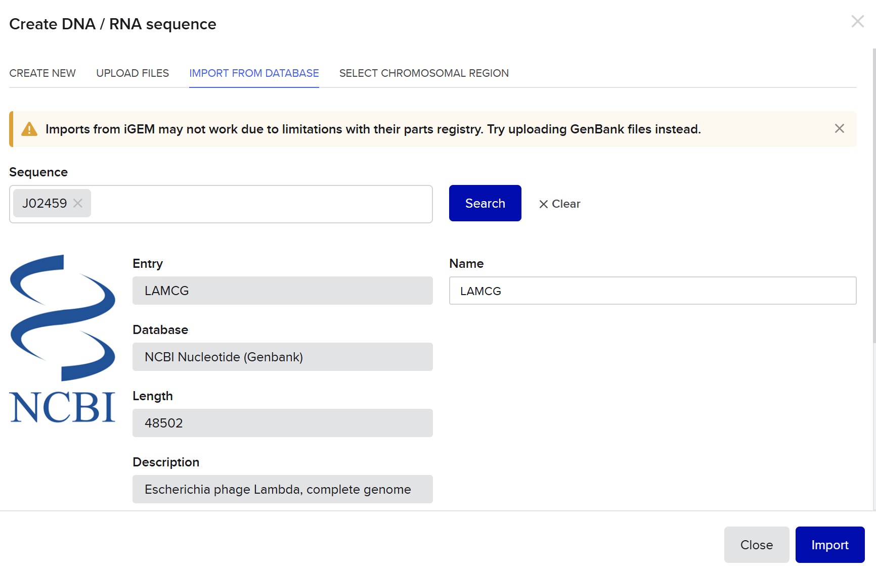
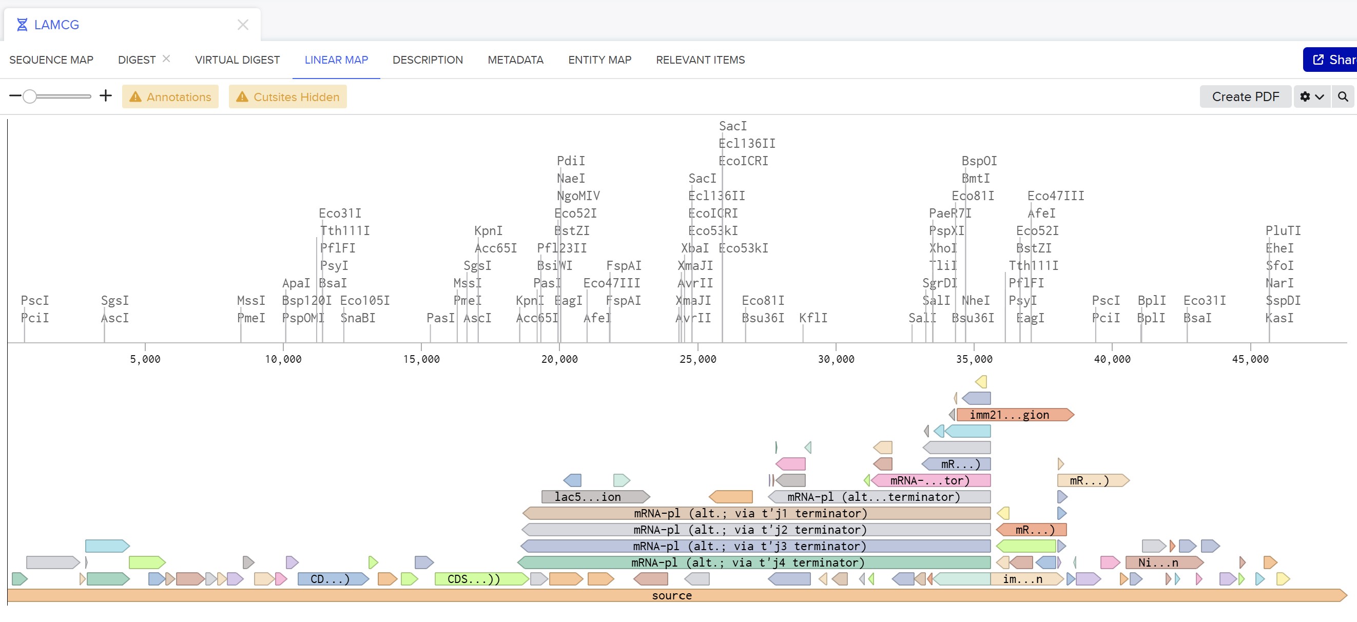
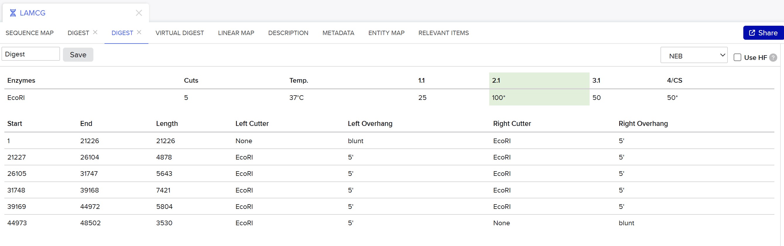
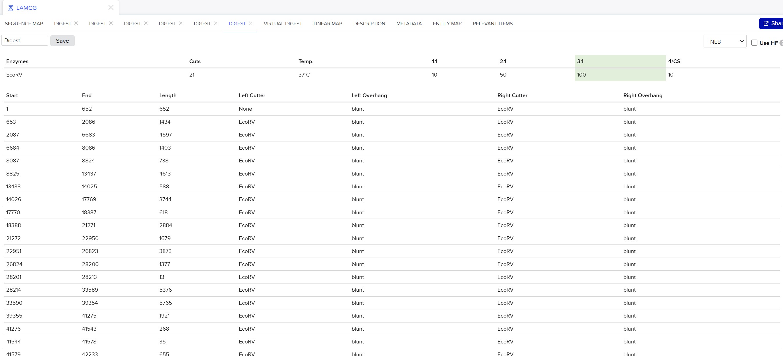
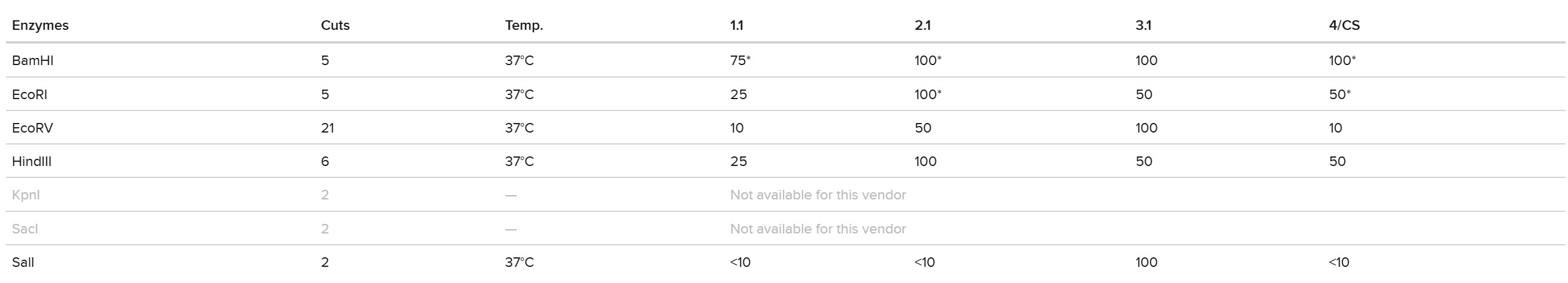
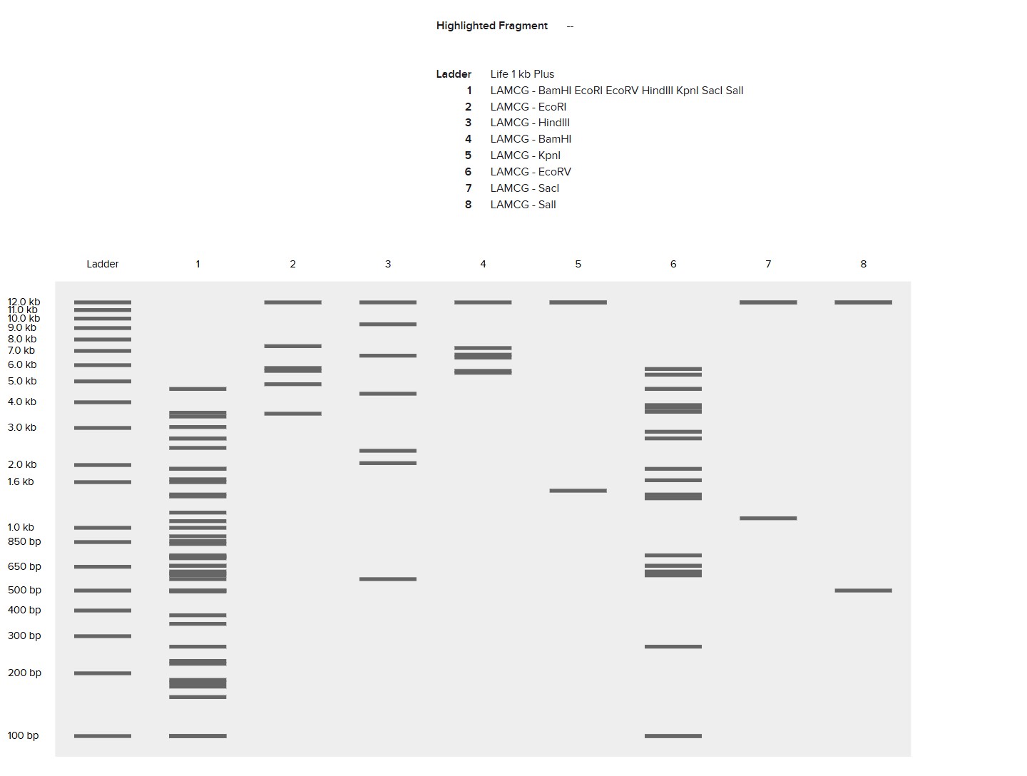
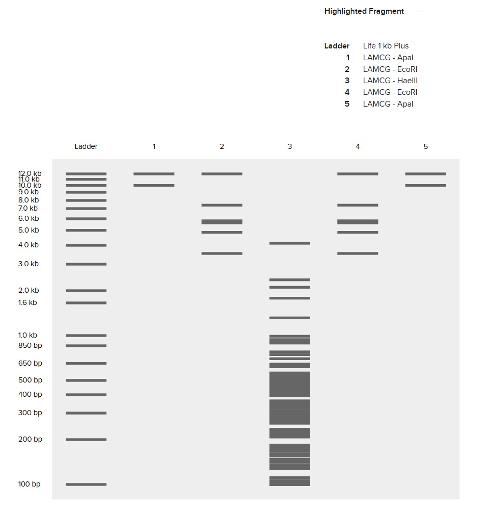
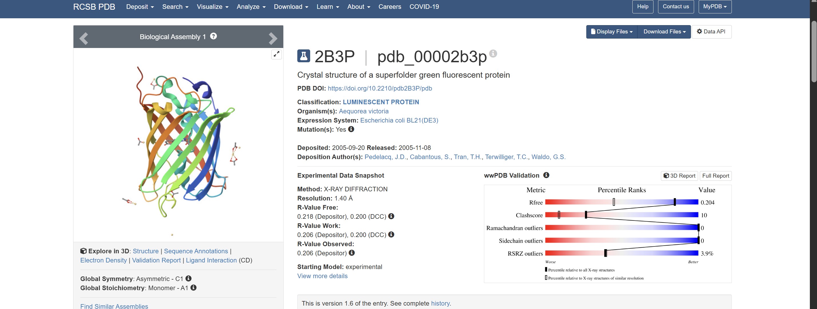
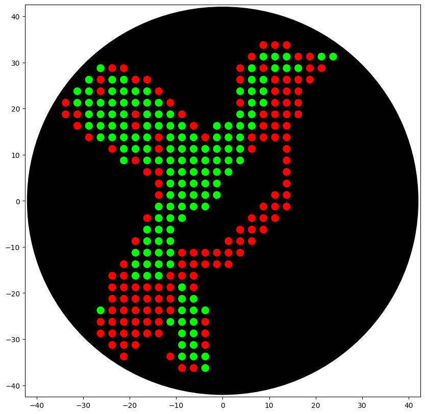
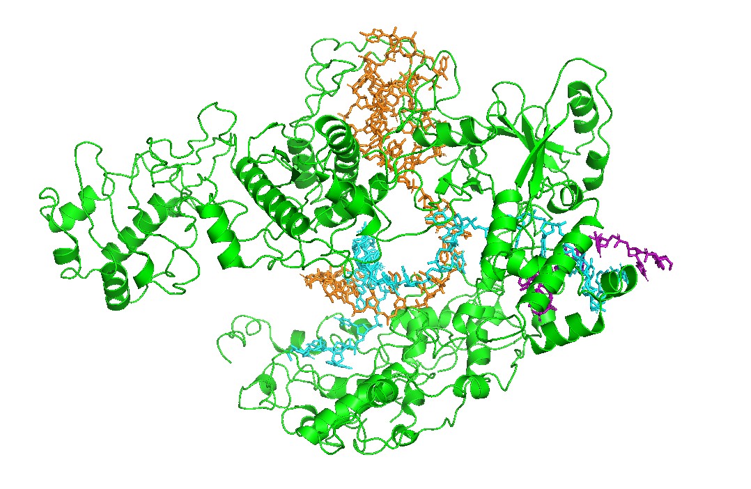

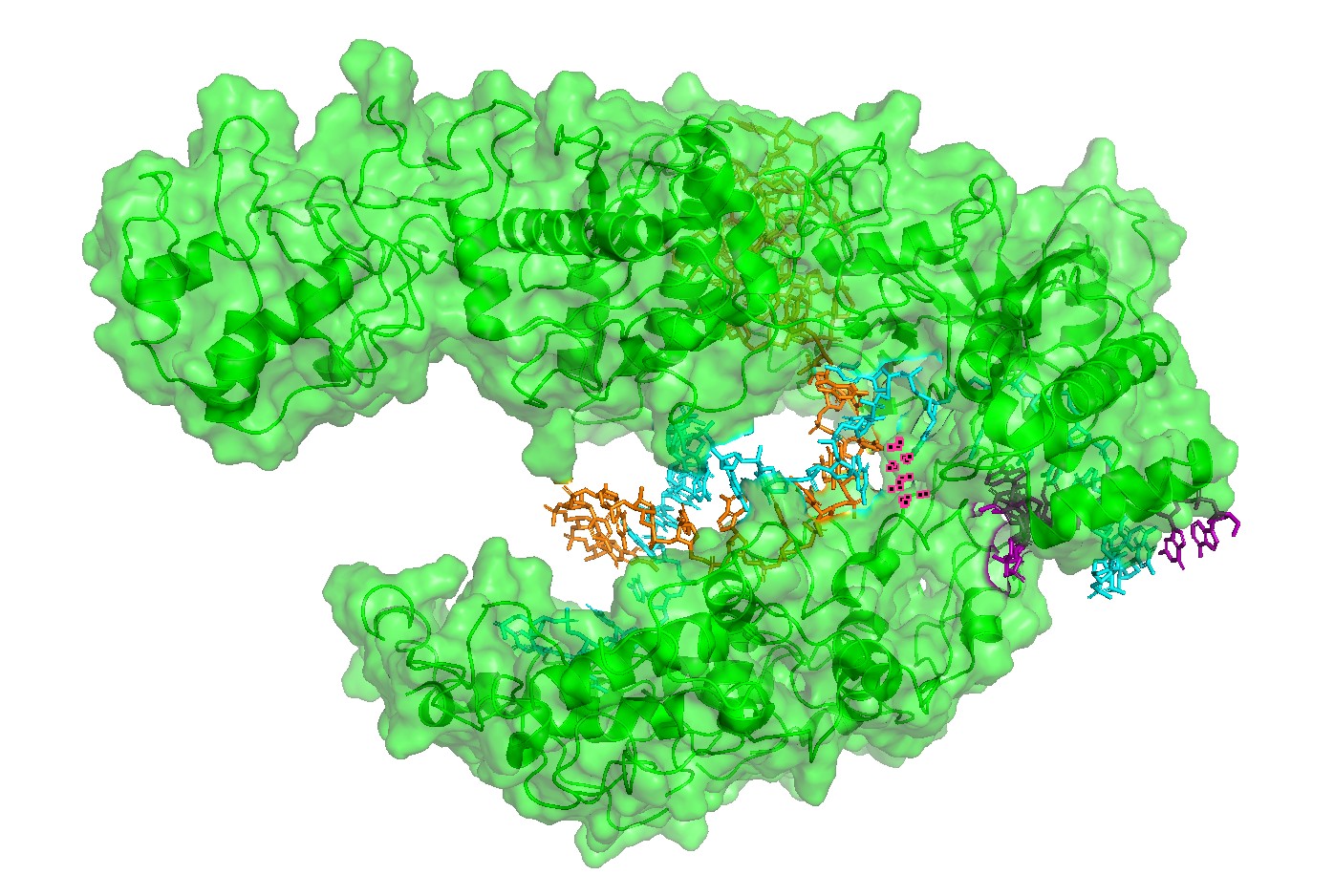
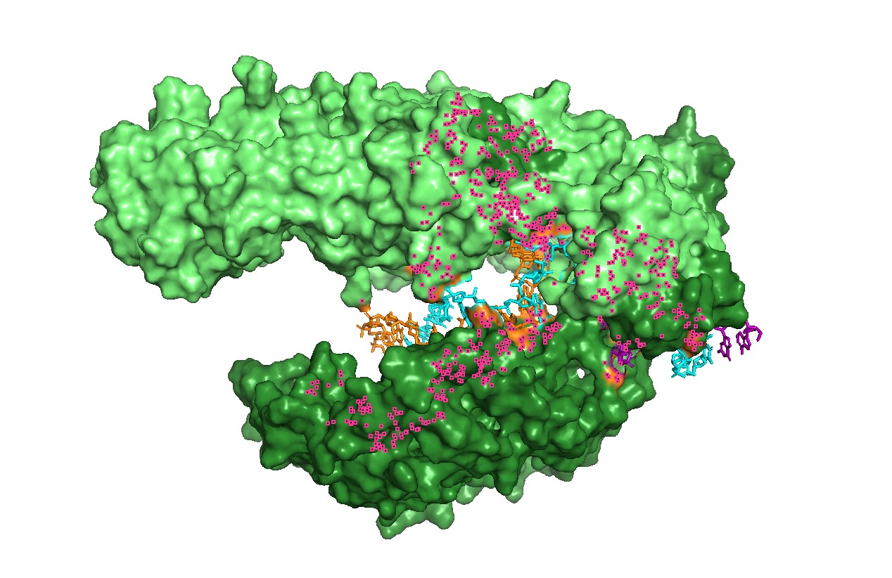
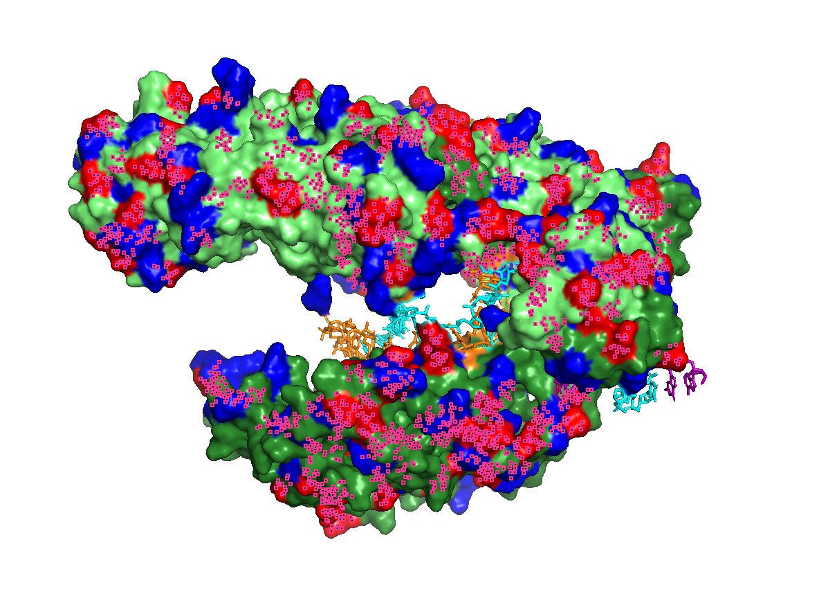
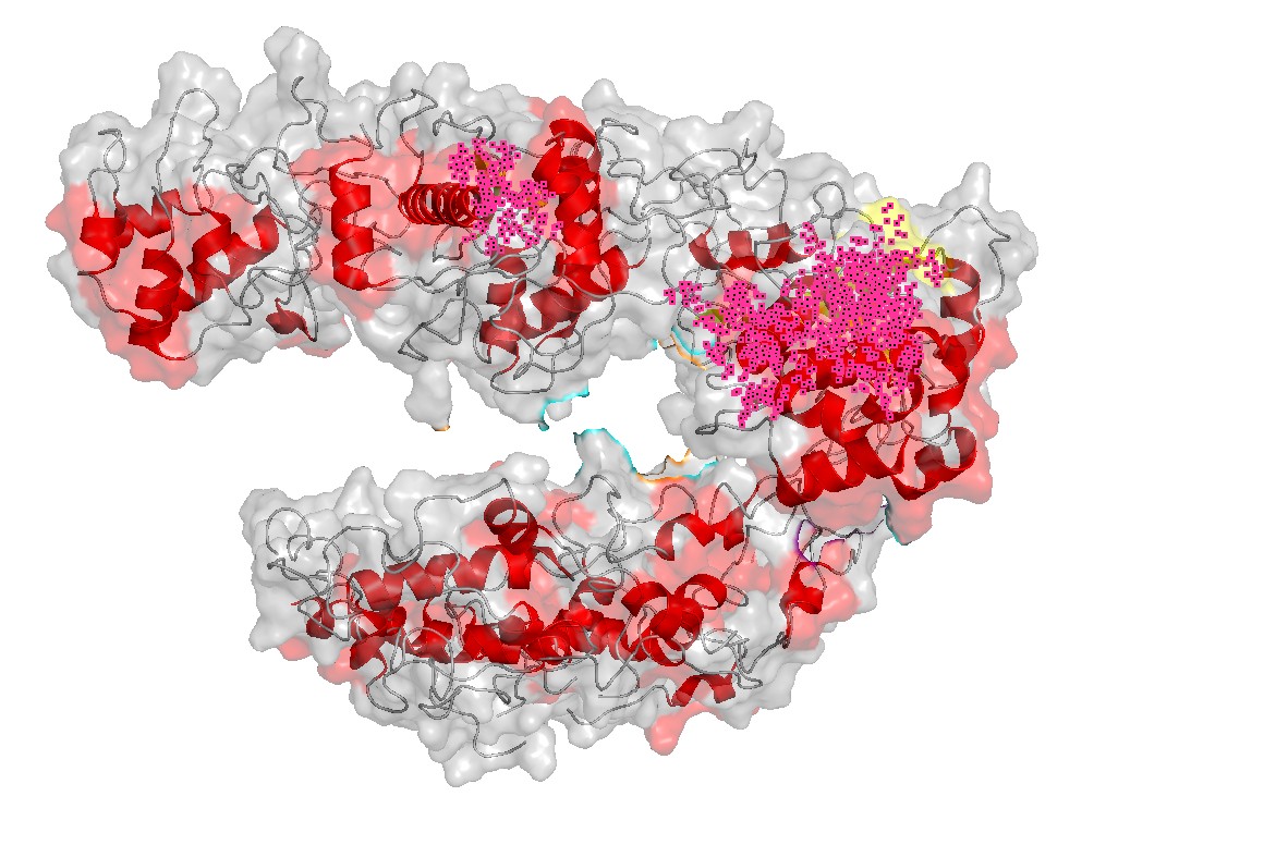
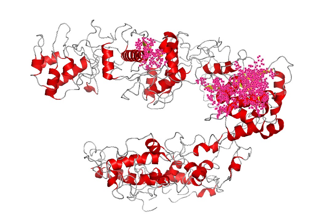
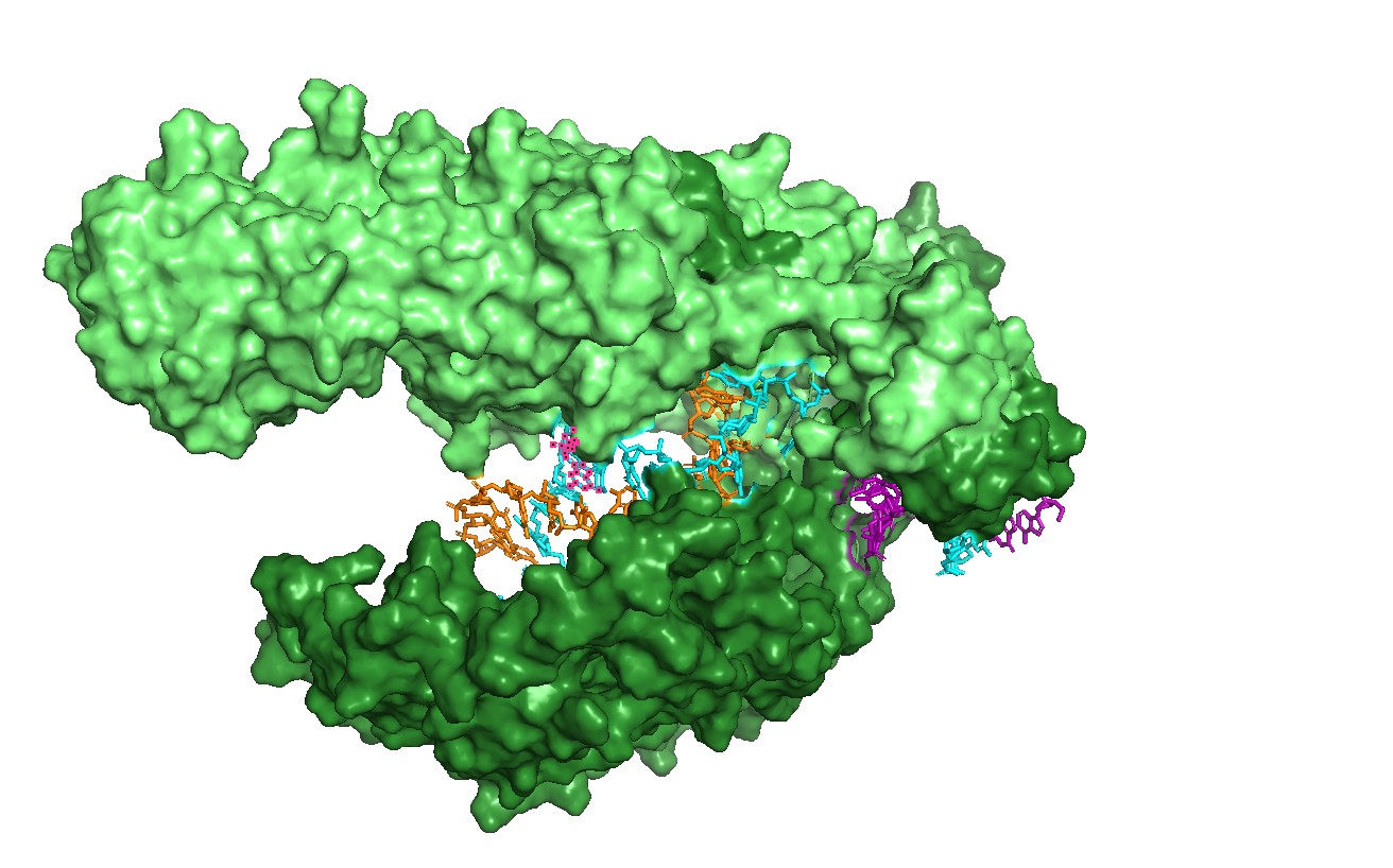
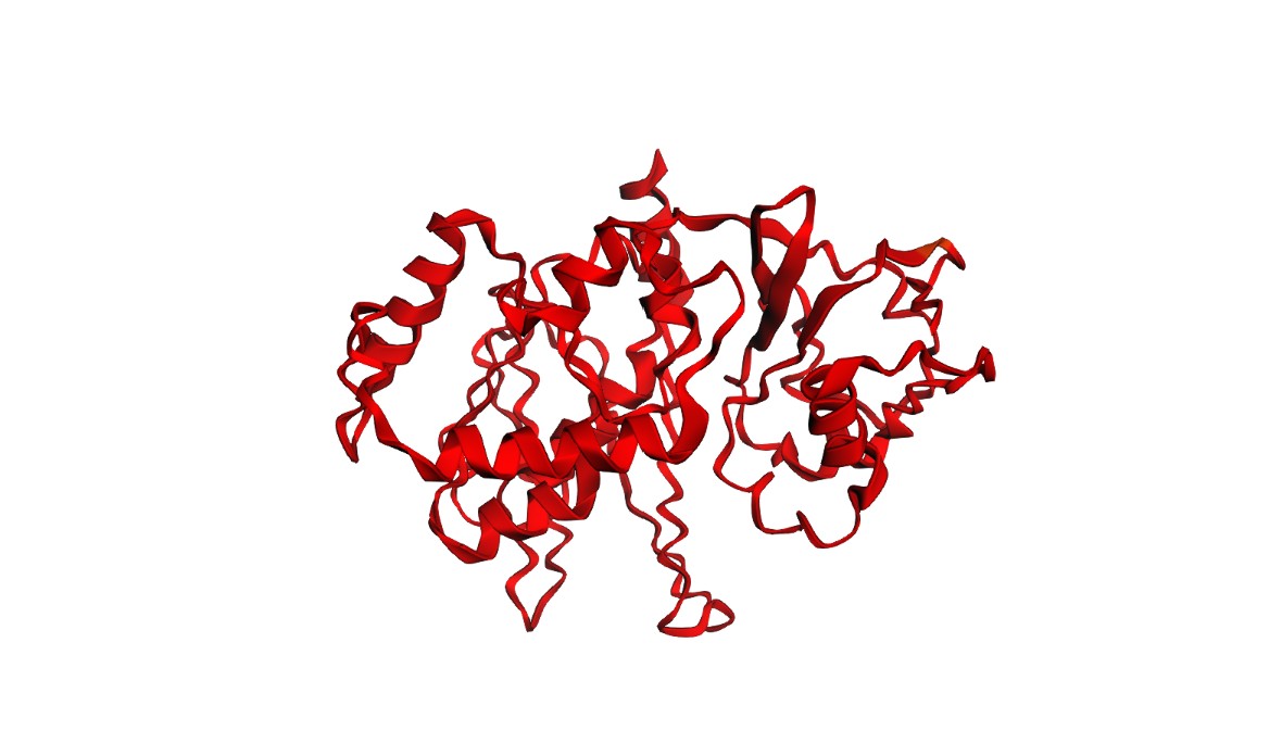
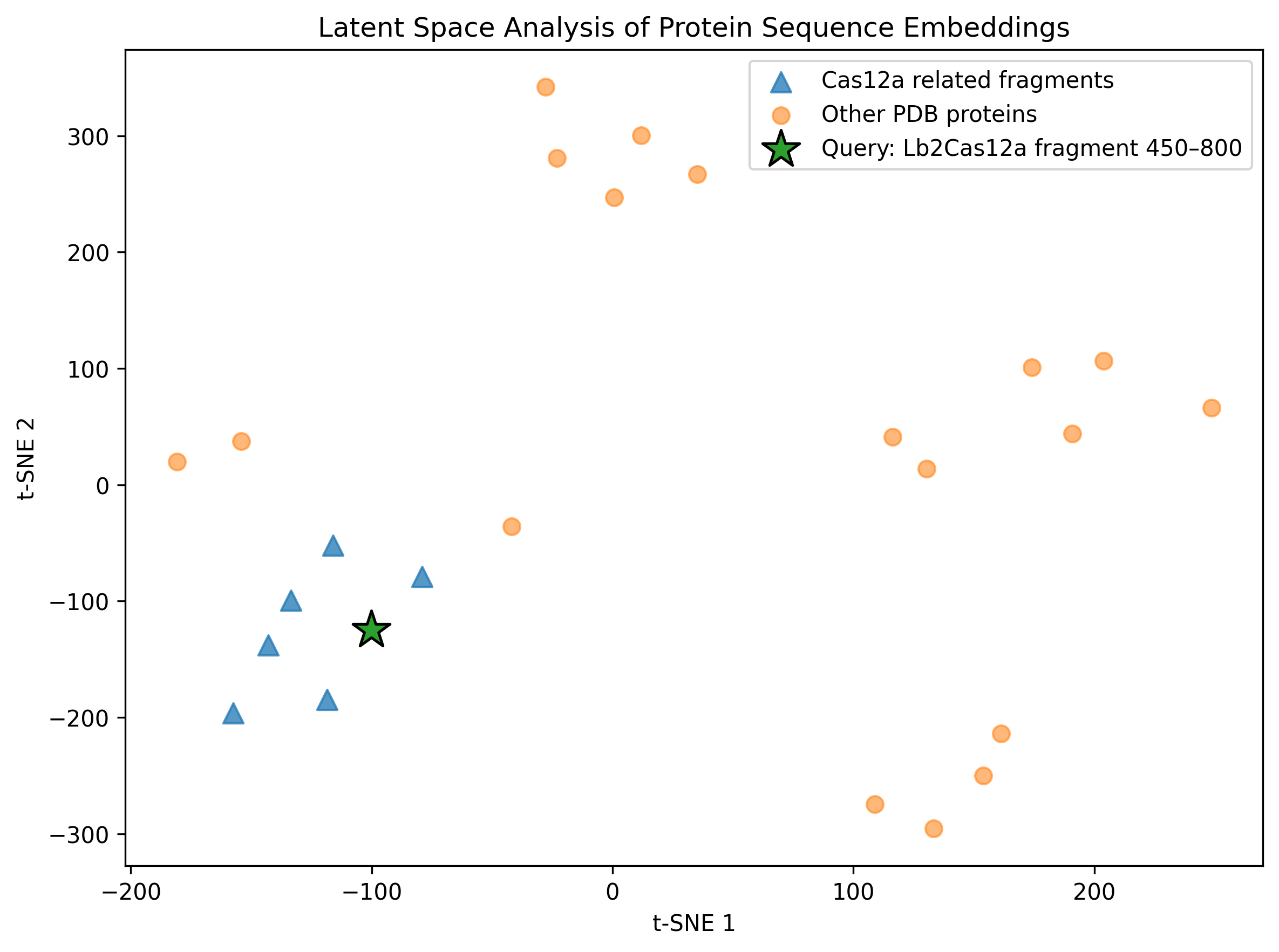
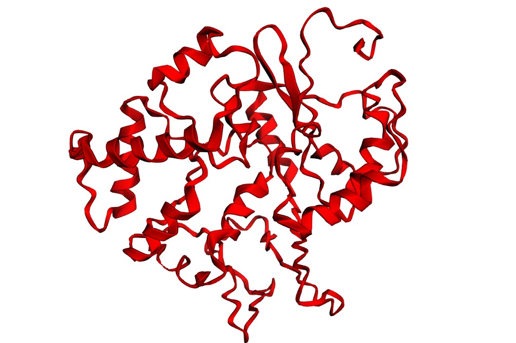
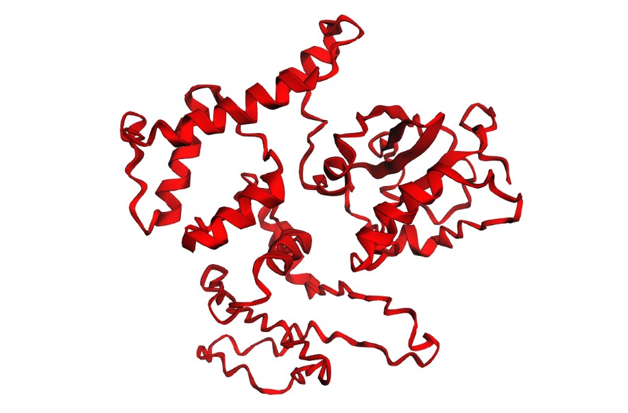
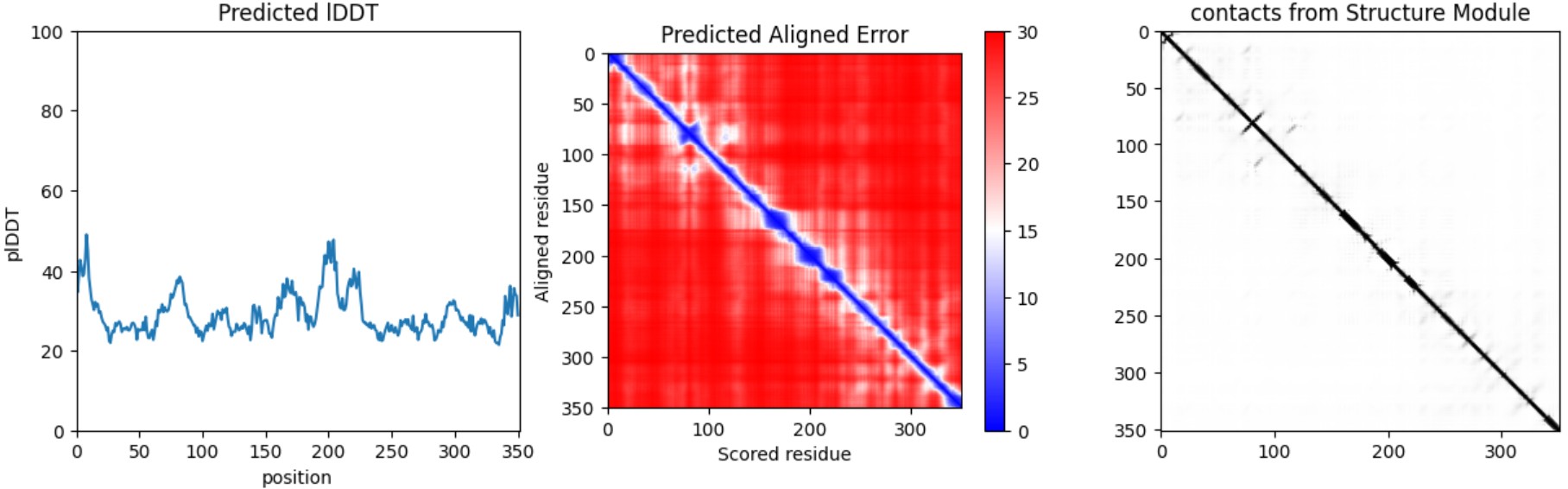
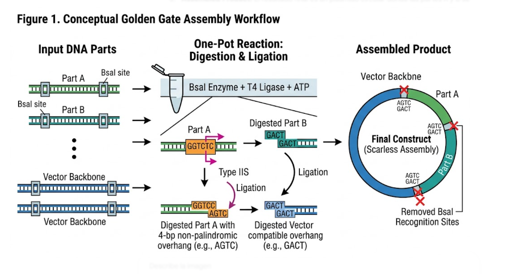
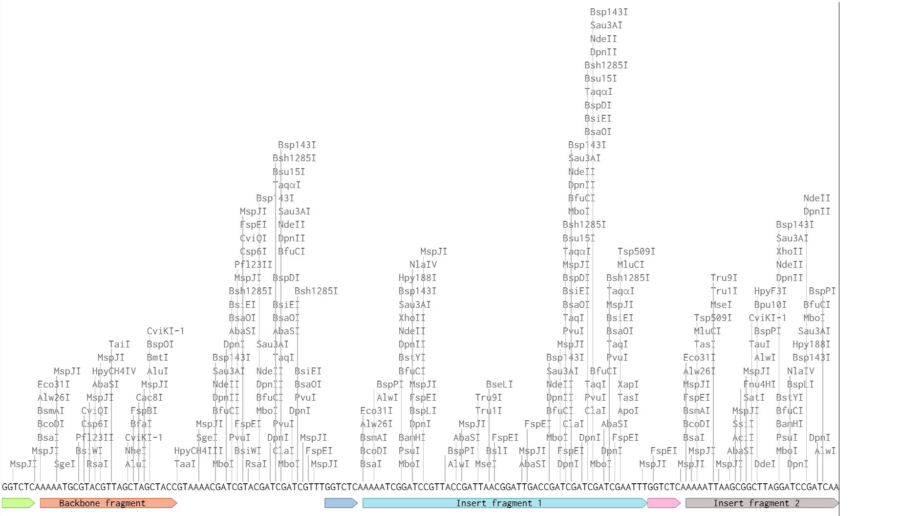
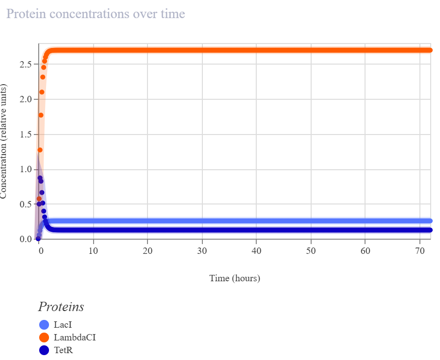
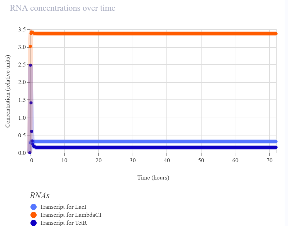
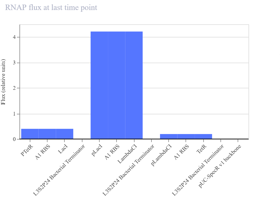
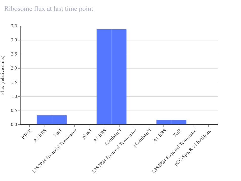
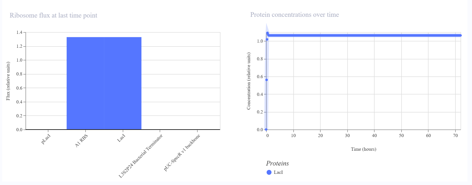
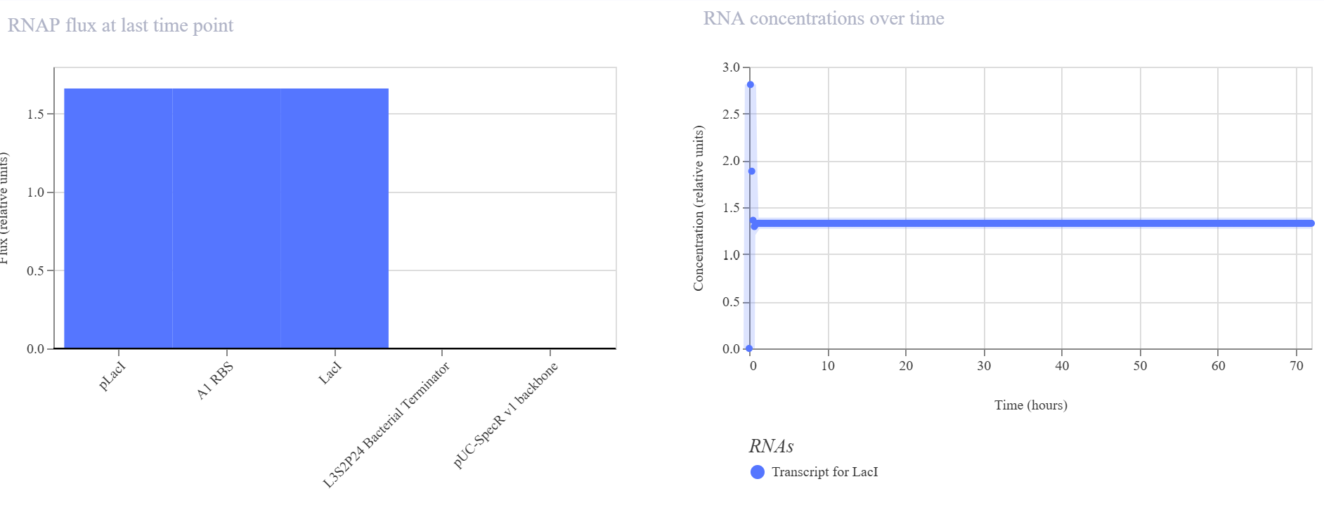
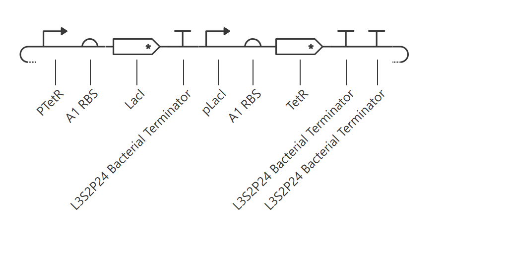

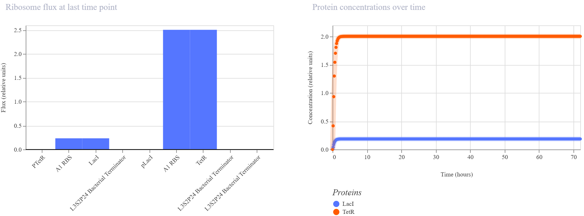
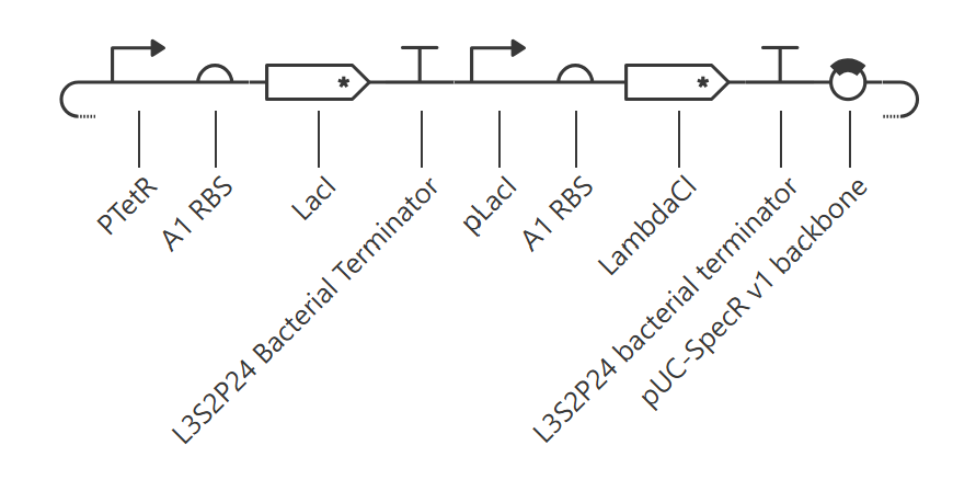
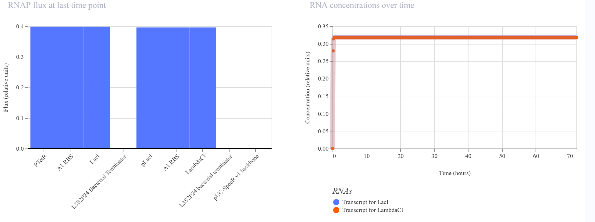
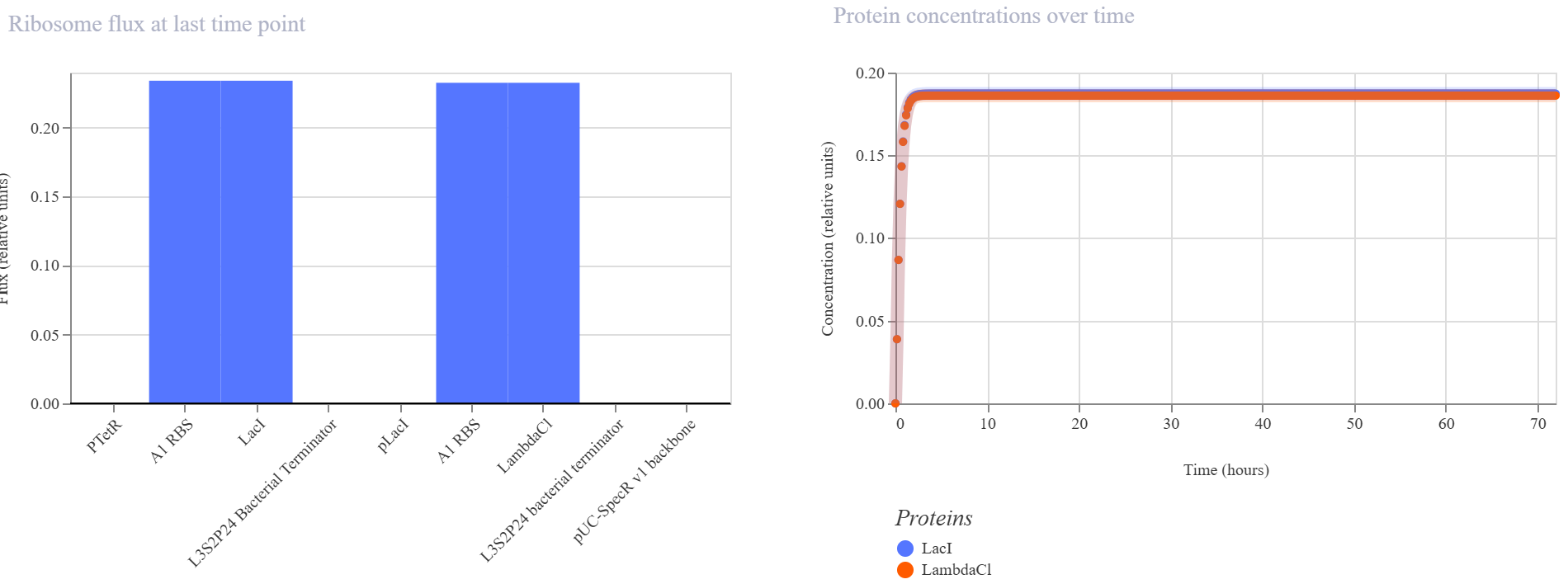
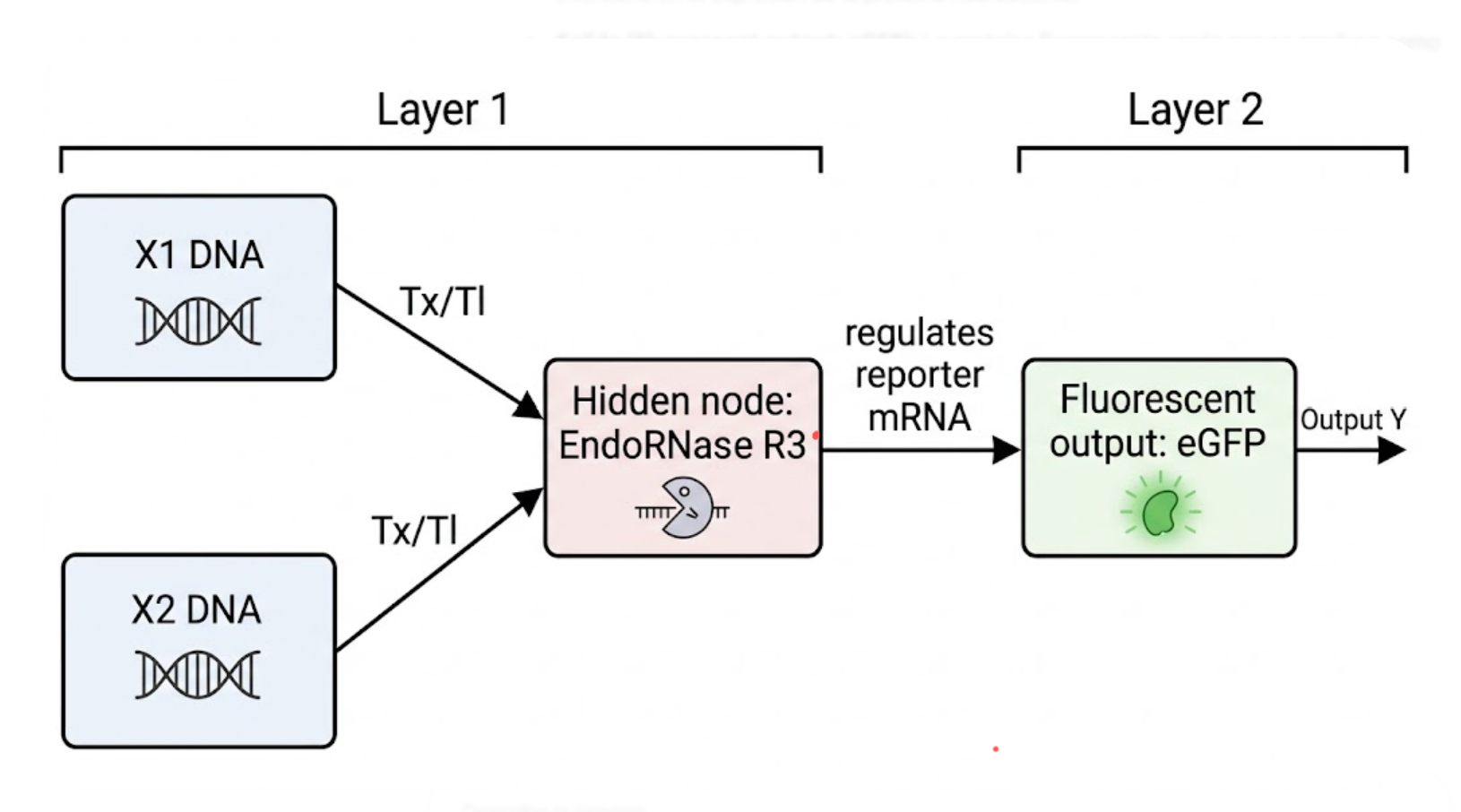
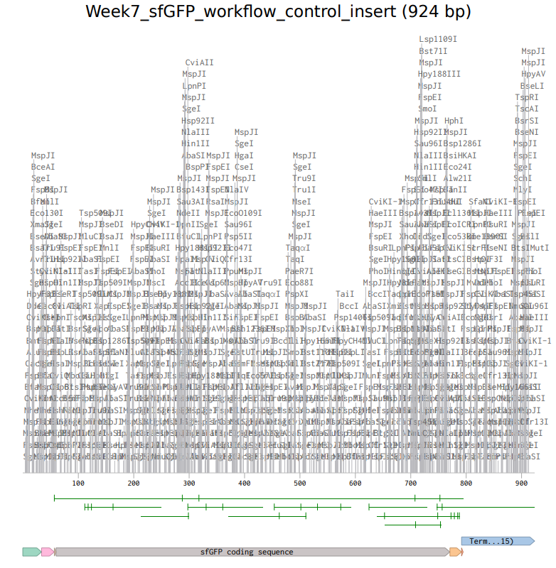
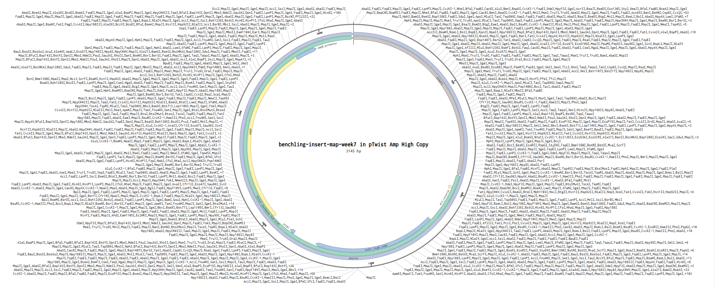
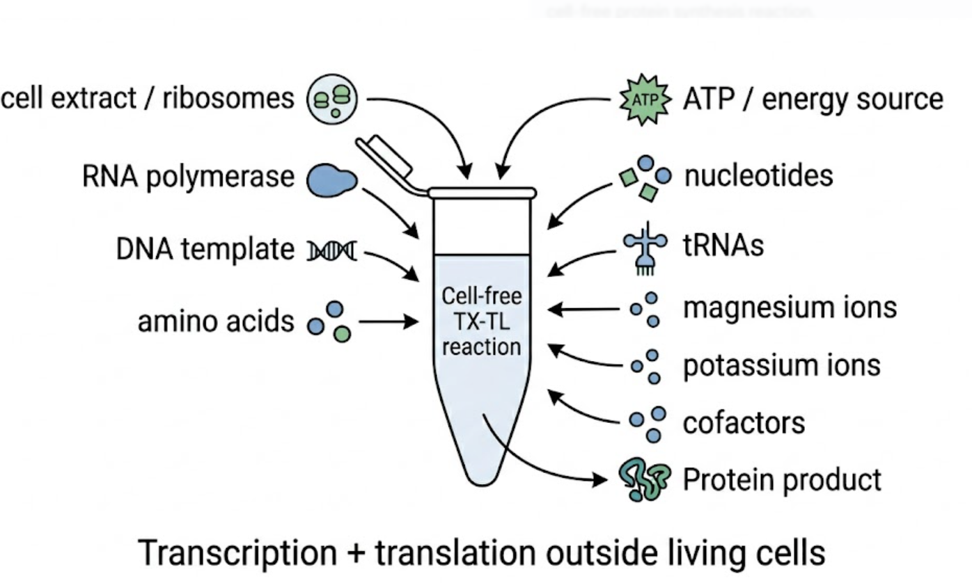
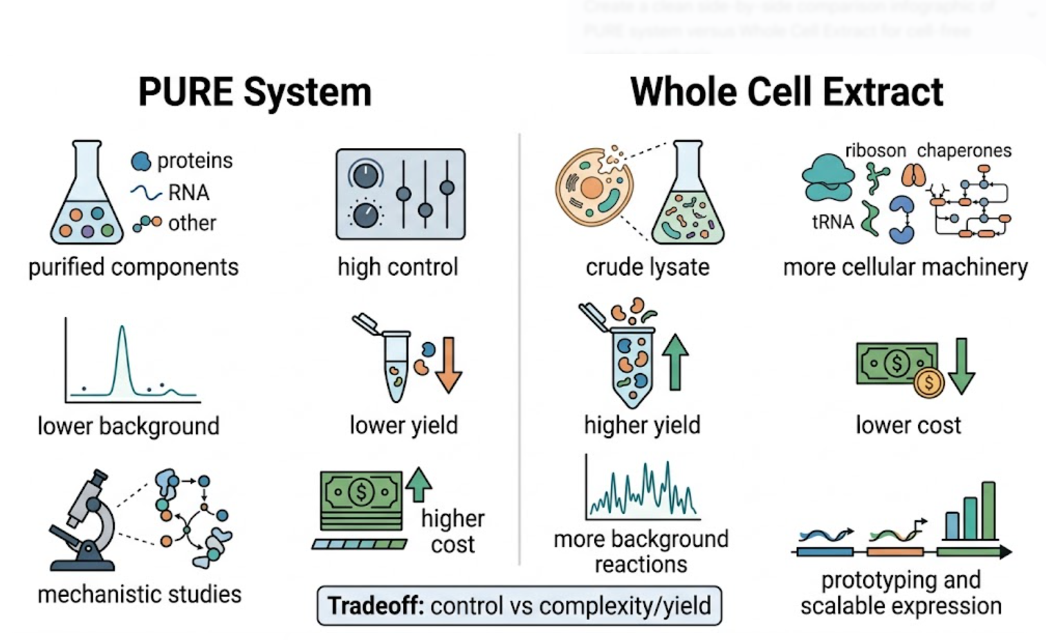
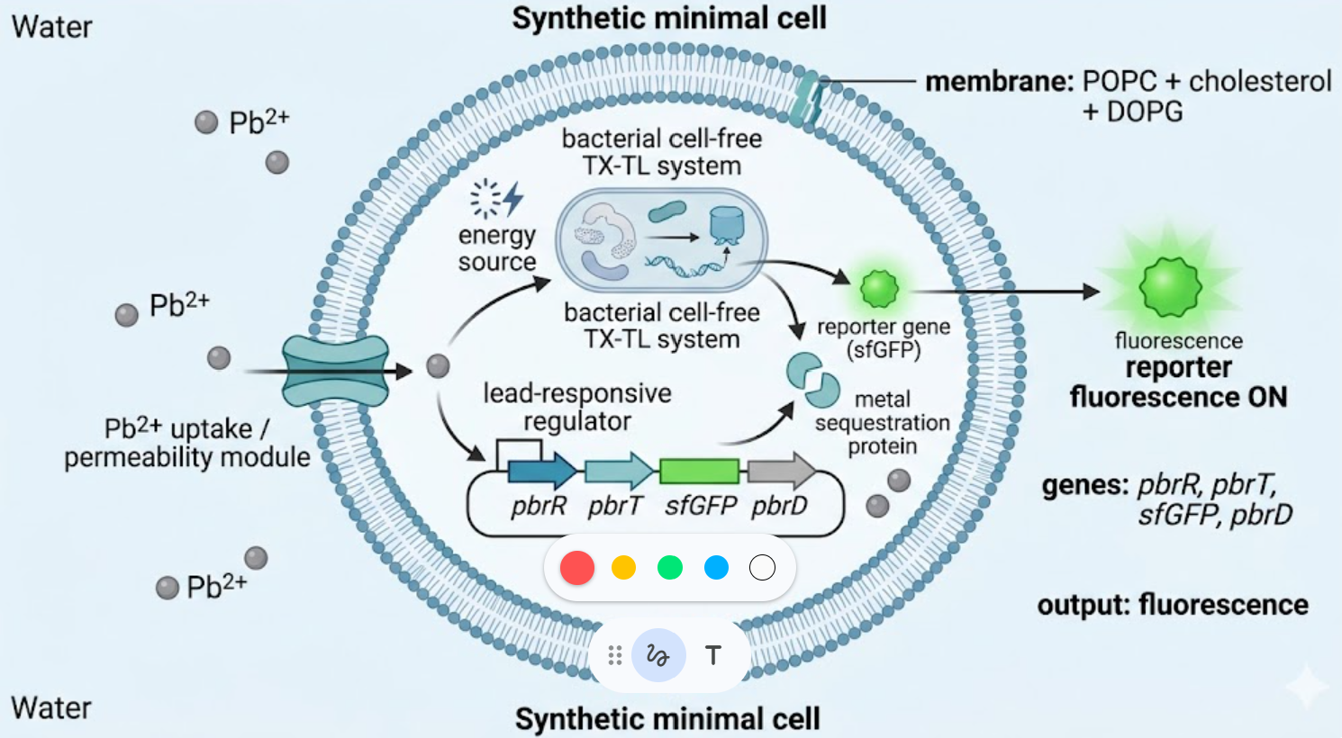
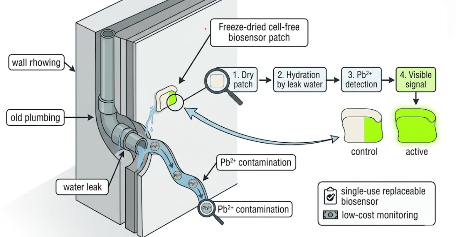
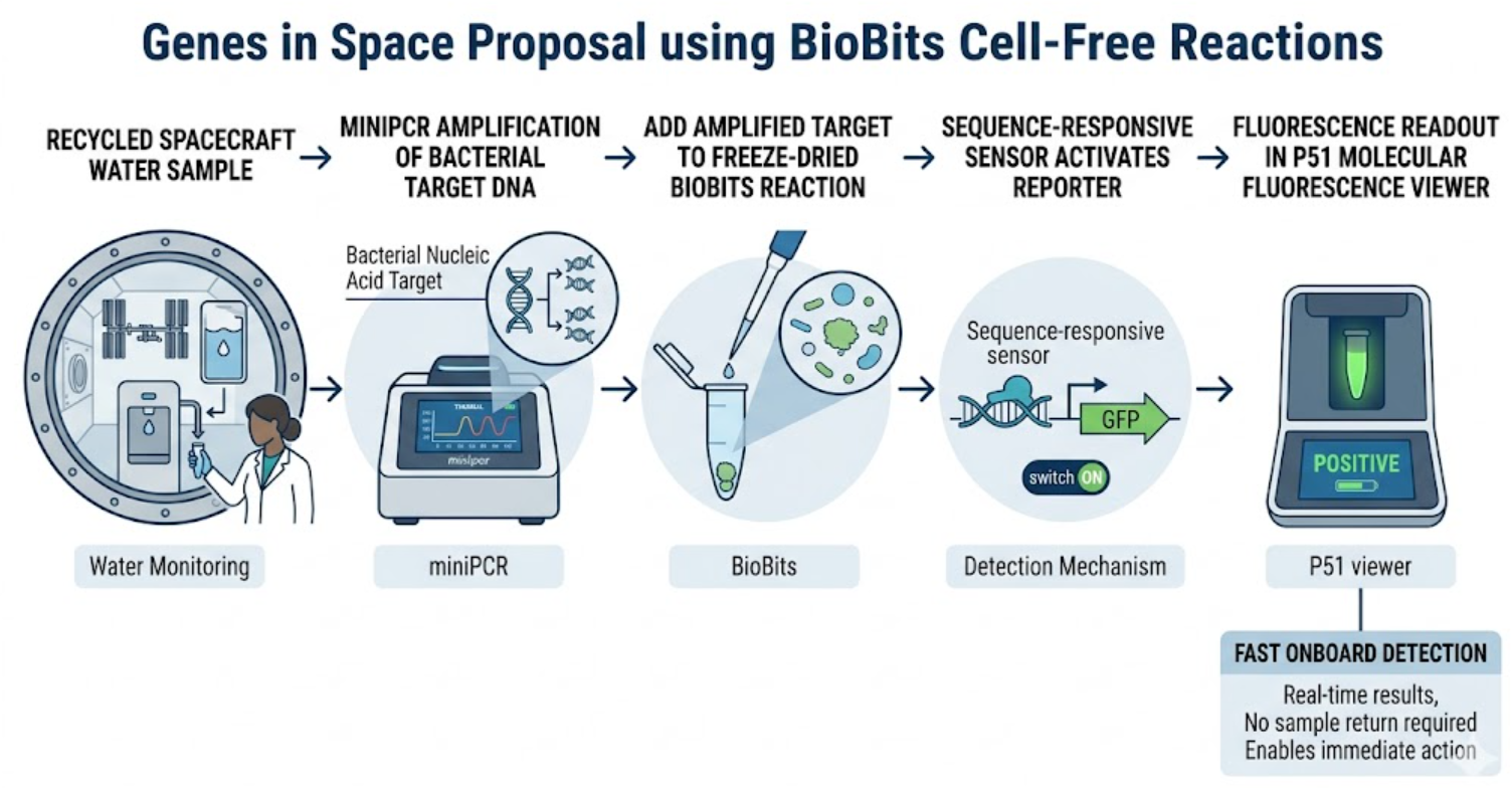

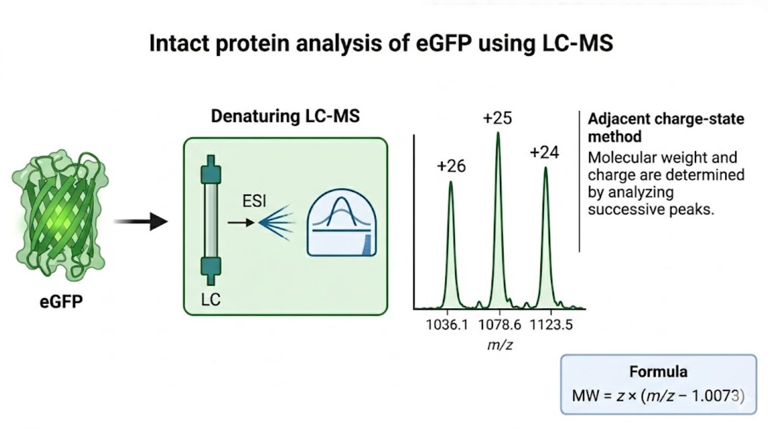
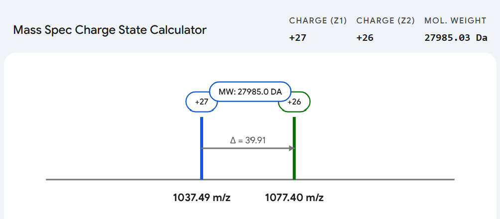
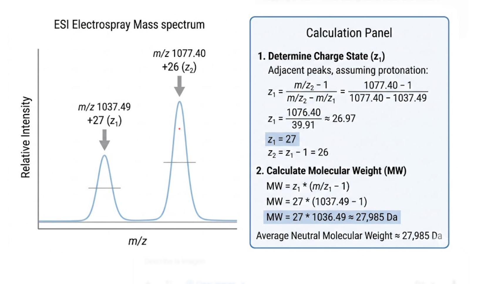
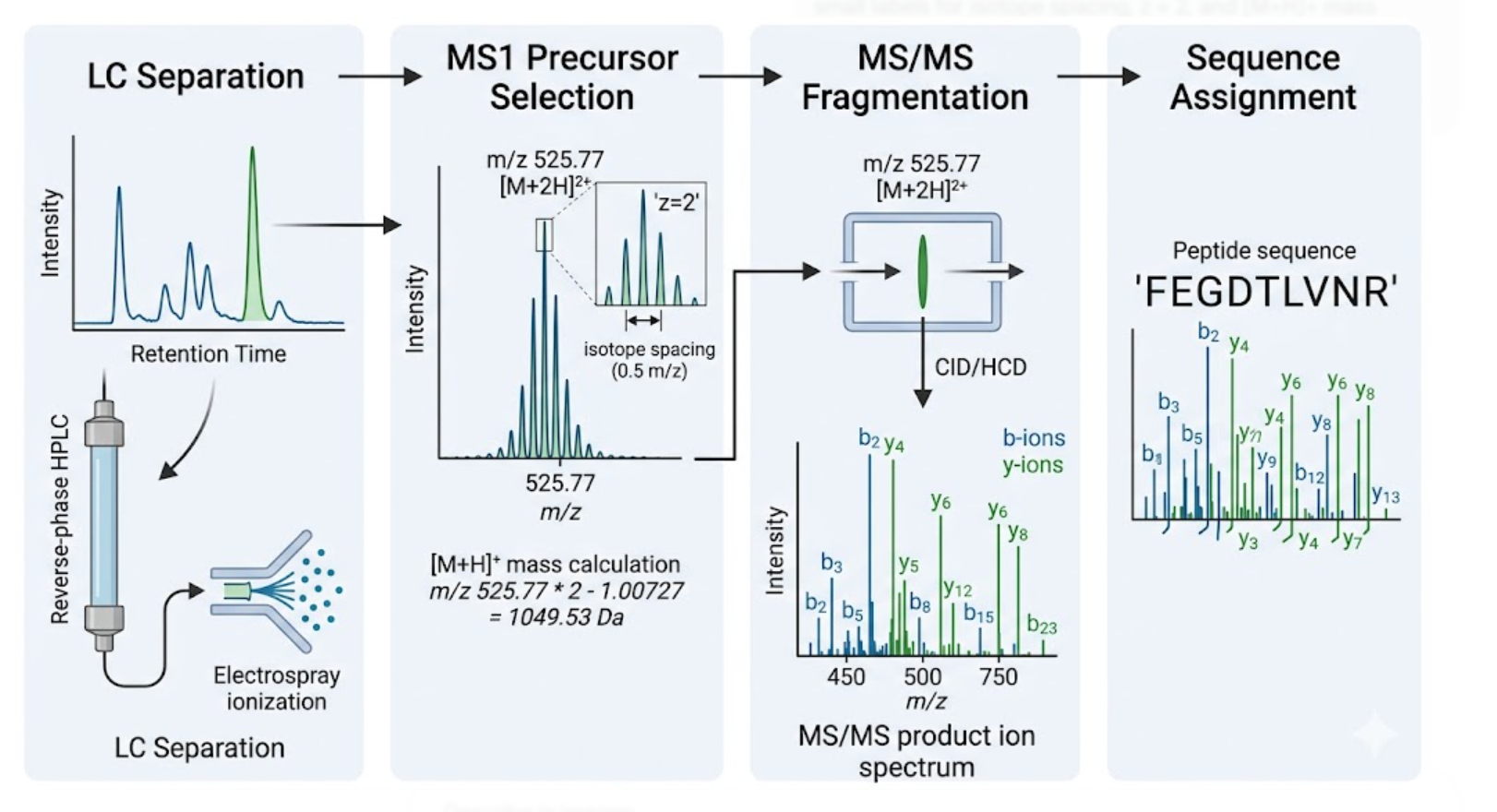
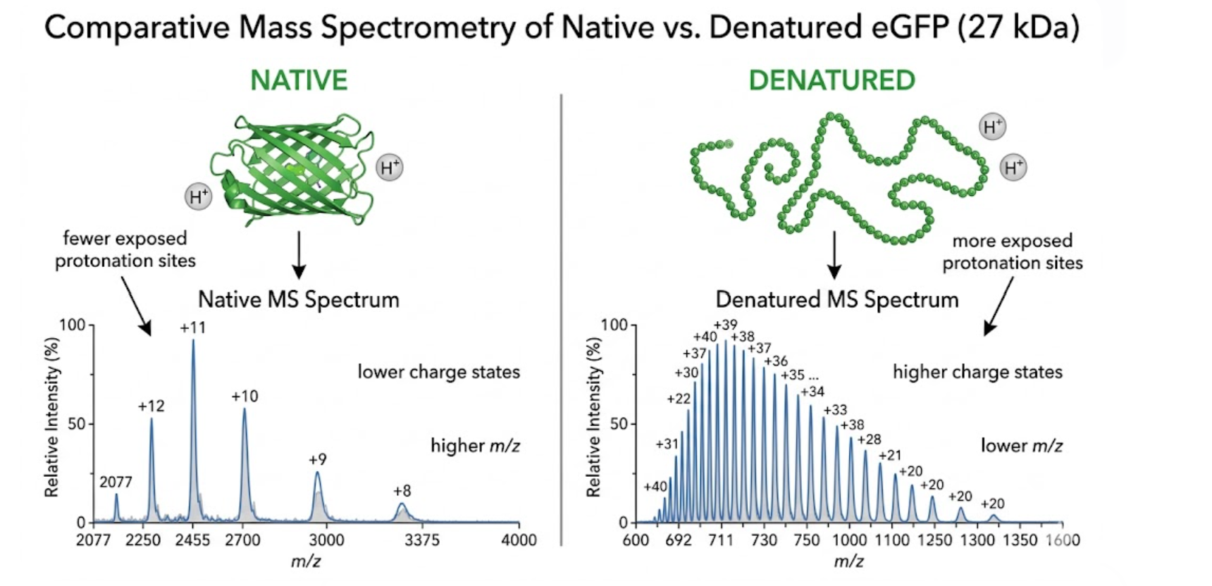
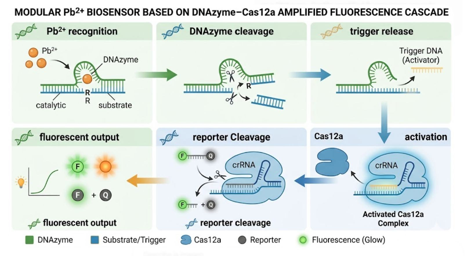

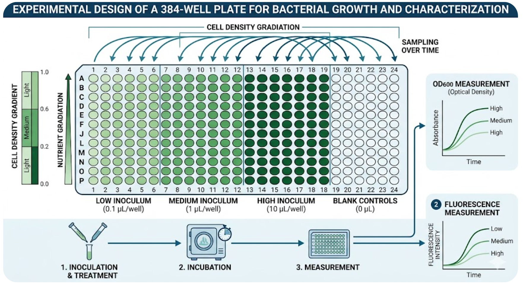
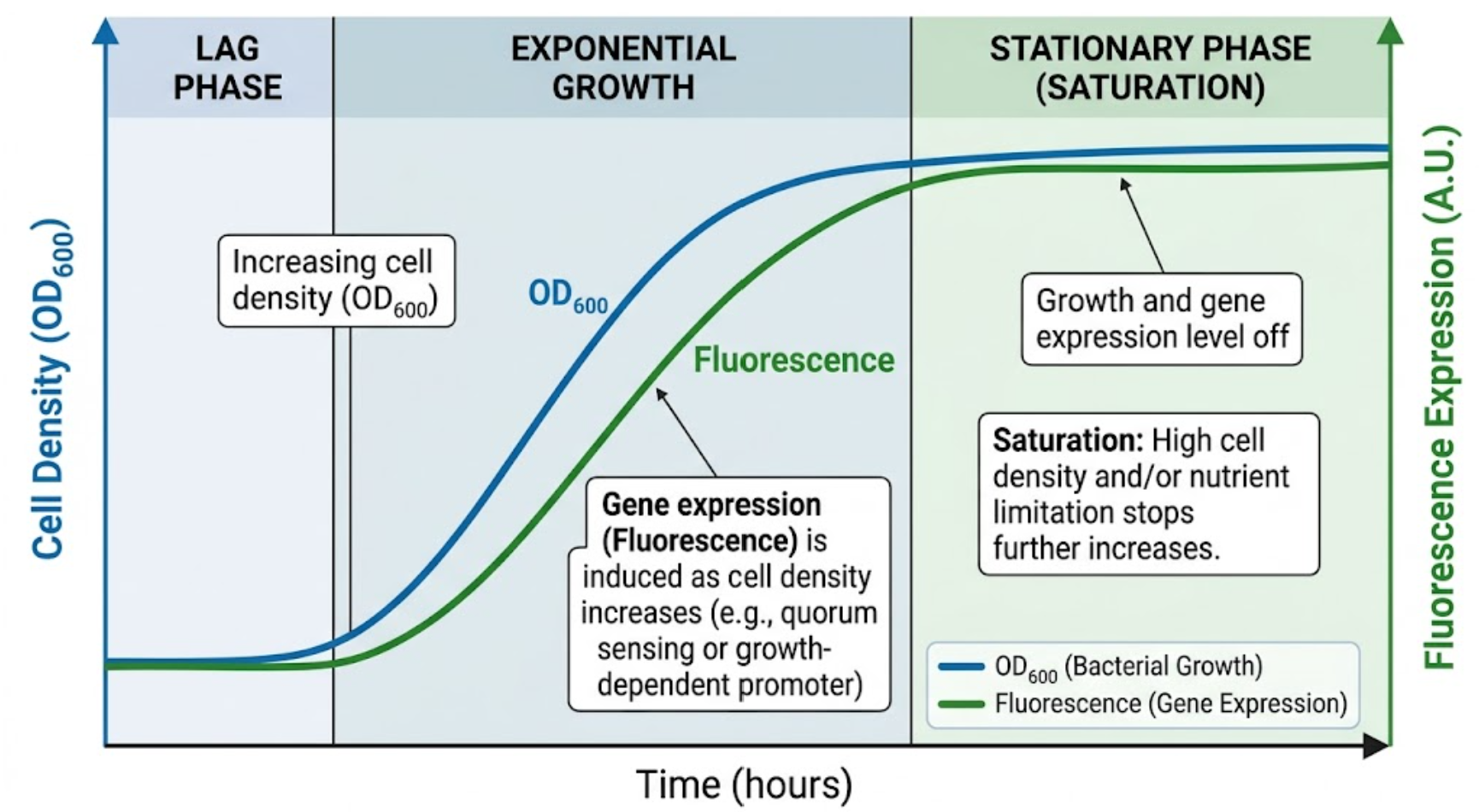
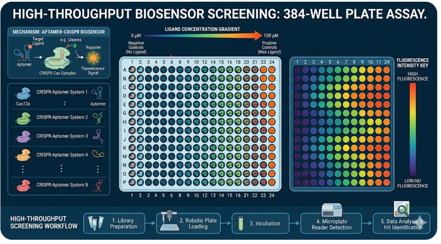
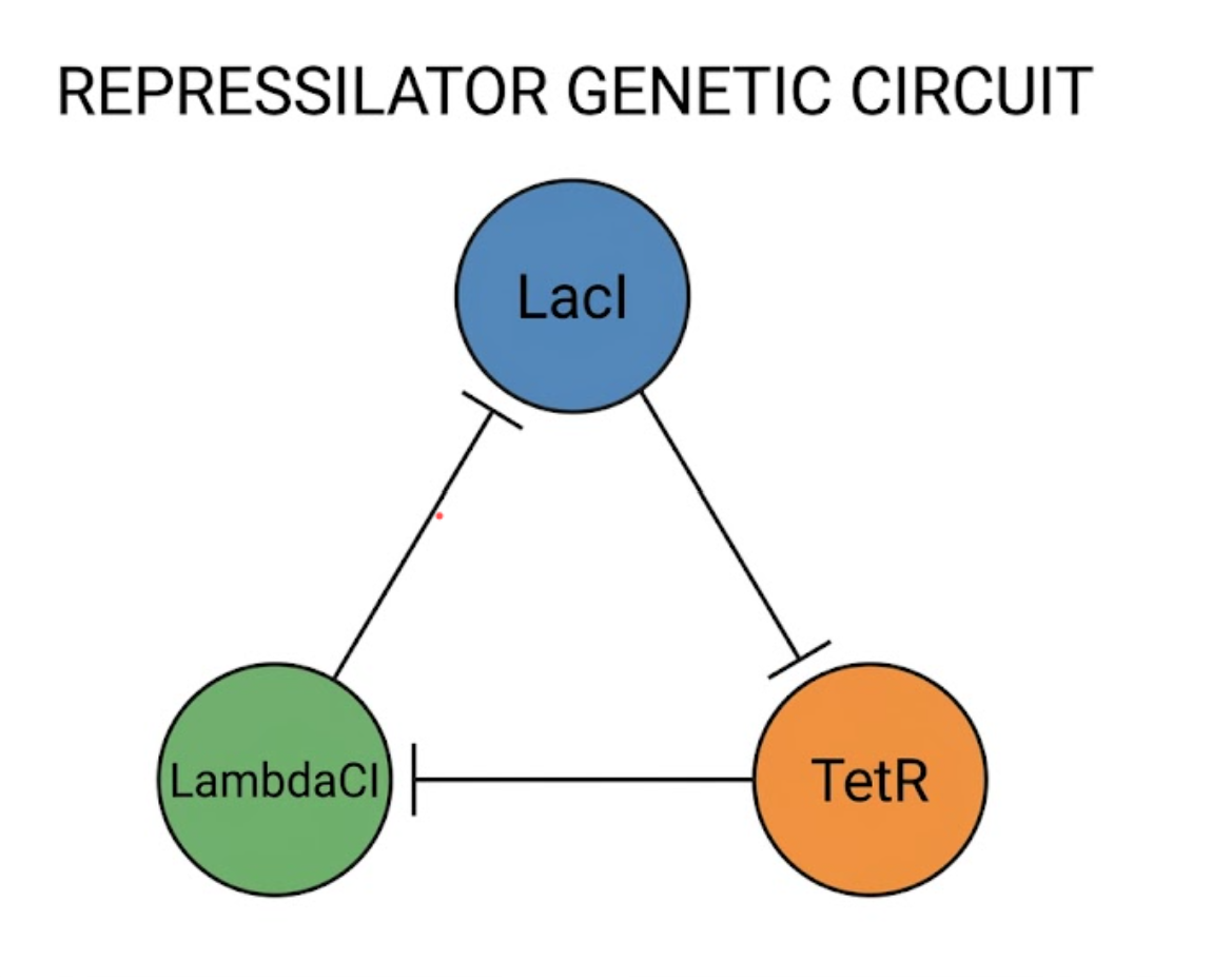

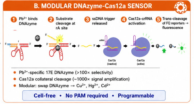
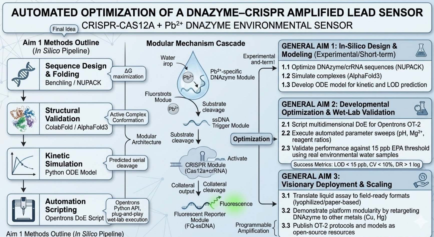
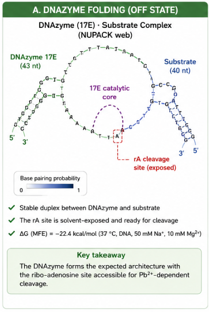
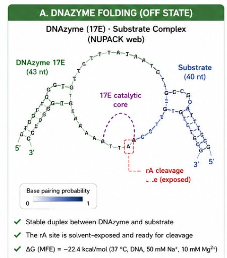

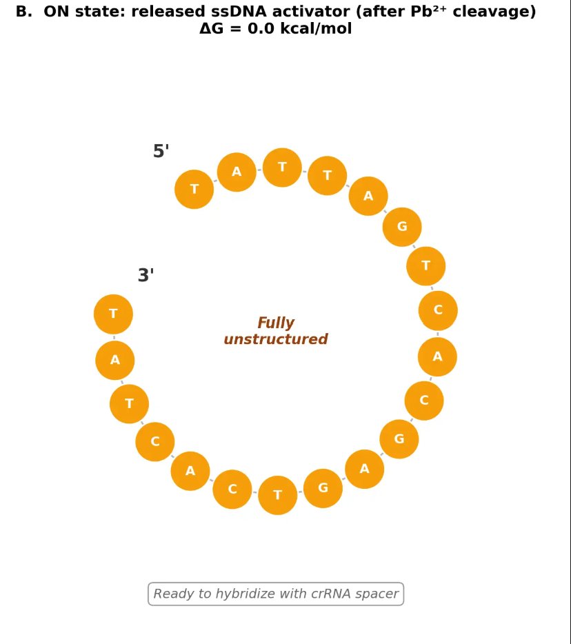
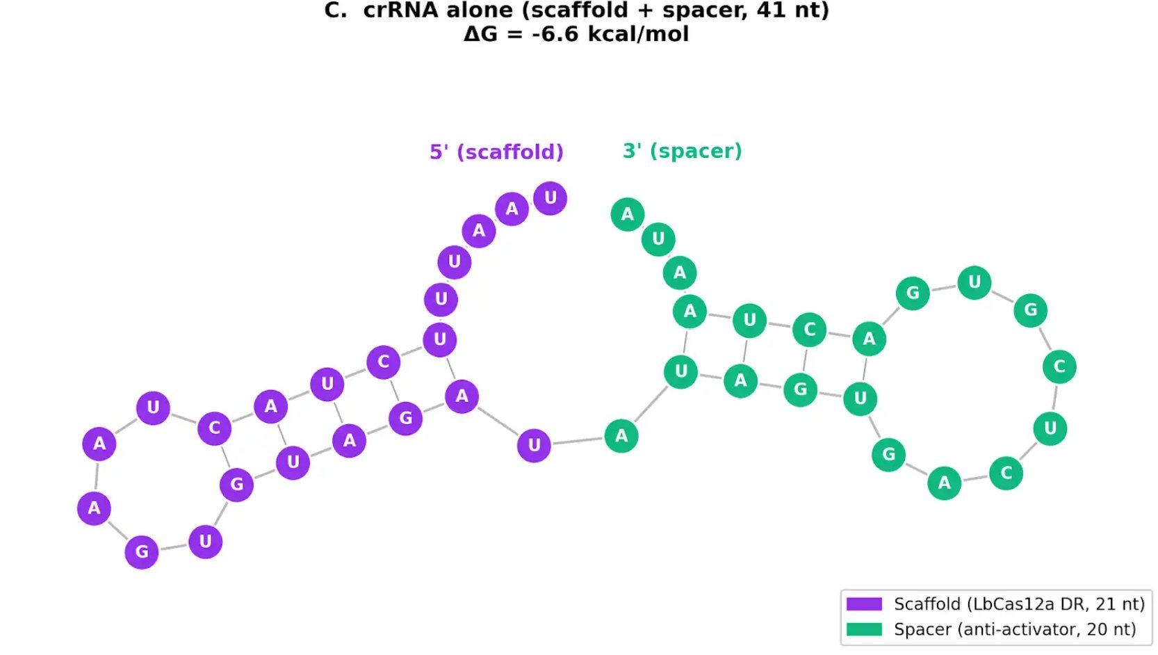
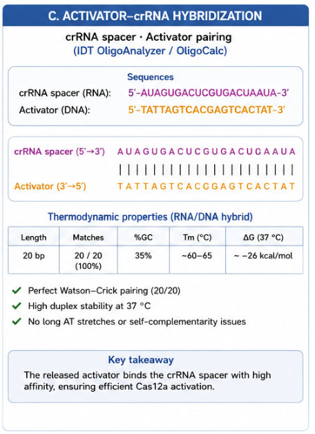
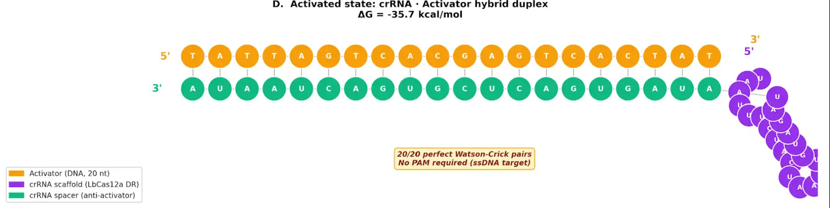
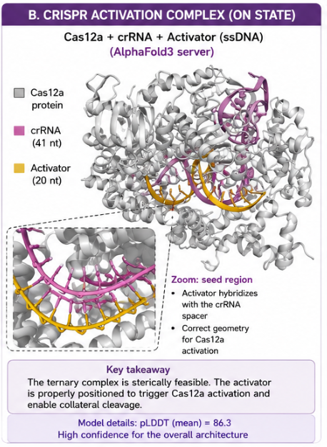
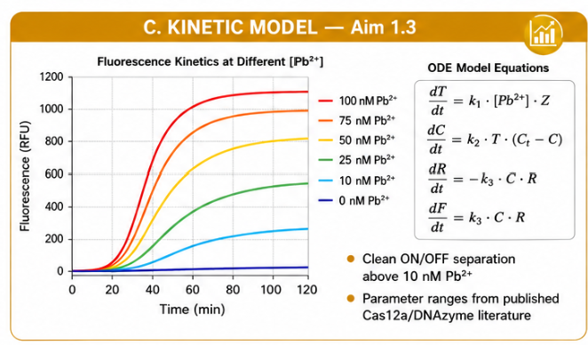
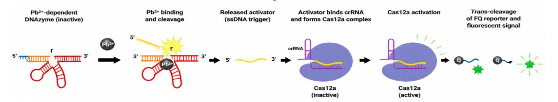
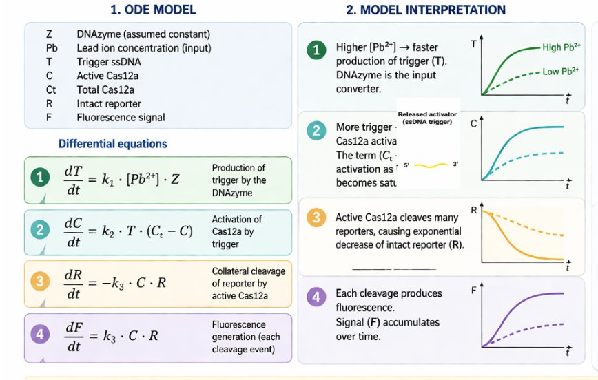
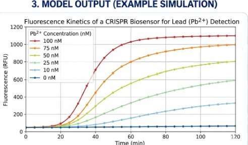
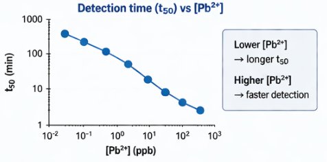
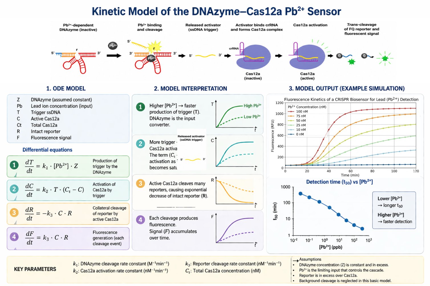
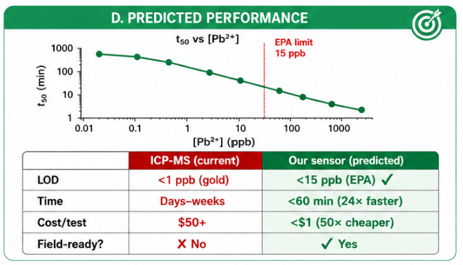
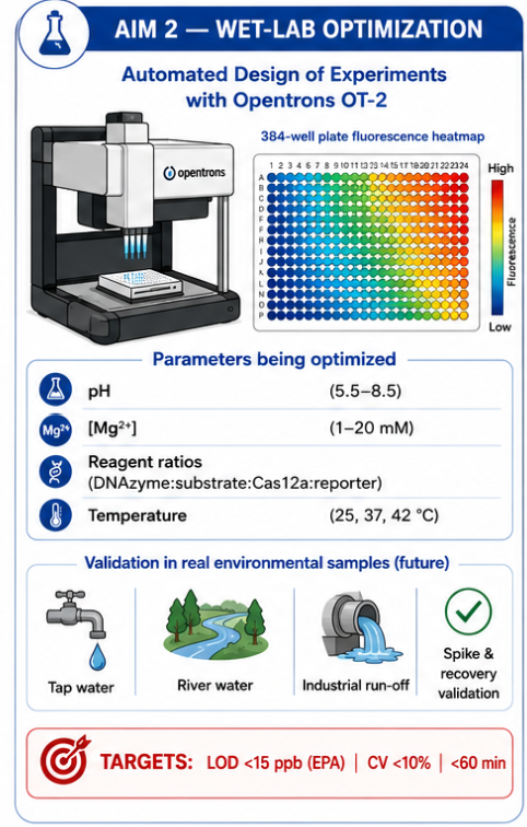
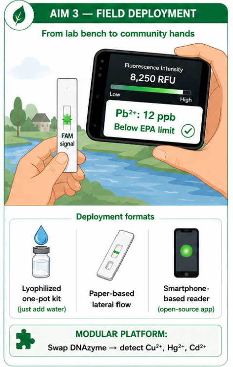
