Week 1 Lab: Pipetting

Week 2 Lab: Lab DNA Gel Art

Part 1: Benchling & In-silico Gel Art

Part 0a: Designing my Gel Art

For this week’s lab, I aimed to create a cool shape that would be easily noticeable and bring a smile to whoever sees it. After thinking through a few ideas, I decided to try creating a rubber duck shape :)

To start designing, I took a picture of the gel alongside the ladder from Ronan’s website and copied it into Procreate on my iPad. Then I added guiding lines in the common areas where many of the segments from the randomizing tool appeared, and sketched the overall shape of a rubber duck.

Very quickly, it became clear that a rubber duck isn’t an “easy” shape to create with this technique. Because it is full of curves and the resolution is relatively low, getting a clear shape was much harder than expected.

To make it more visible, I tried enlarging it to cover more potential segments (i.e., the image’s pixels), but it didn’t work the way I intended. After thinking it through a bit more, I decided to create a HEART! This too is a very curvy shape, but it’s definitely simpler than a duck - and it’s also Valentine’s Day in two days!

So I did the same thing and got the following basic design:

Once I was happy with my design (and honestly, while designing it), I started thinking about how I could determine which enzymes to use to make all of the DNA segments in the specific sizes I wanted. I realized the best and most efficient way for me to go about it was to use Ronan’s website again. I used the “randomize” tool again, only this time I did it for only one column at a time, to get familiar with all of the different combinations of 2-enzyme cuts I could get. It turns out that this number wasn’t very big (55 to be accurate — 45 from pairs + 10 single enzymes), and the options were limited. Since I didn’t want to use 3 or more enzymes, I had to work with this.

To be able to design through the website, I first got myself familiar with the different possible combinations of digestions, and then tried to search for the closest match to my original sketch. After a few tweaks, I created a design I was satisfied with and was ready to move on to the next step!

Part 0b: Expected Results and Walkthrough

I then moved on to Benchling to transfer my design there by uploading the Lambda DNA and adding the corresponding restriction enzymes. After a few digestions, I noticed something weird — the HindIII enzyme cutting sites on Ronan’s website didn’t match the ones on Benchling. This means that my heart design didn’t look like a heart anymore :(

So I went back to Ronan’s website and tried to find alternatives with the hope that I would find them — and I did. The new design didn’t look as rounded as I wanted, but it was certainly a heart, and I went with it! Here is the Benchling design:

And the equivalent design in Ronan’s website:

And so I moved on to the next step!

Part 2: Gel Art - Restriction Digests and Gel Electrophoresis

Part 1a: Preparing a 1% agarose electrophoresis gel

I created the gel solution and poured it into the gel tray. Weighing the agarose and measuring the TAE buffer:

Pouring the solution into the gel tray:

Then I let it set and moved on to the next step!

Part 1b: Restriction Digest

Here I again followed the protocol for digesting the Lambda DNA with my chosen enzymes: Pipetting:

And put the tubes in the 37ºC incubator for 30 minutes.

Part 2: Gel Run

Now I was finally ready to start assembling all of the components together! I took my tubes with the digested Lambda DNA and enzymes out of the incubator and prepared a new set of tubes with the right concentrations of water, loading dye, and digest solution.

I then went on and poured the TAE over the gel until fully covered and started loading it!

Then, I connected it to power and let it run:

Part 3: Imaging Your Results with a Transilluminator

After about 40 minutes, when the dye reached about 3/4 of the gel, I stopped it and carefully took it out of the tray:

Finally, we used the blue light transilluminator to see the results. We were all thrilled to see what it would look like… And here is the final result!

It may not be exactly the same as my original design, but I can still see the heart and am very proud of the final result and all of the journey there! :)

Here is the same picture but with annotations of the border of the heart, to try and help you see the shape yourself:

I don’t know about you, but I ❤️ it!

Week 3: Lab Opentrons Art

Python Script for Opentrons Artwork

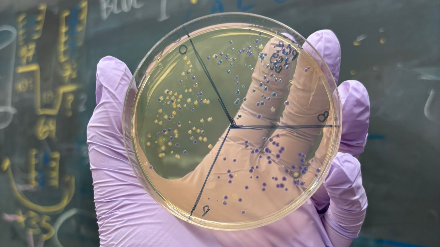
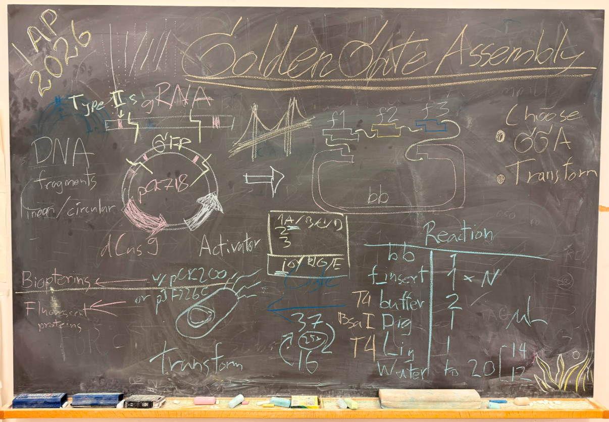
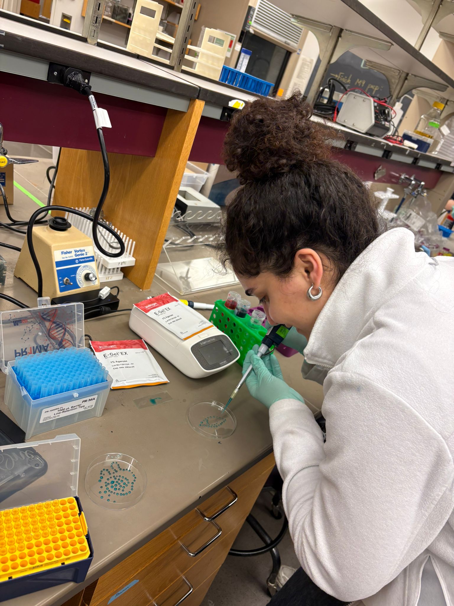
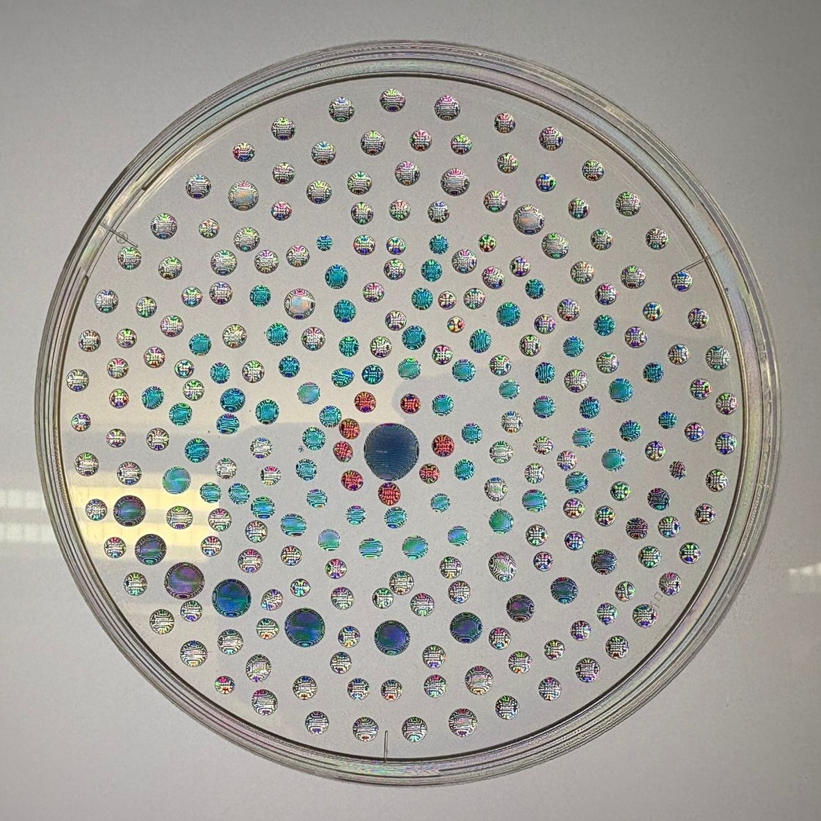
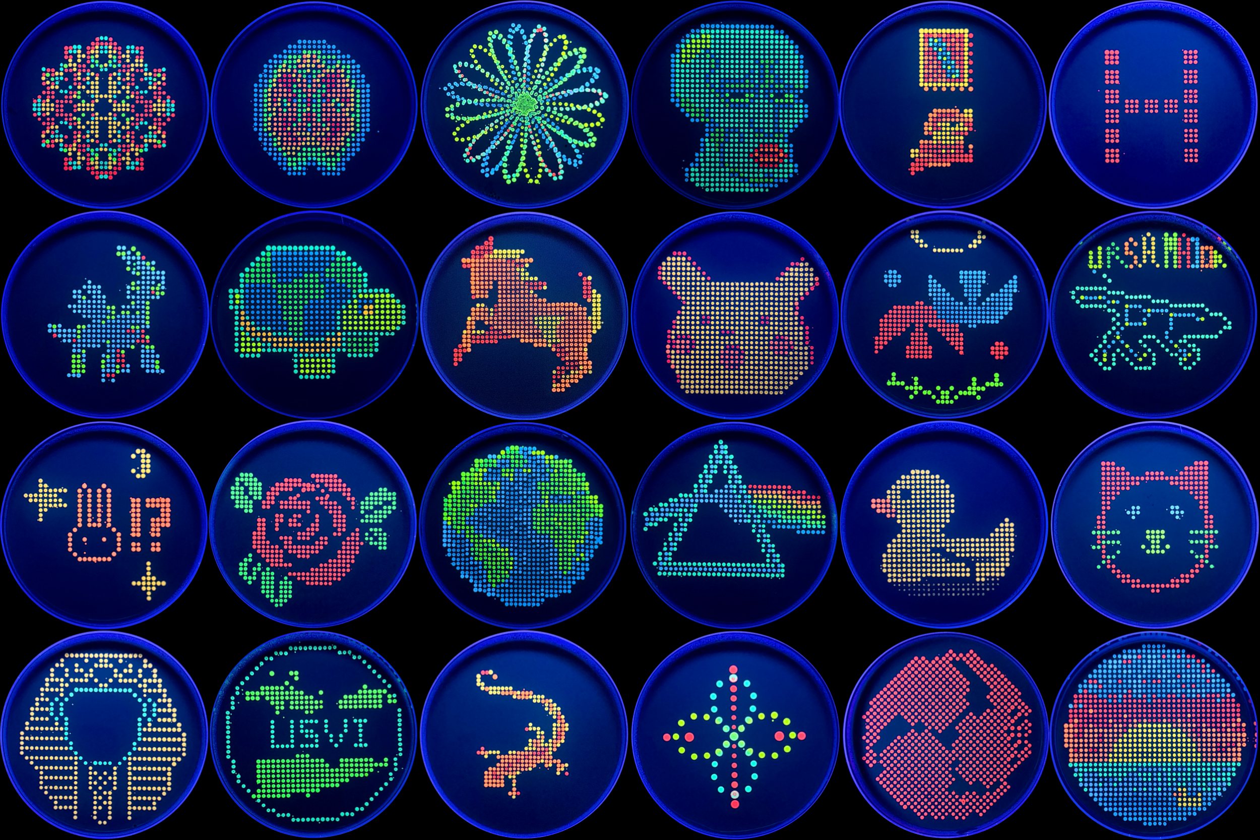
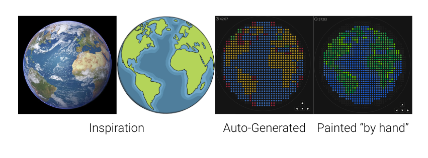
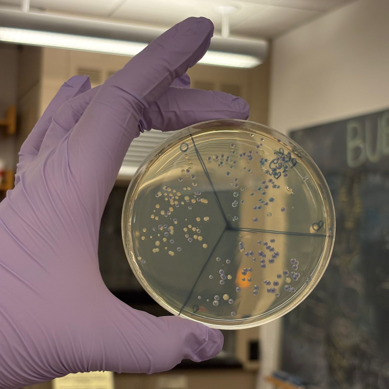
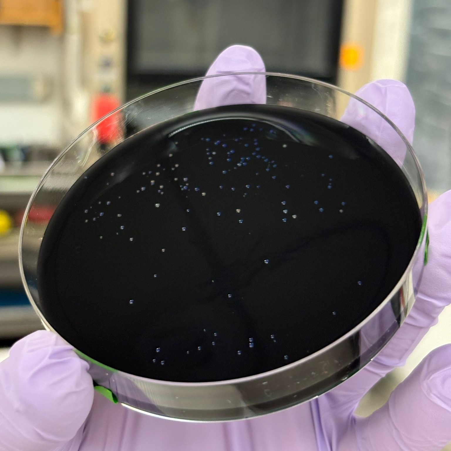
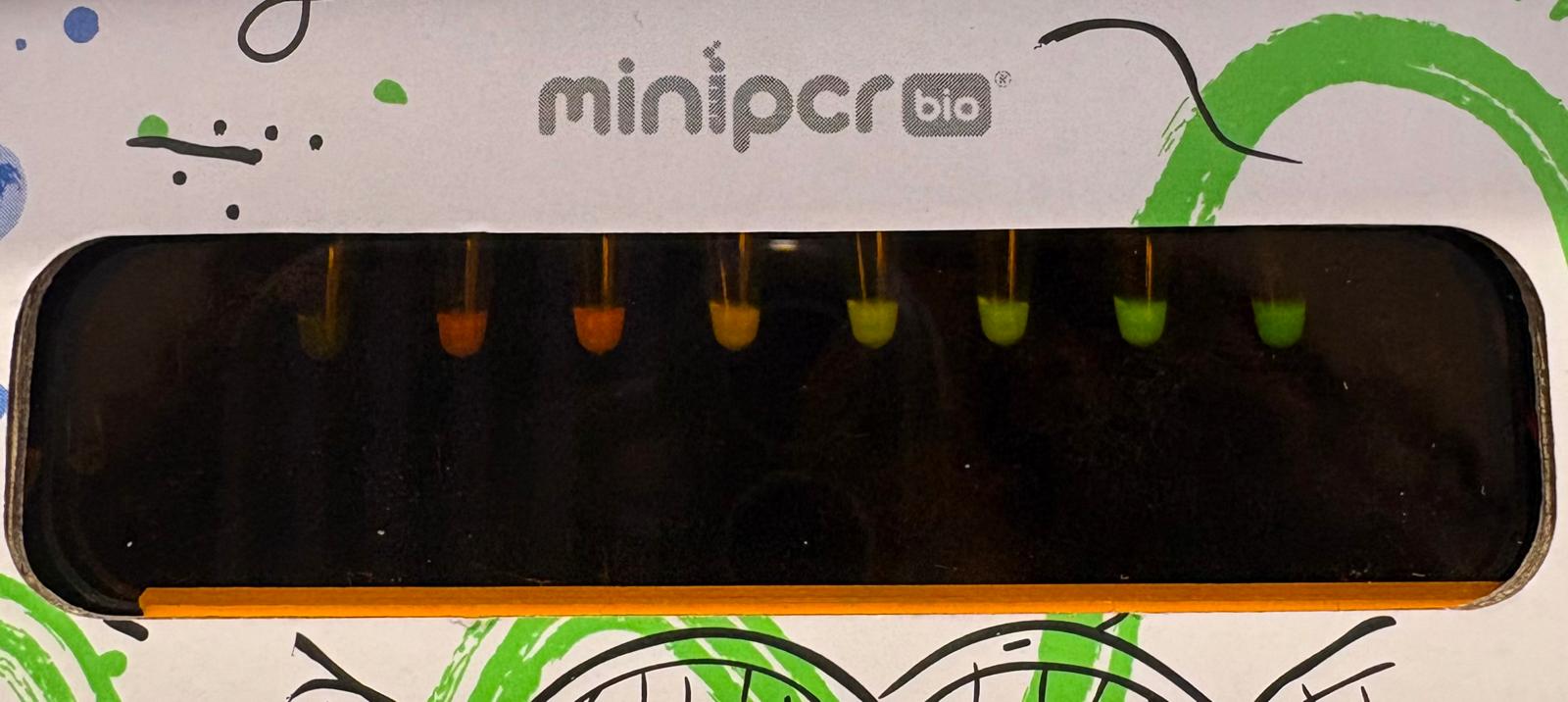
In this week’s lab, we used the Opentrons OT-2 pipetting robot and genetically engineered E. coli bacteria to create bio art on black (charcoal) agar plates! The bacteria were engineered to express fluorescent proteins (such as GFP – Green Fluorescent Protein), allowing them to glow in multiple colors under ultraviolet light.

*I mainly used the GUI at opentrons-art.rcdonovan.com to produce my designs due to the short notice before the lab.

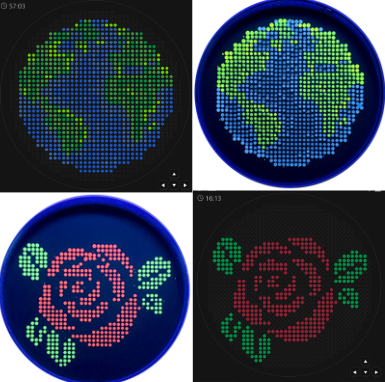
My first idea for this project was to create a picture of Earth that represents both the diverse backgrounds and countries students in the class and at MIT come from, and the global impact I hope to have through my work. I started by finding a reference photo and uploading it to the GUI. The result wasn’t very good, but I used it as a base and painted my final design over it. I would have loved to include some white (which we don’t have) for clouds, but I think it turned out amazing even without it.

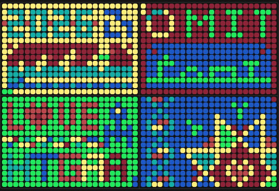
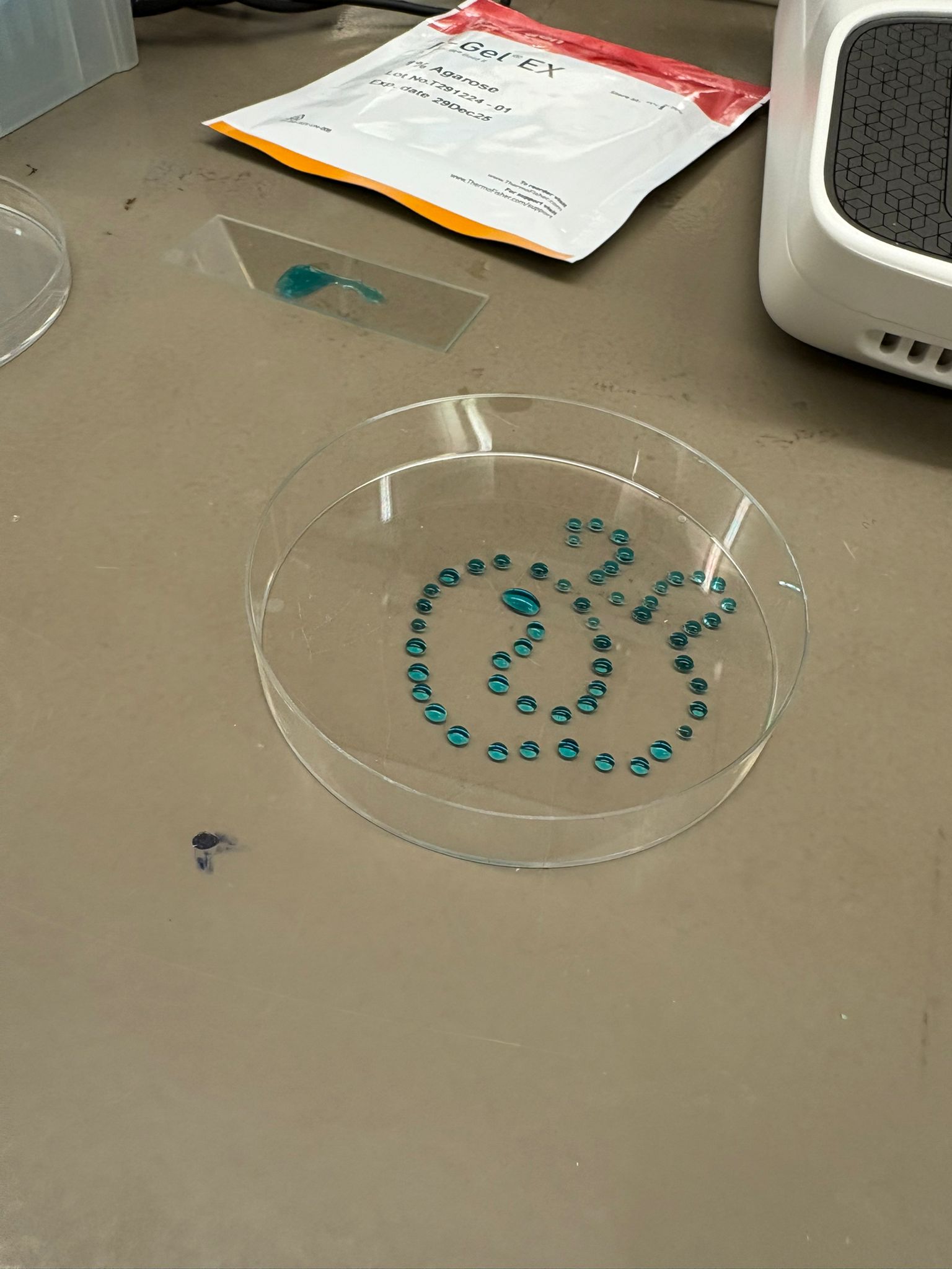
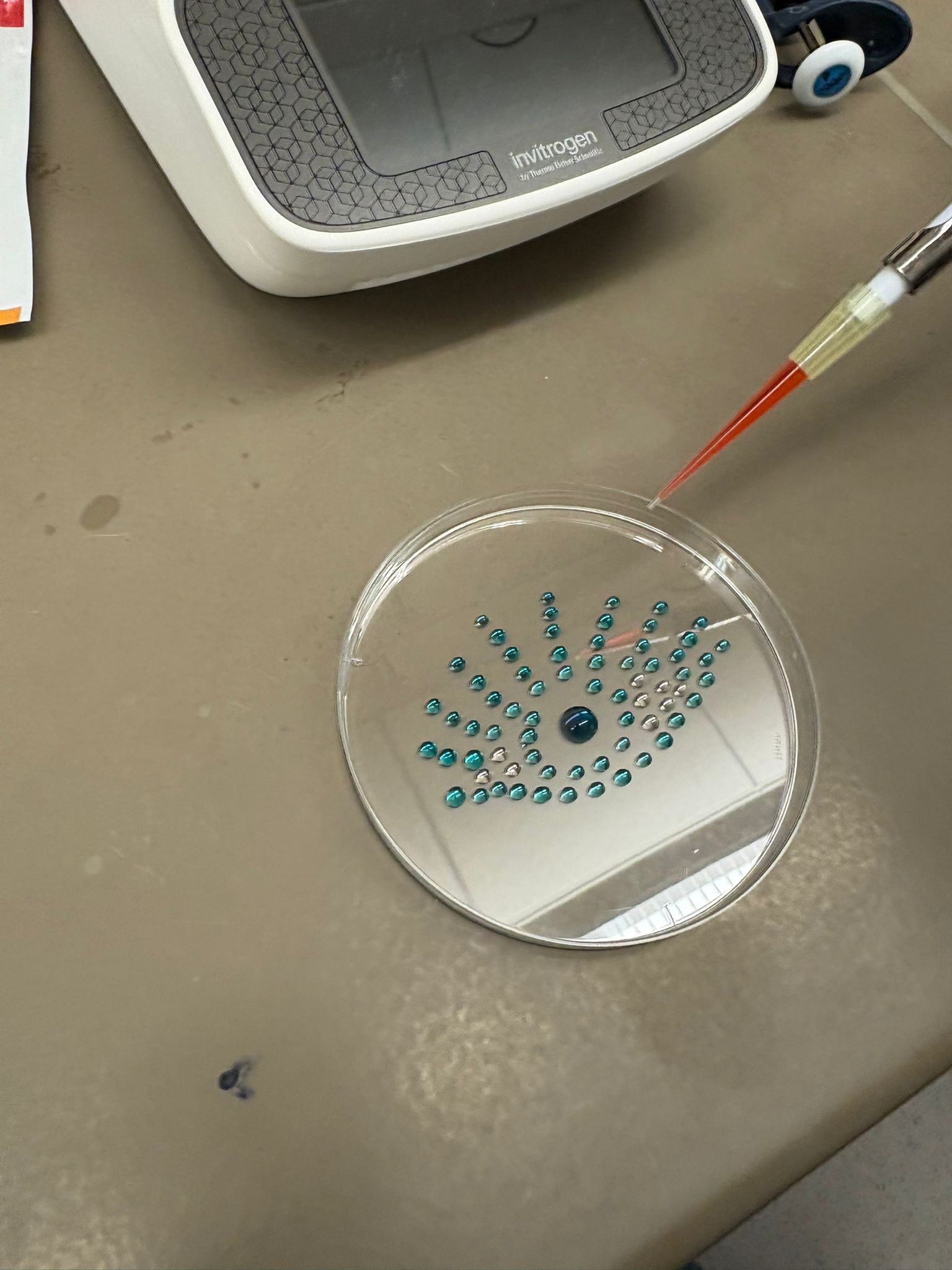
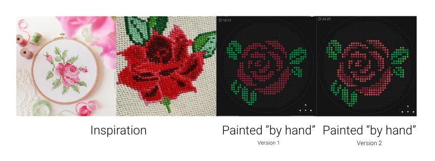
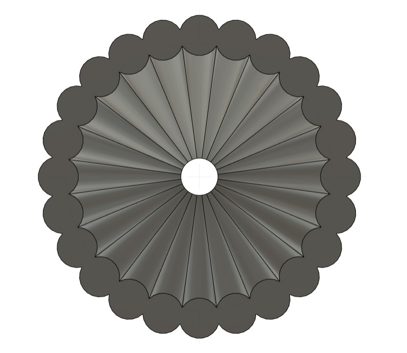
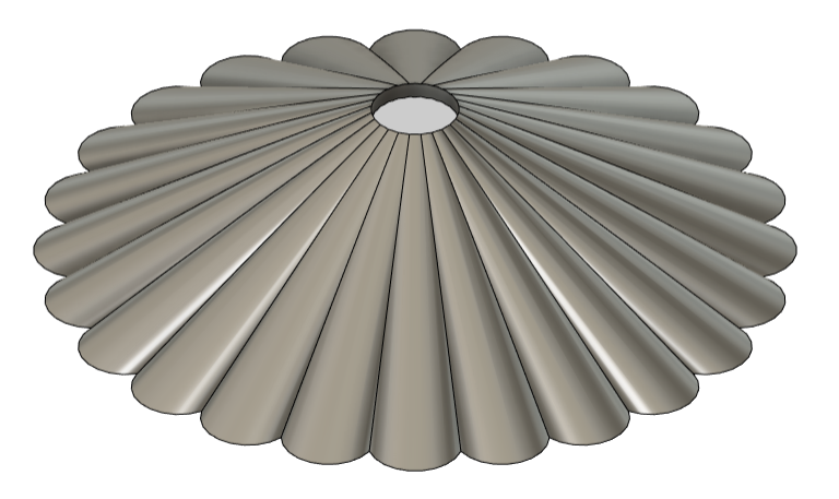
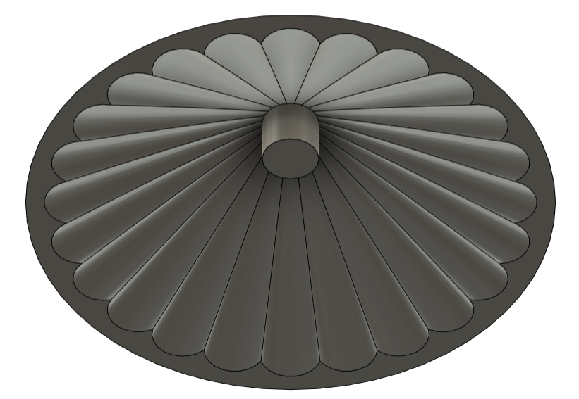
The “pixelated” look of the art examples from previous years reminded both me and my mother, who, among other things, is a textile designer, of cross-stitch embroidery. I wanted to create a design inspired by the classic rose cross patterns - but using this new, cutting-edge technology. A merge between the past and the future.

Here is my design process in images:

Here is my Python script for the Earth design:

from opentrons import types

import string

metadata = {
    'protocolName': '{YOUR NAME} - Opentrons Art - HTGAA',
    'author': 'HTGAA',
    'source': 'HTGAA 2026',
    'apiLevel': '2.20'
}

Z_VALUE_AGAR = 2.0
POINT_SIZE = 0.75

venus_points = [(-9,33), (5,33), (7,33), (9,33), (11,31), (13,31), (11,29), (-19,25), (-17,25), (1,25), (3,25), (15,25), (-21,23), (-19,23), (-7,23), (-5,23), (-21,21), (-19,21), (-5,21), (-31,19), (-29,19), (-21,19), (-19,19), (-17,19), (-15,19), (-11,19), (29,19), (-31,17), (-29,17), (-13,17), (-11,17), (29,17), (-13,15), (23,15), (-13,13), (11,13), (31,13), (33,13), (11,11), (31,11), (33,11), (-23,9), (-21,9), (11,9), (-33,3), (15,3), (-33,1), (17,1), (29,-3), (27,-5), (-17,-7), (-15,-7), (-13,-7), (23,-7), (25,-7), (27,-7), (-13,-9), (-11,-9), (23,-9), (-9,-11), (-7,-11), (23,-11), (-7,-13), (27,-13), (25,-15), (-5,-17), (-5,-19), (-7,-21)]
mwasabi_points = [(-7,33), (-5,33), (-3,33), (-9,31), (-7,31), (-3,31), (-1,31), (-17,29), (-15,29), (-5,29), (-1,29), (1,29), (21,29), (-19,27), (-17,27), (-15,27), (-13,27), (-5,27), (-3,27), (-1,27), (13,27), (19,27), (-21,25), (11,25), (17,25), (23,25), (17,23), (19,23), (25,23), (27,23), (27,21), (-27,19), (-13,19), (7,19), (13,19), (15,19), (19,19), (25,19), (7,17), (11,17), (-27,15), (-25,15), (-17,15), (13,15), (15,15), (17,15), (29,15), (-27,13), (-23,13), (23,13), (25,13), (-35,11), (-31,11), (-21,11), (-15,11), (-13,11), (23,11), (-35,9), (-31,9), (-27,9), (-25,9), (-19,9), (7,9), (25,9), (27,9), (29,9), (-35,7), (-33,7), (-29,7), (-27,7), (5,7), (11,7), (13,7), (15,7), (17,7), (19,7), (21,7), (23,7), (27,7), (29,7), (31,7), (-33,5), (-29,5), (-23,5), (5,5), (11,5), (13,5), (23,5), (27,5), (33,5), (-29,3), (5,3), (19,3), (23,3), (29,3), (-31,1), (-29,1), (5,1), (11,1), (13,1), (25,1), (-31,-1), (5,-1), (15,-1), (17,-1), (25,-1), (-23,-3), (7,-3), (9,-3), (11,-3), (17,-3), (21,-3), (25,-3), (-19,-5), (19,-5), (23,-5), (25,-5), (19,-7), (-17,-9), (-15,-9), (19,-9), (-23,-11), (-21,-11), (-15,-11), (-13,-11), (-11,-11), (19,-11), (-21,-13), (19,-13), (21,-13), (23,-13), (-17,-15), (19,-15), (27,-15), (-17,-17), (-7,-17), (19,-17), (-17,-19), (-15,-19), (-11,-19), (-7,-19), (19,-19), (-13,-21), (-11,-21), (-13,-23), (-9,-23), (-7,-23), (-15,-25), (-11,-25), (-9,-25)]
azurite_points = [(-1,33), (3,33), (-15,31), (-13,31), (1,31), (7,31), (9,31), (15,31), (-11,29), (-9,29), (-7,29), (3,29), (7,29), (9,29), (-11,27), (-7,27), (1,27), (3,27), (5,27), (9,27), (11,27), (-15,25), (-3,25), (-1,25), (5,25), (7,25), (9,25), (13,25), (-17,23), (-3,23), (-1,23), (1,23), (5,23), (7,23), (11,23), (-17,21), (-15,21), (-13,21), (-11,21), (-9,21), (-7,21), (-3,21), (-1,21), (1,21), (7,21), (9,21), (11,21), (-9,19), (-7,19), (-5,19), (-1,19), (5,19), (-9,17), (-7,17), (-3,17), (-1,17), (5,17), (-11,15), (-9,15), (-1,15), (1,15), (3,15), (5,15), (7,15), (25,15), (27,15), (-11,13), (-9,13), (1,13), (5,13), (7,13), (13,13), (17,13), (19,13), (21,13), (-11,11), (-9,11), (-1,11), (3,11), (5,11), (7,11), (9,11), (13,11), (15,11), (19,11), (21,11), (-17,9), (-15,9), (-13,9), (-11,9), (-9,9), (5,9), (-21,7), (-19,7), (-17,7), (-15,7), (-3,7), (1,7), (3,7), (-21,5), (-19,5), (-17,5), (1,5), (3,5), (-25,3), (-23,3), (-21,3), (-15,3), (-3,3), (-1,3), (1,3), (3,3), (31,3), (33,3), (-35,1), (-25,1), (-23,1), (-21,1), (1,1), (3,1), (29,1), (31,1), (-35,-1), (-33,-1), (-21,-1), (-19,-1), (-17,-1), (-5,-1), (3,-1), (29,-1), (31,-1), (-35,-3), (-33,-3), (-31,-3), (-27,-3), (-21,-3), (-19,-3), (-17,-3), (-15,-3), (-11,-3), (-3,-3), (3,-3), (5,-3), (31,-3), (-35,-5), (-33,-5), (-31,-5), (-29,-5), (-27,-5), (-17,-5), (-15,-5), (-13,-5), (3,-5), (5,-5), (7,-5), (9,-5), (11,-5), (29,-5), (31,-5), (-35,-7), (-33,-7), (-25,-7), (-11,-7), (-9,-7), (-7,-7), (5,-7), (7,-7), (9,-7), (11,-7), (13,-7), (29,-7), (-35,-9), (-33,-9), (-31,-9), (-25,-9), (-23,-9), (-9,-9), (-7,-9), (-5,-9), (-3,-9), (7,-9), (11,-9), (13,-9), (25,-9), (27,-9), (-25,-11), (-5,-11), (13,-11), (15,-11), (25,-11), (27,-11), (-25,-13), (-5,-13), (-3,-13), (1,-13), (13,-13), (15,-13), (25,-13), (29,-13), (-23,-15), (-3,-15), (1,-15), (13,-15), (15,-15), (23,-15), (29,-15), (-23,-17), (-21,-17), (-19,-17), (-3,-17), (1,-17), (13,-17), (15,-17), (23,-17), (25,-17), (-19,-19), (-3,-19), (13,-19), (15,-19), (23,-19), (-19,-21), (-17,-21), (-5,-21), (-3,-21), (-1,-21), (9,-21), (13,-21), (15,-21), (17,-21), (21,-21), (23,-21), (-27,-23), (-25,-23), (-17,-23), (15,-23), (17,-23), (-23,-25), (-17,-25), (-7,-25), (-5,-25), (-21,-27), (-19,-27), (-15,-27), (-9,-27), (-7,-27), (-21,-29), (-19,-29), (-15,-29), (-13,-29), (9,-29), (-15,-31), (-13,-31), (5,-31), (9,-31)]
electra2_points = [(-7,35), (-1,35), (1,35), (3,35), (5,35), (1,33), (3,31), (5,31), (5,29), (-9,27), (7,27), (-13,25), (-11,25), (-15,23), (-13,23), (-11,23), (3,23), (9,23), (3,21), (5,21), (-3,19), (1,19), (3,19), (-5,17), (1,17), (3,17), (-7,15), (-5,15), (-3,15), (-7,13), (-5,13), (-3,13), (-1,13), (3,13), (15,13), (-7,11), (-5,11), (-3,11), (1,11), (17,11), (-7,9), (-5,9), (-3,9), (-1,9), (1,9), (3,9), (-13,7), (-11,7), (-9,7), (-7,7), (-5,7), (-1,7), (-15,5), (-13,5), (-11,5), (-9,5), (-7,5), (-5,5), (-3,5), (-1,5), (-19,3), (-17,3), (-13,3), (-11,3), (-9,3), (-7,3), (-5,3), (35,3), (-19,1), (-17,1), (-15,1), (-13,1), (-11,1), (-9,1), (-7,1), (-5,1), (-3,1), (-1,1), (33,1), (35,1), (-15,-1), (-13,-1), (-11,-1), (-9,-1), (-7,-1), (-3,-1), (-1,-1), (1,-1), (33,-1), (35,-1), (-13,-3), (-9,-3), (-7,-3), (-5,-3), (-1,-3), (1,-3), (33,-3), (35,-3), (-11,-5), (-9,-5), (-7,-5), (-5,-5), (-3,-5), (-1,-5), (1,-5), (33,-5), (35,-5), (-31,-7), (-29,-7), (-27,-7), (-5,-7), (-3,-7), (-1,-7), (1,-7), (3,-7), (31,-7), (33,-7), (35,-7), (-29,-9), (-27,-9), (-1,-9), (1,-9), (3,-9), (5,-9), (9,-9), (29,-9), (31,-9), (33,-9), (-33,-11), (-31,-11), (-29,-11), (-27,-11), (-3,-11), (-1,-11), (1,-11), (3,-11), (5,-11), (7,-11), (9,-11), (11,-11), (29,-11), (31,-11), (-33,-13), (-31,-13), (-29,-13), (-27,-13), (-1,-13), (3,-13), (5,-13), (7,-13), (9,-13), (11,-13), (31,-13), (-31,-15), (-29,-15), (-27,-15), (-25,-15), (-1,-15), (3,-15), (5,-15), (7,-15), (9,-15), (11,-15), (-31,-17), (-29,-17), (-27,-17), (-25,-17), (-1,-17), (3,-17), (5,-17), (7,-17), (9,-17), (11,-17), (27,-17), (29,-17), (-29,-19), (-27,-19), (-25,-19), (-23,-19), (-21,-19), (-1,-19), (1,-19), (3,-19), (5,-19), (7,-19), (9,-19), (11,-19), (25,-19), (27,-19), (29,-19), (-27,-21), (-25,-21), (-23,-21), (-21,-21), (1,-21), (3,-21), (5,-21), (7,-21), (11,-21), (25,-21), (27,-21), (-23,-23), (-21,-23), (-19,-23), (-5,-23), (-3,-23), (-1,-23), (1,-23), (3,-23), (5,-23), (7,-23), (9,-23), (11,-23), (13,-23), (19,-23), (21,-23), (23,-23), (25,-23), (27,-23), (-21,-25), (-19,-25), (-3,-25), (-1,-25), (1,-25), (3,-25), (5,-25), (7,-25), (9,-25), (11,-25), (13,-25), (15,-25), (17,-25), (19,-25), (21,-25), (23,-25), (-17,-27), (-11,-27), (-5,-27), (-3,-27), (-1,-27), (1,-27), (3,-27), (5,-27), (7,-27), (9,-27), (11,-27), (13,-27), (15,-27), (17,-27), (19,-27), (21,-27), (-17,-29), (-11,-29), (-9,-29), (-7,-29), (-5,-29), (-3,-29), (-1,-29), (1,-29), (3,-29), (5,-29), (7,-29), (11,-29), (13,-29), (15,-29), (17,-29), (19,-29), (21,-29), (-11,-31), (-9,-31), (-7,-31), (-5,-31), (-3,-31), (-1,-31), (1,-31), (3,-31), (7,-31), (11,-31), (13,-31), (15,-31), (-9,-33), (-7,-33), (-5,-33), (-3,-33), (-1,-33), (1,-33), (3,-33), (5,-33), (7,-33), (9,-33), (-7,-35), (-5,-35), (-3,-35), (-1,-35), (1,-35), (3,-35), (5,-35), (7,-35)]
mclover3_points = [(-5,35), (-3,35), (-11,31), (-5,31), (-21,29), (-19,29), (-13,29), (-3,29), (13,29), (15,29), (17,29), (19,29), (-21,27), (15,27), (17,27), (21,27), (-23,25), (-9,25), (-7,25), (-5,25), (19,25), (21,25), (-27,23), (-25,23), (-23,23), (-9,23), (13,23), (15,23), (21,23), (23,23), (-27,21), (-25,21), (-23,21), (13,21), (15,21), (17,21), (19,21), (21,21), (23,21), (25,21), (-25,19), (-23,19), (9,19), (11,19), (17,19), (21,19), (23,19), (27,19), (-27,17), (-25,17), (-23,17), (-21,17), (-19,17), (-17,17), (-15,17), (9,17), (13,17), (15,17), (17,17), (19,17), (21,17), (23,17), (25,17), (27,17), (-31,15), (-29,15), (-23,15), (-21,15), (-19,15), (-15,15), (9,15), (11,15), (19,15), (21,15), (-33,13), (-31,13), (-29,13), (-25,13), (-21,13), (-19,13), (-17,13), (-15,13), (9,13), (27,13), (29,13), (-33,11), (-29,11), (-27,11), (-25,11), (-23,11), (-19,11), (-17,11), (25,11), (27,11), (29,11), (-33,9), (-29,9), (9,9), (13,9), (15,9), (17,9), (19,9), (21,9), (23,9), (31,9), (33,9), (35,9), (-31,7), (-25,7), (-23,7), (7,7), (9,7), (25,7), (33,7), (35,7), (-35,5), (-31,5), (-27,5), (-25,5), (7,5), (9,5), (15,5), (17,5), (19,5), (21,5), (25,5), (29,5), (31,5), (35,5), (-35,3), (-31,3), (-27,3), (7,3), (9,3), (11,3), (13,3), (17,3), (21,3), (25,3), (27,3), (-27,1), (7,1), (9,1), (15,1), (19,1), (21,1), (23,1), (27,1), (-29,-1), (-27,-1), (-25,-1), (-23,-1), (7,-1), (9,-1), (11,-1), (13,-1), (19,-1), (21,-1), (23,-1), (27,-1), (-29,-3), (-25,-3), (13,-3), (15,-3), (19,-3), (23,-3), (27,-3), (-25,-5), (-23,-5), (-21,-5), (13,-5), (15,-5), (17,-5), (21,-5), (-23,-7), (-21,-7), (-19,-7), (15,-7), (17,-7), (21,-7), (-21,-9), (-19,-9), (15,-9), (17,-9), (21,-9), (-19,-11), (-17,-11), (17,-11), (21,-11), (-19,-13), (-17,-13), (-15,-13), (-13,-13), (-11,-13), (-9,-13), (17,-13), (-21,-15), (-19,-15), (-15,-15), (-13,-15), (-11,-15), (-9,-15), (-7,-15), (-5,-15), (17,-15), (21,-15), (-15,-17), (-13,-17), (-11,-17), (-9,-17), (17,-17), (21,-17), (-13,-19), (-9,-19), (17,-19), (21,-19), (-15,-21), (-9,-21), (19,-21), (-15,-23), (-11,-23), (-13,-25), (-13,-27)]
mjuniper_points = [(-23,-13)]

point_name_pairing = [("venus", venus_points),("mwasabi", mwasabi_points),("azurite", azurite_points),("electra2", electra2_points),("mclover3", mclover3_points),("mjuniper", mjuniper_points)]

# Robot deck setup constants
TIP_RACK_DECK_SLOT = 9
COLORS_DECK_SLOT = 6
AGAR_DECK_SLOT = 5
PIPETTE_STARTING_TIP_WELL = 'A1'

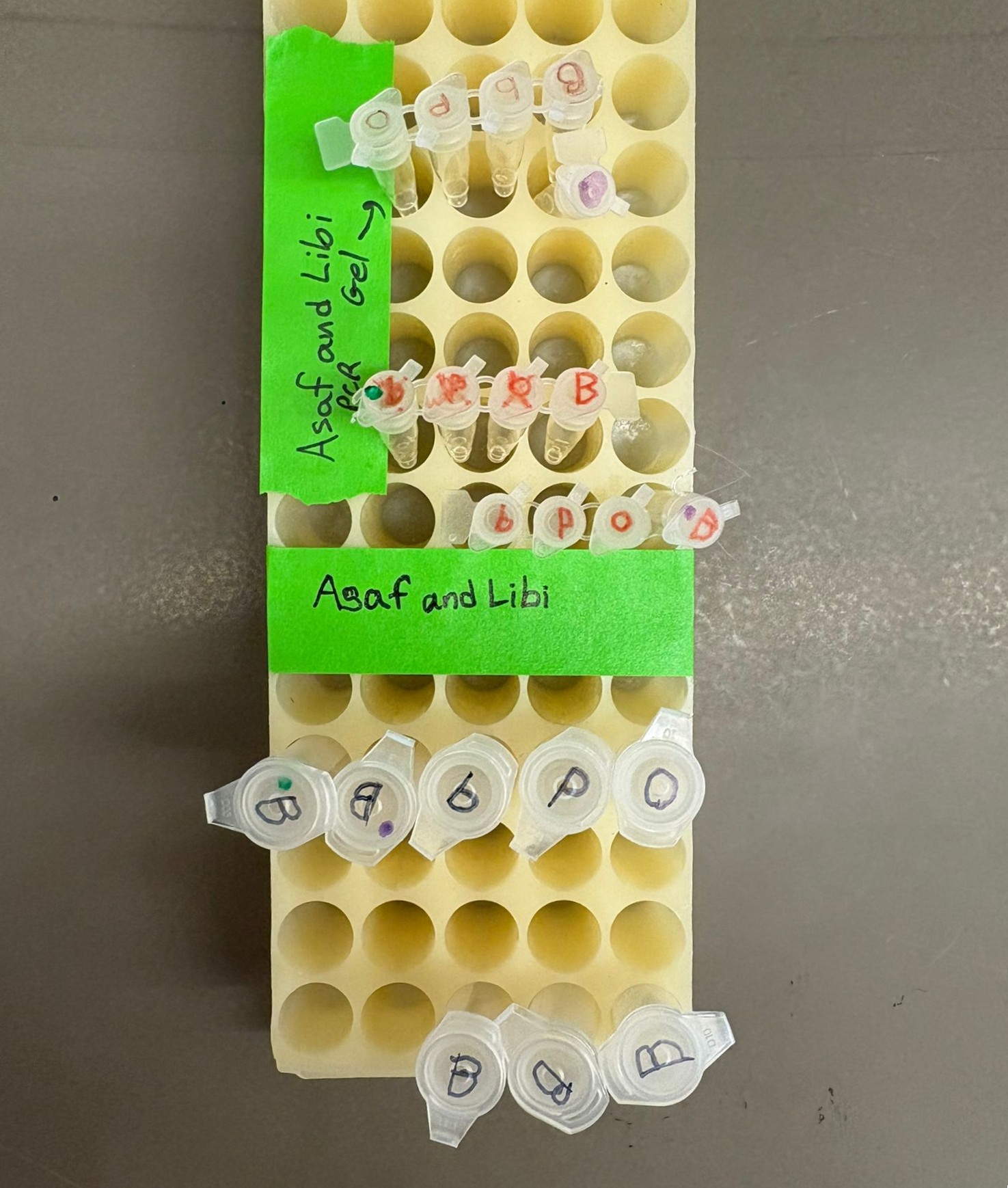
# Place the PCR tubes in this order
well_colors = {
    'A1': 'sfGFP',
    'A2': 'mRFP1',
    'A3': 'mKO2',
    'A4': 'Venus',
    'A5': 'mKate2_TF',
    'A6': 'Azurite',
    'A7': 'mCerulean3',
    'A8': 'mClover3',
    'A9': 'mJuniper',
    'A10': 'mTurquoise2',
    'A11': 'mBanana',
    'A12': 'mPlum',
    'B1': 'Electra2',
    'B2': 'mWasabi',
    'B3': 'mScarlet_I',
    'B4': 'mPapaya',
    'B5': 'eqFP578',
    'B6': 'tdTomato',
    'B7': 'DsRed',
    'B8': 'mKate2',
    'B9': 'EGFP',
    'B10': 'mRuby2',
    'B11': 'TagBFP',
    'B12': 'mChartreuse_TF',
    'C1': 'mLychee_TF',
    'C2': 'mTagBFP2',
    'C3': 'mEGFP',
    'C4': 'mNeonGreen',
    'C5': 'mAzamiGreen',
    'C6': 'mWatermelon',
    'C7': 'avGFP',
    'C8': 'mCitrine',
    'C9': 'mVenus',
    'C10': 'mCherry',
    'C11': 'mHoneydew',
    'C12': 'TagRFP',
    'D1': 'mTFP1',
    'D2': 'Ultramarine',
    'D3': 'ZsGreen1',
    'D4': 'mMiCy',
    'D5': 'mStayGold2',
    'D6': 'PA_GFP'
}

volume_used = {
    'venus': 0,
    'mwasabi': 0,
    'azurite': 0,
    'electra2': 0,
    'mclover3': 0,
    'mjuniper': 0
}

def update_volume_remaining(current_color, quantity_to_aspirate):
    rows = string.ascii_uppercase
    for well, color in list(well_colors.items()):
        if color == current_color:
            if (volume_used[current_color] + quantity_to_aspirate) > 250:
                # Move to next well horizontally by advancing row letter, keeping column number
                row = well[0]
                col = well[1:]
                
                # Find next row letter
                next_row = rows[rows.index(row) + 1]
                next_well = f"{next_row}{col}"
                
                del well_colors[well]
                well_colors[next_well] = current_color
                volume_used[current_color] = quantity_to_aspirate
            else:
                volume_used[current_color] += quantity_to_aspirate
            break

def run(protocol):
    # Load labware, modules and pipettes
    protocol.home()

    # Tips
    tips_20ul = protocol.load_labware('opentrons_96_tiprack_20ul', TIP_RACK_DECK_SLOT, 'Opentrons 20uL Tips')

    # Pipettes
    pipette_20ul = protocol.load_instrument("p20_single_gen2", "right", [tips_20ul])

    # Deep Well Plate
    temperature_plate = protocol.load_labware('nest_96_wellplate_2ml_deep', 6)

    # Agar Plate
    agar_plate = protocol.load_labware('htgaa_agar_plate', AGAR_DECK_SLOT, 'Agar Plate')
    agar_plate.set_offset(x=0.00, y=0.00, z=Z_VALUE_AGAR)

    # Get the top-center of the plate, make sure the plate was calibrated before running this
    center_location = agar_plate['A1'].top()

    pipette_20ul.starting_tip = tips_20ul.well(PIPETTE_STARTING_TIP_WELL)
    
    # Helper function (dispensing)
    def dispense_and_jog(pipette, volume, location):
        assert(isinstance(volume, (int, float)))
        # Go above the location
        above_location = location.move(types.Point(z=location.point.z + 2))
        pipette.move_to(above_location)
        # Go downwards and dispense
        pipette.dispense(volume, location)
        # Go upwards to avoid smearing
        pipette.move_to(above_location)

    # Helper function (color location)
    def location_of_color(color_string):
        for well,color in well_colors.items():
            if color.lower() == color_string.lower():
                return temperature_plate[well]
        raise ValueError(f"No well found with color {color_string}")

    # Print pattern by iterating over lists
    for i, (current_color, point_list) in enumerate(point_name_pairing):
        # Skip the rest of the loop if the list is empty
        if not point_list:
            continue

        # Get the tip for this run, set the bacteria color, and the aspirate bacteria of choice
        pipette_20ul.pick_up_tip()
        max_aspirate = int(18 // POINT_SIZE) * POINT_SIZE
        quantity_to_aspirate = min(len(point_list)*POINT_SIZE, max_aspirate)
        update_volume_remaining(current_color, quantity_to_aspirate)
        pipette_20ul.aspirate(quantity_to_aspirate, location_of_color(current_color))

        # Iterate over the current points list and dispense them, refilling along the way
        for i in range(len(point_list)):
            x, y = point_list[i]
            adjusted_location = center_location.move(types.Point(x, y))

            dispense_and_jog(pipette_20ul, POINT_SIZE, adjusted_location)
            
            if pipette_20ul.current_volume == 0 and len(point_list[i+1:]) > 0:
                quantity_to_aspirate = min(len(point_list[i:])*POINT_SIZE, max_aspirate)
                update_volume_remaining(current_color, quantity_to_aspirate)
                pipette_20ul.aspirate(quantity_to_aspirate, location_of_color(current_color))

        # Drop tip between each color
        pipette_20ul.drop_tip()

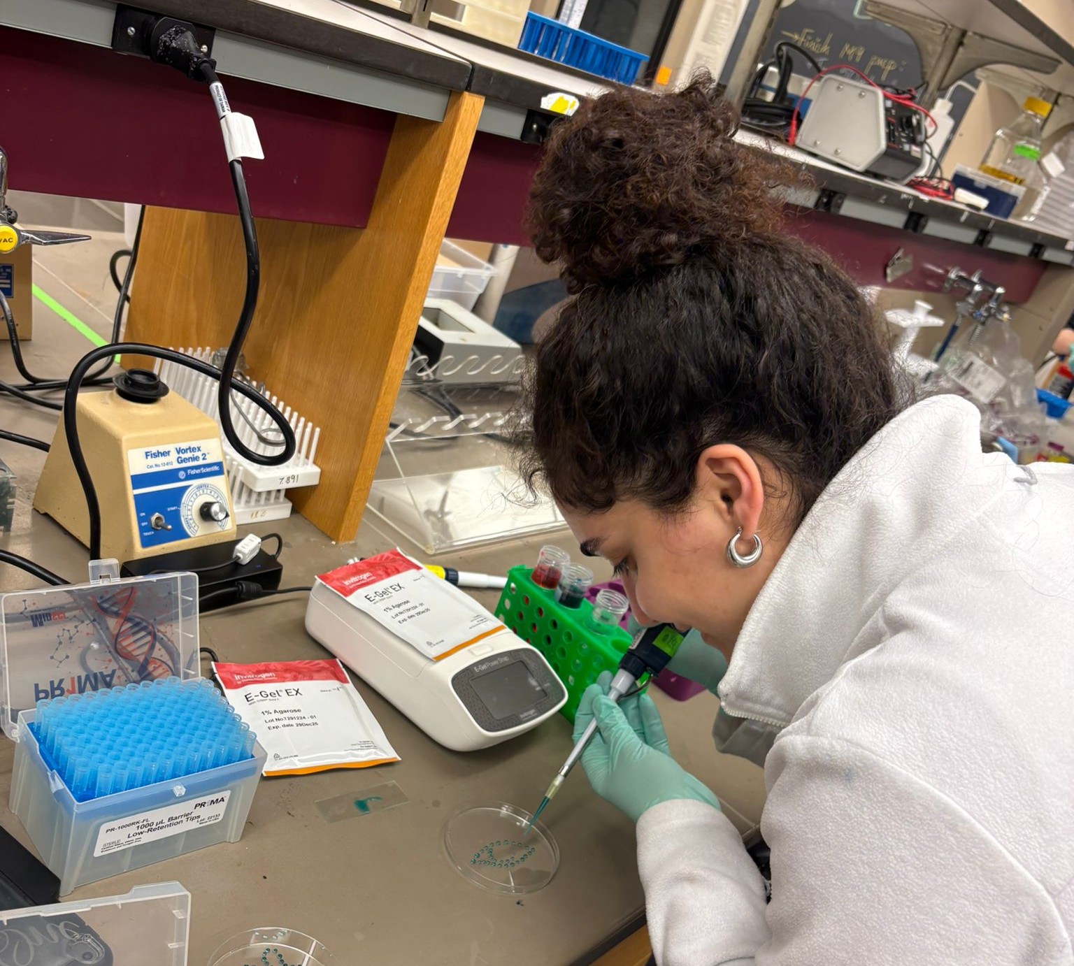
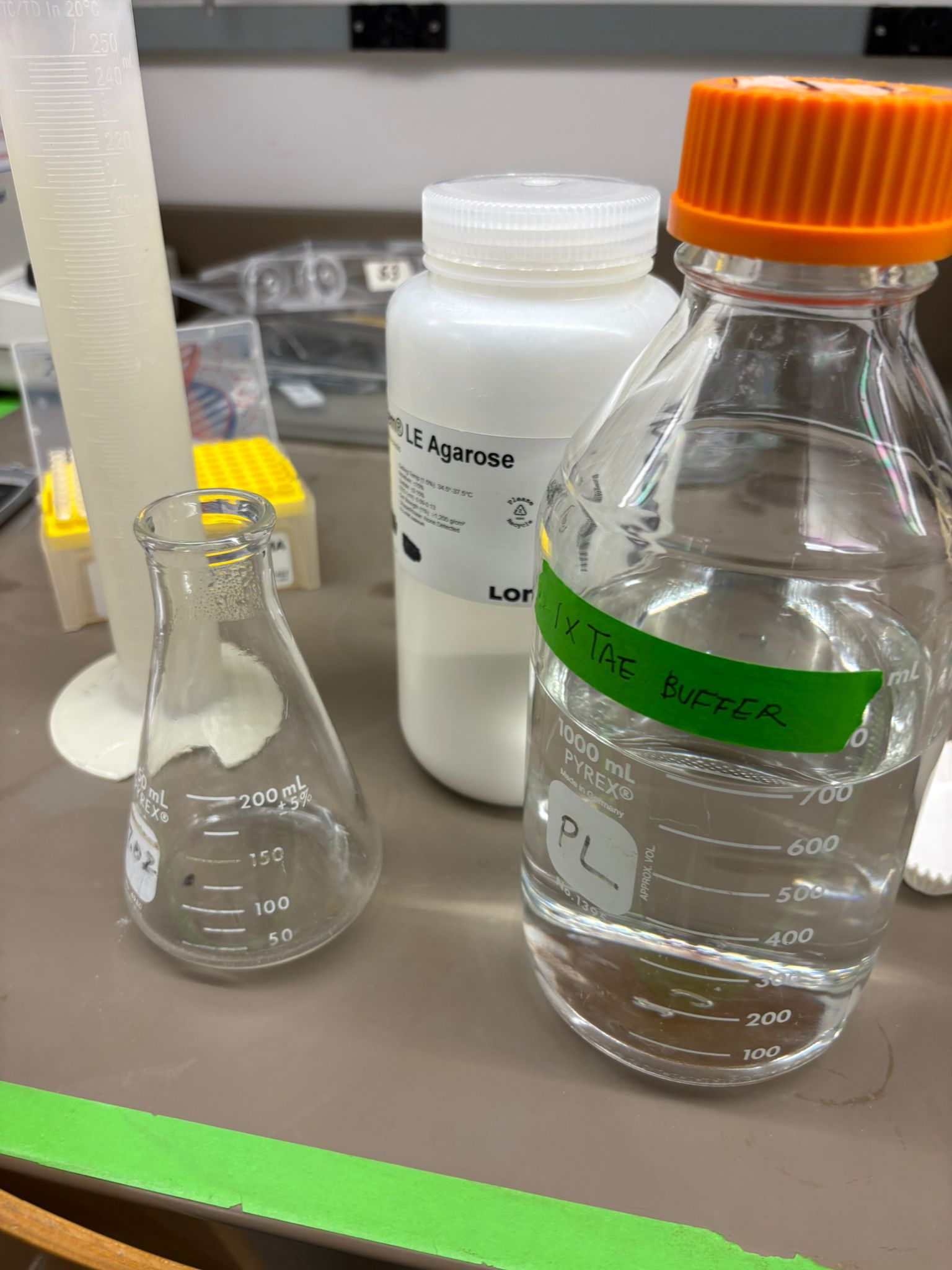
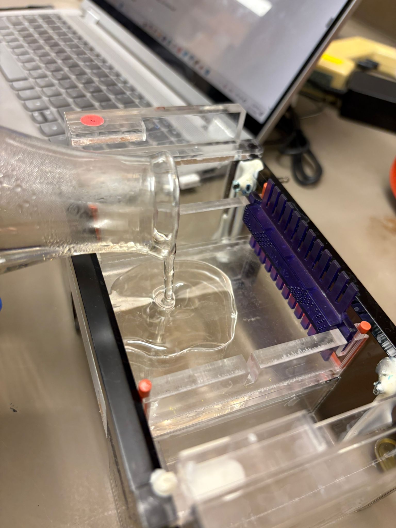
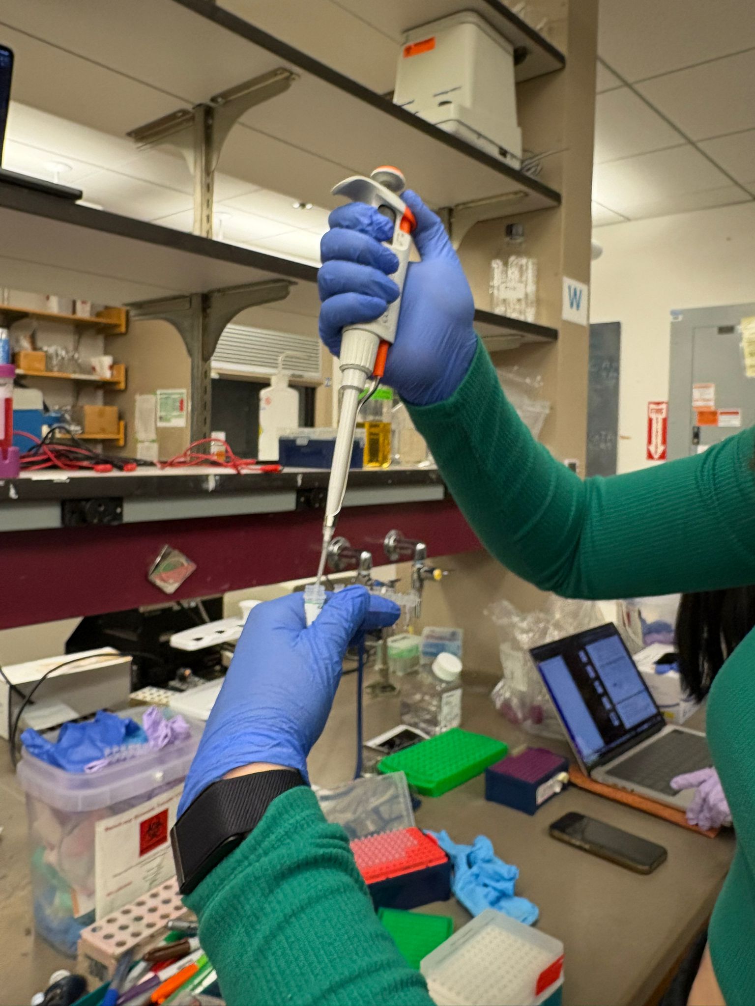
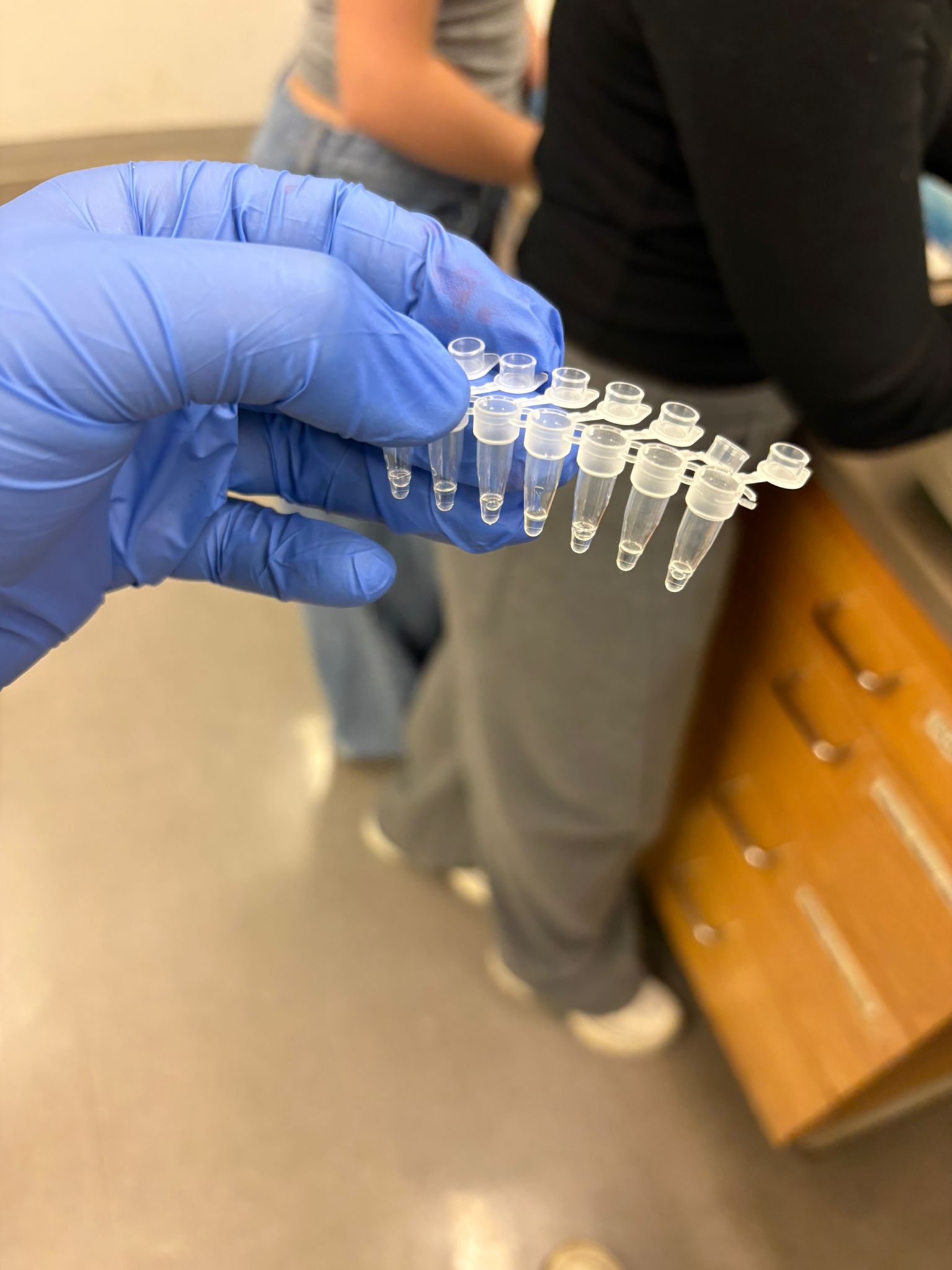
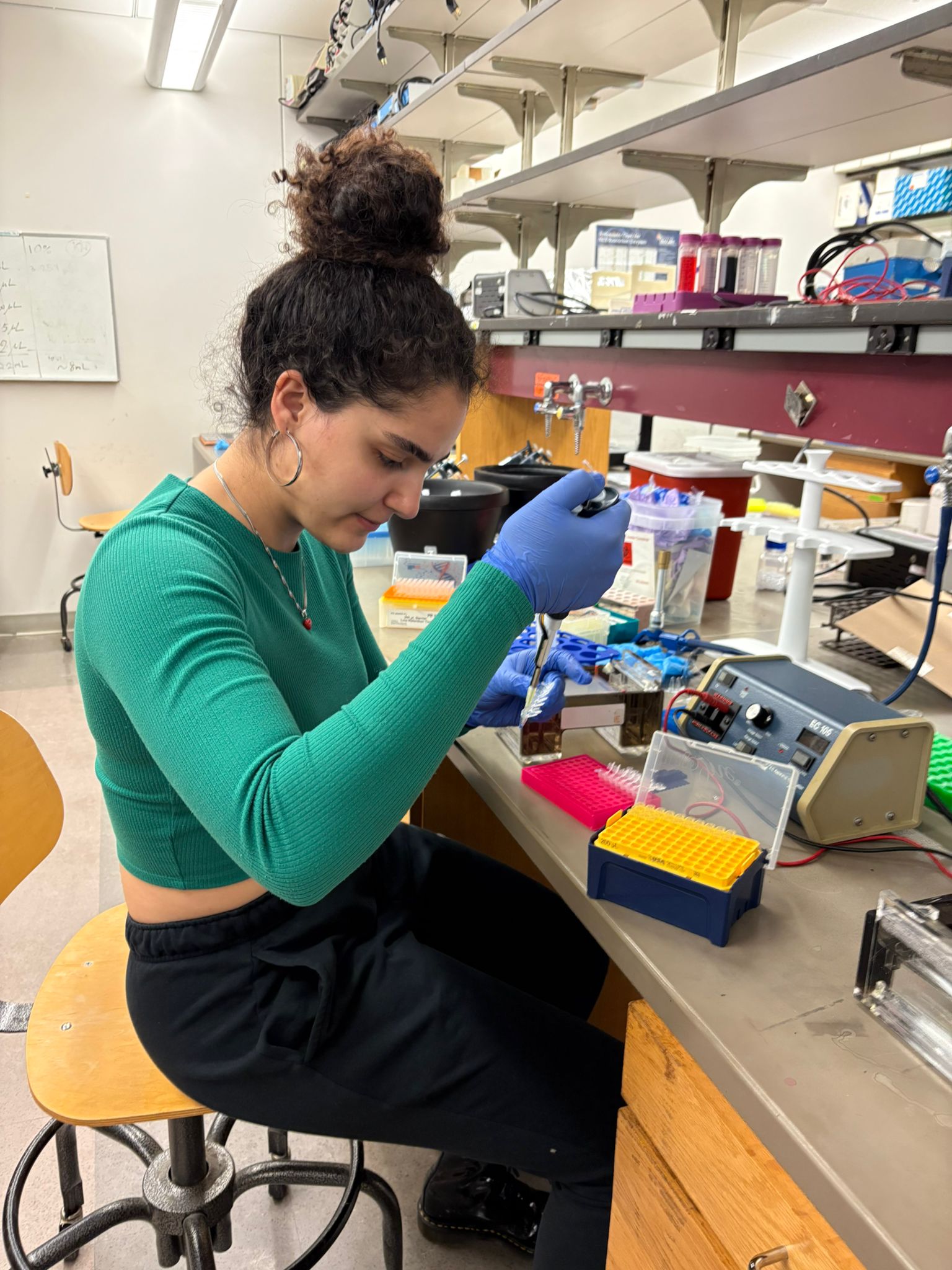
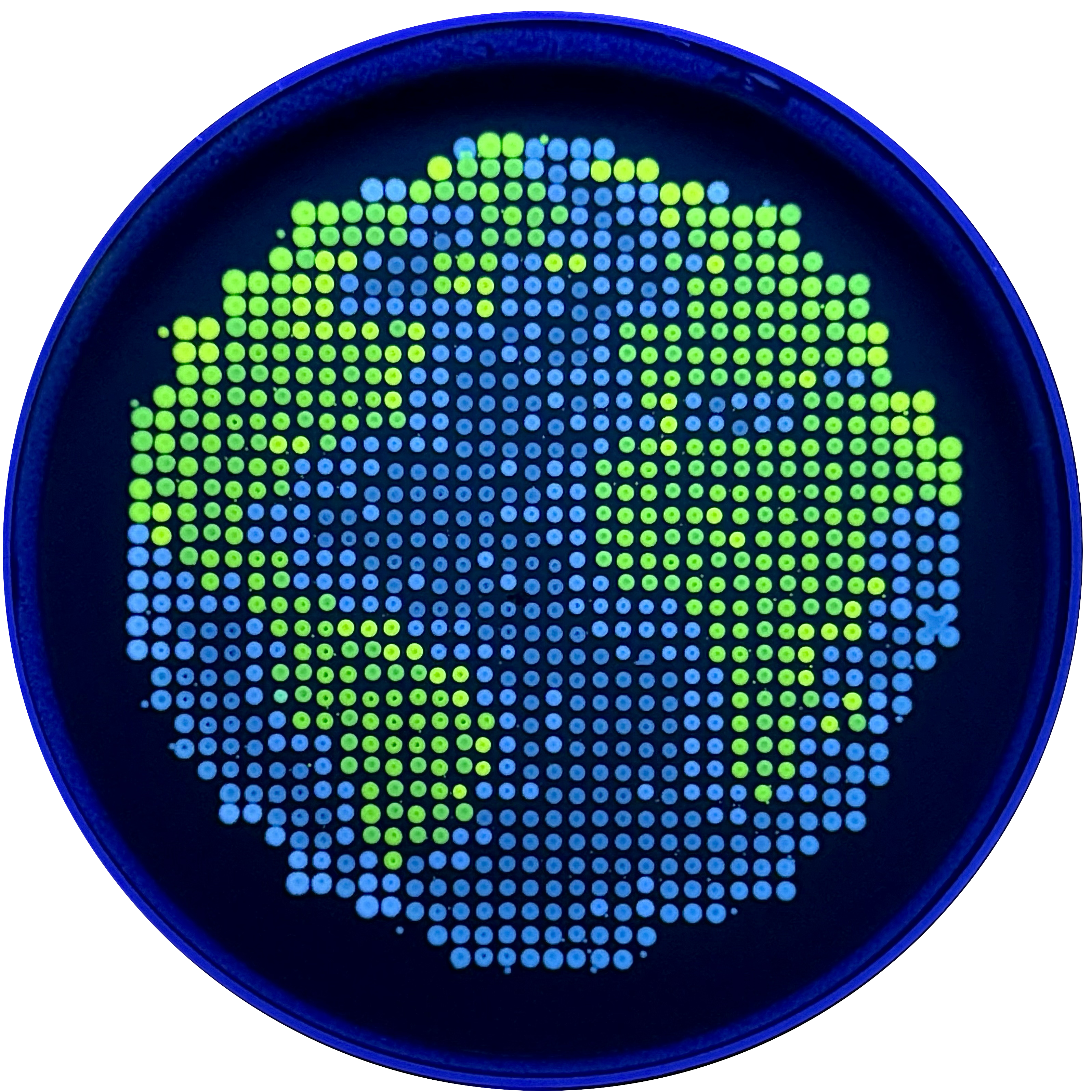
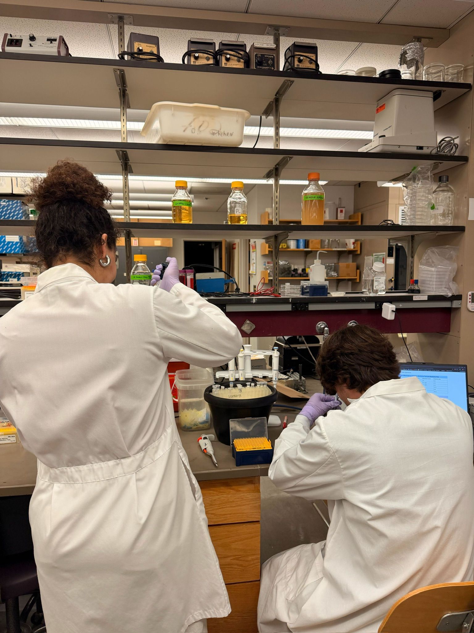
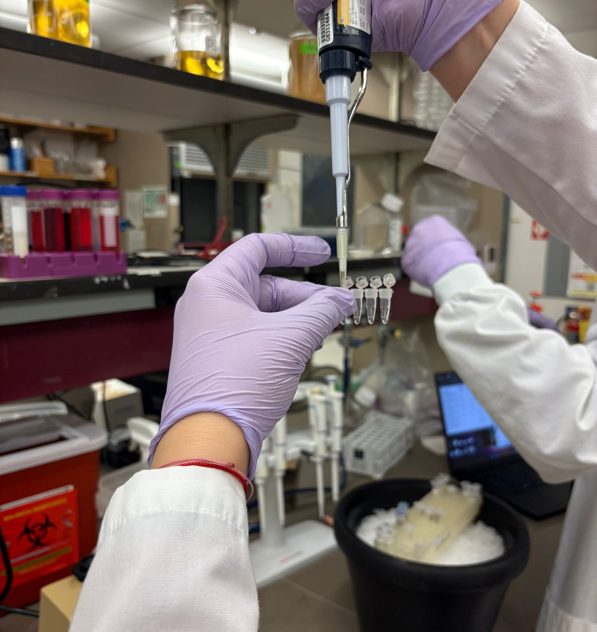
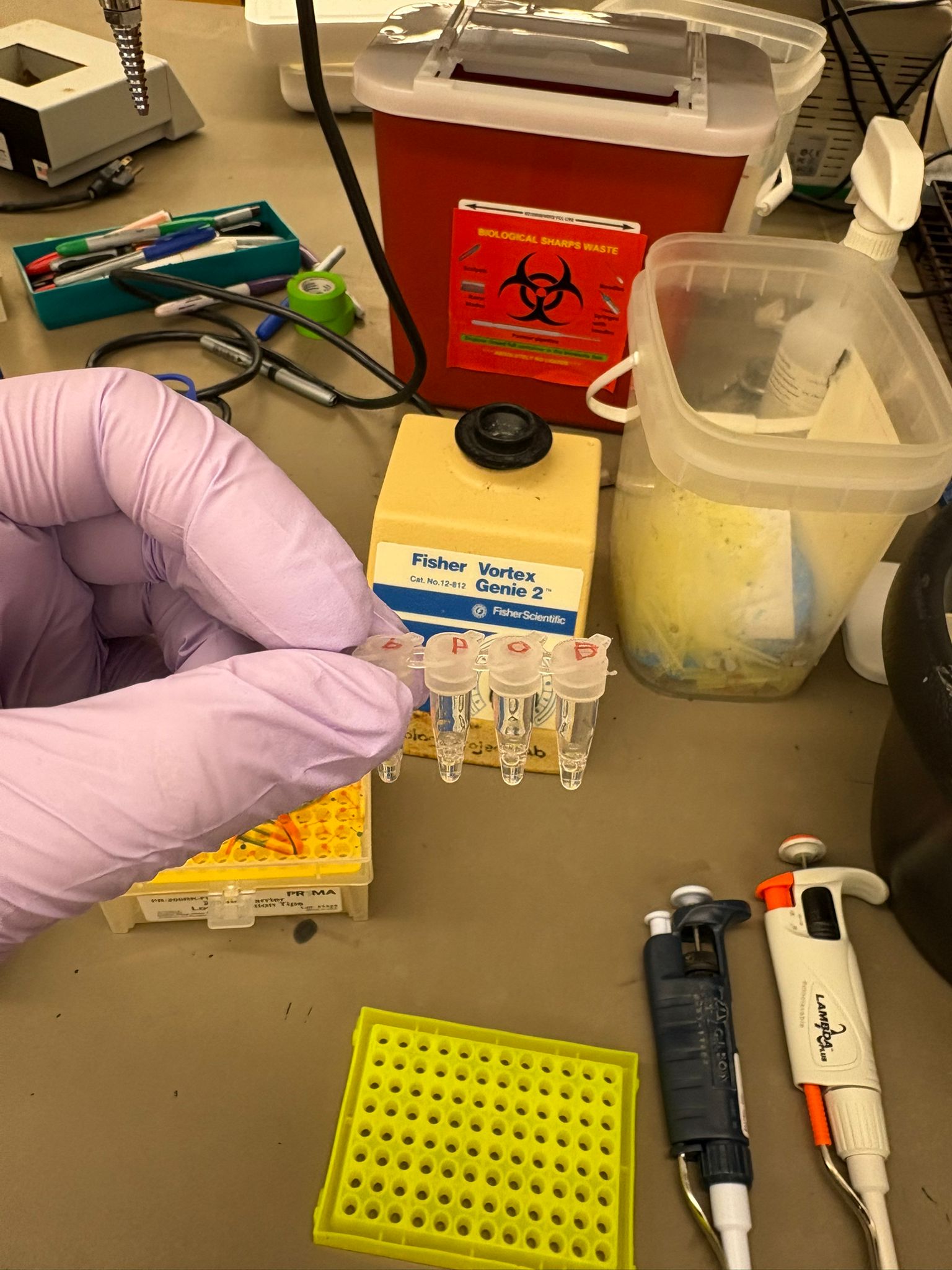
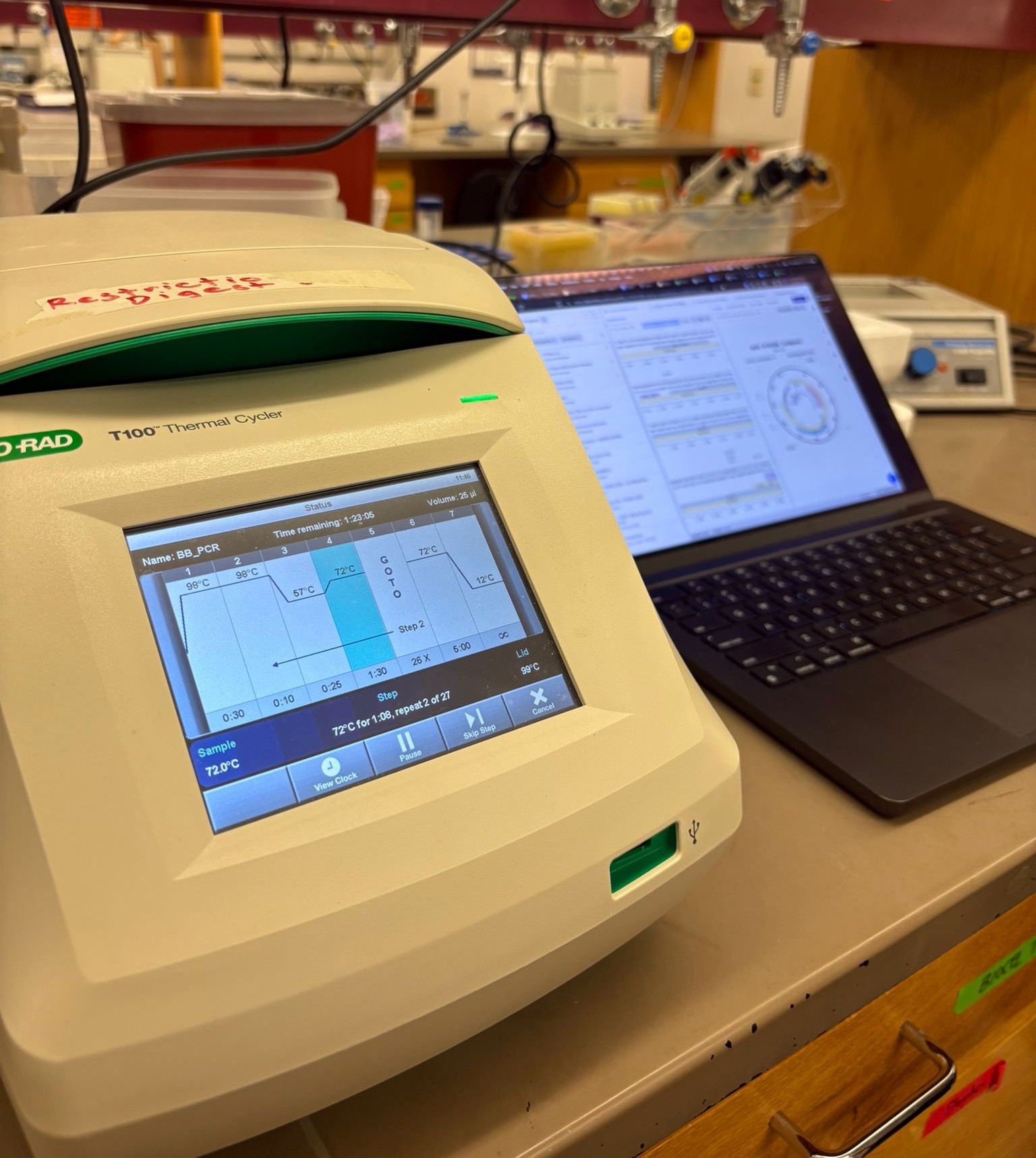
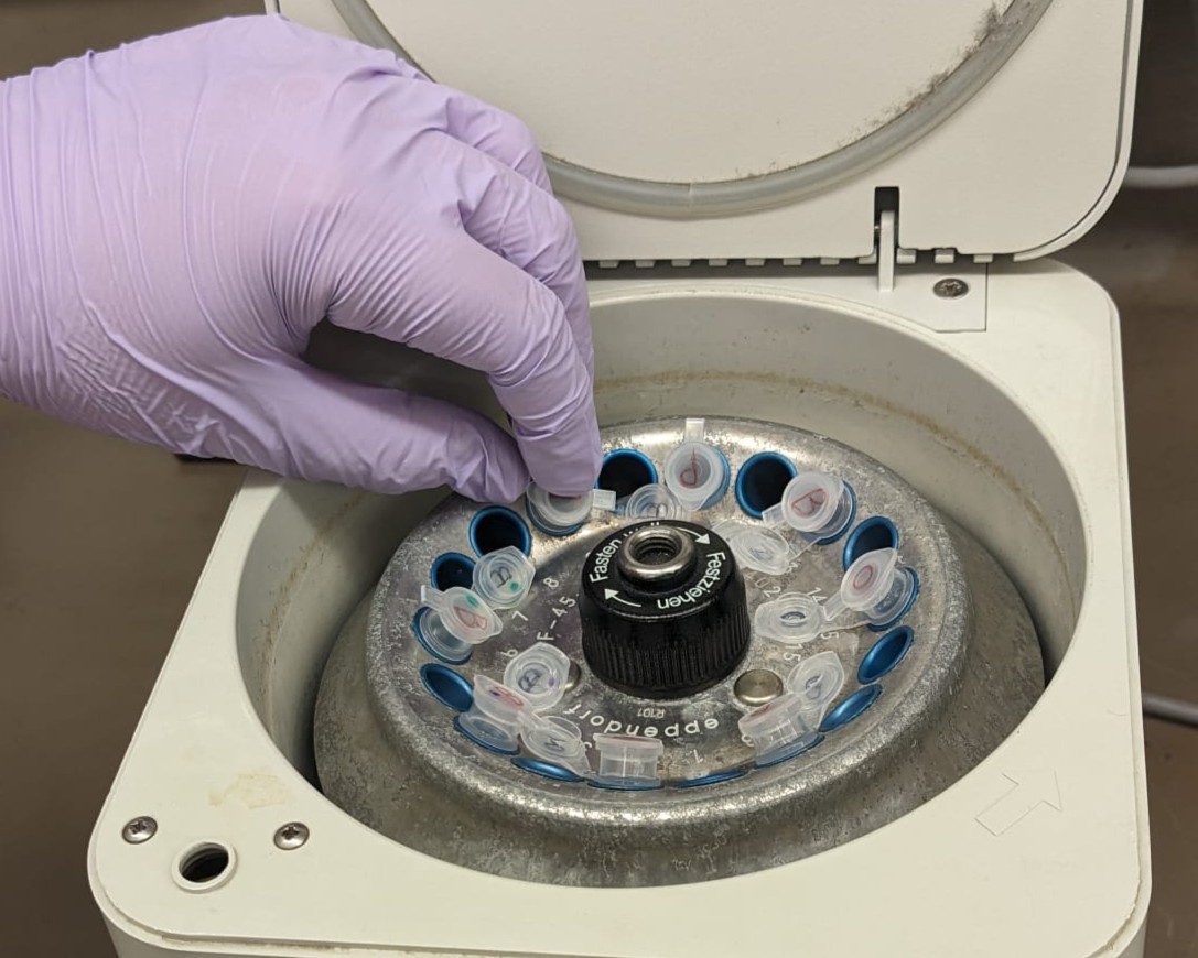
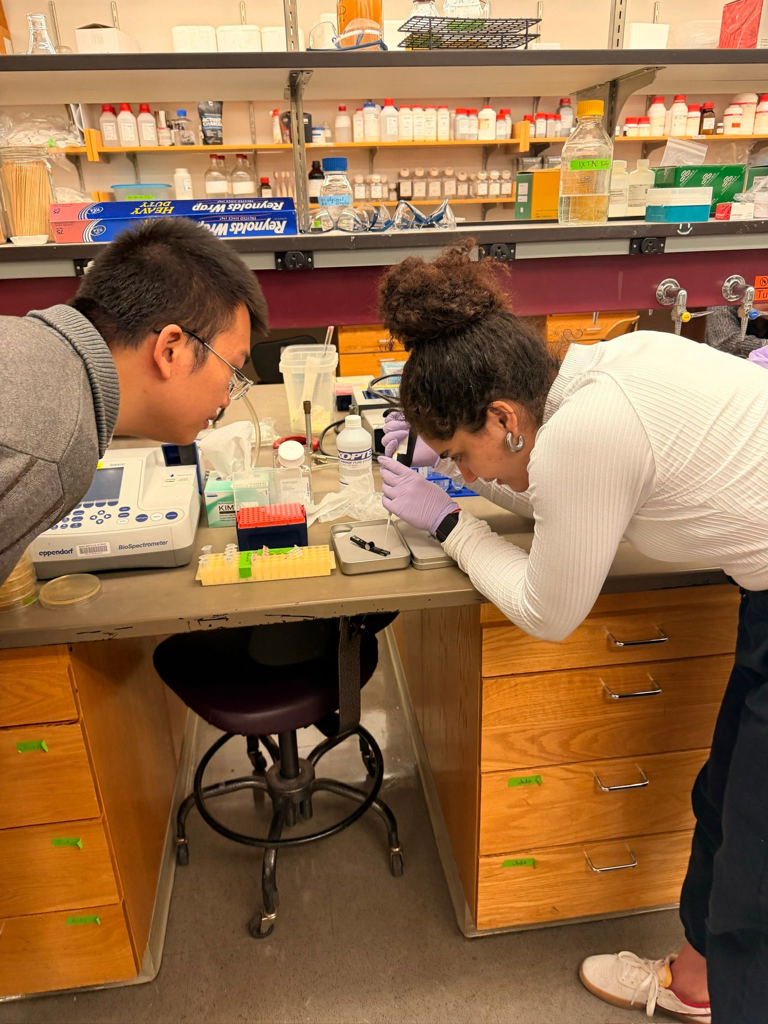
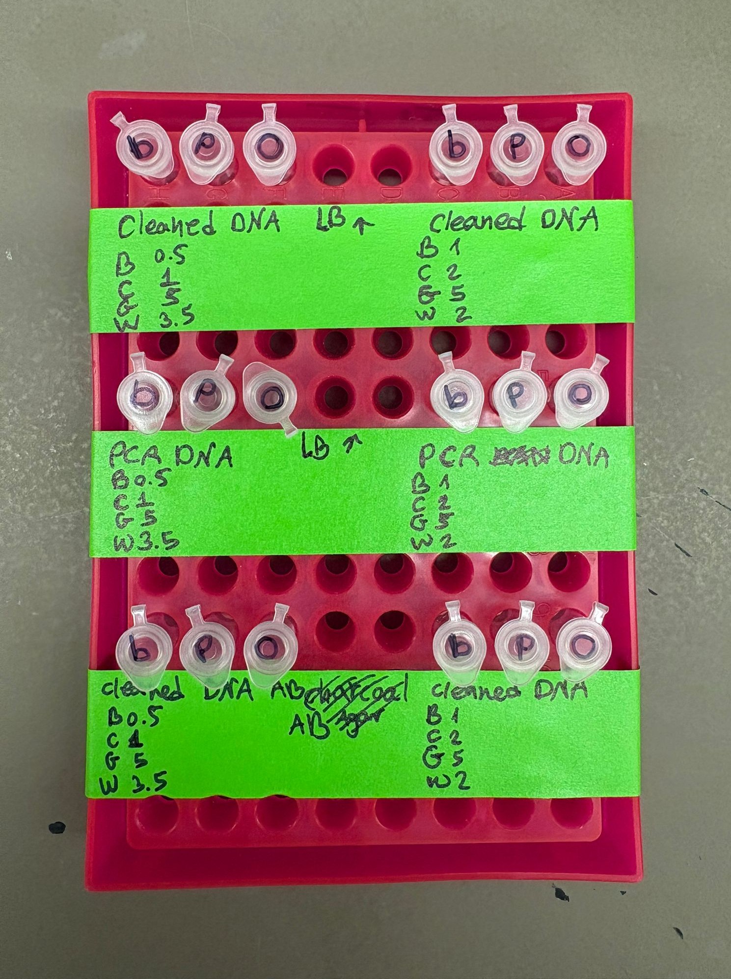
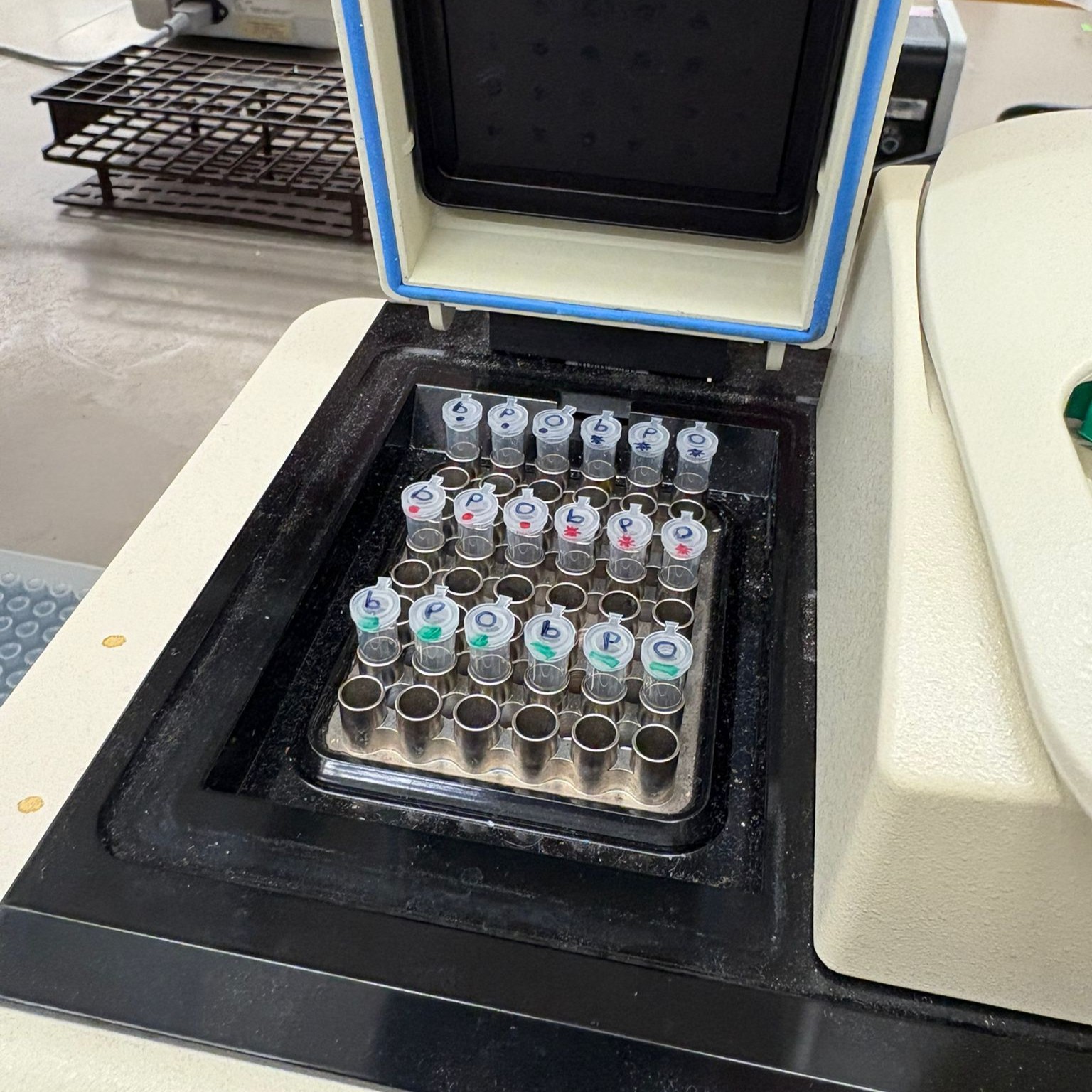
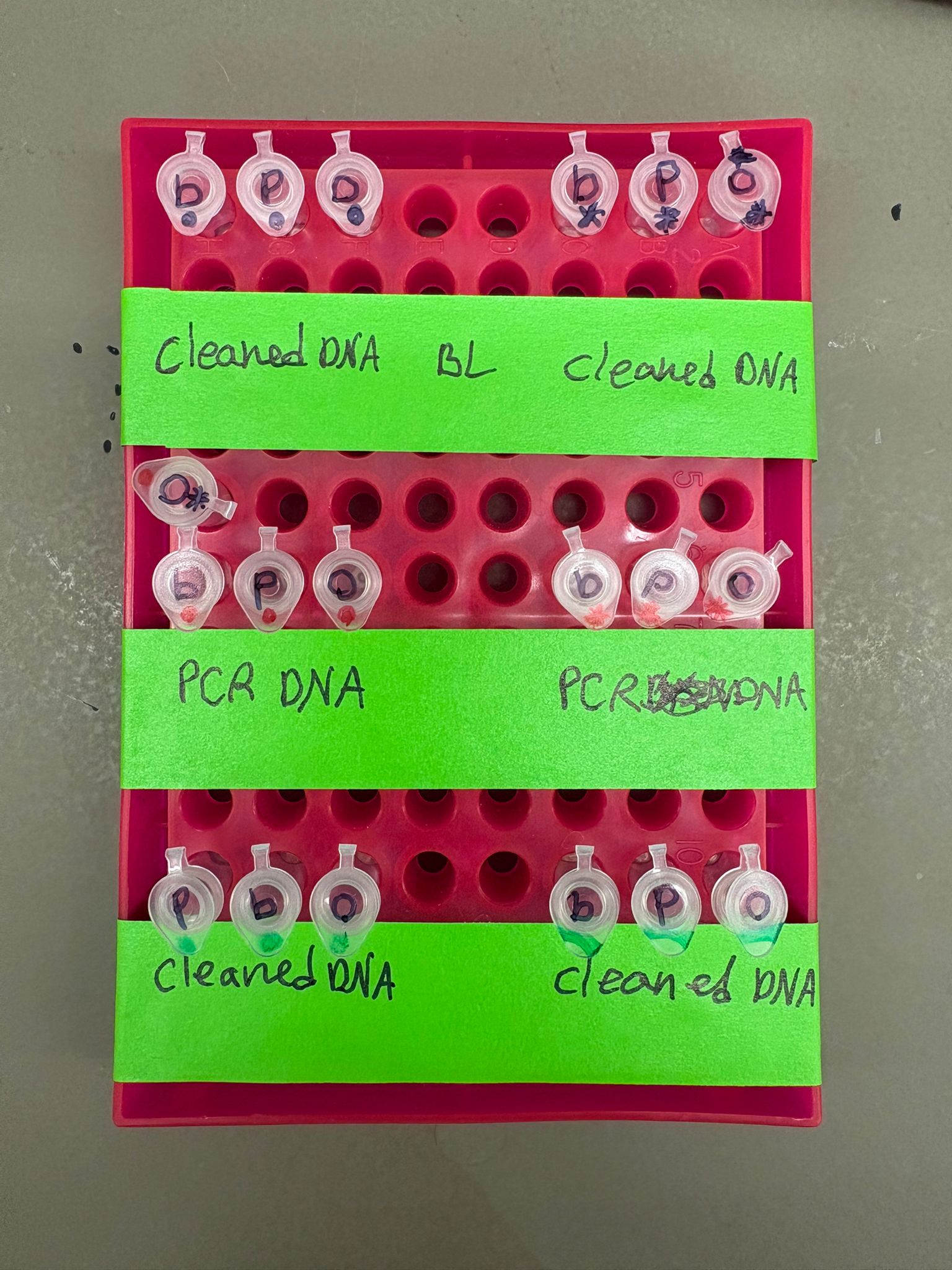
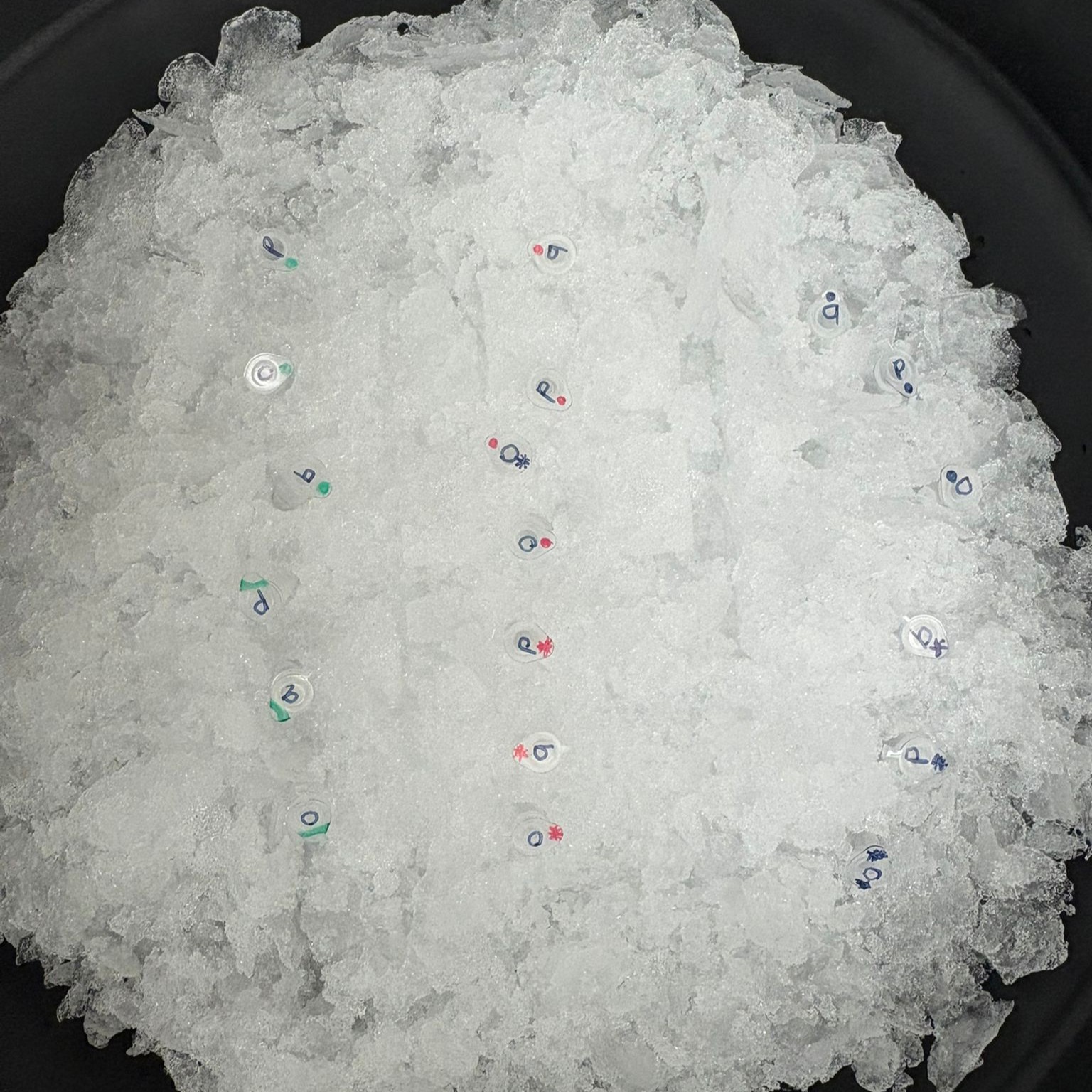
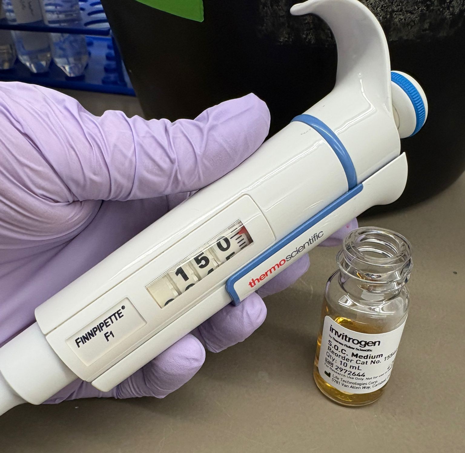
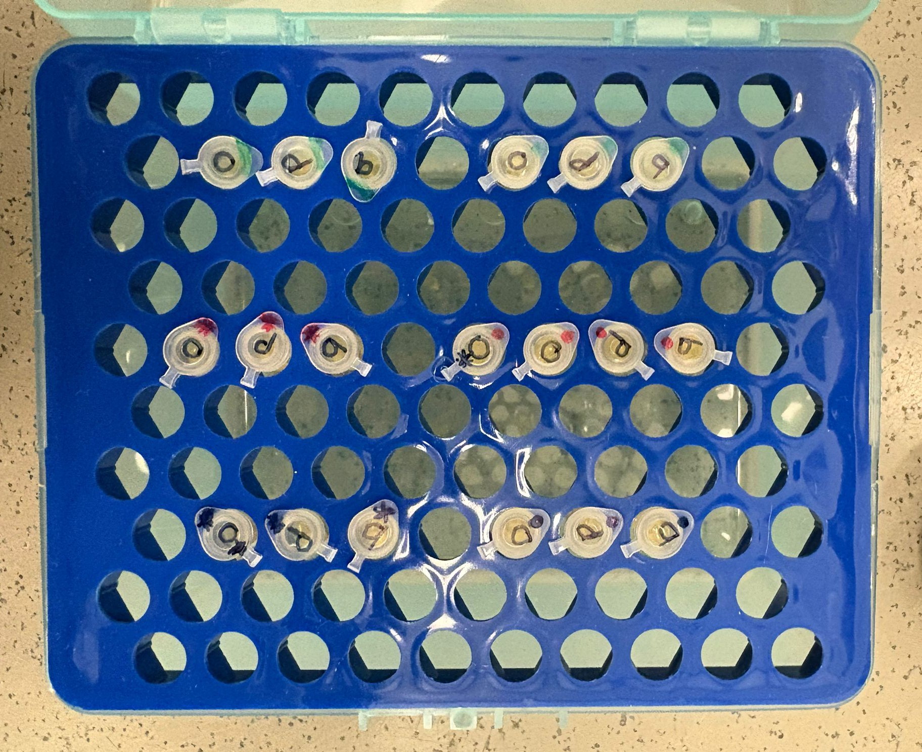
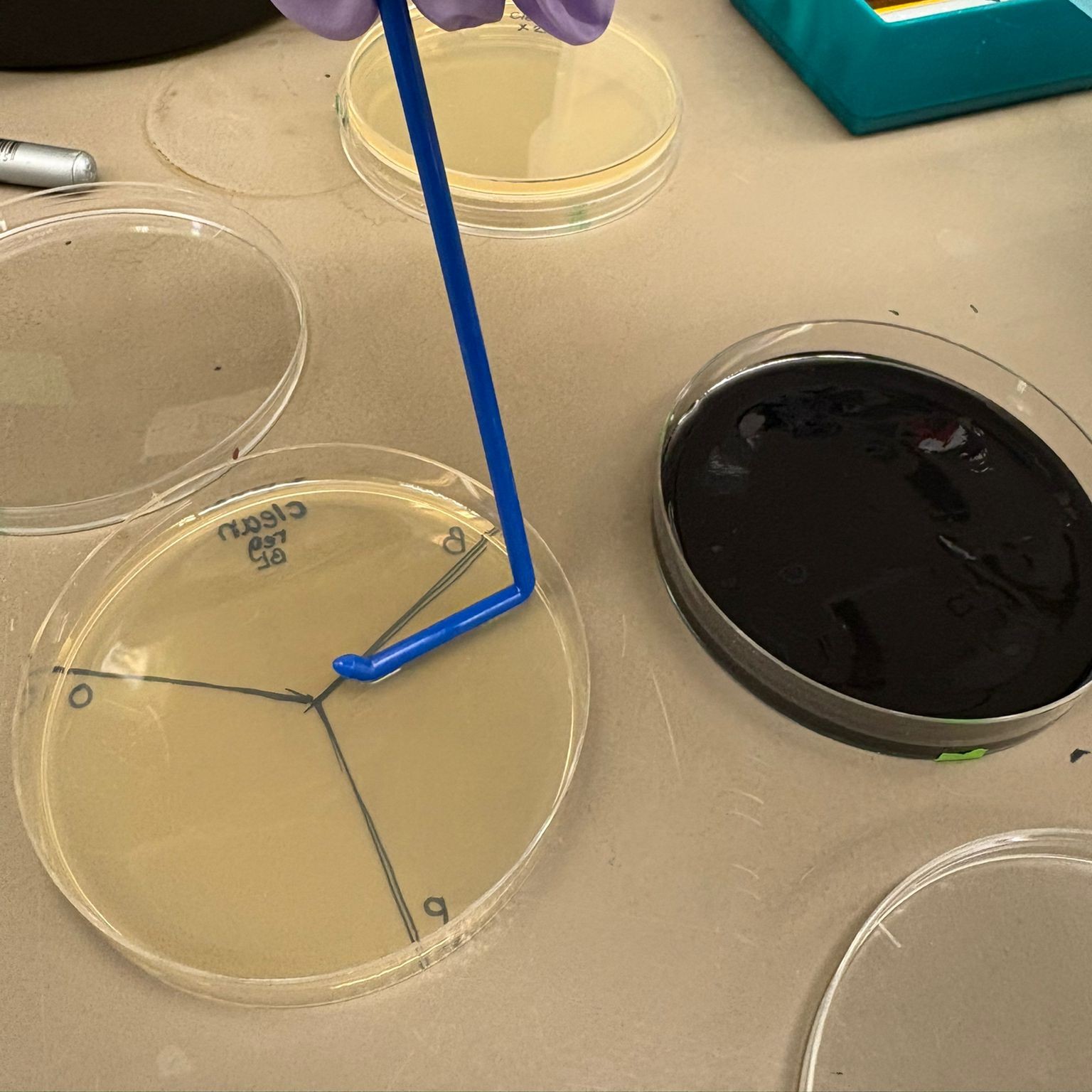
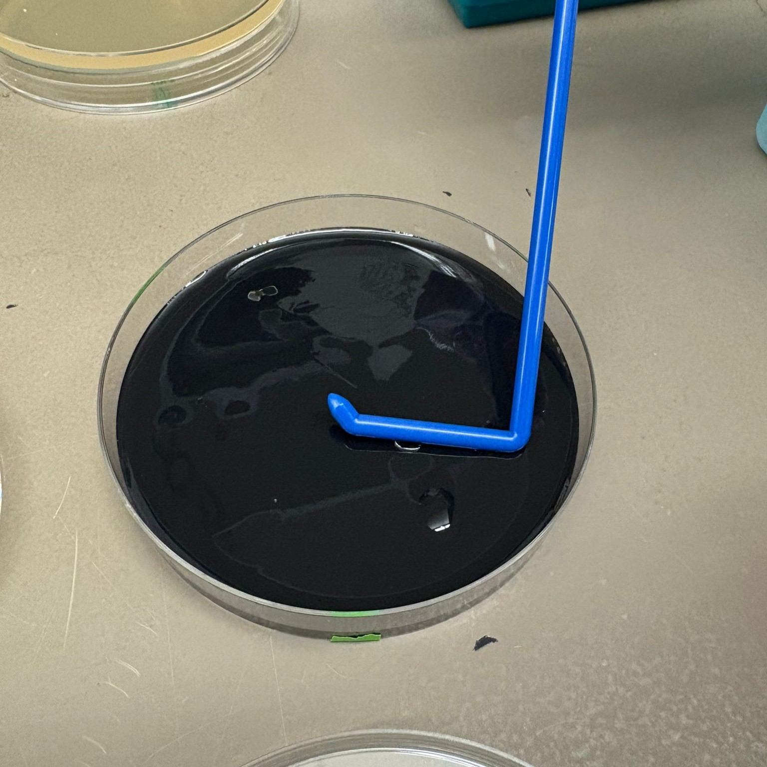
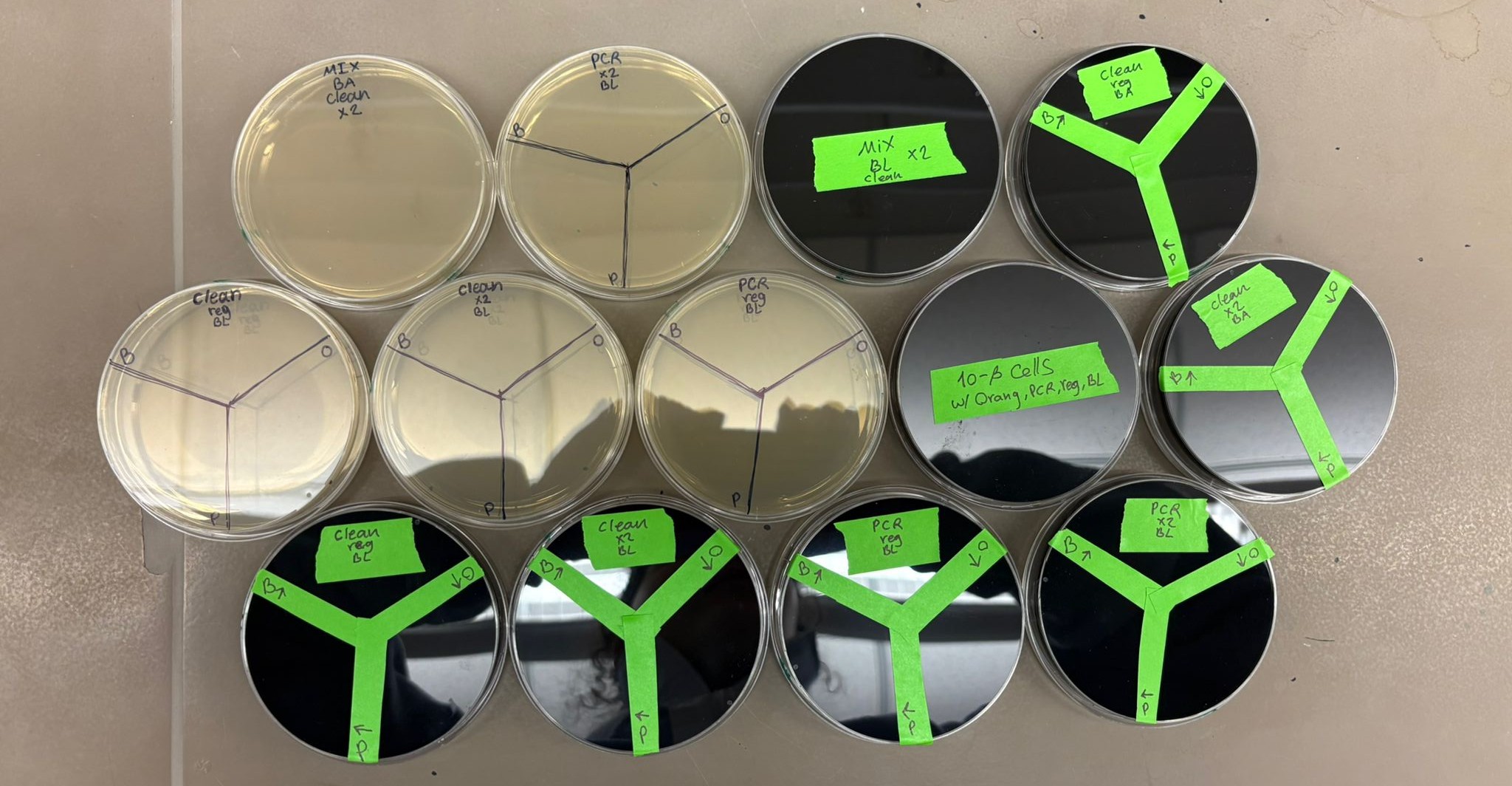
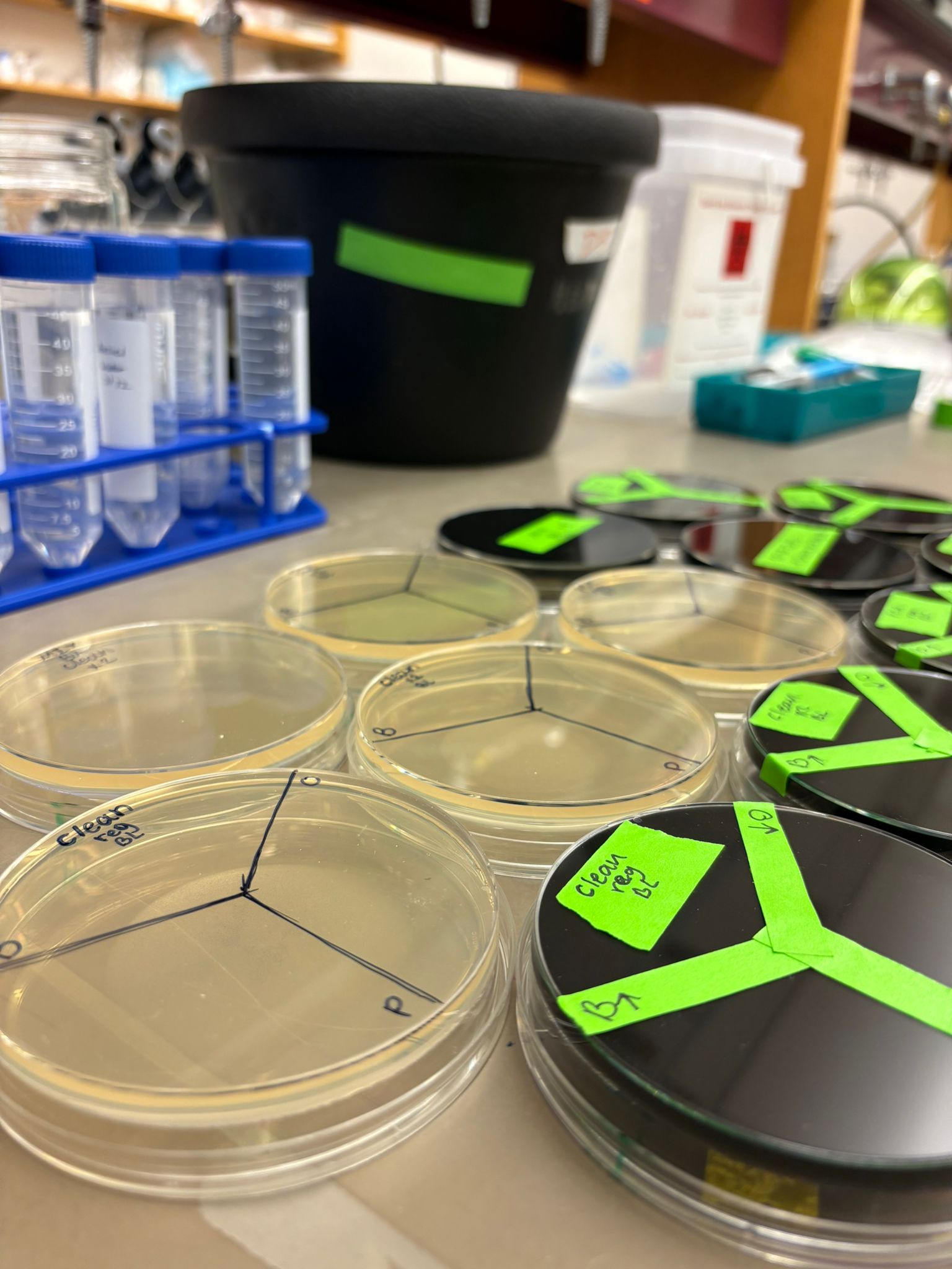
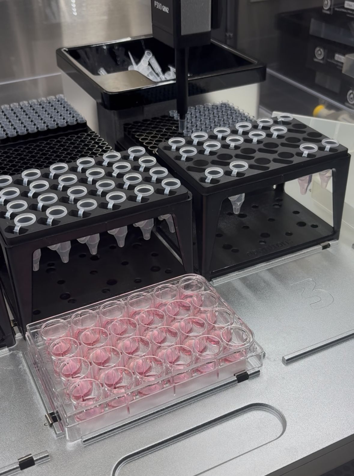
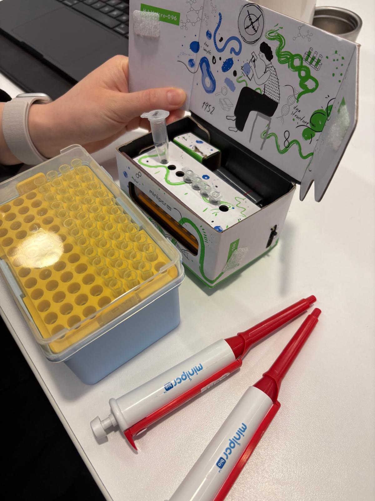
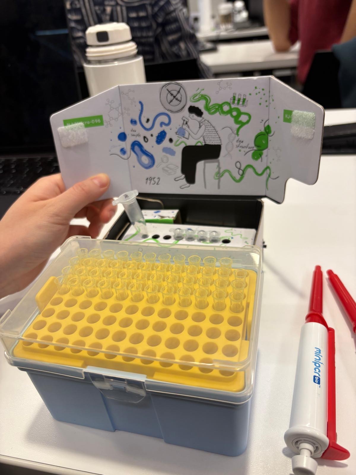
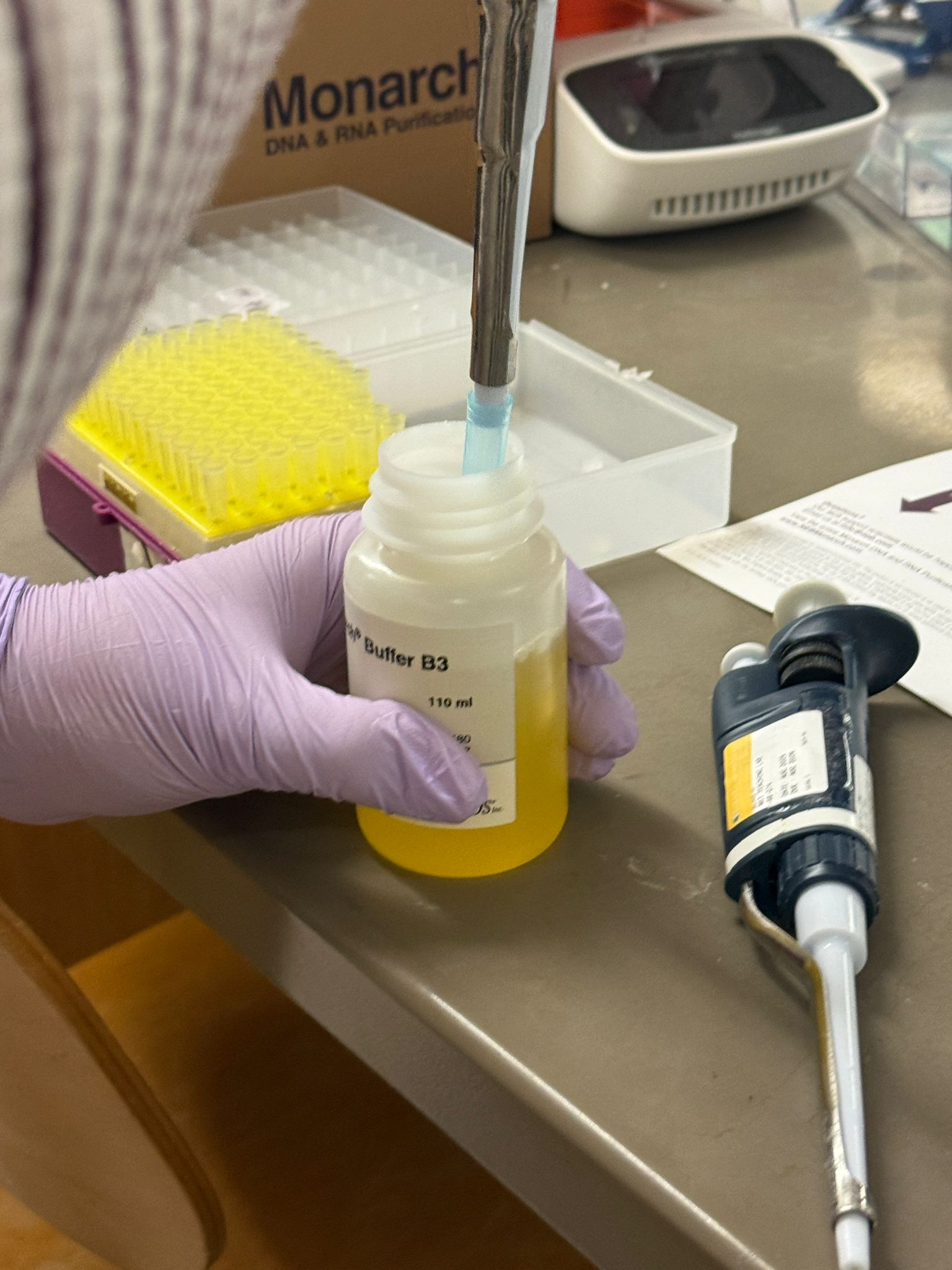
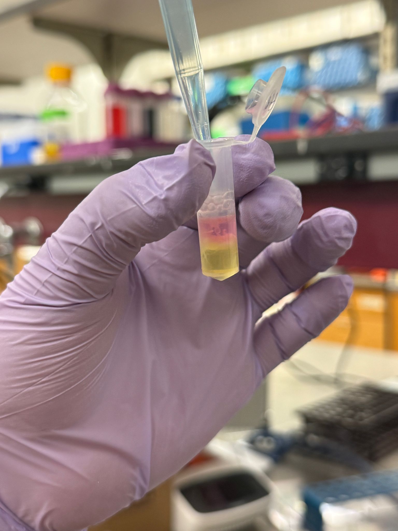
In the lab, we uploaded the design protocol to the Opentrons, loaded the trays with the engineered E. coli, the black (charcoal) agar plate, pipette tips, and a “trash” bin. It was fascinating to watch the machine work. I was especially happy to discover that the Opentrons OT-2 operates using a 3D gantry system - very similar to 3D printers and CNC cutters - which made it very intuitive for me to use (and fun to watch).

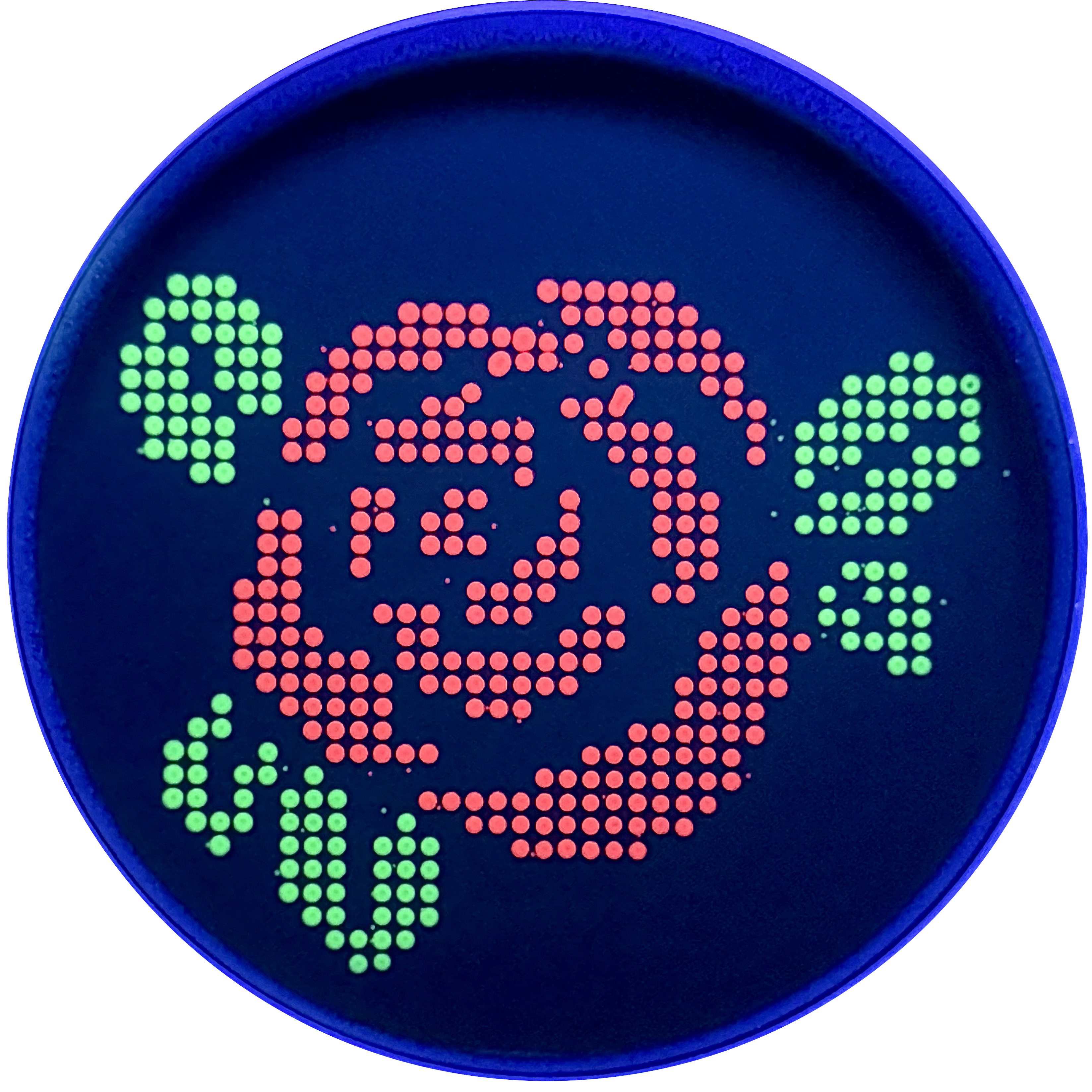
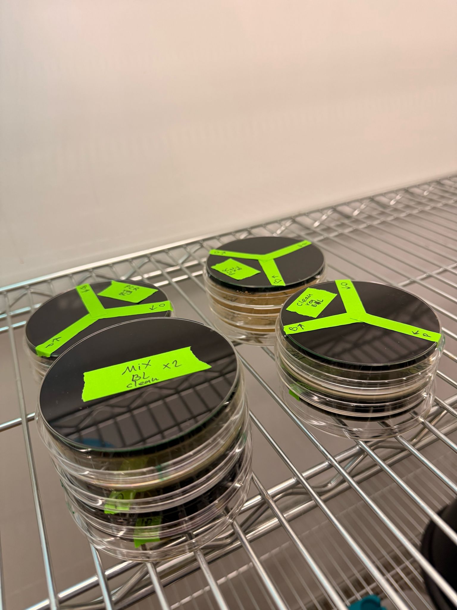
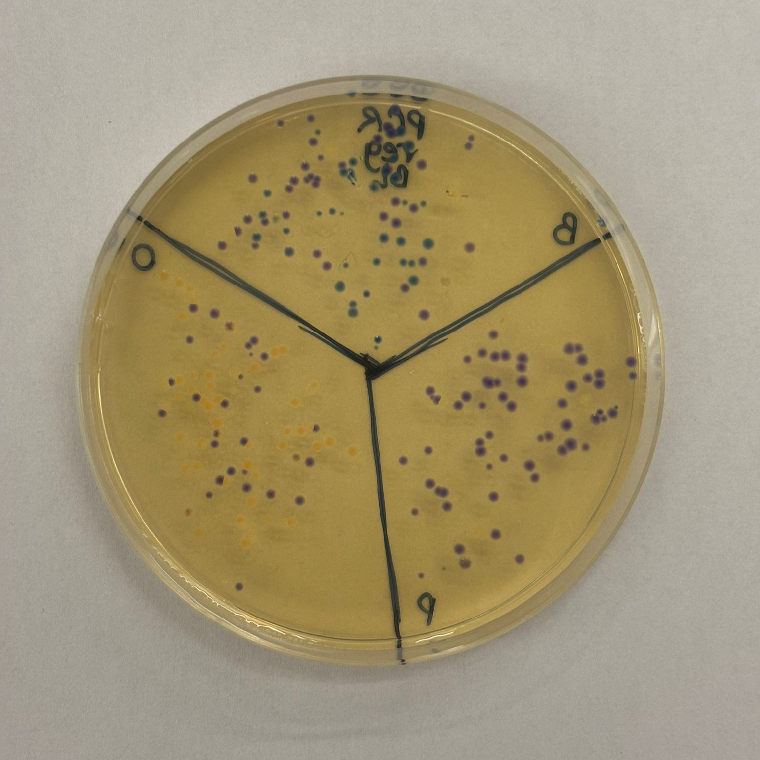
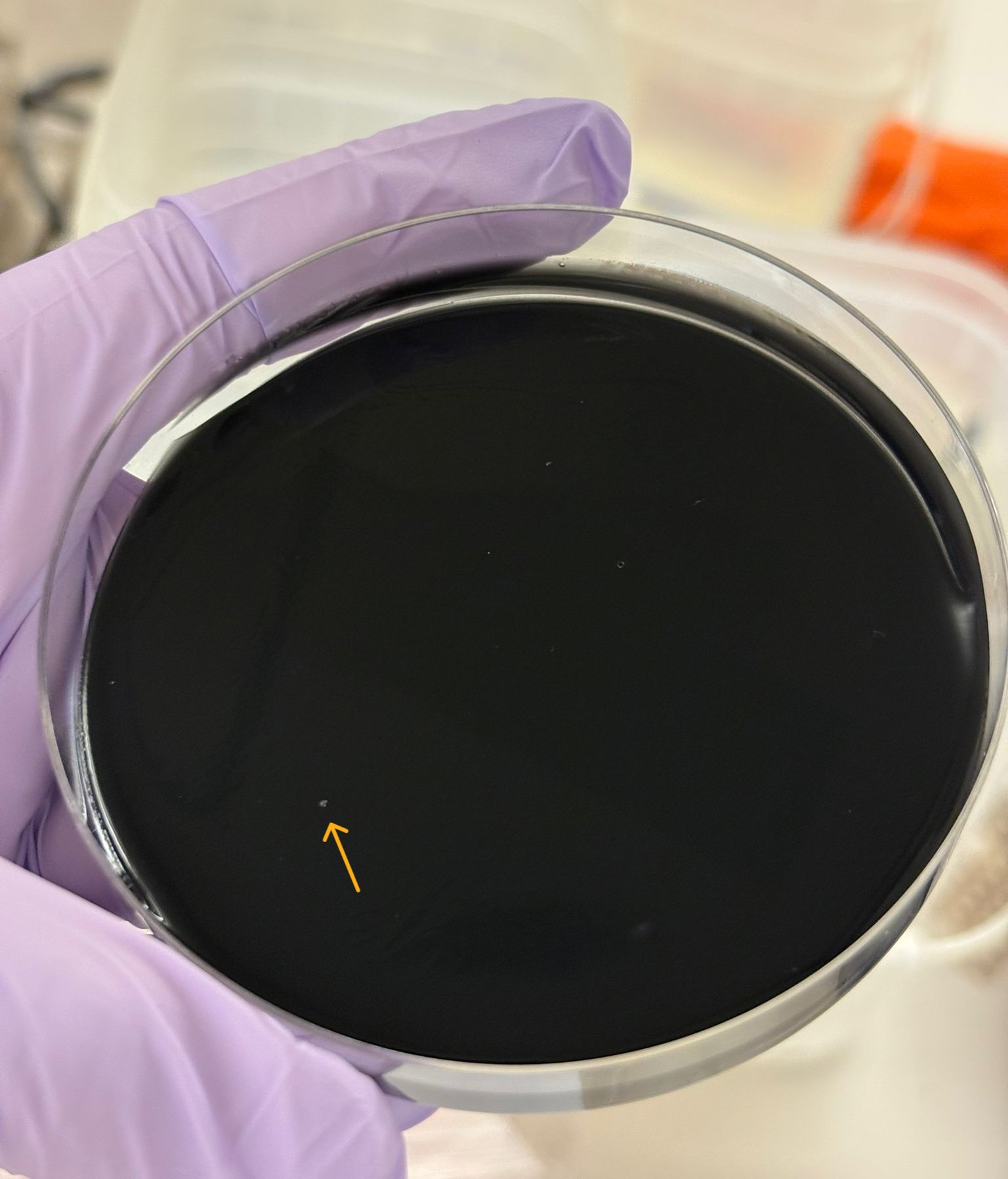
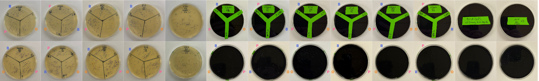
After “the print” was finished, we placed the agar plates in the incubator overnight and photographed them under UV light the following day.

The results were AMAZING!

My Earth design:

My Cross-Stitch Rose design:

All of the amazing designs students have made:

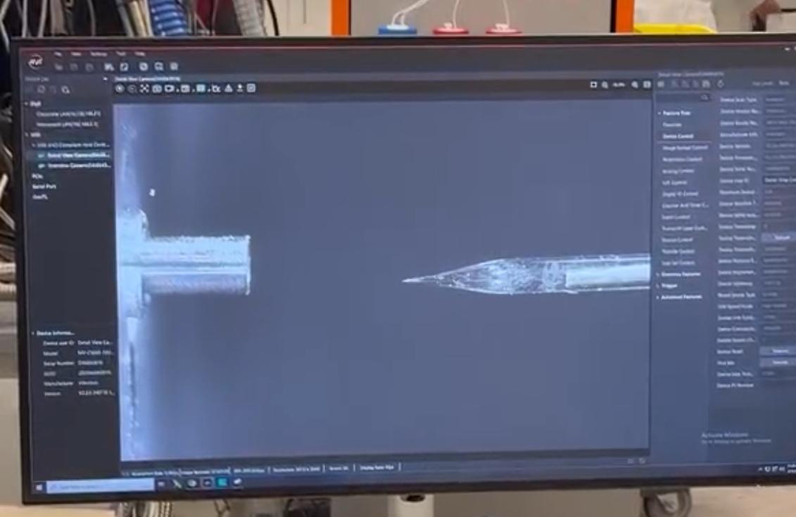
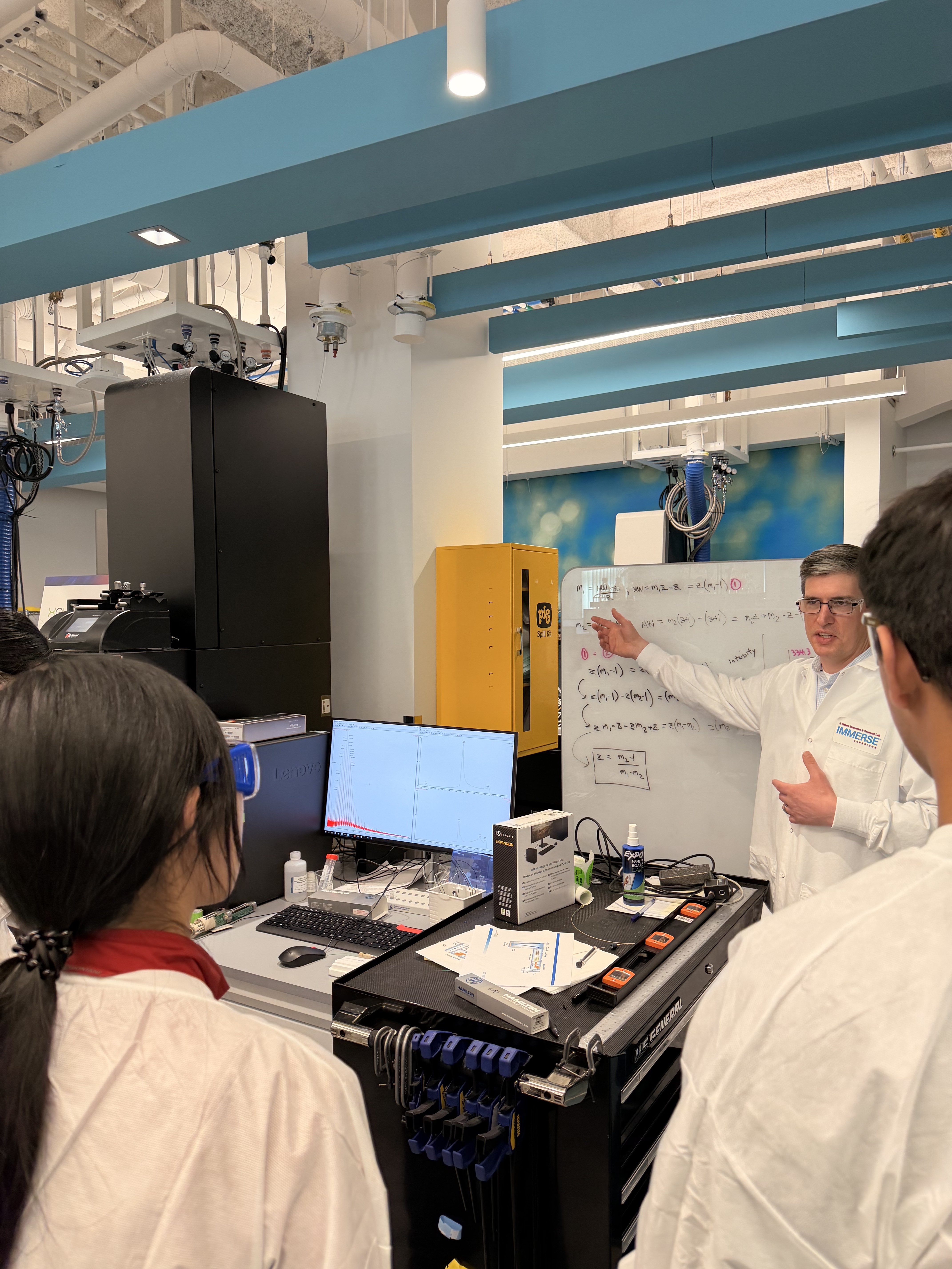
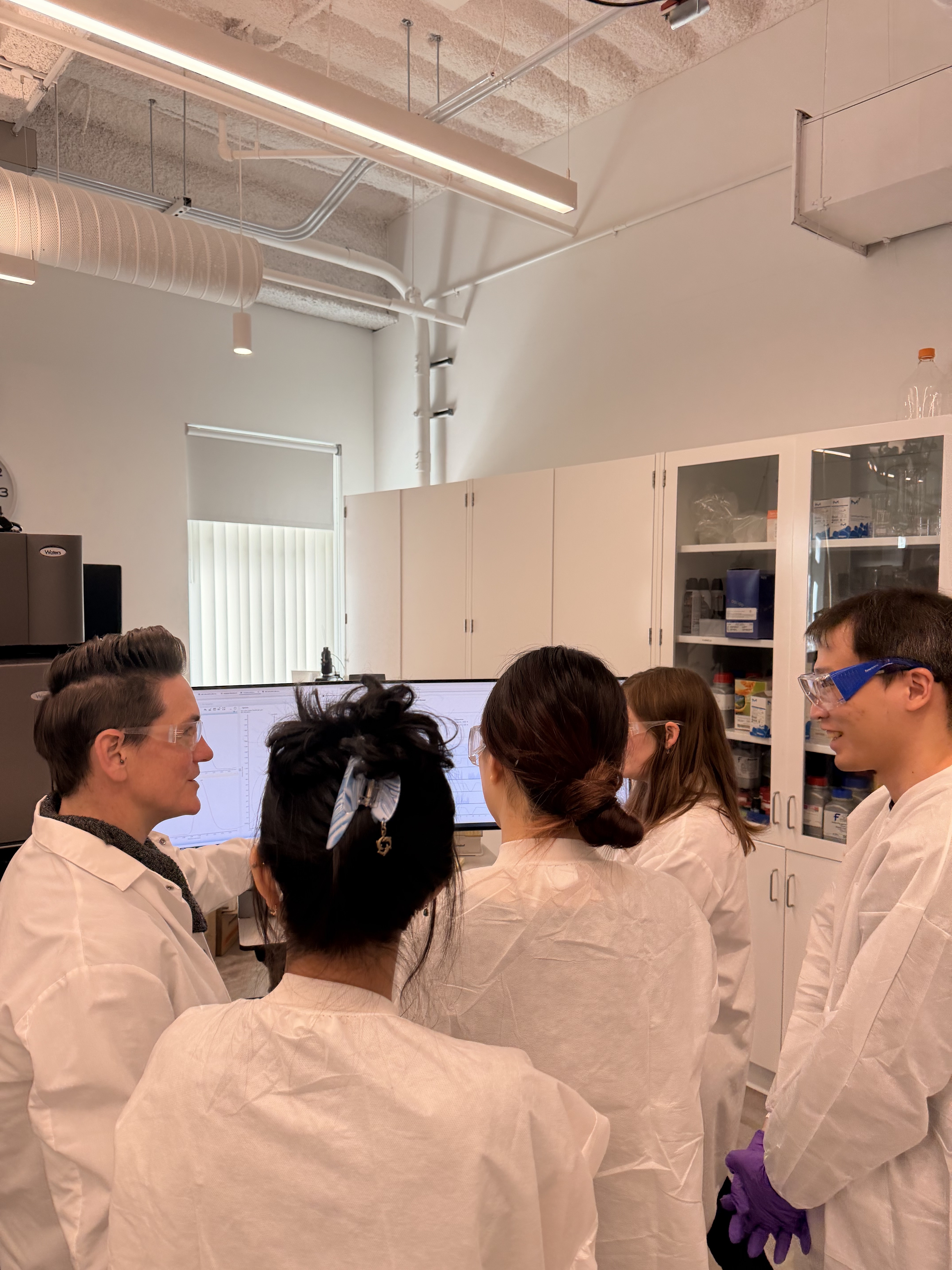
On Saturday, I had the honor of visiting the Ginkgo Bioworks labs in Boston, where I saw how the Nebula (the RAC system at Ginkgo Bioworks) works, and even loaded another design of mine onto it. This time, I used a rectangular composition and painted the Israeli Sabra cactus - or in modern Hebrew, Tzabar - which reminds me of sweet childhood memories and my lovely country.

Here it is - My Tzabar Cactus design:

This definitely won’t be my last experiment with bio art - I’m already looking forward to bringing lab automation into my final project.

*Also, this cool idea reminded me of a game I used to play whenever I was bored. I won’t tell you anything about it —-except that it involves koalas. Here is the link to the game

Week 6 Lab: Lab Gibson Assembly

In this week’s 2-day lab, we learned how to construct a plasmid using Gibson assembly and genetically engineer E. coli. Our goal was to mutate the chromophore of amilCP, a purple chromoprotein originally from the coral Acropora millepora, to generate new color variants. Using PCR with mutation-introducing primers, we modified the gene and assembled it into a plasmid containing the elements needed for replication and expression in bacteria. The plasmid was then transformed into E. coli so the cells could produce the engineered protein.

I had the pleasure of working with Asaf, and it was especially exciting to apply techniques I had heard about for years in class - PCR, plasmid assembly, and bacterial transformation - and actually perform them myself in the lab. Watching these abstract molecular biology concepts turn into real experiments (and eventually colorful bacteria) made the whole process feel much more tangible. So come join us on this cloning adventure!

We mainly followed the lab protocol that can be found in this week’s lab page on the HTGAA 2026 website. If a change was made, it will be noted here.

PCR and DNA Purification

Polymerase Chain Reaction (PCR)

The first step of the experiment was to amplify fragments of the plasmid containing the amilCP gene and introduce mutations using PCR. We started with a plasmid that already contained the gene along with the necessary elements for replication and expression. Using different forward primers, we introduced mutations in the chromophore region of the gene while amplifying the DNA. The PCR reactions were designed so that the plasmid was effectively split into two linear fragments: one corresponding to the plasmid backbone and the other containing the mutated gene.

We chose to try and create the orange, blue, and light pink mutations of the gene. Each of us prepared our own PCR mixtures — I prepared one backbone reaction along with the three color variants, while Asaf prepared four backbone reactions.

After preparing the reactions, the tubes were briefly centrifuged and placed in the thermocycler, which carried out repeated cycles of denaturation, primer annealing, and extension to amplify the desired DNA fragments.

The full compositions and concentrations for each PCR reaction are summarized in the tables below.

DpnI Digest

Placeholder — I will add details here once I confirm whether this step was performed.

DNA Purification and Quantification

Gel Electrophoresis

After the PCR was completed, we selected the three color variants, the backbone reaction I prepared (which we refer to as BL from now on), and one of Asaf’s backbone reactions that he arbitrarily chose from his set (which we refer to as BA) and ran them on a gel to check whether the PCR worked as expected.

We first vortexed the PCR reactions and then prepared the samples for loading according to the following table:

We then ran the gel electrophoresis and obtained the following result:

As seen in the gel, we obtained the expected fragments for the orange and blue variants, as well as for both backbone reactions (BL and BA). However, we did not observe a band in the light pink lane, suggesting that something likely went wrong during that PCR reaction. Despite this, we continued to carry the light pink sample through the rest of the protocol.

DNA Purification and Quantification

After verifying the PCR products on the gel, we proceeded with DNA cleanup using a spin-column purification kit. For each sample, we added DNA binding buffer at a 5:1 ratio relative to the PCR product volume and mixed the solution by vortexing.

The mixtures were then transferred to Zymo spin columns placed in collection tubes and centrifuged to allow the DNA to bind to the column matrix.

We then performed the wash step using DNA wash buffer, centrifuging after each wash and repeating this step twice to ensure proper purification of the DNA.

Finally, the DNA was eluted from the column using elution buffer, resulting in purified PCR products ready for downstream applications.

Here are the results we had at the end of the first day of this lab:

The image shows the PCR products for the three color variants and five backbone reactions, the diluted PCR products for the three colors along with BA and BL, and the cleaned PCR products for all reactions. In the labeling, BA is marked as “B” with a green dot, while BL is marked as “B” with a purple dot.

At the end of the day, we stored the purified DNA samples in the fridge and continued the experiment the following day.

Concentration Measurement – Nanodrop

We started the second day by using a NanoDrop spectrophotometer to measure the DNA concentration of our cleaned samples. For each measurement, we loaded 2 µL of sample onto the machine.

We first measured one of the cleaned backup backbone samples and obtained the following result:

As shown, the concentration was 8.7 µg/mL, which is significantly lower than the values we expected (around ~20 µg/mL).

We then measured another cleaned backbone sample, this time BL, which gave a slightly better result of 12.5 µg/mL, but still lower than desired.

At this point, we decided to measure the concentration directly from the original PCR products (without cleanup). We first tested the BA PCR sample and obtained a much higher reading of 449.5 µg/mL:

We then measured the BL PCR sample, which showed a concentration of 486.2 µg/mL:

These values are likely overestimates of the true DNA concentration due to the presence of primers, nucleotides, and other components in the PCR mixture. However, they were clearly much higher than the cleaned samples, suggesting that the cleanup step may have resulted in significant DNA loss.

Gibson Assembly

For this part, we used Gibson Assembly to recombine the PCR-generated fragments into complete plasmids. We designed 6 different assemblies for each color variant (18 total), varying three main parameters:

• DNA source: cleaned vs. uncleaned PCR product (referred to as PCR)
• Backbone type: BL for PCR samples, and both BL and BA for cleaned samples
• Assembly composition: either according to the standard protocol or a modified version (x2) to compensate for the low DNA concentrations observed after cleanup

The standard assembly mixture (based on the protocol) was:

To account for the low concentrations observed after cleanup, we designed a modified version (x2):

All assembly combinations are summarized in the table below:

Legend:
💙 = Blue 🩷 = Light Pink 🧡 = Orange

We then prepared the different assembly reactions by pipetting the required components into labeled tubes.

After preparing the mixtures, the tubes were incubated to allow the fragments to assemble into complete plasmids.

Finally, the assembled plasmids were ready for transformation into E. coli.

Transformation

For this part, we transformed the assembled plasmids into competent E. coli cells. We added the Gibson assembly products to chemically competent cells and incubated the mixtures on ice for 30 minutes to allow the DNA to associate with the cells.

After heat shock (following the protocol), we added SOC medium to allow the cells to recover. While the protocol suggests 200–500 µL, we used 150 µL of SOC for each sample per Ronan’s reccomendation.

The tubes were then placed in a shaking incubator to promote recovery and expression of the antibiotic resistance gene.

We used standard DH5α competent cells for most transformations. However, for the orange, cleaned BL, x2 assembly, we also used 10-beta competent cells to boost transformation efficiency. In addition, we performed a separate transformation of the orange PCR BL (standard concentration) using only 10-beta cells. In total, we performed 19 transformations.

After the 60 minute growth period in the shaking incubator, we proceeded with plating the transformed cells onto agar plates.

For the cleaned BL and PCR BL assemblies (both concentrations), we divided standard agar plates into thirds and plated a different color variant in each section. We also prepared a plate containing a mixture of all three colors from the BA cleaned DNA x2 assembly (we called it MIX).

We then used charcoal agar plates from the Opentrons art lab to create additional plates, since we observed some background growth on the regular plates from a control that was done earlier (colonies that likely did not take up the plasmid). We therefore wanted to use plates that we knew provide more reliable selection, and also explore the improved visual contrast offered by the charcoal medium.

For each assembly type, we again divided the plates into thirds and plated a different color in each section, this time for all assemblies. In addition, we prepared:

• A mixed plate of all three colors from the BL cleaned DNA x2 assembly
• A plate containing only the orange PCR BL (10-beta only) transformation

For plates containing all three colors, we plated 40 µL of each sample. For plates containing a single sample, we plated 100 µL.

Finally, the plates were incubated for approximately 36 hours to allow colony growth.

Results

After 36 hours, the plates were taken out of the incubator and stored in the fridge.

Overall, we successfully completed the experiment. The mutation that performed best across the different assemblies was blue, followed by orange (with slightly less consistent success across plates). As expected from the gel results, the light pink variant did not appear in any of the plates, except for one potential colony on the MIX BL clean x2 plate. However, it is unlikely to be truly pink, since no corresponding signal was observed elsewhere.

The best overall result was obtained from the PCR, regular concentration, BL assembly, which produced many clear blue and orange colonies:

This result suggests that the uncleaned PCR samples actually performed better in the assembly, likely because they retained a much higher DNA concentration, while the cleanup step may have reduced the available DNA more than expected.

We observed slightly fewer colonies on the charcoal plates. This may suggest stronger selection conditions or differences in growth on the charcoal medium. However, these plates still provided useful results and allowed us to observe the colony colors against a dark background (although the contrast was somewhat less distinct than expected). Here as well, the best-performing condition was PCR, regular concentration, BL:

The special transformation using 10-beta competent cells for the orange variant was not successful overall, with only a single colony observed on the charcoal plate:

Here are the results we obtained across all plates:

Overall, this was a great experience. Seeing E. coli colonies appear in different colors was especially exciting, and it was very fun to apply techniques we had previously only learned about in theory. I’m really glad I had the opportunity to carry out this full workflow in practice.

See you next time! :)

Week 7 Lab: Lab Neuromorphic Circuits and Biomaterials

In this week’s lab, we designed neuromorphic genetic circuits (IANNs) using the Neuromorphic Wizard and learned how intracellular systems can perform analog computations and approximate universal functions. The Opentrons OT-2 then created our designs and transfected them into HEK293 cells in the Weiss Lab. In addition, we worked with mycelium by packing it into molds to grow everyday objects!

Neuromorphic Genetic Circuits (IANNs)

Initially, I wanted to design a function that would create a diamond shape, but I realized that it was much more difficult than expected to define it mathematically in the first quadrant, and even harder to implement using the Neuromorphic Wizard. I therefore decided to recreate one of the designs presented in lecture by Prof. Ron Weiss, the Dual Region TRBL (Top Right Bottom Left) circuit, in order to better understand the key concepts.

Here is my final design as a diagram:

Here is the .csv file I inputted to the wizard:

Here is the prediction of the wizard for the behavior of the circuit:

The following day, I observed the Opentrons building the circuit and using lipid nanoparticles to insert it into HEK293 cells in the lab:

Here is the actual data from the constructed circuit in the HEK293 cells:

As you can see, the results turned out as expected. It was interesting to observe the effect of the different bias concentrations, and it made me wonder how the behavior would change if one of the inputs (X₁ or X₂) was removed.

Mycelium-Based Biomaterials

For this part of the lab, I first brainstormed ideas for what I wanted to make. Initially, I thought about creating something larger, like a chair or a table, but due to the limited amount of material available, I decided to make a small lampshade:)

I explored different shapes and decided on a design inspired by a mushroom. I used Fusion 360 to first create the positive shape of the lampshade:

Then, I created the negative mold from that design:

Next, mold was printed using the P2S Bambu Lab printer:

In the lab, I mixed the growth medium and packed it into the mold:

The mold was then left to sit and grow:

The results will be ready in a few weeks!