Week 6 Lab: Lab Gibson Assembly
In this week’s 2-day lab, we learned how to construct a plasmid using Gibson assembly and genetically engineer E. coli. Our goal was to mutate the chromophore of amilCP, a purple chromoprotein originally from the coral Acropora millepora, to generate new color variants. Using PCR with mutation-introducing primers, we modified the gene and assembled it into a plasmid containing the elements needed for replication and expression in bacteria. The plasmid was then transformed into E. coli so the cells could produce the engineered protein.
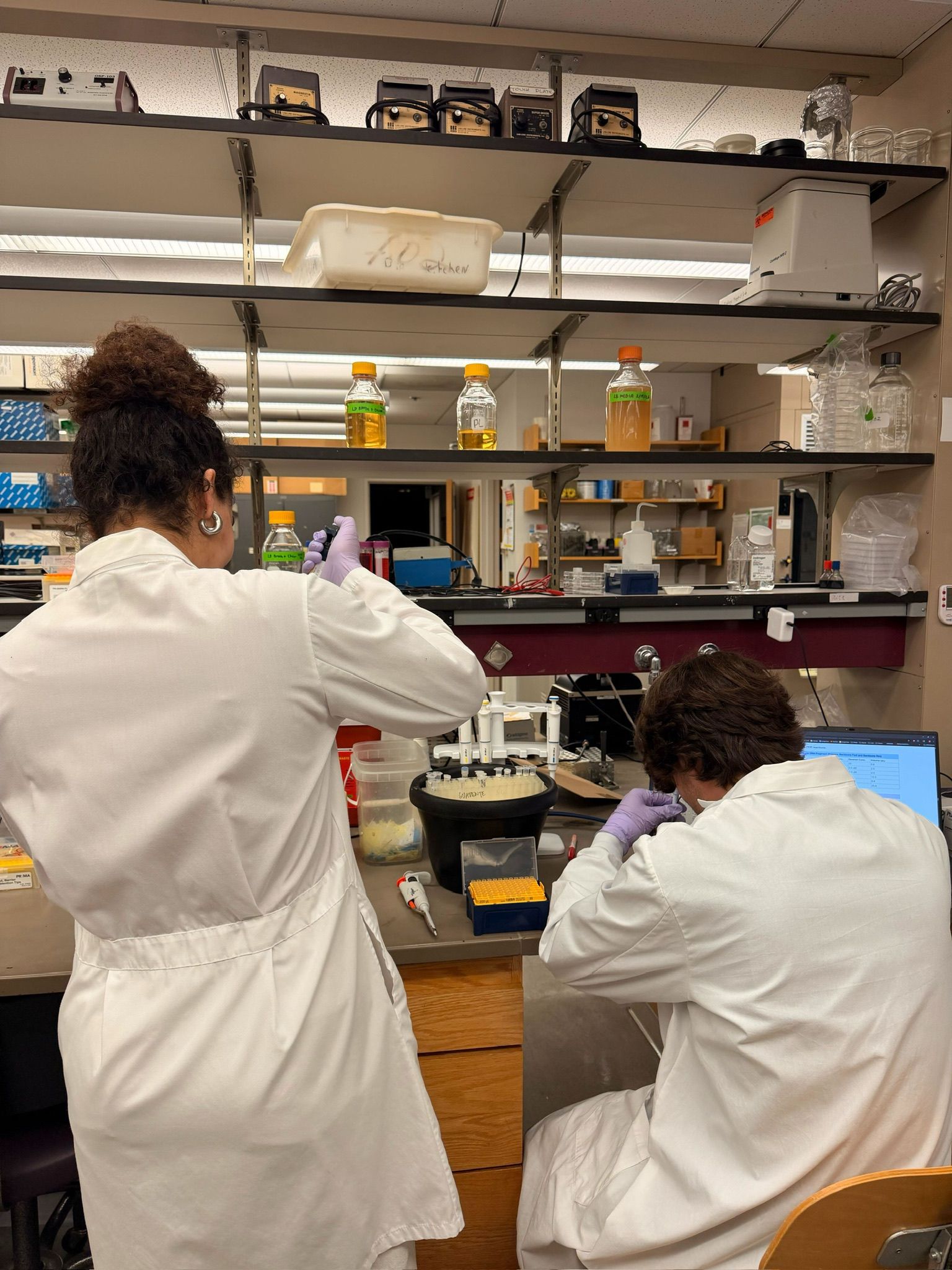
I had the pleasure of working with Asaf, and it was especially exciting to apply techniques I had heard about for years in class - PCR, plasmid assembly, and bacterial transformation - and actually perform them myself in the lab. Watching these abstract molecular biology concepts turn into real experiments (and eventually colorful bacteria) made the whole process feel much more tangible. So come join us on this cloning adventure!
We mainly followed the lab protocol that can be found in this week’s lab page on the HTGAA 2026 website. If a change was made, it will be noted here.
PCR and DNA Purification
Polymerase Chain Reaction (PCR)
The first step of the experiment was to amplify fragments of the plasmid containing the amilCP gene and introduce mutations using PCR. We started with a plasmid that already contained the gene along with the necessary elements for replication and expression. Using different forward primers, we introduced mutations in the chromophore region of the gene while amplifying the DNA. The PCR reactions were designed so that the plasmid was effectively split into two linear fragments: one corresponding to the plasmid backbone and the other containing the mutated gene.
We chose to try and create the orange, blue, and light pink mutations of the gene. Each of us prepared our own PCR mixtures — I prepared one backbone reaction along with the three color variants, while Asaf prepared four backbone reactions.
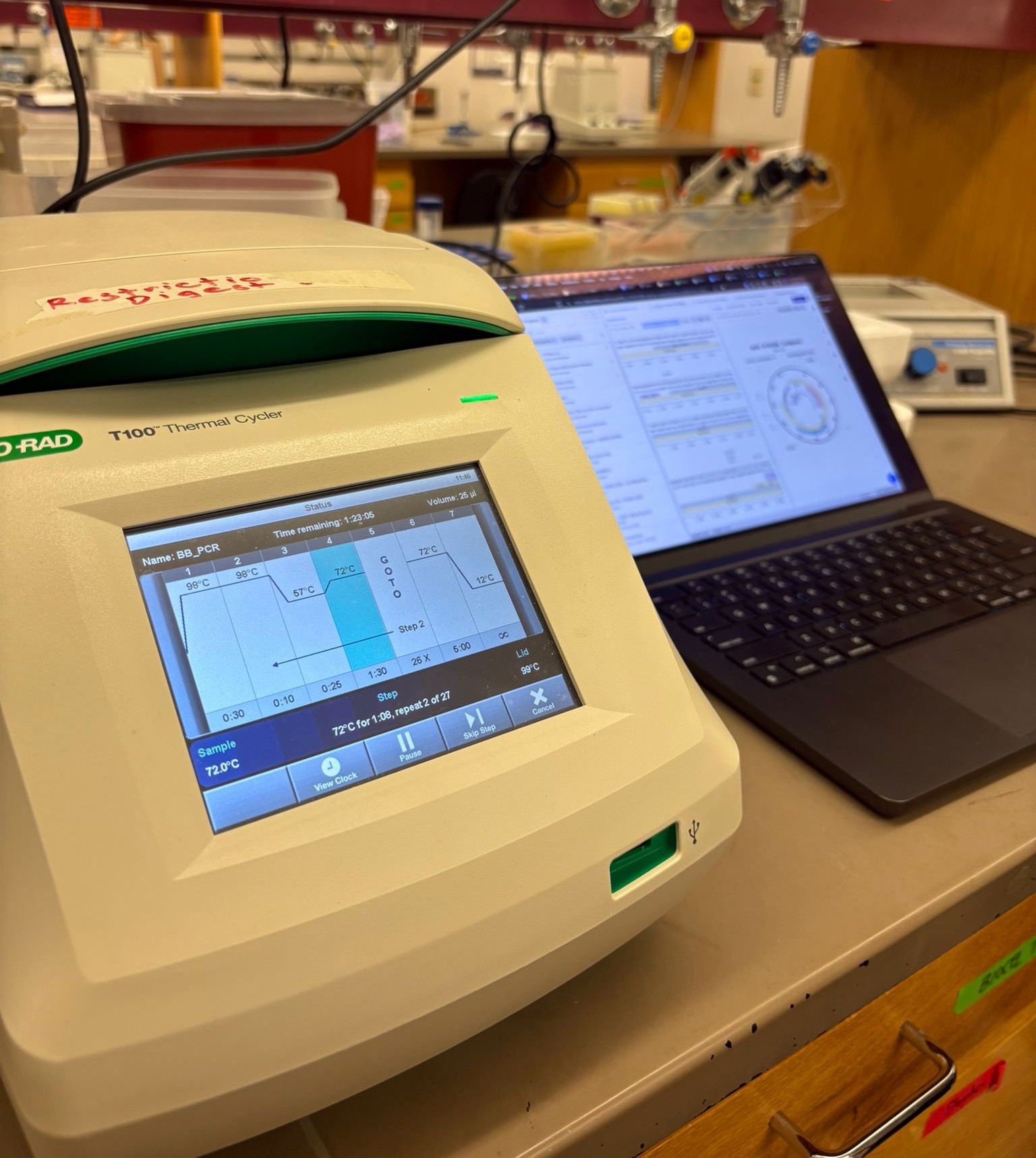
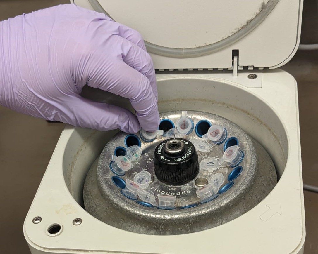
After preparing the reactions, the tubes were briefly centrifuged and placed in the thermocycler, which carried out repeated cycles of denaturation, primer annealing, and extension to amplify the desired DNA fragments.
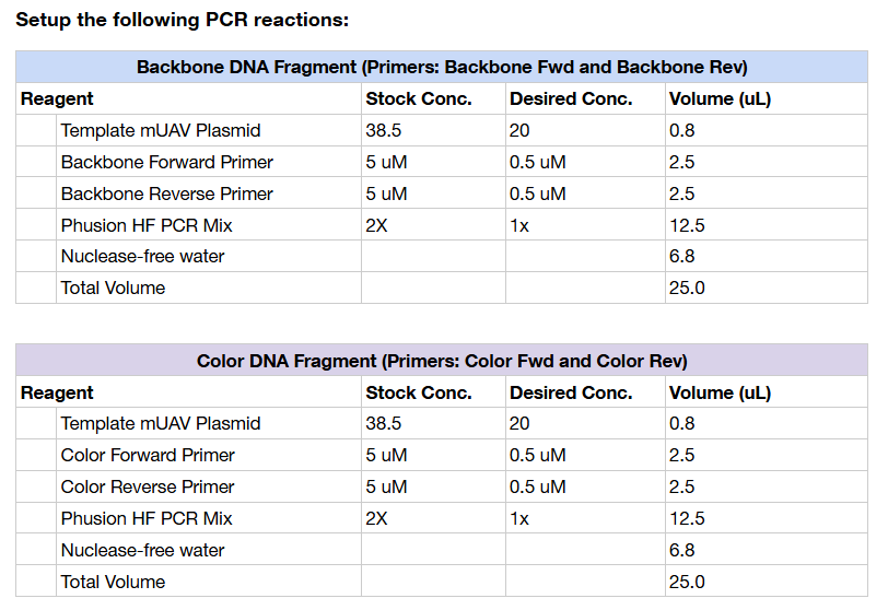
The full compositions and concentrations for each PCR reaction are summarized in the tables below.
DpnI Digest
Placeholder — I will add details here once I confirm whether this step was performed.
DNA Purification and Quantification
Gel Electrophoresis
After the PCR was completed, we selected the three color variants, the backbone reaction I prepared (which we refer to as BL from now on), and one of Asaf’s backbone reactions that he arbitrarily chose from his set (which we refer to as BA) and ran them on a gel to check whether the PCR worked as expected.
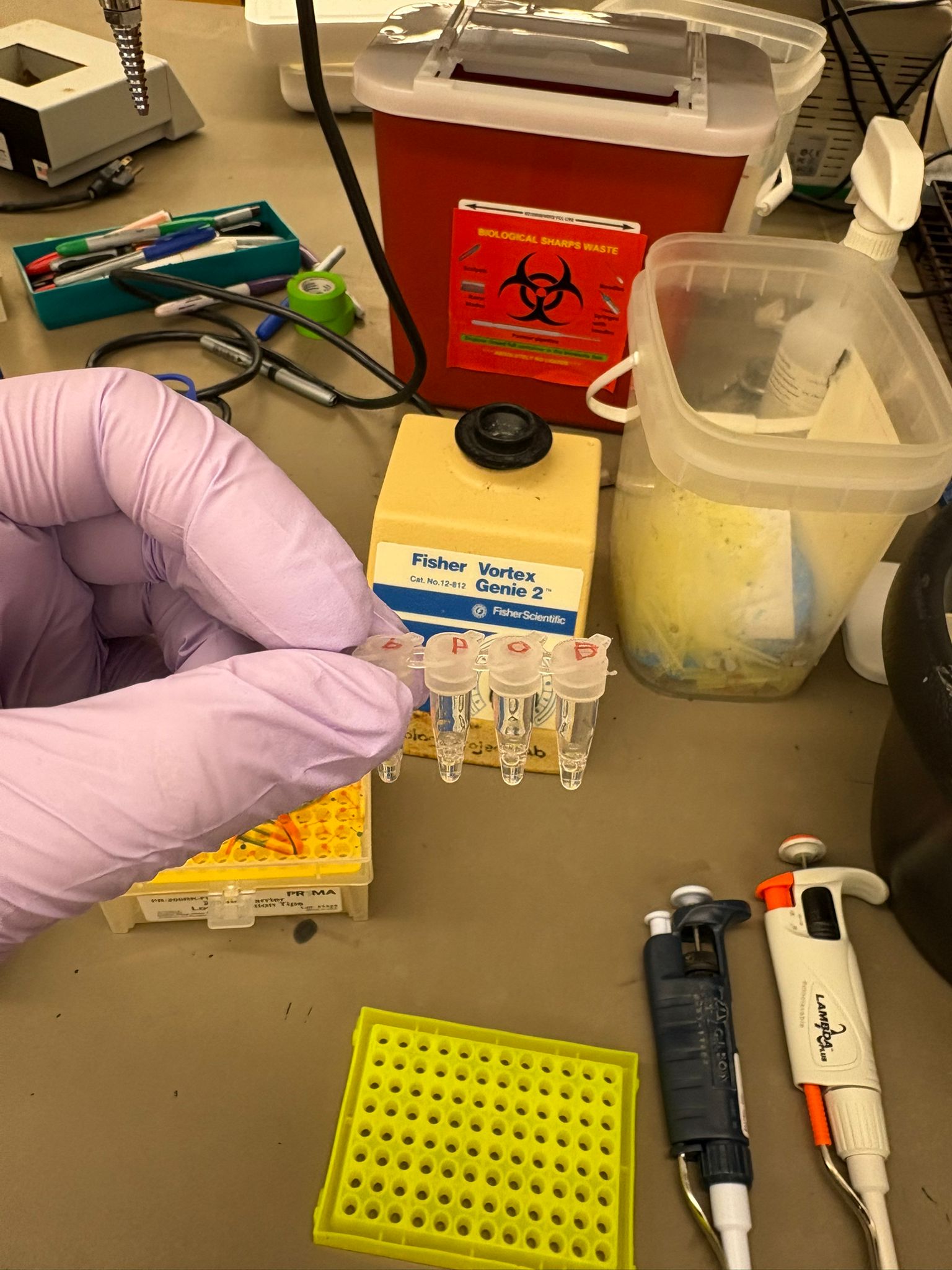
We first vortexed the PCR reactions and then prepared the samples for loading according to the following table:
| Sample | Preparation |
|---|---|
| DNA Ladder | 20 µL pre-diluted ladder |
| PCR product | 2 µL PCR product + 18 µL water |
| Original mUAV plasmid | 2 µL plasmid + 18 µL water |
| Empty wells | Fill with water |
We then ran the gel electrophoresis and obtained the following result:
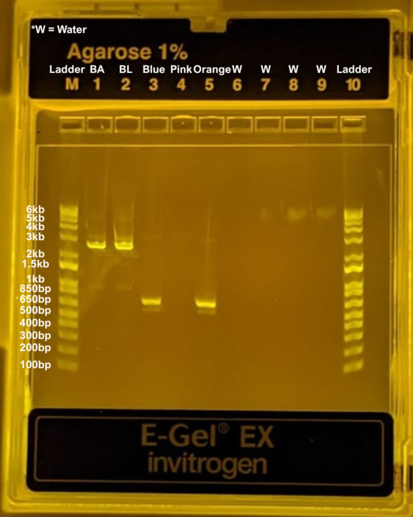
As seen in the gel, we obtained the expected fragments for the orange and blue variants, as well as for both backbone reactions (BL and BA). However, we did not observe a band in the light pink lane, suggesting that something likely went wrong during that PCR reaction. Despite this, we continued to carry the light pink sample through the rest of the protocol.
DNA Purification and Quantification
After verifying the PCR products on the gel, we proceeded with DNA cleanup using a spin-column purification kit. For each sample, we added DNA binding buffer at a 5:1 ratio relative to the PCR product volume and mixed the solution by vortexing.
The mixtures were then transferred to Zymo spin columns placed in collection tubes and centrifuged to allow the DNA to bind to the column matrix.
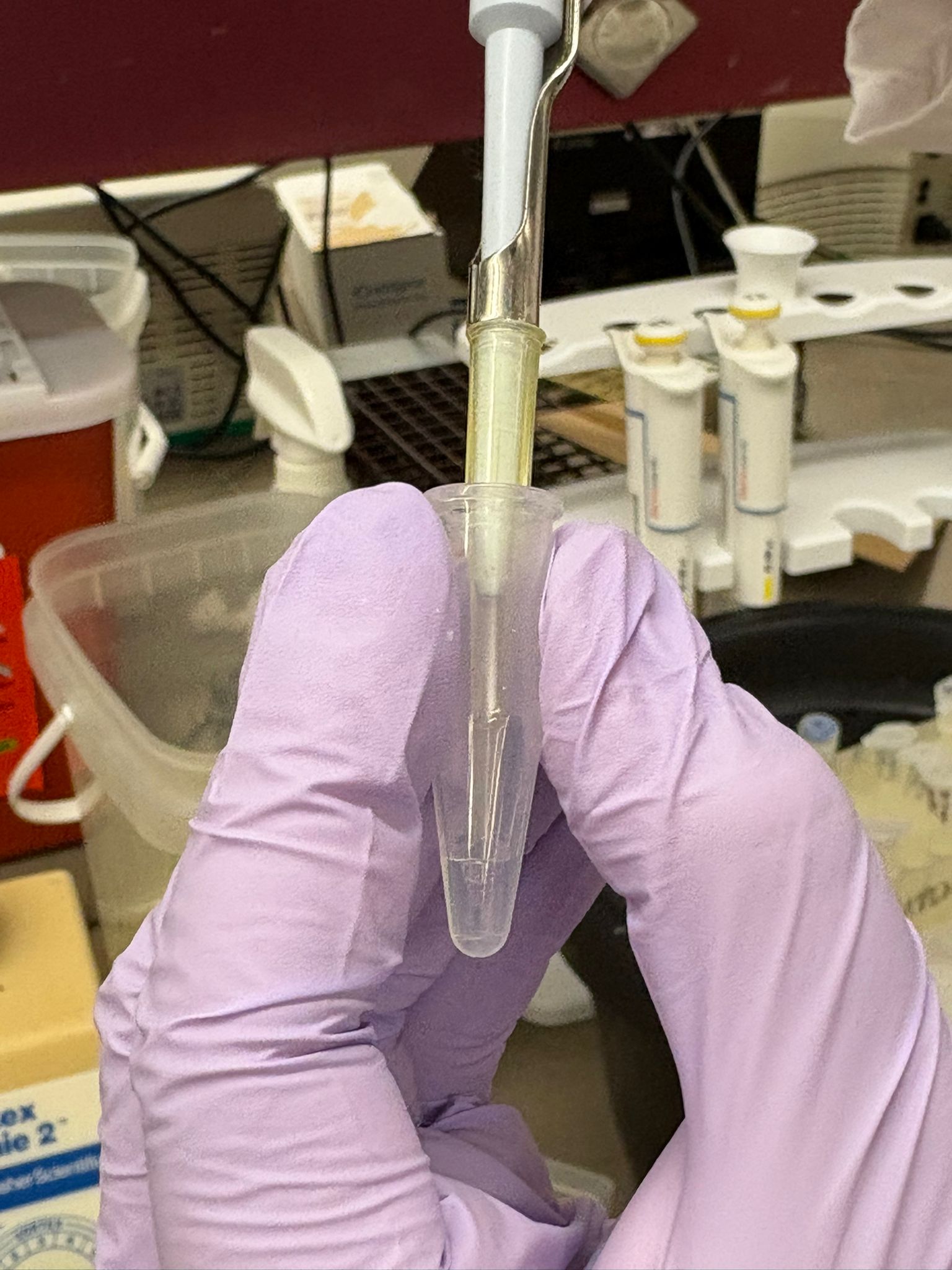
We then performed the wash step using DNA wash buffer, centrifuging after each wash and repeating this step twice to ensure proper purification of the DNA.
Finally, the DNA was eluted from the column using elution buffer, resulting in purified PCR products ready for downstream applications.
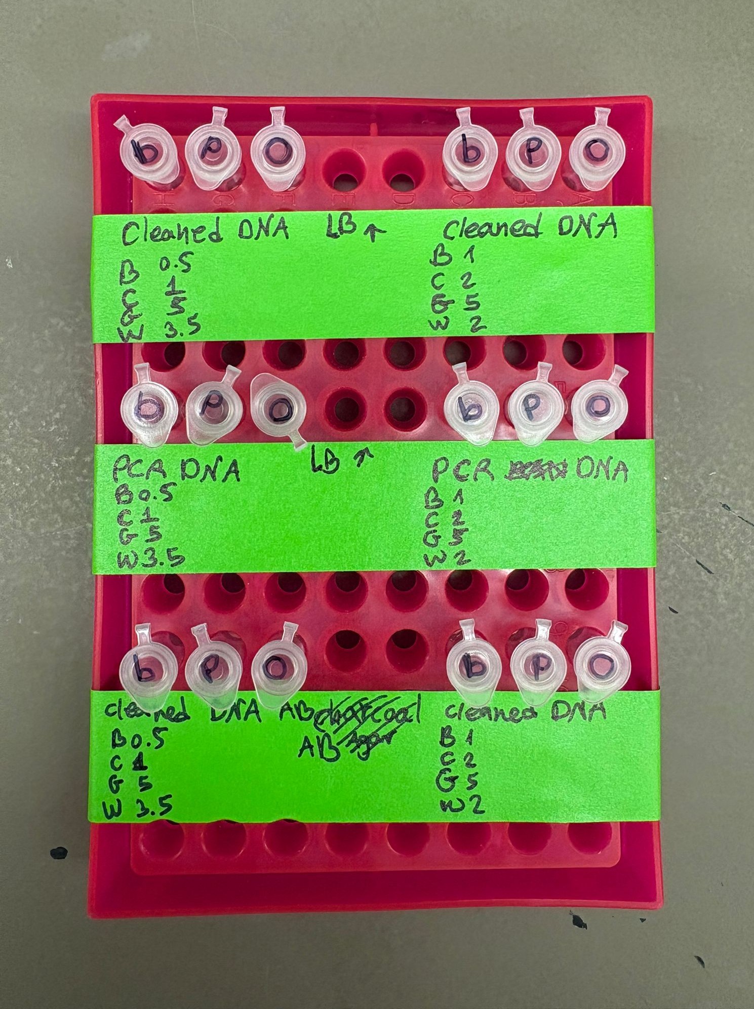
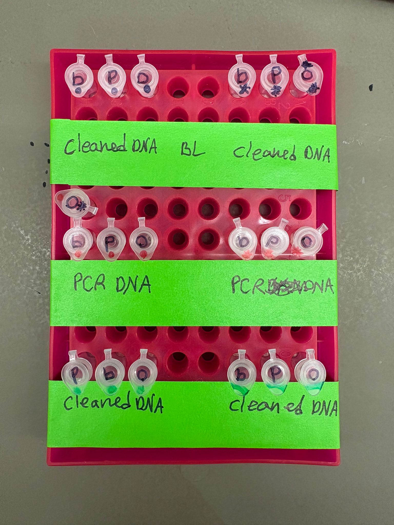
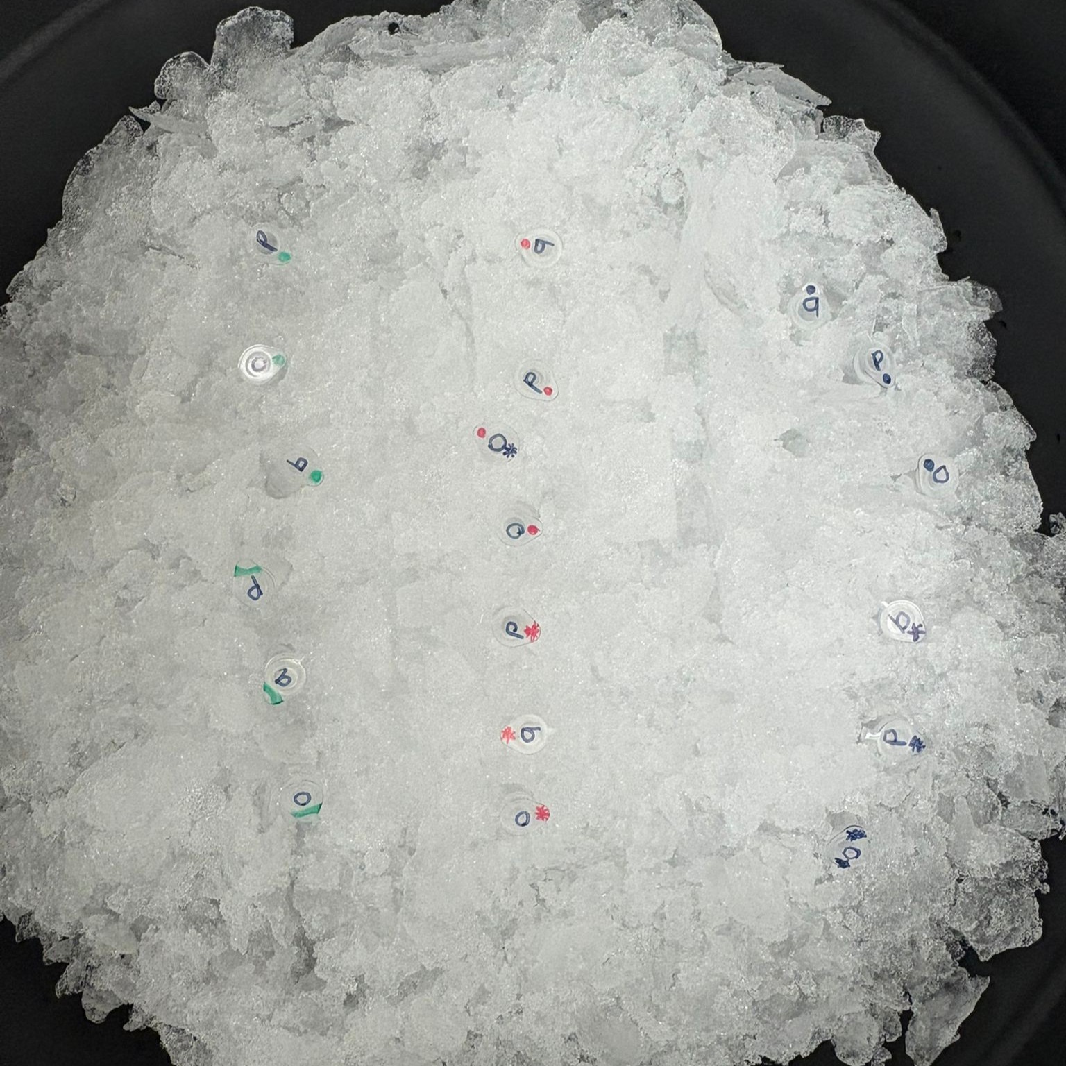
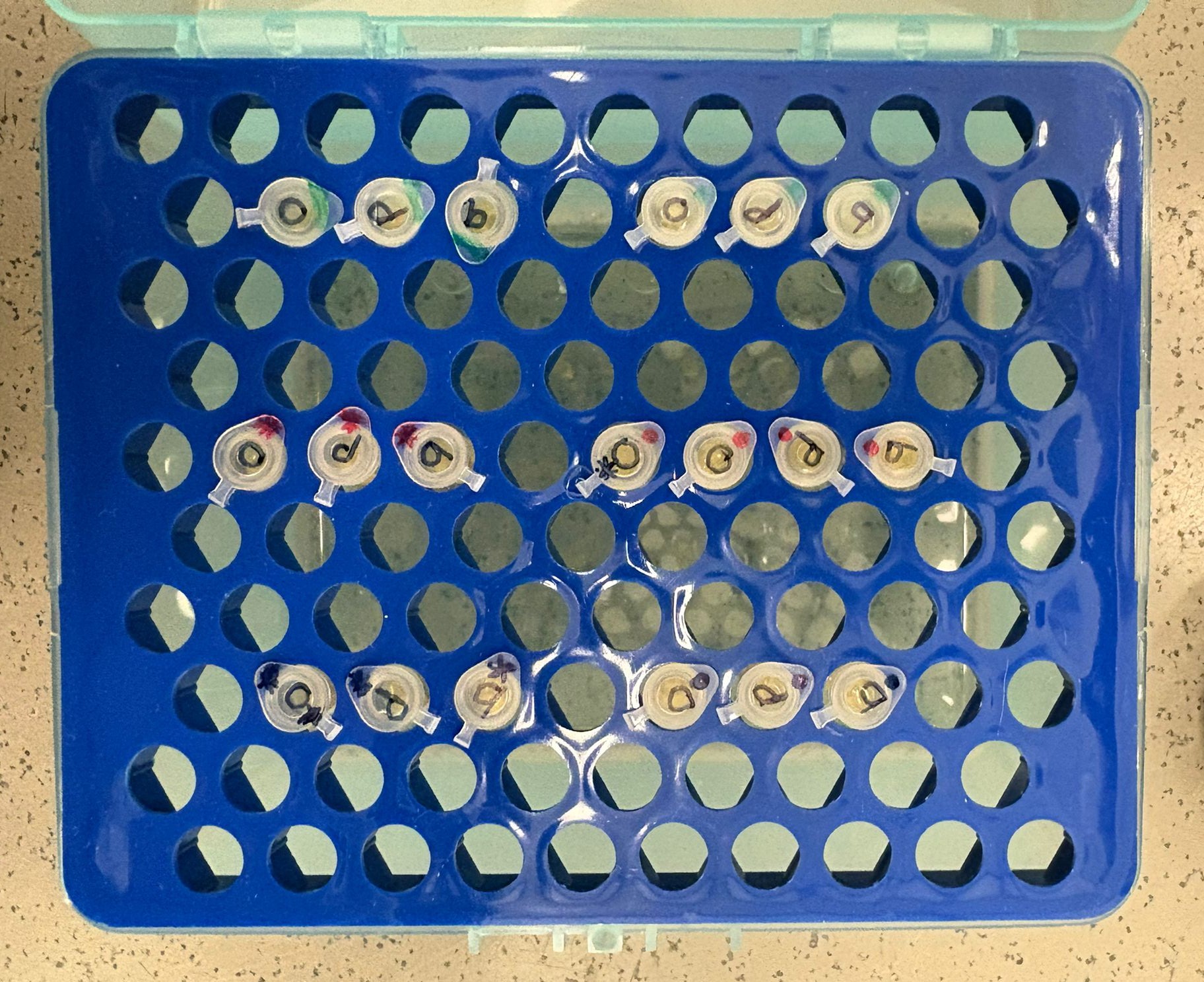
Here are the results we had at the end of the first day of this lab:
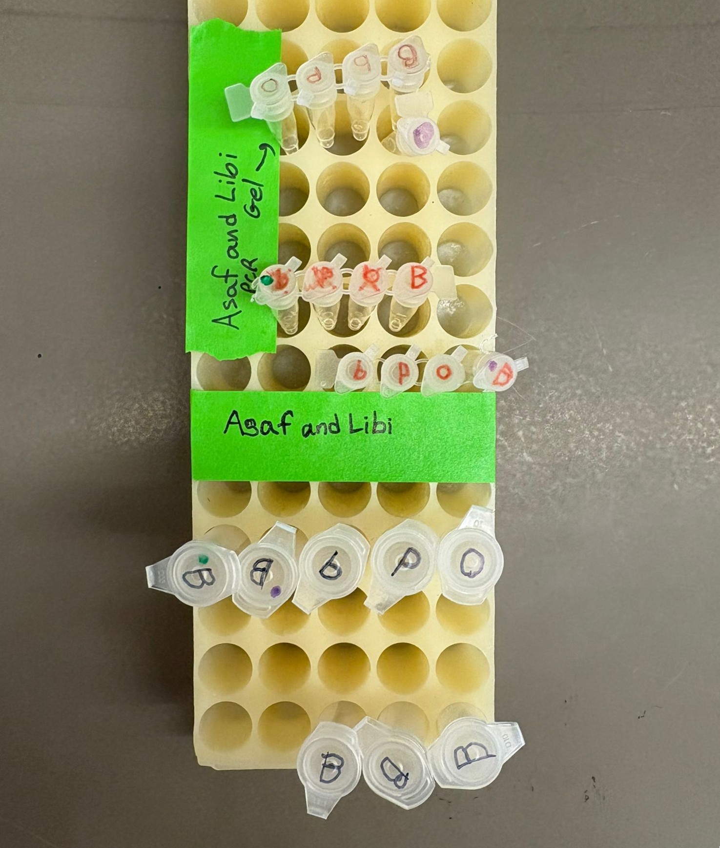
The image shows the PCR products for the three color variants and five backbone reactions, the diluted PCR products for the three colors along with BA and BL, and the cleaned PCR products for all reactions. In the labeling, BA is marked as “B” with a green dot, while BL is marked as “B” with a purple dot.
At the end of the day, we stored the purified DNA samples in the fridge and continued the experiment the following day.
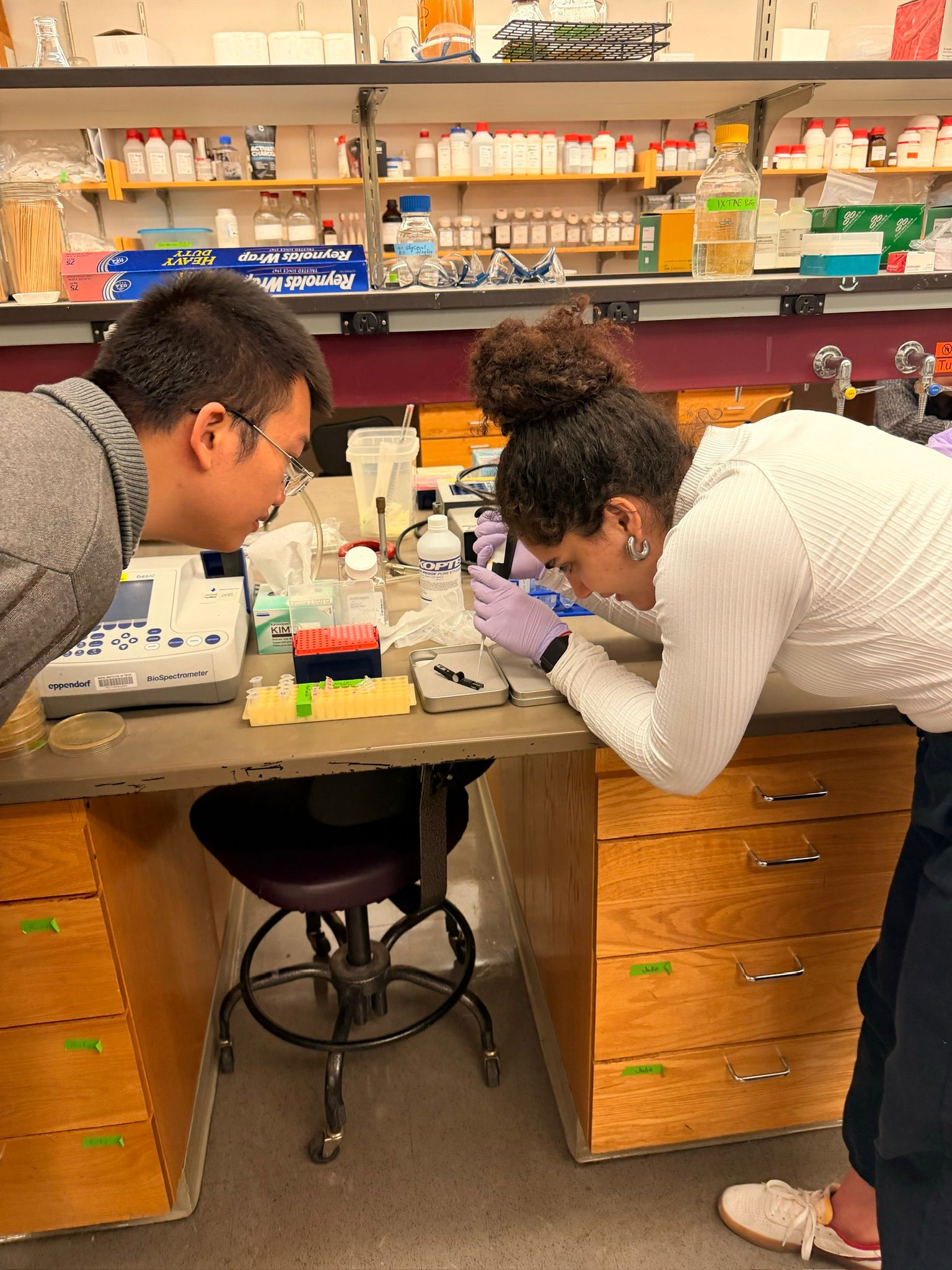
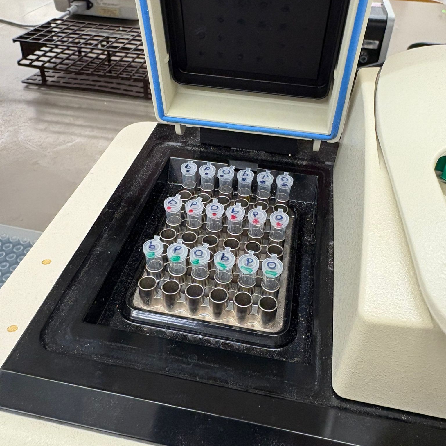
Concentration Measurement – Nanodrop
We started the second day by using a NanoDrop spectrophotometer to measure the DNA concentration of our cleaned samples. For each measurement, we loaded 2 µL of sample onto the machine.
We first measured one of the cleaned backup backbone samples and obtained the following result:
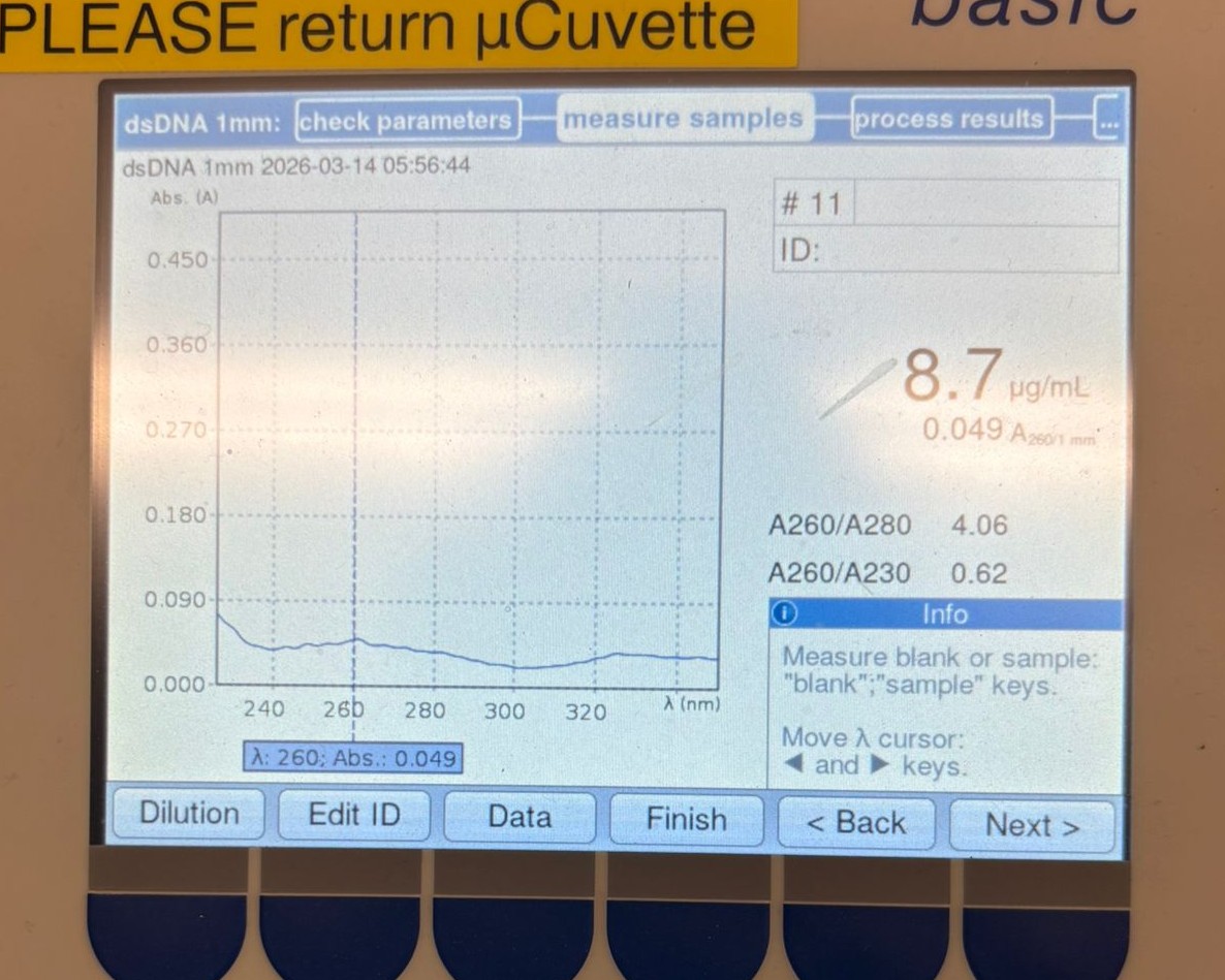
As shown, the concentration was 8.7 µg/mL, which is significantly lower than the values we expected (around ~20 µg/mL).
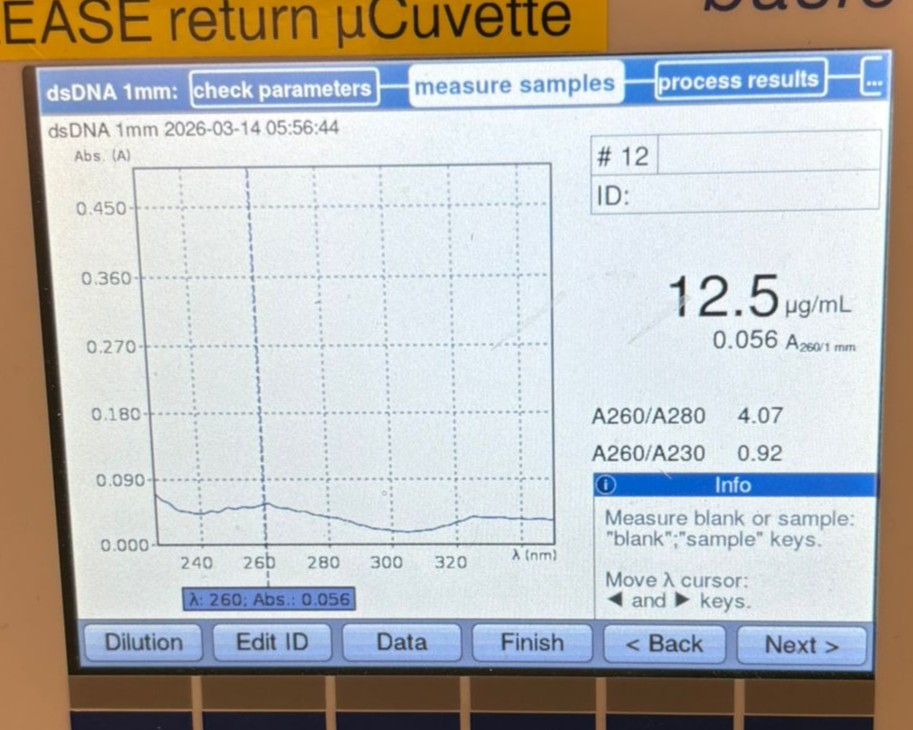
We then measured another cleaned backbone sample, this time BL, which gave a slightly better result of 12.5 µg/mL, but still lower than desired.
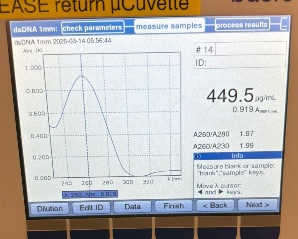
At this point, we decided to measure the concentration directly from the original PCR products (without cleanup). We first tested the BA PCR sample and obtained a much higher reading of 449.5 µg/mL:
We then measured the BL PCR sample, which showed a concentration of 486.2 µg/mL:
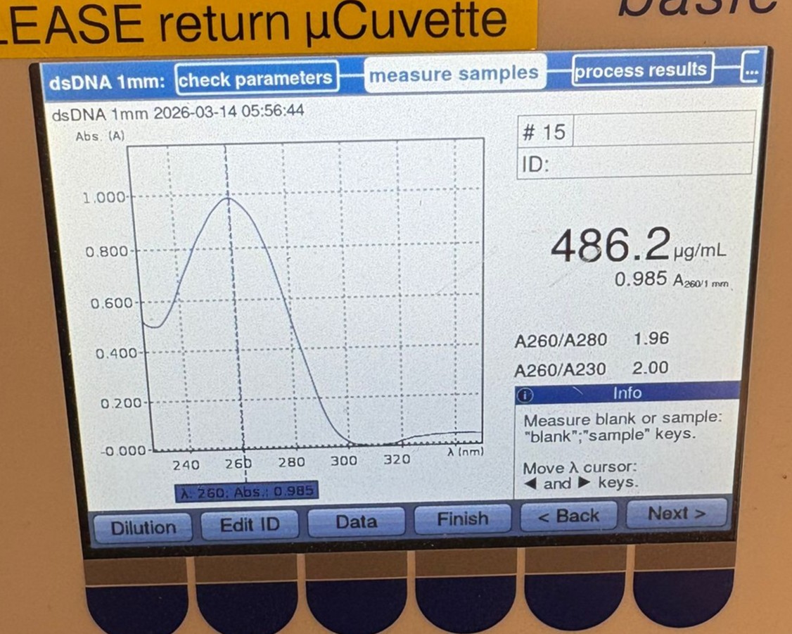
These values are likely overestimates of the true DNA concentration due to the presence of primers, nucleotides, and other components in the PCR mixture. However, they were clearly much higher than the cleaned samples, suggesting that the cleanup step may have resulted in significant DNA loss.
Gibson Assembly
For this part, we used Gibson Assembly to recombine the PCR-generated fragments into complete plasmids. We designed 6 different assemblies for each color variant (18 total), varying three main parameters:
- DNA source: cleaned vs. uncleaned PCR product (referred to as PCR)
- Backbone type: BL for PCR samples, and both BL and BA for cleaned samples
- Assembly composition: either according to the standard protocol or a modified version (x2) to compensate for the low DNA concentrations observed after cleanup
The standard assembly mixture (based on the protocol) was:
| Component | Stock Conc. (ng/µL) | Desired Conc. (ng/µL) | Volume (µL) |
|---|---|---|---|
| Backbone fragment | 50 | 25 | 0.5 |
| Insert (color fragment) | 50 | 50 | 1.0 |
| Gibson Assembly Mix | 2X | 1X | 5.0 |
| Nuclease-free water | — | — | 3.5 |
| Total | 10.0 |
To account for the low concentrations observed after cleanup, we designed a modified version (x2):
| Component | Stock Conc. (ng/µL) | Desired Conc. (ng/µL) | Volume (µL) |
|---|---|---|---|
| Backbone fragment | 50 | — | 1.0 |
| Insert (color fragment) | 50 | — | 2.0 |
| Gibson Assembly Mix | 2X | 1X | 5.0 |
| Nuclease-free water | — | — | 2.0 |
| Total | 10.0 |
All assembly combinations are summarized in the table below:
| Backbone Type | Regular Concentration | x2 Concentration |
|---|---|---|
| Clean DNA BL | 💙 🩷 🧡 | 💙 🩷 🧡 |
| PCR DNA BL | 💙 🩷 🧡 | 💙 🩷 🧡 |
| Clean DNA BA | 💙 🩷 🧡 | 💙 🩷 🧡 |
Legend:
💙 = Blue 🩷 = Light Pink 🧡 = Orange
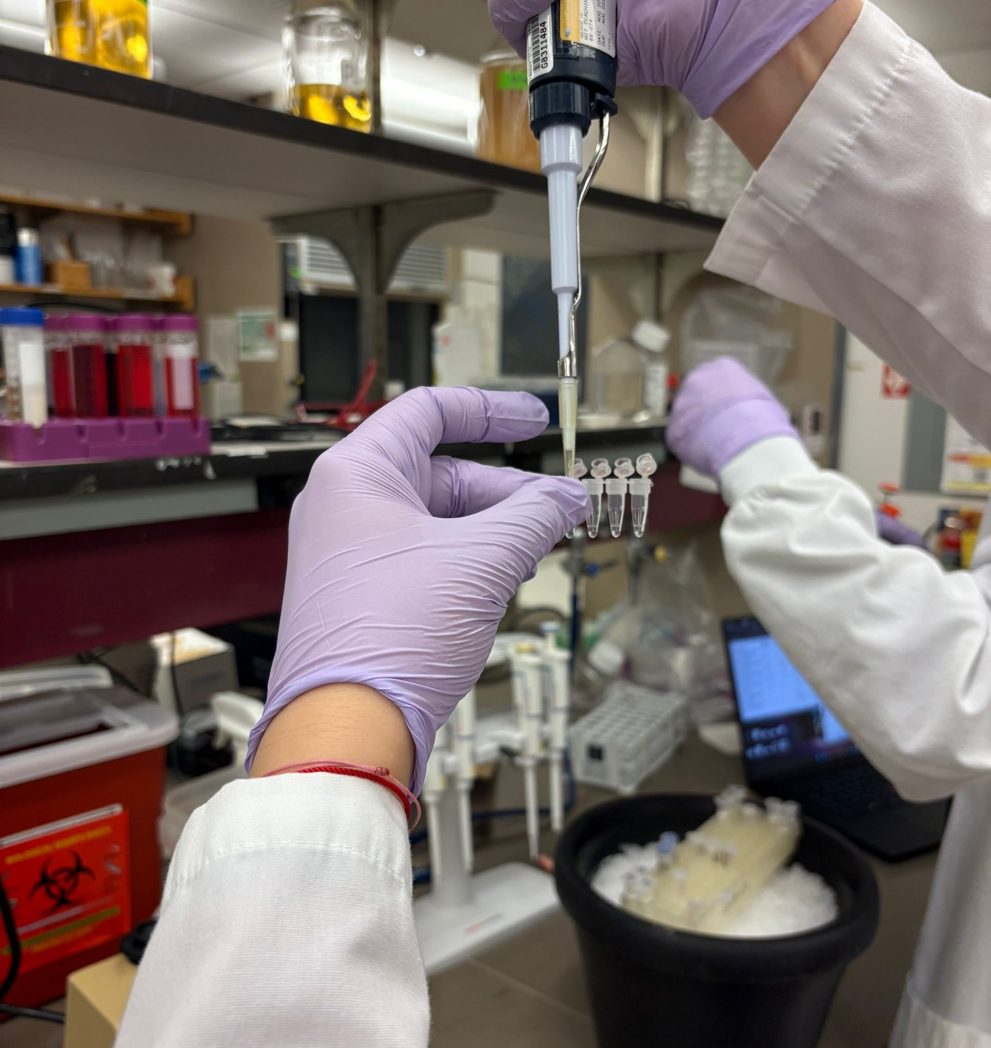
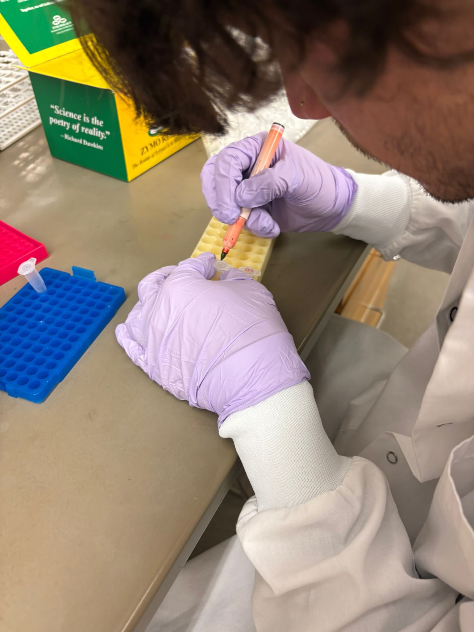
We then prepared the different assembly reactions by pipetting the required components into labeled tubes.

After preparing the mixtures, the tubes were incubated to allow the fragments to assemble into complete plasmids.
Finally, the assembled plasmids were ready for transformation into E. coli.
Transformation
For this part, we transformed the assembled plasmids into competent E. coli cells. We added the Gibson assembly products to chemically competent cells and incubated the mixtures on ice for 30 minutes to allow the DNA to associate with the cells.
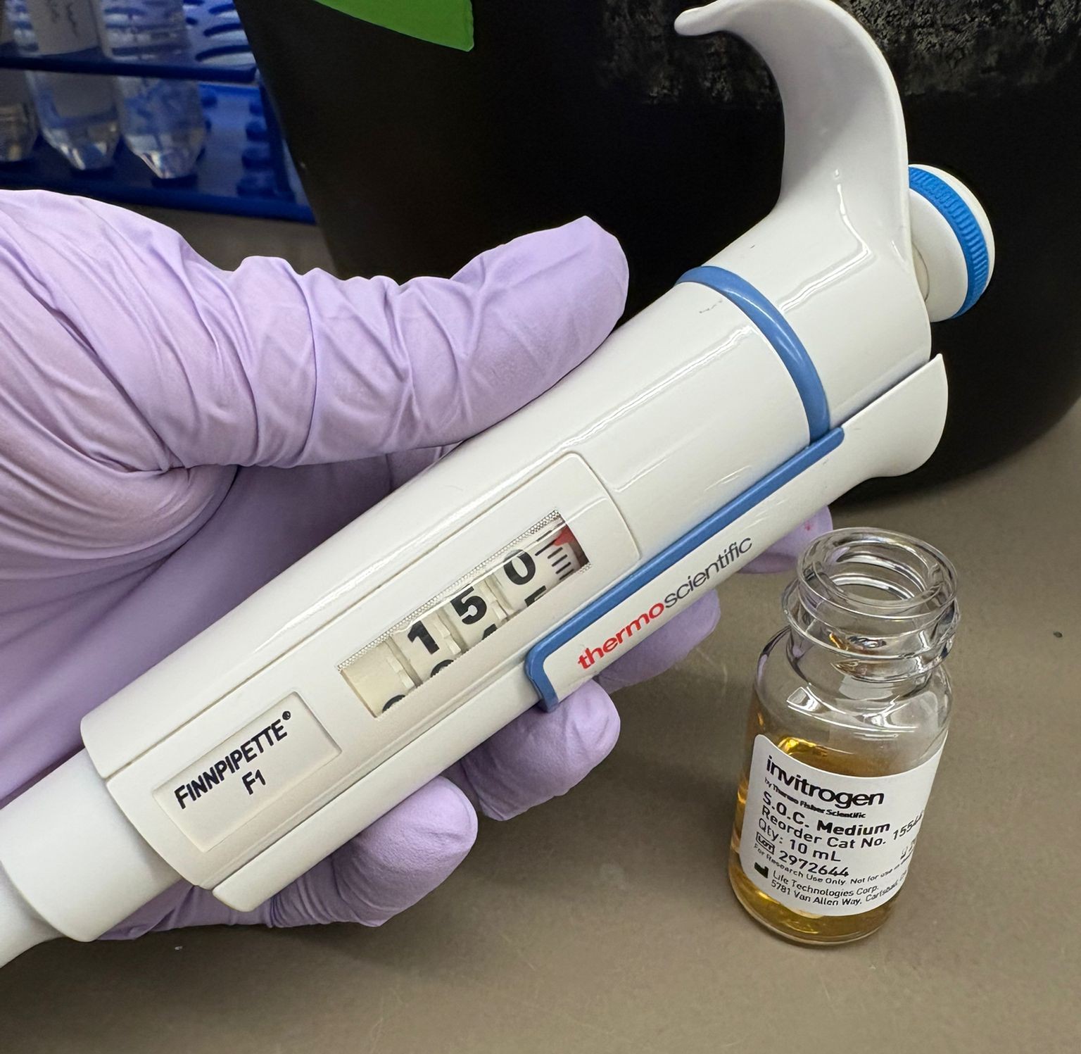
After heat shock (following the protocol), we added SOC medium to allow the cells to recover. While the protocol suggests 200–500 µL, we used 150 µL of SOC for each sample per Ronan’s reccomendation.
The tubes were then placed in a shaking incubator to promote recovery and expression of the antibiotic resistance gene.
We used standard DH5α competent cells for most transformations. However, for the orange, cleaned BL, x2 assembly, we also used 10-beta competent cells to boost transformation efficiency. In addition, we performed a separate transformation of the orange PCR BL (standard concentration) using only 10-beta cells. In total, we performed 19 transformations.
After the 60 minute growth period in the shaking incubator, we proceeded with plating the transformed cells onto agar plates.
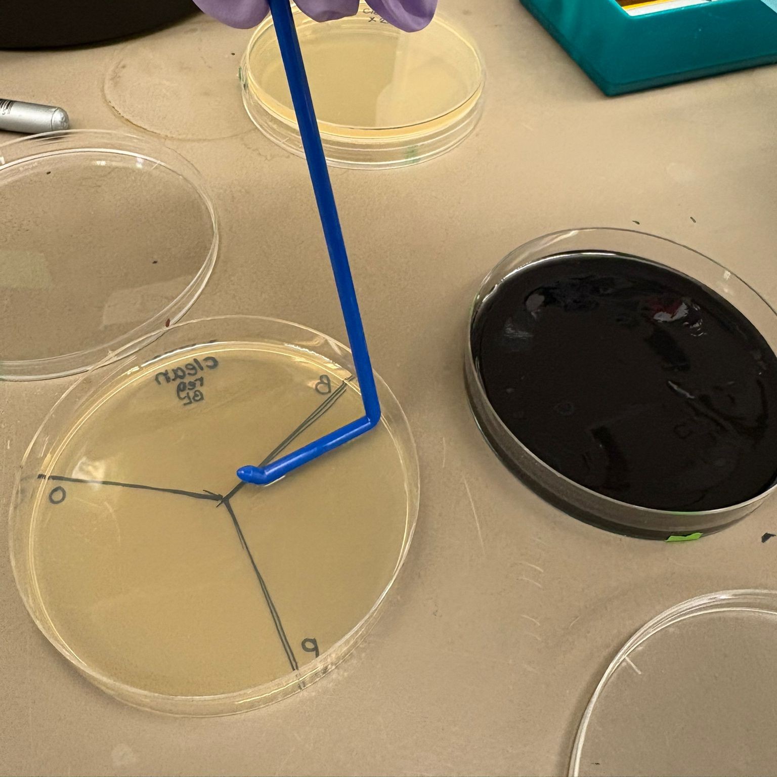
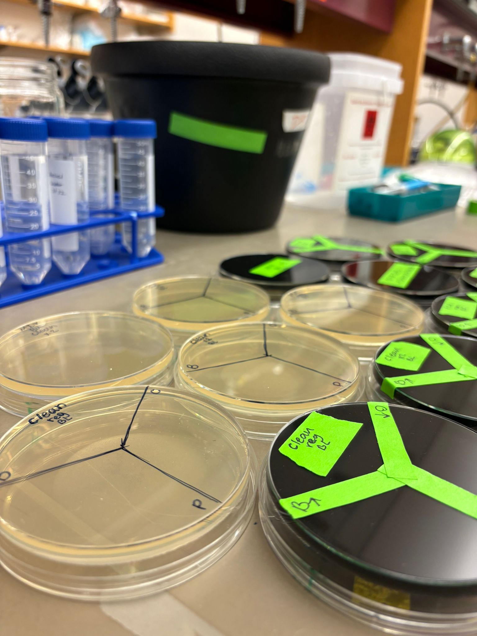
For the cleaned BL and PCR BL assemblies (both concentrations), we divided standard agar plates into thirds and plated a different color variant in each section. We also prepared a plate containing a mixture of all three colors from the BA cleaned DNA x2 assembly (we called it MIX).
We then used charcoal agar plates from the Opentrons art lab to create additional plates, since we observed some background growth on the regular plates from a control that was done earlier (colonies that likely did not take up the plasmid). We therefore wanted to use plates that we knew provide more reliable selection, and also explore the improved visual contrast offered by the charcoal medium.
For each assembly type, we again divided the plates into thirds and plated a different color in each section, this time for all assemblies. In addition, we prepared:
- A mixed plate of all three colors from the BL cleaned DNA x2 assembly
- A plate containing only the orange PCR BL (10-beta only) transformation
For plates containing all three colors, we plated 40 µL of each sample. For plates containing a single sample, we plated 100 µL.
Finally, the plates were incubated for approximately 36 hours to allow colony growth.
Results
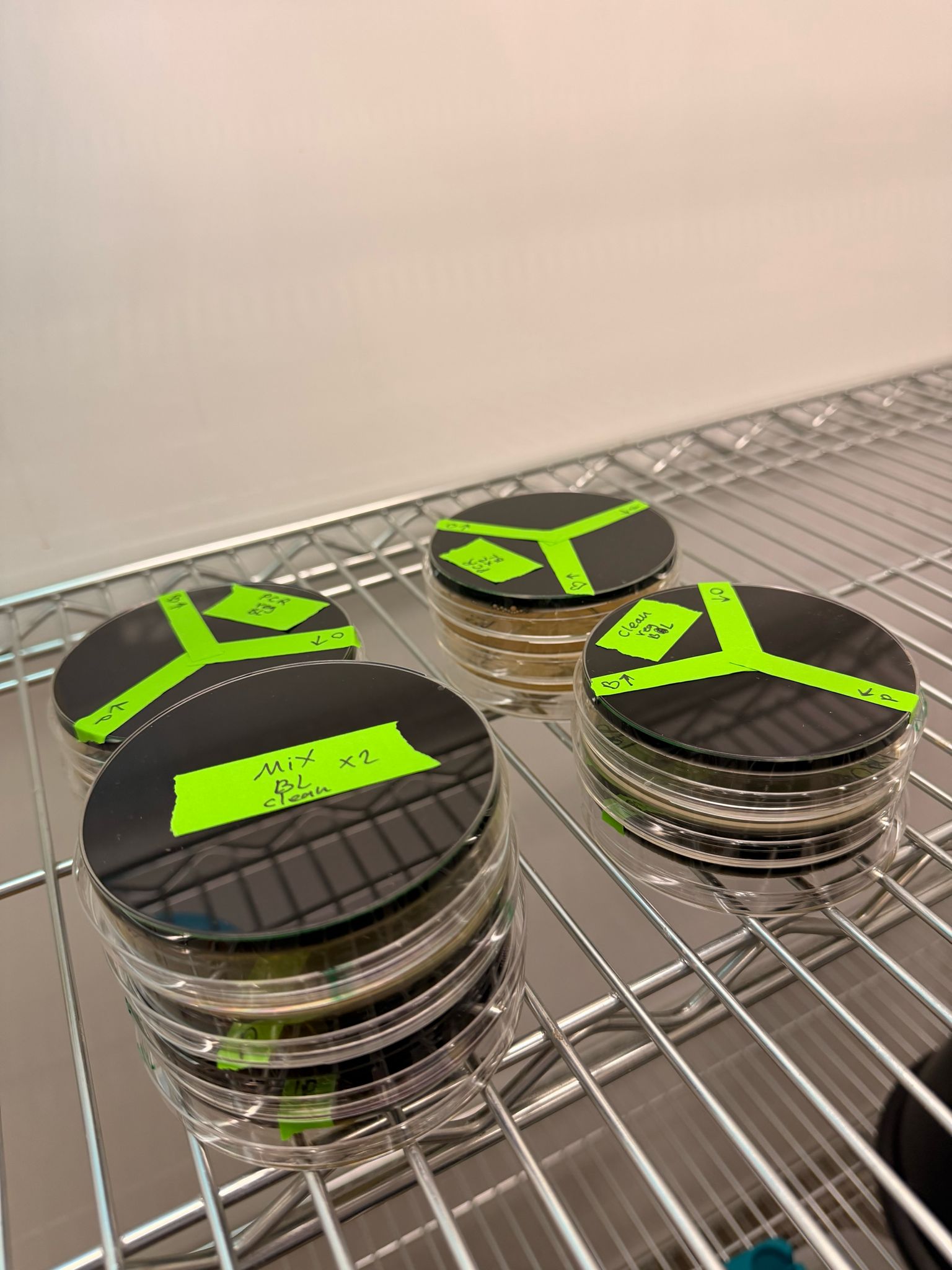
After 36 hours, the plates were taken out of the incubator and stored in the fridge.
Overall, we successfully completed the experiment. The mutation that performed best across the different assemblies was blue, followed by orange (with slightly less consistent success across plates). As expected from the gel results, the light pink variant did not appear in any of the plates, except for one potential colony on the MIX BL clean x2 plate. However, it is unlikely to be truly pink, since no corresponding signal was observed elsewhere.
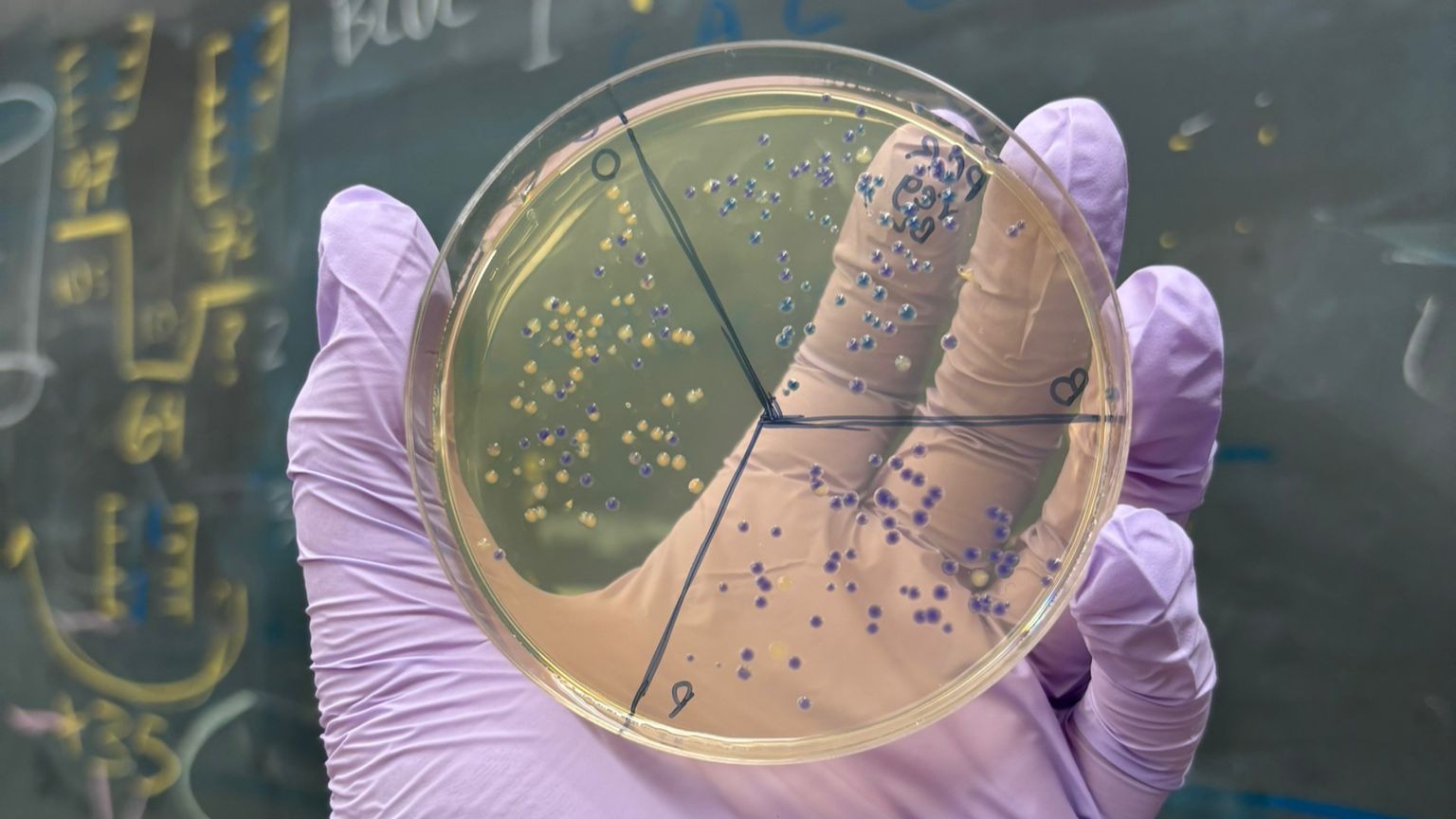
The best overall result was obtained from the PCR, regular concentration, BL assembly, which produced many clear blue and orange colonies:
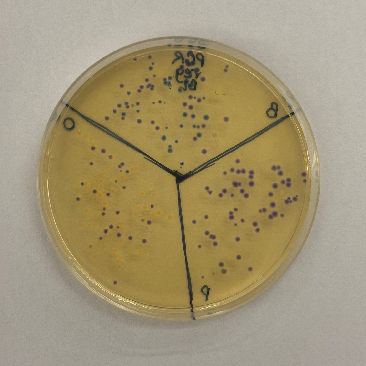
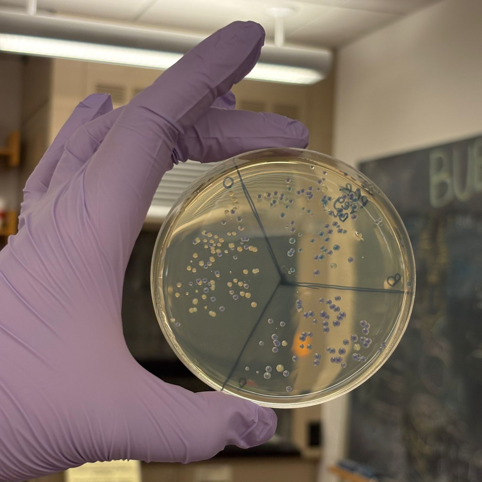
This result suggests that the uncleaned PCR samples actually performed better in the assembly, likely because they retained a much higher DNA concentration, while the cleanup step may have reduced the available DNA more than expected.
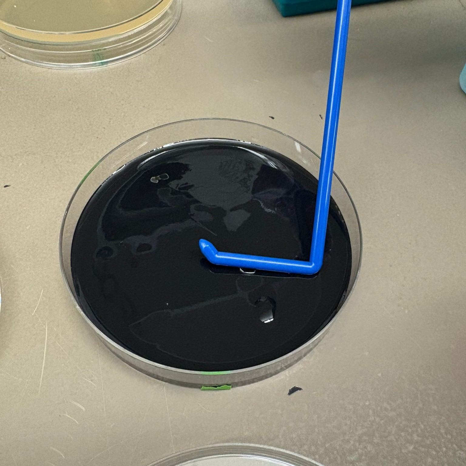
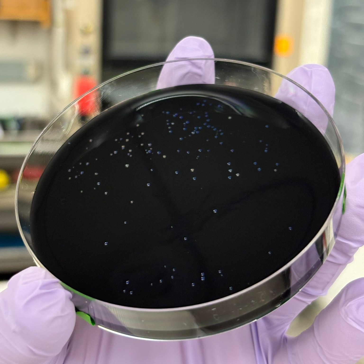
We observed slightly fewer colonies on the charcoal plates. This may suggest stronger selection conditions or differences in growth on the charcoal medium. However, these plates still provided useful results and allowed us to observe the colony colors against a dark background (although the contrast was somewhat less distinct than expected). Here as well, the best-performing condition was PCR, regular concentration, BL:
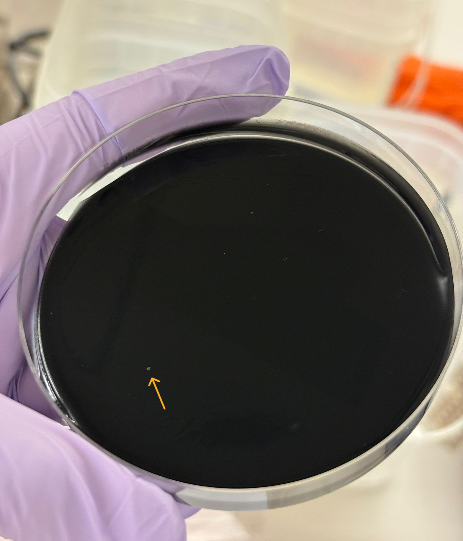
The special transformation using 10-beta competent cells for the orange variant was not successful overall, with only a single colony observed on the charcoal plate:
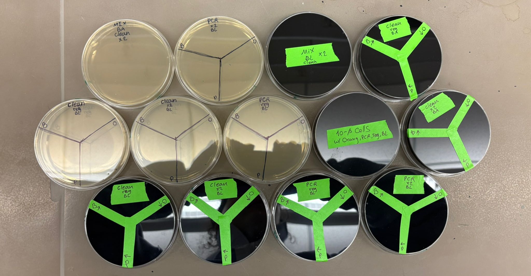
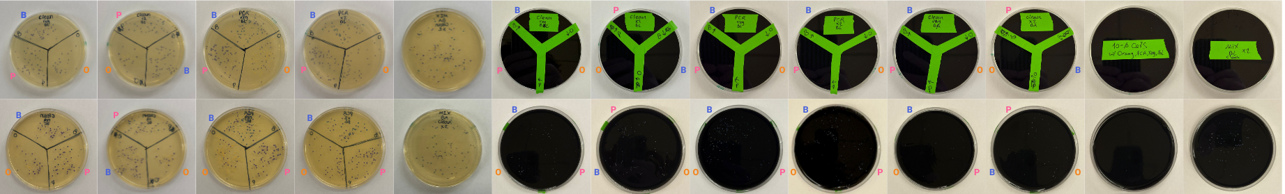
Here are the results we obtained across all plates:
Overall, this was a great experience. Seeing E. coli colonies appear in different colors was especially exciting, and it was very fun to apply techniques we had previously only learned about in theory. I’m really glad I had the opportunity to carry out this full workflow in practice.
See you next time! :)