Week 4 HW: Protein design part I
Part A. Conceptual Questions
- How many amino acid molecules are in 500 g of meat?
Ans: Average amino acid ≈ 100 Daltons (100 g/mol)
 500 g ÷ 100 g/mol = 5 moles

 1 mole = 6.022 × 10²³ molecules

 So,

 5 × 6.022 × 10²³ ≈ 3 × 10²⁴ amino acid molecules
- Why do humans eat beef but do not become a cow, eat fish but do not become fish?
Ans: When we eat beef or fish, our body breaks proteins into amino acids during digestion. Then we rebuild them into human proteins, not cow proteins.
- Why are there only 20 natural amino acids?
Ans: There are only 20 amino acids because-
 -> The genetic code evolved to encode these efficiently

 -> They provide enough chemical diversity (charge, size, polarity)

 -> Evolution kept what worked best.
- Can you make other non-natural amino acids? Design some new amino acids.
Ans: Yes, scientists can synthesize new amino acids. Example design:
 -> Add a fluorescent group → to track proteins.

 -> Add a metal-binding group → to create catalytic proteins.
- Where did amino acids come from before enzymes that make them, and before life started?
Ans: They likely formed:
 ->In the early Earth atmosphere (like in the Miller–Urey experiment)

 ->In hydrothermal vents

 ->Delivered by meteorites
Amino acids can form naturally without life.
- If you make an α-helix using D-amino acids, what handedness (right or left) would you expect?
Ams: Natural L-amino acids form right-handed helices.
D-amino acids would form a left-handed α-helix.
- Why are most molecular helices right-handed?
Ans: Most molecular helices are right-handed because life uses L-amino acids, and their 3D geometry makes right-handed helices the most stable structure.
- Why do β-sheets tend to aggregate?
Ans: They naturally stack into large sheets. Because:
 -> They form many hydrogen bonds

 -> Hydrophobic regions stick together
- Why do many amyloid diseases form β-sheets? Can you use amyloid β-sheets as materials?
Ans: In diseases like Alzheimer’s disease and Parkinson’s disease:
 ->Normal proteins misfold.

 ->Instead of staying flexible, they rearrange into β-sheet structures.

 ->β-sheets are very stable because they form many hydrogen bonds.

 ->These sheets stack together into long fibers called amyloids.

 Yes, one can use amyloid β-sheets as materials. Although harmful in disease, amyloid β-sheets have useful properties:

-> Very strong (like silk)

-> Self-assembling

-> Chemically stable

-> Nanoscale fibers
Part B: Protein Analysis and Visualization
- Briefly describe the protein you selected and why you selected it.
The protein I selected was RuBisCo from Thermosynechococcus vestitus . RuBisCO (Ribulose-1,5-bisphosphate carboxylase/oxygenase) is the key enzyme responsible for carbon fixation in photosynthesis.RuBisCO catalyzes the first major step of the Calvin cycle:
-> It adds carbon dioxide (CO₂) to ribulose-1,5-bisphosphate (RuBP).
-> This reaction produces two molecules of 3-phosphoglycerate (3-PGA).
This process allows plants, algae, and cyanobacteria to convert atmospheric CO₂ into organic molecules (sugars).
Identify the amino acid sequence of your protein.
How long is it? What is the most frequent amino acid? You can use this Colab notebook to count the frequency of amino acids.
Ans: The length is 475 amino acids , the most frequent amino acid is G. G occured 74 times in the sequence.
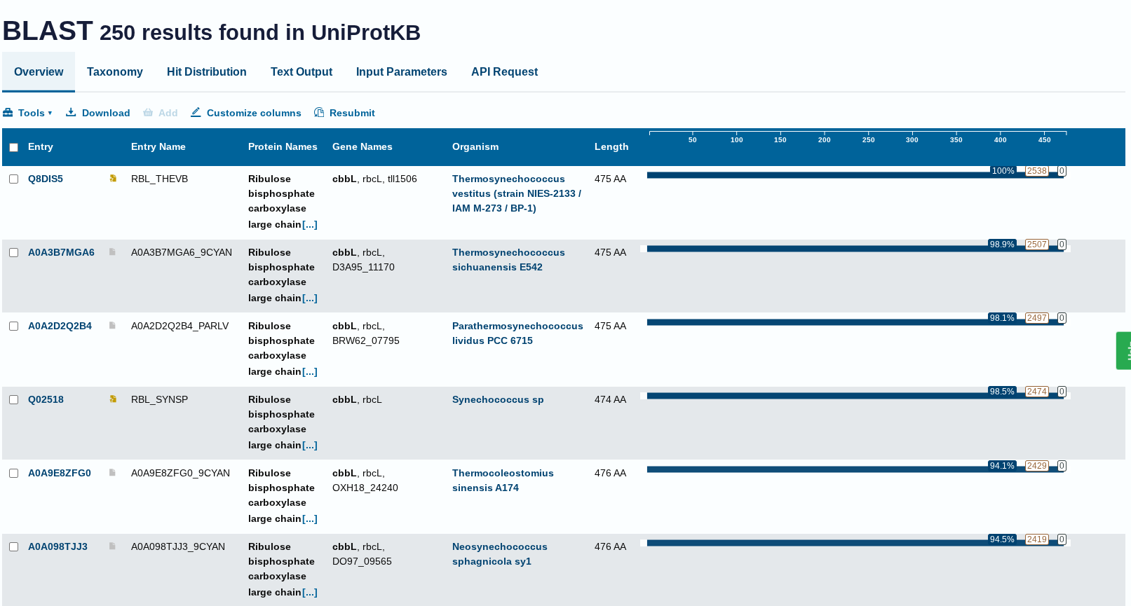
How many protein sequence homologs are there for your protein? Hint: Use Uniprot’s BLAST tool to search for homologs.
Ans: There 250 homologs to the protein- RuBISCo
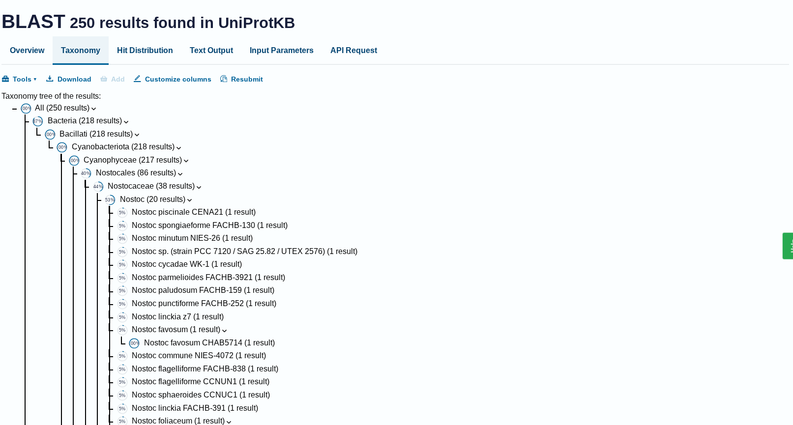
Does your protein belong to any protein family?
Ans: Belongs to the RuBisCO large chain family. Type I subfamily.
Identify the structure page of your protein in RCSB
When was the structure solved? Is it a good quality structure? Good quality structure is the one with good resolution. Smaller the better (Resolution: 2.70 Å)
Ans: The structure was experimentally solved using X-ray diffraction data collected on February 4, 2007.
 So the timeline is:

 ->Data collected (structure solved): 2007-02-04

 ->Deposited to Protein Data Bank: 2011-03-10

 ->Released publicly: 2012-03-28

 Yes, it is a good quality structure, the resolution is 2.30 Å

 Are there any other molecules in the solved structure apart from protein?

 Ans: Yes, there are Cl ligand present in the solved structure. Along with the ligand water molecules and ions are present, these comes under hetero molecules.

 Does your protein belong to any structure classification family?

 Ans: Yes, my protein is structurally classified and is part of the RuBisCO small subunit structural family.
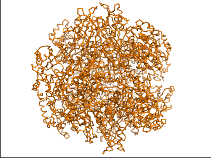
Open the structure of your protein in any 3D molecule visualization software:
PyMol Tutorial Here (hint: ChatGPT is good at PyMol commands)
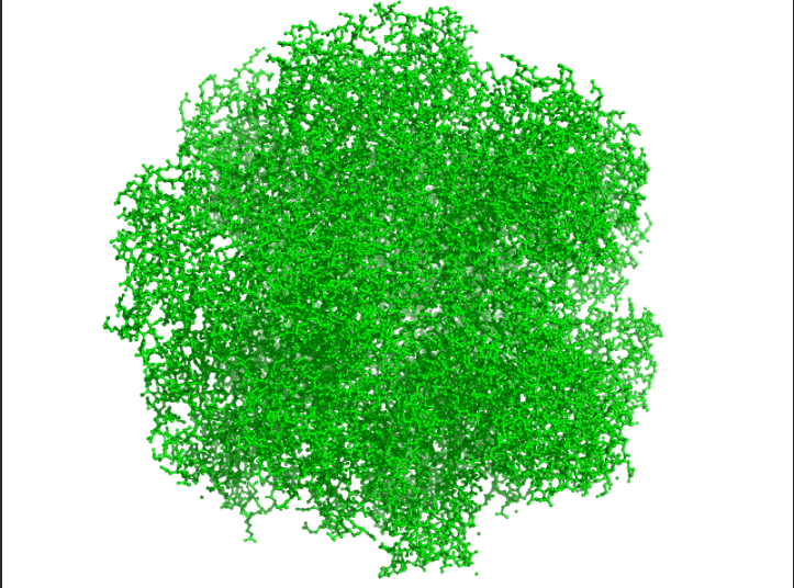
Visualize the protein as “cartoon”, “ribbon” and “ball and stick”.
Ans: The protein structure was visualized using cartoon, ribbon, and ball-and-stick representations. The cartoon and ribbon models highlight the overall fold and secondary structural elements, while the ball-and-stick model shows atomic-level details of the protein structure.
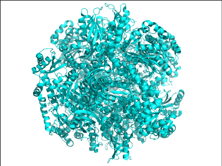
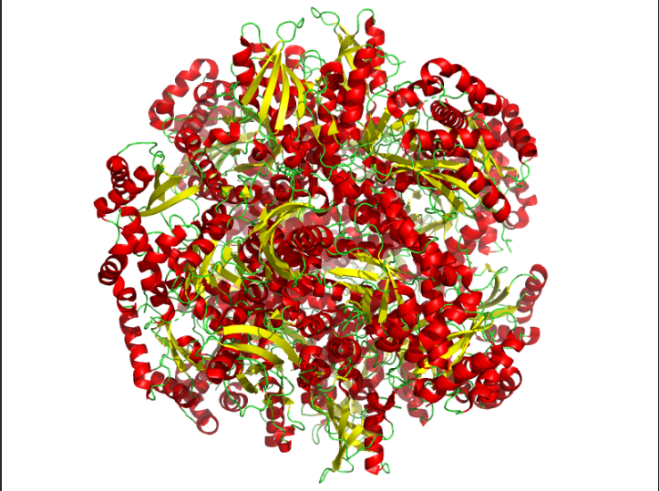
Color the protein by secondary structure. Does it have more helices or sheets?
Ans: The protein is predominantly β-sheet(yellow) rich with fewer α-helices(red).
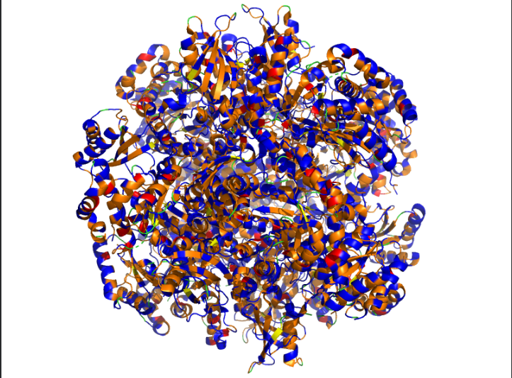
Color the protein by residue type. What can you tell about the distribution of hydrophobic vs hydrophilic residues?
Ans: Hydrophobic(orange) residues are buried in the core, while hydrophilic(yellow) residues are exposed on the surface, consistent with a soluble enzyme.
Visualize the surface of the protein. Does it have any “holes” (aka binding pockets)?
Ans: Surface representation reveals shallow binding pockets and structural clefts that likely contribute to substrate binding and subunit interaction.
Part C. Using ML-Based Protein Design Tools
C1. Protein Language Modeling
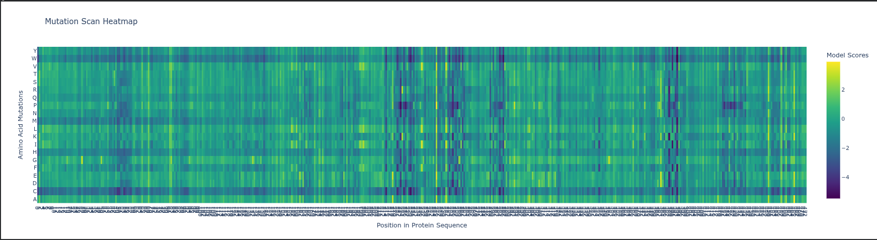
Deep Mutational Scan (DMS) ESM2 Likelihoods: The heatmap predicts how a mutation affects protein fitness by calculating how the model is by a change; high negative values (darker colors) indicate mutations that likely disrupt the protein’s structure or function.
Specific Pattern: Look at Glycine (G) or Proline (P) residues in the sequence; mutations at these sites usually stand out as highly deleterious (darker) because these amino acids have unique structural roles (flexibility or rigid kinks) that other residues cannot easily replace.
Experimental Comparison: In RuBisCO, ESM2 predictions generally correlate strongly with experimental data in the catalytic core, but the model may “under-predict” the impact of mutations in surface loops that are functionally important for protein-protein interactions (like with RuBisCO activase) but less evolutionarily conserved.
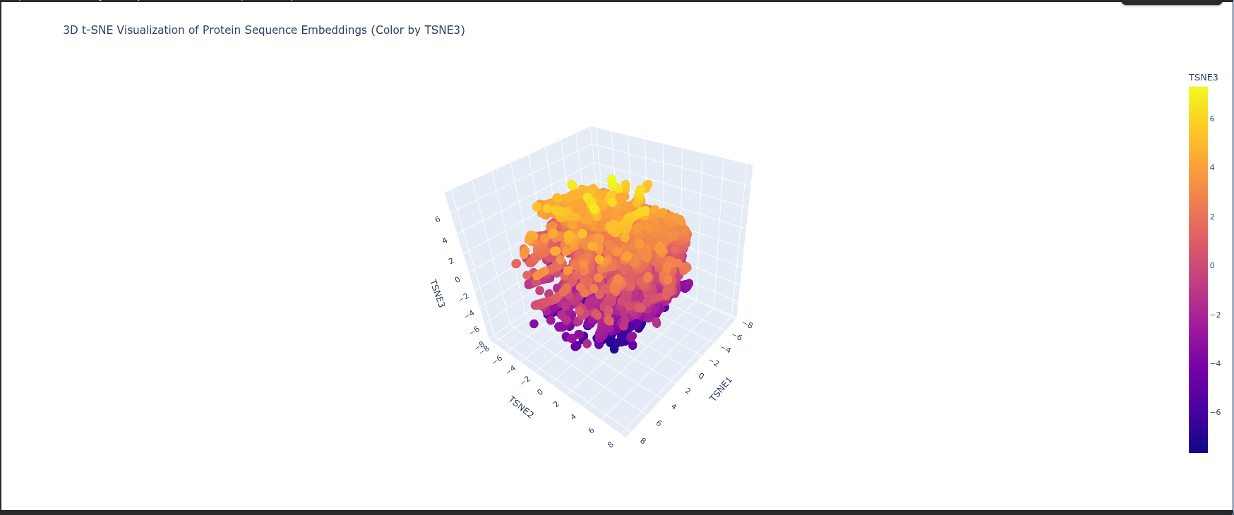
Latent Space Analysis Neighborhoods: The clusters in t-SNE plot represent groups of proteins with similar structural folds and evolutionary origins, meaning proteins in the same neighborhood likely share the same biological pathway or enzymatic mechanism.
Protein Position: The protein is positioned based on its high-dimensional embedding; it likely sits in a dense neighborhood of Type I RuBisCO enzymes, indicating it shares a highly conserved sequence identity and 3D architecture with other photosynthetic large subunits.
Similarity: Proximity to neighbors suggests that ESM2 has successfully captured “hidden” biological rules—such as hydrophobic packing and electrostatic networks—placing the protein near those with the most similar functional constraints.
C2. Protein Folding
Protein Folding Analysis Coordinate Matching: ESMFold predictions generally match original structures closely for well-defined domains, though disordered regions show higher variance between predicted and experimental coordinates.
Structural Resilience: The protein appears highly resilient to single mutations, as most of the heatmap is green (neutral), indicating that the language model expects the overall fold to remain stable despite small changes.
Segment Impact: Large segment deletions or radical mutations in the “dark blue” caused structural collapse, as these regions represent the core stability of the protein.
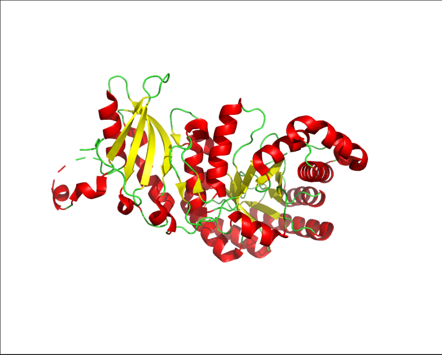
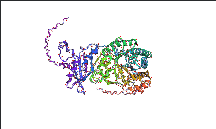
The image depicts the structure of the protein RuBISCo
C3. Protein Generation
The predicted sequence has low score when compared to the original sequence. Below images show structural difference between predicted sequence and original sequence.
Image depicts the structure of original sequence
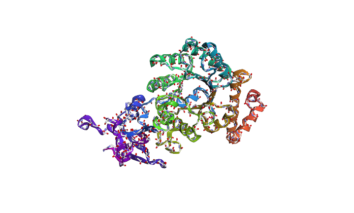
Image depicts the structure of predicted sequence.
Part D. Group Brainstorm on Bacteriophage Engineering
Find a group of ~3–4 students
Read through the Phage Reading material listed under “Reading & Resources” below.
Review the Bacteriophage Final Project Goals for engineering the L Protein:
Increased stability (easiest)
Higher titers (medium)
Higher toxicity of lysis protein (hard)
Brainstorm Session
Choose one or two main goals from the list that you think you can address computationally (e.g., “We’ll try to stabilize the lysis protein,” or “We’ll attempt to disrupt its interaction with E. coli DnaJ.”).
Write a 1-page proposal (bullet points or short paragraphs) describing:
Which tools/approaches from recitation you propose using (e.g., “Use Protein Language Models to do in silico mutagenesis, then AlphaFold-Multimer to check complexes.”).
Why do you think those tools might help solve your chosen sub-problem?
Name one or two potential pitfalls (e.g., “We lack enough training data on phage–bacteria interactions.”).
Include a schematic of your pipeline.
This resource may be useful: HTGAA Protein Engineering Tools
Each individually put your plan on your HTGAA website
- Include your group’s short plan for engineering a bacteriophage
Answers
Our group proposes to computationally engineer the MS2 bacteriophage L protein with two primary goals:
- Increased Stability
Redesign the N-terminal and transmembrane domains to reduce proteolytic degradation and improve protein accumulation in the host membrane.
- Increased Toxicity
Optimize lytic kinetics so that the L protein bypasses or weakens the DnaJ-dependent damping mechanism, allowing faster host cell lysis.
We selected these goals because both can be explored computationally through sequence generation, mutational analysis, and structural modeling before experimental validation.
Proposed Computational Pipeline
- Generative Sequence Design – Evo 2
Approach:
- We will use Evo 2 to generate a library of new MS2 L protein variants.
We will focus on:
modifying or truncating the N-terminal Domain 1
generating Lodj-like variants that may reduce DnaJ interaction
exploring mutations beyond naturally observed variants
Why this helps:
- Evo 2 can explore sequence space beyond known phage evolution and may suggest variants with stronger lysis activity or improved accumulation.
- Sequence Stability Optimization – ProteinMPNN
Approach:
- Use ProteinMPNN on the transmembrane domain (TMD) of candidate sequences.
Focus:
preserve membrane insertion geometry
improve folding stability
reduce destabilizing mutations
Why this helps:
- The L protein depends on proper membrane insertion. Stable folding in the TMD should improve accumulation and make lysis more reliable.
- Functional Motif Tuning – ESM-2 / ESM-3
Approach:
- Use ESM-2 and ESM-3 for in silico mutagenesis around the Leu48–Ser49 (LS) motif.
Focus:
test substitutions around conserved residues
evaluate sequence embeddings
preserve functional amino acid properties while improving toxicity
Why this helps:
- The LS motif is central to L protein function. Language models can estimate which mutations remain biologically plausible while potentially improving activity.
Oligomerization Verification – AlphaFold-Multimer
Approach:
- Use AlphaFold-Multimer to predict oligomeric assembly.
Focus:
- ability to form 10-mer or higher clusters
- membrane pore geometry
- mutation effects on assembly interfaces
Why this helps:
- The MS2 L protein lyses cells by clustering in membranes. Structural prediction helps identify variants likely to assemble correctly.
Potential Pitfalls
- Over-toxicity / premature lysis
If engineered L proteins trigger lysis too early, E. coli may burst before the phage completes replication.
Possible consequence:
- faster lysis, but lower phage production
- Membrane protein prediction limitations
Many protein prediction models perform better on soluble proteins than membrane proteins.
Possible issue:
predicted oligomers may differ from real membrane behavior
lipid bilayer effects may not be captured accurately
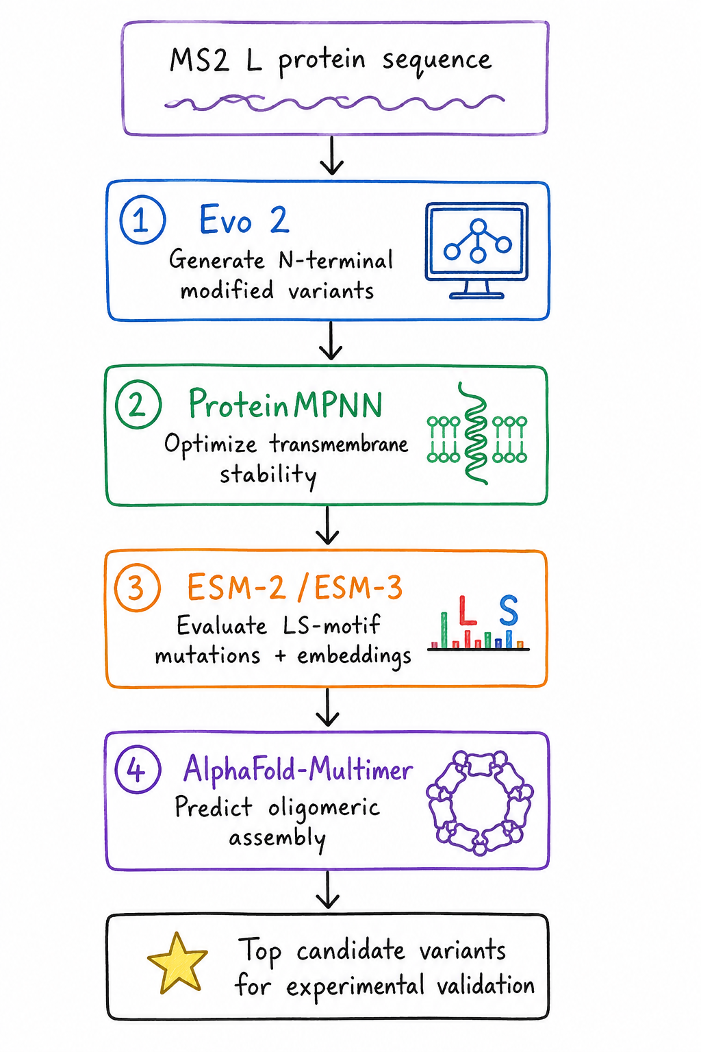
Proposed computational workflow for engineering the MS2 L protein, integrating sequence generation, stability optimization, mutational analysis, and structural prediction to identify promising variants for experimental validation.
Short Group Plan
Our group will computationally engineer the MS2 bacteriophage L protein for greater stability and stronger lytic activity.
We will combine:
generative sequence design
protein language models
inverse folding
structure prediction
To identify promising L protein variants that:
- accumulate more effectively in membranes
- maintain functional oligomerization
- potentially bypass DnaJ damping for faster lysis
These candidates would then be prioritized for future experimental testing.