Week 1 HW: Principles and Practices

Bioindicator for Microplastic Contamination in Agricultural Soils

1. Biological Engineering Application

Project Description

The proposed biological engineering application is the development of a bioindicator for detecting contamination by microplastics and their chemical additives in agricultural soils.

The system would be based on a genetically modified soil bacterium (Pseudomonas spp.), a microorganism naturally associated with the rhizosphere of crops such as:

• Maize
• Wheat

Functional Concept

The engineered bacterium would be designed to:

• Detect stress caused by microplastic additives present in soil
• Produce a visible signal (e.g., fluorescence) when exposed to such stress

This mechanism would enable:

• Early detection of soil contamination
• Identification of potential stress conditions affecting crops
• On-site monitoring without exclusive reliance on laboratory-based analytical methods

Motivation

Microplastics are increasingly present in agricultural soils due to multiple sources, including agricultural plastics and contaminated inputs. Current detection methods are:

• Technically complex
• Costly
• Primarily limited to laboratory analysis

This project aims to provide a field-deployable, cost-effective biological monitoring tool to complement existing analytical techniques.

Governance and Policy Framework

2. Governance and Policy Goals

The following goals guide the evaluation of governance actions for this project.

Biosecurity

Ensure that the use of a genetically modified microorganism as a bioindicator:

• Does not create biological or environmental risks

• Protects sustainable soil use

• Avoids negative impacts on:

  • Soil ecosystems
  • Crops (maize and wheat)
  • Non-target organisms

Ethics

Ensure responsible and socially acceptable use of the technology by:

• Protecting local communities
• Promoting transparency
• Limiting the application strictly to environmental monitoring purposes

Other Considerations

• Ensure technical feasibility
• Consider economic costs
• Minimize burdens to stakeholders
• Avoid unnecessary impediments to scientific research
• Promote constructive and responsible applications of biotechnology

3. Potential Governance Actions

Action 1: Environmental Biosecurity Assessment Before Field Use

• Type: Regulatory requirement
• Actors: Academic researchers, environmental regulators

Purpose

Require a formal environmental biosecurity assessment prior to field application in order to prevent biological and ecological risks in agricultural soils.

Design

• Researchers prepare risk assessment protocols
• Regulatory or institutional bodies review and approve these protocols before field testing

Assumptions

• Laboratory experiments can reasonably predict environmental behavior and associated risks

Risks of Failure

• Long-term environmental effects may be underestimated

Risks of Over-Strict Implementation

• Excessively strict requirements may slow down research and innovation

Action 2: Technical Biological Containment Strategies

• Type: Technical strategy
• Actors: Researchers, technology developers

Purpose

Reduce environmental risks by limiting the survival or activity of the bioindicator microorganism outside controlled soil conditions.

Design

• Genetic containment mechanisms are incorporated during the design stage
• Containment is built directly into the microorganism’s genetic architecture

Assumptions

• Containment systems are stable and effective
• Containment does not significantly reduce bioindicator performance

Risks of Failure

• Containment mechanisms fail under real environmental conditions

Risks of Over-Strict Implementation

• Excessive biological control reduces detection sensitivity or functionality

Action 3: Transparency and Engagement with Local Farming Communities

• Type: Ethical governance / incentive mechanism
• Actors: Researchers, institutions, farmers

Purpose

Ensure ethical and socially responsible implementation by informing and engaging farming communities.

Design

• Provide clear information regarding:

  • Purpose of the bioindicator
  • Operational limits
  • Potential risks

• Involve local communities in decision-making processes

Assumptions

• Transparency increases trust and acceptance

Risks of Failure

• Communication efforts may increase resistance or skepticism

Risks of Over-Expansion

• Broad acceptance may lead to unintended or expanded uses

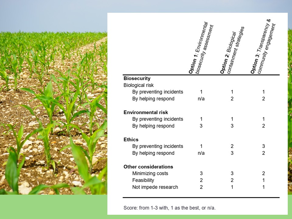
4. Comparative Evaluation

Scoring table to be inserted here.

5. Prioritization of Governance Options

Based on the updated scoring table, a combination of:

• Option 1: Environmental Biosecurity Assessment
• Option 2: Biological Containment Strategies

is prioritized.

These two options are essential for project viability because they:

• Perform best in preventing biological and environmental risks
• Address core ethical concerns
• Strengthen long-term sustainability of the project

Although they may involve:

• Higher implementation costs
• Potential constraints on research

they are necessary to ensure responsible development.

Role of Option 3

Transparency and community engagement is not critical for technical viability but is essential for:

• Implementation in agricultural plantations
• Social acceptance
• Practical adoption by farming communities

Conclusion

A combined governance strategy integrating:

• Environmental biosecurity assessment
• Technical biological containment
• Community engagement

provides a balanced framework that aligns:

• Safety
• Technical feasibility
• Ethical responsibility
• Real-world applicability

This integrated approach supports the responsible development and deployment of a bioindicator system for detecting microplastic contamination in agricultural soils.

DNA Replication, Oligo Synthesis, and Molecular Coding Concepts

Questions from Professor Jacobson

DNA Replication Fidelity

Nature’s machinery for copying DNA is DNA polymerase, which has an error rate of approximately 1 in 10⁶ bases due to its 3’→5’ proofreading activity.

The human genome contains approximately 3 × 10⁹ base pairs. In principle, thousands of errors could occur during a complete replication cycle. However, biological systems maintain genomic integrity through multiple mechanisms:

• Polymerase proofreading activity
• Exonuclease activity
• DNA repair systems

Together, these systems significantly reduce the final mutation rate and preserve genomic stability.

Combinatorial Space of Protein-Coding Sequences

There are approximately:

3^{400 ≈ 10}190

possible DNA sequences that could encode an average human protein of 400 amino acids.

In practice, many theoretical sequences are non-functional due to constraints such as:

• Codon bias
• mRNA secondary structure
• Translation efficiency
• Splicing motifs
• Protein folding constraints

Thus, while the combinatorial sequence space is vast, functional protein-coding sequences represent only a small subset.

Questions from Dr. LeProust

Most Common Method for Oligonucleotide Synthesis

The most widely used method for oligonucleotide synthesis today is solid-phase phosphoramidite chemistry (β-cyanoethyl phosphoramidite method).

It is performed on a solid support, typically:

• Controlled pore glass (CPG)
• Functionalized silica

The synthesis proceeds through iterative cycles consisting of:

1. Coupling of a protected nucleoside phosphoramidite
2. Capping of unreacted hydroxyl groups
3. Oxidation of the phosphite triester to a phosphate triester
4. DMT deprotection (deblocking)

This cycle is repeated until the desired sequence is assembled.

Why Is It Difficult to Synthesize Oligos Longer Than 200 nt?

Direct solid-phase phosphoramidite synthesis becomes inefficient beyond approximately 200 nucleotides because each nucleotide addition step is not 100% efficient (typically ~99%).

Since each step introduces a small loss, the total yield decreases exponentially with length.

Consequences include:

• Cumulative yield loss
• Exponential decrease in full-length product
• Accumulation of truncated sequences
• Increased error rates
• Increasingly difficult purification

For example, if each step is 99% efficient, after 200 cycles the overall yield is:

0.99^200

which results in a significant reduction of full-length product.

Therefore, beyond ~200 nt, direct synthesis becomes impractical.

Why Can’t a 2000 bp Gene Be Synthesized Directly?

A 2000 base pair gene cannot be synthesized by direct chemical oligo synthesis for the same reason: cumulative inefficiency.

Attempting 2000 consecutive synthesis cycles would result in:

• Negligible yield of full-length product
• Massive accumulation of truncated fragments
• Increased error rates
• Impractical purification requirements

Instead, modern approaches use high-throughput synthesis platforms (e.g., chip-based synthesis) to generate millions of short oligos (typically 60–150 nt) in parallel.

These shorter fragments are then assembled into full-length genes using methods such as:

• PCR-based assembly
• Gibson Assembly

This strategy allows efficient production of thousands of genes (e.g., 9,600 genes) in a practical and scalable way.

In summary, long genes are not synthesized directly because the chemistry is inefficient at that scale; instead, short oligos are synthesized and subsequently assembled.

Question from George Church

The 10 Essential Amino Acids in Animals

The essential amino acids (those that must be obtained from the diet) are:

• Histidine
• Isoleucine
• Leucine
• Lysine
• Methionine
• Phenylalanine
• Threonine
• Tryptophan
• Valine
• Arginine (essential in many animals, especially during growth)

Implications for the “Lysine Contingency”

Since lysine is already an essential amino acid in animals, metabolic dependence on lysine is not unusual in biology.

However, lysine is naturally present in many environments and food sources. Therefore, engineering an organism to depend on lysine as a containment strategy may offer limited biosafety, because the amino acid is neither rare nor synthetic.

This suggests that dependence on a non-natural amino acid would provide a stronger and more reliable biocontainment strategy.

Coding Relationships in Molecular Biology

AA:NA and NA:NA Codes

Definitions:

• AA = Amino Acid
• NA = Nucleic Acid (DNA or RNA)

NA:NA Code

Refers to nucleic acid–nucleic acid interactions, specifically base-pairing rules:

• A–T (or A–U in RNA)
• C–G

These interactions govern information storage and replication.

AA:NA Code

Refers to the genetic code: codons in nucleic acids specify which amino acids are incorporated into a protein.

This code determines the primary amino acid sequence of a protein.

What Code Would Describe AA:AA Interactions?

AA:AA interactions refer to amino acid–amino acid interactions within or between proteins, including:

• Hydrophobic interactions
• Hydrogen bonds
• Ionic interactions
• Disulfide bonds
• Van der Waals forces

These interactions determine:

• Protein folding
• Three-dimensional structure
• Stability
• Function

Unlike the genetic code, AA:AA interactions do not form a simple digital code. Instead, they constitute a physicochemical interaction framework that governs protein behavior.

Using the AA:NA code, we can program the amino acid sequence of a protein. By selecting specific amino acids, we indirectly influence AA:AA interactions and therefore affect structure and function.

However, although protein sequences can be designed, final folding and functionality cannot always be predicted with certainty. Protein structure emerges from complex and sometimes unpredict

Week 2 HW: DNA read, write and edit.

Part I: Benchling & In-silico Gel Art

Begin by importing your DNA sequence and use the Digests tool to test the effects of different restriction enzyme(s). Export your final design as a png and compare with your lab results on your Notion page. See the images below for where to find the Digests tool, selecting the “NEB 2-log” ladder in the Virtual Digest tab, and how to have multiple Digests appear in the same Virtual Digest.

First, I accessed the website https://rcdonovan.com/gel-art to create a sketch of a design based on the lambda sequence with the restriction enzymes:

• EcoRI-HF
• HindIII-HF
• BamHI-HF
• KpnI-HF
• EcoRV-HF
• SacI-HF
• SalI-HF

which I will perform using electrophoresis.

After experimenting a bit with the enzymes and the sequence (lamba), I decided to draw a “sunrise in a forest”.

Electrophoresis Overview

Now let’s talk about electrophoresis. We start with a lambda DNA sequence of about 48,500 base pairs, which we cut into fragments of different sizes using restriction enzymes. During electrophoresis, these DNA fragments are loaded into wells in a gel and move through the gel when an electric current is applied.

The fragments travel at different speeds depending on their size:

• Larger fragments move more slowly and cover shorter distances.
• Smaller fragments move faster and travel farther.

By observing how far each fragment migrates, we can use this pattern to create the chosen visual representation.

Benchling Simulation

Let’s go to the Benchling website (benchling.com) to perform a simulation of electrophoresis using the proposed DNA sequence and restriction enzymes.

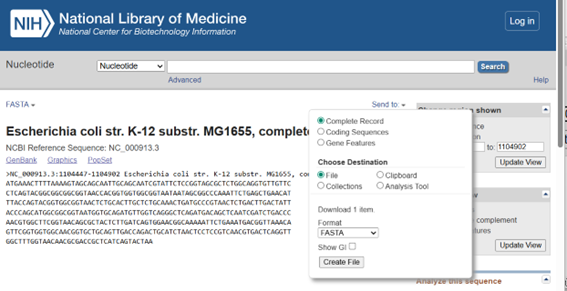
To find the GenBank accession number for the lambda sequence (#lambda sequence in GenBank) Google was used. The number for the lambda is J02459.1. Clicking on this number opens the sequence directly on the NIH website (National Library of Medicine, www.ncbi.nlm.nih.gov).

Click on FASTA, which will open a menu. Adjust the options as needed and then download the file.

Now, open https://benchling.com/ create a project and import the sequence.

Next, select the scissors icon on the right to perform a digest in the Virtual Digest tab. Choose the restriction enzyme and carry out the digestion.

The program will simulate electrophoresis for each well, showing how far the DNA fragments migrate. After performing digests for all nine wells and selecting the ladder, we will have the final proposed image.

Figure: “Sunrise in the Forest,” sun and tree in the image.

Part 2: Gel Art – Restriction digests and Gel Electrophoresis

Since I did not have access to the lab to perform this section, I will use a gel that I ran a couple of weeks ago:

To determine the fragment size, we compared it with the ladder (on the right of each row).

The fragments are approximately 6,000 bp.

The color does not determine the size. The DNA size is determined by the migration distance.

The bands are clear and well separated, indicating that the electrophoresis ran correctly. No lateral smearing or fuzzy bands are observed, which indicates good gel preparation and proper sample loading.

Part 3: DNA Design Challenge (proposal)

• Promoter

  • Name: BBa_J23106
  • Type: Constitutive promoter
  • Sequence: TTTACGGCTAGCTCAGTCCTAGGTATAGTGCTAGC
  • Purpose: Initiates transcription of PETase.

• RBS + Start codon (ATG)

  • Sequence: CATTAAAGAGGAGAAAGGTACCATG
  • Purpose: Ribosome binding and translation initiation.

• CDS (PETase codon-optimized)

  • Name: PETase_Ecoli_codopt
  • Sequence: tu secuencia codón optimizada aquí
  • Purpose: Codes for the PETase protein.

• His-tag (optional, C-terminal)

  • Sequence: CATCACCATCACCATCATCAC (7x His)
  • Purpose: Facilitates purification of PETase protein.

• Stop codon

  • Sequence: TAA
  • Purpose: Terminates translation.

• Terminator

  • Example: BBa_B0015
  • Sequence: CCAGGCATCAAATAAAACGAAAGGCTCAGTCGAAAGACTGGGCCTTTCGTTTTATCTGTTGTTTGTCGGTGAACGCTCTCTACTAGAGTCACACTGGCTCACCTTCGGGTGGGCCTTTCTGCGTTTATA
  • Purpose: Stops transcription and stabilizes mRNA.

• Antibiotic resistance / selectable marker

  • Example: Ampicillin (AmpR)
  • Purpose: Selects for bacteria that successfully took up the plasmid.

3.1. Choose your protein

PETase Protein Sequence Description

The protein used in this project is a Poly(ethylene terephthalate) hydrolase (PETase), also known as a PET-digesting enzyme. Its UniProt/NCBI accession is A0A0K8P6T7.1, and it is composed of 290 amino acids. This enzyme originates from a bacterial source and is capable of degrading PET plastic. The sequence has been selected for codon optimization to enable expression in E. coli, facilitating the construction of a plasmid-based reporter system for PET detection in environmental samples.

The PETase protein sequence was obtained from Ideonella sakaiensis by accessing the NIH protein database at https://www.ncbi.nlm.nih.gov/protein and searching for “PETase Ideonella sakaiensis.” The protein entry was selected, and the sequence was downloaded in FASTA format for subsequent use in codon optimization and plasmid design.

I downloaded the Proteine.fasta file.

I examined and visualized the features of the protein sequence through the Features option.

3.2. Reverse Translate: Protein (amino acid) sequence to DNA (nucleotide) sequence.

There are available on internet many Codon Optimization Tools (IDT, Twist, GenScript, VectorBuilder, ExoOptimizer…). I chose Vector Builder Optimization Tool (https://en.vectorbuilder.com/).

The PETase protein sequence in FASTA format was used as input in
VectorBuilder → Tools → Codon Optimization Tool.

• The amino acid sequence was pasted directly, specifying it as a protein sequence.
• The host organism was set to Escherichia coli str. K-12 substr. MG1655 to optimize codon usage for this bacterium.
• No restriction sites were selected for avoidance.

The tool generated a DNA sequence (ORF) optimized for E. coli, with the following characteristics:

• Start codon: ATG and stop codon: TAA
• GC content: 59.56%
• Codon Adaptation Index (CAI): 0.91, indicating high compatibility with E. coli codon preferences.
• The sequence is now ready to be inserted into a plasmid for expression.

3.3. Codon optimization

NOTE: Codon optimization was performed along with reverse translation in Vector Builder (VB).

Codon optimization is important because, although multiple codons can encode the same amino acid, different organisms preferentially use certain codons more frequently. If a gene contains codons that are rarely used in the host organism, translation may be inefficient, leading to low protein expression. By optimizing codon usage, I adapted the PETase nucleotide sequence to match the codon preferences of Escherichia coli without altering the amino acid sequence of the protein.

For this project, I chose to optimize PETase for E. coli because it is the host organism where the plasmid will be expressed. Since PETase originates from the bacterium Ideonella sakaiensis, its native codon usage differs from E. coli, so codon optimization improves expression efficiency in this bacterial system.

During codon optimization, restriction enzyme recognition sites were not specifically removed because the sequence was designed for direct insertion into a plasmid using VectorBuilder, which ensures proper assembly. This optimization ensures high expression of PETase in E. coli, allowing the gene to be used effectively in the plasmid as a biological marker for PET detection.

3.4. You have a sequence! Now what?

Producing PETase from the Optimized DNA Sequence

The codon-optimized DNA sequence for PETase can be expressed using cell-dependent or cell-free systems. In bacteria like E. coli, the plasmid is transcribed into mRNA and translated into protein using the host’s machinery, with selection markers ensuring only cells carrying the gene produce PETase. Alternatively, cell-free systems synthesize protein directly from the DNA in vitro, without living cells. Optimizing the sequence ensures efficient production of functional PETase for detection or degradation of PET.

Both approaches follow the central dogma of molecular biology: DNA is transcribed into RNA, and RNA is translated into protein.

3.5. How does it work in nature/biological systems?

In nature, a single gene contains the information to produce a protein through transcription and translation. The DNA sequence of the PETase gene is first transcribed into messenger RNA (mRNA) by RNA polymerase. This mRNA serves as a template for translation, where ribosomes read the codons in sets of three nucleotides to assemble the corresponding amino acids into the PETase protein.

Some genes in biological systems can produce multiple protein variants through mechanisms such as alternative splicing, alternative start codons, or frameshifting, but PETase from Ideonella sakaiensis produces a single functional protein. Aligning the DNA sequence, the transcribed RNA, and the translated protein shows how the nucleotide code directly determines the amino acid sequence of the protein.

The construct of DNA and amino acids was obtained in genscript during codon optimization sequence.

Part 4: Prepare a Twist DNA Synthesis Order

4.1. Create a Twist account and a Benchling account

Twist account doesn’t work properly. I used instead VectorBuilder and Benchling.

4.2. Build a DNA Insert Sequence

I adjusted the proposed PETase plasmid design as follows:

I have to build a DNA Insert Sequence from the Promoter to Terminator, which includes:

• Promoter – initiates transcription of the gene. (BBa_J23106 TTTACGGCTAGCTCAGTCCTAGGTATAGTGCTAGC, position 1-35).
• Ribosome Binding Site (RBS / Kozak) – ensures proper ribosome binding and efficient translation initiation (Kozak GCCACC, position 36 - 41).
• Start Codon – defines the beginning of the open reading frame (ATG, position 42 - 44).
• Codon-Optimized PETase ORF – DNA codon optimized sequence for E. coli (position 45 – 911).
• Stop Codon – properly terminates translation (TAA, position 912 - 914).
• Transcription Terminator – ensures transcription stops correctly (BBa_B0015 CCAGGCATCAAATAAAACGAAAGGCTCAGTCGAAAGACTGGGCCTTTCGTTTTATCTGTTGTTTGTCGGTGAACGCTCTCTACTAGAGTCACACTGGCTCACCTTCGGGTGGGCCTTTCTGCGTTTATA).
• Antibiotic Selection Marker – allows selection of bacteria carrying the plasmid (Ampicillin - Amp).

In Benchling, I create a new sequence that will result from sequentially adding the DNA corresponding to the proposed plasmid design. I am going to create an insert sequence manually.

Then click Sequence Map and right-clicking over the sequence and create an annotation that describes what each piece is.

This final construct ensures correct transcription and translation of the PETase protein in a bacterial expression system.

I clicked on Linear Map, to preview the sequence (https://benchling.com/s/seq-XuMlxoCIaSAHse8uxNbh?m=slm-UieHiRHS78CKGHaLm4cL).

I downloaded both files:

• PETase_Ecoli_insert.pdf

• PETase_Ecoli_insert-sequence.pdf

  

And I also exported and downloaded the FASTA file for the constructed sequence.

The final assembled sequence is known as an expression cassette, since it contains all the necessary elements required for gene expression, including the promoter, RBS, start codon, codon-optimized PETase coding sequence, stop codon, and terminator.

This cassette can be downloaded as a FASTA file for further use. In this format, the sequence can be shared, analyzed, synthesized, or inserted into a circular plasmid backbone for recombinant protein expression.

To visualize the genetic construct, I used SBOL Canvas to create a standardized graphical representation of the expression cassette. This tool allowed me to clearly illustrate the organization of the promoter, Kozak, codon-optimized PETase coding sequence, and terminator.

4.3. VectorBuilder: clonal genes

For this project, we selected the Clonal Genes option because it provides the DNA sequence cloned into a circular plasmid backbone, ready for direct transformation into E. coli.

Since the Twist Bioscience platform was not accessible, VectorBuilder was used as an alternative to insert the cassette into the plasmid backbone. VectorBuilder offers similar gene synthesis and cloning services, enabling the insertion of the designed expression cassette into a suitable plasmid backbone for bacterial expression. This alternative allows the construct to be obtained as a ready-to-use circular DNA molecule for transformation and recombinant protein production.

Open VectorBuilder and choose a vector system. I have chosen a bacterial recombinant protein expression vector (pET Guide) to express the codon-optimized PETase in E. coli. This vector is designed for high-level protein expression, supports all essential elements (RBS, start/stop codons, optional tags, terminator), and allows selection with antibiotics. It provides a reliable and compatible platform for producing functional PETase in a bacterial system.

I did not add a purification tag to PETase at this stage. The protein can be expressed and remain functional without a tag, and a His-tag or other purification tag can be added later if needed for downstream applications.

The vector was constructed using the codon-optimized DNA of the PETase protein. A PDF file (VB260217-1695xnz(pET-{PETase ORF codon_optimized_DNA}).pdf) containing the vector information, a FASTA file (VB260217-1695xnz.fasta) with the sequence, and a GenBank file (VB260217-1695xnz.gb) were downloaded.

When selecting the vector, I was presented with other options that I was not certain were appropriate. It is important to carefully evaluate which vector is most suitable and to ensure that the promoters, RBS, and other components included in the vector are optimal for this project.

Part 5: DNA Read/Write/Edit

5.1 DNA Read

1. What DNA would you want to sequence (e.g., read) and why?

I would sequence DNA from soil or ocean microbial communities exposed to plastic, aiming to detect PETase or other plastic-degrading genes. This would help identify microorganisms capable of PET degradation and monitor their presence in different environments. I would also like to work with fossil and isolated organisms to better understand evolutionary adaptations.

2. What technology or technologies would you use to perform sequencing on your DNA and why?

I would use Illumina NGS (Sequencing by Synthesis) for high-throughput and accurate sequencing of environmental DNA. For fossil or isolated organisms, long-read technologies such as PacBio or Oxford Nanopore could help assemble fragmented genomes.

3. Is your method first-, second-, or third-generation? How so?

For detecting PETase genes in environmental samples, Illumina NGS (Sequencing by Synthesis) is a second-generation sequencing method. It produces millions of short reads in parallel, offering high throughput and accuracy, which makes it ideal for complex samples.

4. What is your input? How do you prepare your input? List the essential steps.

The input for Illumina NGS is extracted DNA from environmental samples. Essential steps include: DNA extraction, fragmentation, adapter ligation, PCR amplification, and library quality control before sequencing.

5. What are the essential steps of your chosen sequencing technology? How does it decode the bases of your DNA sample (base calling)?

Illumina Sequencing by Synthesis works by attaching DNA fragments to a flow cell and amplifying them into clusters. Fluorescently labeled nucleotides are incorporated one at a time, and after each incorporation, imaging captures the fluorescent signal. Software then converts these signals into base calls (A, C, G, T).

6. What is the output of your chosen sequencing technology?

The output of Illumina sequencing consists of FASTQ files containing DNA sequences and quality scores for each base. If multiple samples are sequenced together, the reads are demultiplexed using sample-specific barcodes.

5.2 DNA Write

1. What DNA would you want to synthesize and why?

I would like to synthesize genes related to environmental rescue, including biosensors, plastic-degrading enzymes such as PETase, and biomaterials for bioremediation. These DNA constructs could allow microorganisms to detect pollutants, respond to environmental stimuli, and break down plastics. For example, I would include the codon-optimized PETase ORF used in this project, along with regulatory elements such as promoters and ribosome binding sites to ensure proper expression.

2. What technology or technologies would you use to perform this DNA synthesis and why?

I would use commercial DNA synthesis platforms such as Twist Bioscience or enzymatic DNA synthesis methods. These technologies allow accurate and customizable synthesis of codon-optimized genes and regulatory elements. They are scalable, precise, and suitable for constructing complete expression cassettes.

3. What are the essential steps of your chosen DNA synthesis method?

DNA synthesis typically involves chemically or enzymatically synthesizing short oligonucleotides, assembling them into longer DNA fragments, verifying sequence accuracy, and cloning the construct into a plasmid backbone. The final product is then amplified and quality-checked before delivery.

4. What are the limitations of your DNA synthesis method in terms of speed, accuracy, and scalability?

DNA synthesis can be limited by cost, turnaround time, and potential synthesis errors in long or repetitive sequences. Very large constructs may require hierarchical assembly, increasing complexity and time.

5.3 DNA Edit

1. What DNA would you want to edit and why?

I would like to edit genes in microorganisms involved in plastic degradation to improve their efficiency, stability, or environmental tolerance. For example, I could modify the PETase gene to enhance its catalytic activity or thermal stability. Editing could also be applied to environmental bacteria to optimize metabolic pathways for bioremediation.

2. What technology or technologies would you use to perform these DNA edits and why?

I would use CRISPR-Cas systems because they provide precise, efficient, and versatile genome editing capabilities in microorganisms, plants, or animals.

3. How does your technology of choice edit DNA? What are the essential steps?

CRISPR-Cas uses a guide RNA designed to match a specific DNA target sequence. The Cas nuclease creates a double-strand break at the target site. The cell then repairs the break either through non-homologous end joining (causing insertions or deletions) or homology-directed repair (allowing precise edits if a repair template is provided).

4. What are the limitations of your editing method in terms of efficiency or precision?

CRISPR-Cas systems may have off-target effects, variable editing efficiency depending on the target sequence, and limitations related to delivery methods. Additionally, precise edits require efficient homology-directed repair, which may not occur at high frequency in all cell types.

Week 03 HW: Lab Automation

WEEK 3 — LAB AUTOMATION

LAB PROTOCOL

1. Review of Materials

First, I reviewed the available documentation on HTGAA (LAB–Week 3 – Opentrons Art). Key information required to prepare the design was found at the beginning of the Google Colab notebook, including technical constraints and recommended parameters for droplet spacing and volume.

2. Design Generation

I generated the artistic design using the GUI available at:
https://opentrons-art.rcdonovan.com

Initially, I had questions regarding droplet size and spacing between points. The Google Colab notebook provided specific recommendations about these parameters.

Before identifying these constraints, I created a version of the design with reduced spacing between points to increase visual detail. However, decreasing the distance between droplets increased the risk of unintended merging during robotic dispensing. After reviewing the guidelines, I adjusted the design to comply with the recommended 3.5 mm spacing.

From Donovan’s platform, I downloaded the coordinate sets to be used in the Python script. The coordinates were grouped by color and already respected the recommended spacing (3.5 mm).

The design was registered on the platform under the following ID:
https://opentrons-art.rcdonovan.com/?id=w8392ofgw0pexpu

_{Figure Art design}

3. Script Development and Simulation

I opened the HTGAA26 Opentrons Colab notebook and created a personal copy to develop the script. The notebook included reference examples from previous students, which were useful to understand how coordinate-based dispensing is implemented on agar plates.

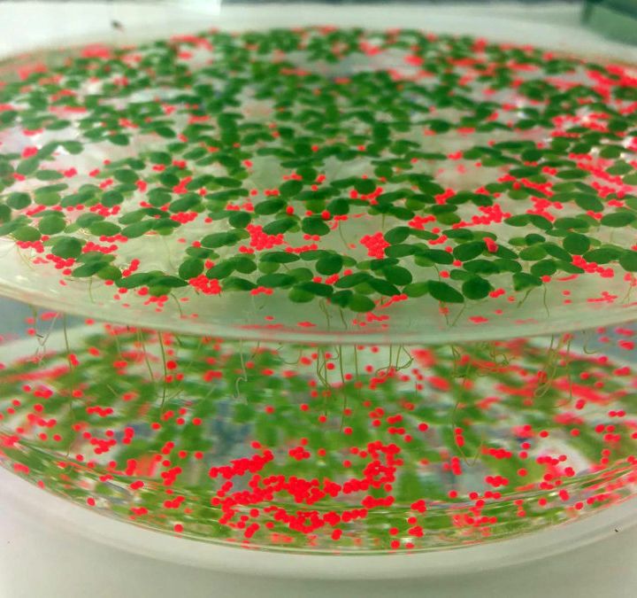
The script was written in Python. Since the laboratory setup provides only two available colors for execution, I adapted the original design as follows:

• Blue droplets were replaced with green droplets using a higher volume (1.2 µL) to create visual differentiation.
• Green and red droplets were dispensed using the recommended volume (1 µL).

After completing the implementation, I executed the simulation within the Opentrons environment. The simulation ran successfully without errors, confirming correct tip usage, aspiration logic, and coordinate positioning.

_{Figure Art design}

Here, the script:

from opentrons import types

metadata = {    # see https://docs.opentrons.com/v2/tutorial.html#tutorial-metadata
    'author': 'María José Pérez Crespo',
    'protocolName': 'Peacock',
    'description': 'Print peacock using two colors: green 1 µL, green 1.2 µL, red 1 µL',
    'source': 'HTGAA 2026 Opentrons Lab',
    'apiLevel': '2.20'
}

##############################################################################
###   Robot deck setup constants - don't change these
##############################################################################

TIP_RACK_DECK_SLOT = 9
COLORS_DECK_SLOT = 6
AGAR_DECK_SLOT = 5
PIPETTE_STARTING_TIP_WELL = 'A1'

well_colors = {
    'A1' : 'Red',
    'B1' : 'Green',
    'C1' : 'Orange'
}


def run(protocol):

  ##############################################################################
  ###   Load labware, modules and pipettes
  ##############################################################################

  tips_20ul = protocol.load_labware(
      'opentrons_96_tiprack_20ul',
      TIP_RACK_DECK_SLOT,
      'Opentrons 20uL Tips'
  )

  pipette_20ul = protocol.load_instrument(
      "p20_single_gen2",
      "right",
      [tips_20ul]
  )

  temperature_module = protocol.load_module(
      'temperature module gen2',
      COLORS_DECK_SLOT
  )

  temperature_plate = temperature_module.load_labware(
      'opentrons_96_aluminumblock_generic_pcr_strip_200ul',
      'Cold Plate'
  )

  color_plate = temperature_plate

  agar_plate = protocol.load_labware(
      'htgaa_agar_plate',
      AGAR_DECK_SLOT,
      'Agar Plate'
  )

  center_location = agar_plate['A1'].top()

  pipette_20ul.starting_tip = tips_20ul.well(PIPETTE_STARTING_TIP_WELL)

  ##############################################################################
  ###   Helper functions
  ##############################################################################

  def location_of_color(color_string):
      for well, color in well_colors.items():
          if color.lower() == color_string.lower():
              return color_plate[well]
      raise ValueError(f"No well found with color {color_string}")


  def dispense_and_detach(pipette, volume, location):
      assert isinstance(volume, (int, float))
      above_location = location.move(types.Point(z=location.point.z + 5))
      pipette.move_to(above_location)
      pipette.dispense(volume, location)
      pipette.move_to(above_location)


  ##############################################################################
  ###   Definición de puntos
  ##############################################################################

  sfgfp_points = [...]
  mrfp1_points = [...]
  electra2_points = [...]

  ##############################################################################
  ###   Centrado automático
  ##############################################################################

  all_points = sfgfp_points + mrfp1_points + electra2_points

  min_x = min(pt[0] for pt in all_points)
  max_x = max(pt[0] for pt in all_points)
  min_y = min(pt[1] for pt in all_points)
  max_y = max(pt[1] for pt in all_points)

  offset_x = (min_x + max_x) / 2
  offset_y = (min_y + max_y) / 2


  ##############################################################################
  ###   Green (new tip)
  ##############################################################################

  green_loc = location_of_color('Green')
  pipette_20ul.pick_up_tip()

  remaining_total_volume = len(sfgfp_points) * 1.0 + len(electra2_points) * 1.2
  current_volume = 0.0

  for point in sfgfp_points:
      vol = 1.0
      if current_volume < vol:
          load_volume = min(20, remaining_total_volume)
          pipette_20ul.aspirate(load_volume, green_loc)
          current_volume += load_volume

      x_mm, y_mm = point
      target_location = center_location.move(
          types.Point(x=x_mm - offset_x, y=y_mm - offset_y, z=0)
      )

      dispense_and_detach(pipette_20ul, vol, target_location)

      current_volume -= vol
      remaining_total_volume -= vol


  for point in electra2_points:
      vol = 1.2
      if current_volume < vol:
          load_volume = min(20, remaining_total_volume)
          pipette_20ul.aspirate(load_volume, green_loc)
          current_volume += load_volume

      x_mm, y_mm = point
      target_location = center_location.move(
          types.Point(x=x_mm - offset_x, y=y_mm - offset_y, z=0)
      )

      dispense_and_detach(pipette_20ul, vol, target_location)

      current_volume -= vol
      remaining_total_volume -= vol


  pipette_20ul.drop_tip()


  ##############################################################################
  ###   RED color (New tip)
  ##############################################################################

  red_loc = location_of_color('Red')
  pipette_20ul.pick_up_tip()

  remaining_total_volume = len(mrfp1_points) * 1.0
  current_volume = 0.0

  for point in mrfp1_points:
      vol = 1.0
      if current_volume < vol:
          load_volume = min(20, remaining_total_volume)
          pipette_20ul.aspirate(load_volume, red_loc)
          current_volume += load_volume

      x_mm, y_mm = point
      target_location = center_location.move(
          types.Point(x=x_mm - offset_x, y=y_mm - offset_y, z=0)
      )

      dispense_and_detach(pipette_20ul, vol, target_location)

      current_volume -= vol
      remaining_total_volume -= vol


  pipette_20ul.drop_tip()

4. Use of AI Assistance

Artificial intelligence tools were used to support the development of the script. The structural logic was based on the provided examples in the notebook, particularly Example 7 (Microbial Earth), which clarified how grouped coordinates are iterated and dispensed.

AI assistance was used to:

• Understand how the center of the agar plate is calculated.
• Implement coordinate offset correction for centering the design.
• Structure iteration over grouped coordinate lists while maintaining color consistency.
• Optimize aspiration logic to minimize reagent waste.

The questions posed were specific and focused on resolving implementation details. AI was used as a technical support tool rather than as a replacement for understanding the protocol logic.

5. Robot Scheduling

I already booked Friday 27, 14.00

6. Submission

The Python script was submitted via the corresponding Google Form, and confirmation was received.

The script was shared using the following link:

https://colab.research.google.com/drive/15lHDPfQqFryL9ydvX3P-SeppB7QAd0d8?usp=sharing

Additionally, the metadata section generated the following direct cell link:

https://colab.research.google.com/drive/15lHDPfQqFryL9ydvX3P-SeppB7QAd0d8#scrollTo=t5Bt7VmS_JF_&line=17&uniqifier=1

POST LAB QUESTIONS

1. Find and describe a published paper that utilizes the Opentrons or an automation tool to achieve novel biological applications.**

Rosini, E., Battaglia, C., Miani, D., Molinari, F., Arrigoni, F., Piarulli, U., … & Pollegioni, L. (2025). Valuable compounds from pollutants: converting PET into enantiopure alanine. ACS Catalysis, 15(21), 17829-17843.

In this study, the Opentrons OT‑2 automated pipetting system was used to perform a colorimetric assay with PSP dye, which allows measurement of pH changes associated with terephthalic acid (TPA) production during PET depolymerization. The automation enabled rapid and consistent processing of multiple samples, improving the reproducibility and efficiency of depolymerizing enzyme screening. The Opentrons OT‑2 automated system was used to perform a PSP colorimetric assay to measure pH changes during PET depolymerization, enabling fast and reproducible enzyme screening.

2. Write a description about what you intend to do with automation tools for your final project. You may include example pseudocode, Python scripts, 3D printed holders, a plan for how to use Ginkgo Nebula, and more. You may reference this week’s recitation slide deck for lab automation details.**

No ideas already.

FINAL PROJECT IDEAS

No ideas already.

Week 4 HW: Protein Design - Part I

Part A. Conceptual Questions

How many molecules of amino acids do you take with a piece of 500 grams of meat?

First, I researched how much protein the meat contains. I assumed it was beef, and I saw that the amount of protein per gram varies depending on the cut (FEN, 2012). I calculated the average protein content of 10 cuts and got 19.46, which I rounded up to 20g per 100g.

• A Dalton is a unit of molecular mass defined as 1 atomic mass unit (amu) which is 1/12 of the mass of a carbon 12 atom.
  1 Da ~ mass of a single proton or neutron ~ 1.66 x 10-24 g
  100 Da ~ 1.66 x 10-22 g/molecule, that is the mass of a single amino acid (one molecule).
• g of Protein to moles of amino acids:
  Moles of amino acids = (mass of protein (g)) / (average molecular weight per amino acid (g/mol))
  (100 g)/(100 g/mol) = 1 mol of amino acid
• If (Avogadro’s number): 1 mol = 6.022 x 10²³ molecules/mol

How many molecules in 1 mol of amino acids? ~6.022 x 10²³ molecules/mol in 500 gr of meat

Why do humans eat beef but do not become a cow, eat fish but do not become fish?

Because humans eat food that provides molecules, not organisms.

Why are there only 20 natural amino acids?

The 20 amino acids were selected based on availability, stability, and functional suitability, forming an optimal set for building proteins in early life.

There are only 20 standard amino acids because evolution selected a set that is chemically diverse, structurally compatible with protein folding, and efficient for accurate translation.

While more amino acids were likely available early on, translation precision and the need to reduce errors led to the retention of this specific set (Weber & Miller, 1981).

Can you make other non-natural amino acids? Design some new amino acids.

Non-natural amino acids can be designed to introduce new functions, enhance stability, or modify reactivity in proteins, extending the capabilities of the 20 standard amino acids; however, their exact behavior cannot be fully predicted, so careful experimental validation and optimization are essential.

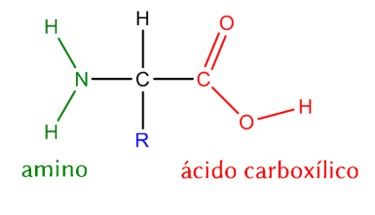
To design a new amino acid, I need to study their structure, variability, and functionality:

Structure and Function of α-Amino Acids

• Central α-carbon – the connection point for all groups.
• Amino group (-NH₂) – basic, participates in peptide bonds.
• Carboxyl group (-COOH) – acidic, participates in peptide bonds and proton transfer.
• Hydrogen (H) – small, allows proper folding.
• Side chain (R group) – variable, determines the chemical properties and identity of the amino acid.

Variability:

Differences between amino acids come from the R group, which can be hydrophobic, polar, acidic, basic, aromatic, or special (like cysteine or proline).

Functional roles:

Amino and carboxyl groups: form the peptide backbone and participate in chemical reactions.
Side chain (R): defines polarity, charge, reactivity, hydrogen bonding, and overall protein structure.

Design implications:

Synthetic amino acids often modify the side chain (R) to introduce new chemical functions, stability, or reactivity.
Modifying the α-carbon, amino, or carboxyl groups is less common but can create β-amino acids or N-alkylated variants, affecting folding.

The side chain (R group) determines the identity and functionality of an amino acid, while the backbone maintains the ability to form proteins. Synthetic modifications expand the chemical possibilities beyond the 20 standard amino acids.

Now, I do not know much about synthetic modifications, and I asked chatgpt3:

I also found an interesting article about synthetic amino acids (Rovner et al., 2015), it shows a practical application of synthetic amino acids (sAAs) to control and engineer organisms, and expand protein functionality beyond natural amino acids:

• Incorporation into essential proteins: TAG codons in key genes are reassigned to encode synthetic amino acids, demonstrating how sAAs can be integrated into functional proteins.
• Biocontainment: Cells only grow when supplied with sAAs, highlighting their use for controlling viability.
• Expanding the genetic code: sAAs enable new chemical functionalities beyond the 20 natural amino acids, allowing the design of synthetic proteins with novel properties.

Where did amino acids come from before enzymes that make them, and before life started?

Before enzymes and living cells existed, amino acids likely formed through natural (abiotic) chemical processes. The main explanations are:

• Chemical reactions on early times of earth: On the early Earth, simple atmospheric gases such as carbon dioxide (CO₂), methane (CH₄), ammonia (NH₃), and hydrogen (H₂) are thought to have reacted under energy sources such as lightning, volcanic heat, and ultraviolet radiation. Within the theoretical framework proposed by Alexander Oparin (1924, 1938) and J. B. S. Haldane (1929), these energy-driven processes could have led to the abiotic formation of organic molecules in the primitive oceans. Experimental support for this hypothesis was later provided by the Miller-Urey experiment (Miller, 1953), which demonstrated that amino acids can form under simulated early Earth conditions.
• Formation in space and delivery to Earth: Amino acids may also have formed in space and later been delivered to Earth through cometary and asteroidal material. Organic compounds, including amino acids and phosphorus-bearing molecules, have been detected in the coma of comet 67P/Churyumov-Gerasimenko, demonstrating that prebiotic chemicals can form in extraterrestrial environments (Altwegg et al., 2016). More recently, samples from the asteroid Bennu returned by NASA’s OSIRIS-REx revealed amino acids whose isotopic signatures suggest formation in very cold primordial ices in the early Solar System (Baczynski et al 2026).
• Mineral catalysis before enzymes: Mineral surfaces and metal ions on the early Earth could have acted as simple catalysts before enzymes evolved, helping to concentrate organic compounds and promote chemical reactions. Recent reviews show that clays and other minerals can adsorb and organize amino acids and other prebiotic molecules, enhancing their reactions and potentially aiding the formation of more complex organics such as peptides and polymers in prebiotic settings (Nogal et al., 2023).

Overall, evidence suggests that amino acids existed before life began, and enzymes evolved later to make these natural chemical processes more efficient.

If you make an α-helix using D-amino acids, what handedness (right or left) would you expect?

If an α-helix is constructed entirely from D-amino acids, the helix will adopt the opposite handedness compared to a helix made of L-amino acids and its functionality can change. Natural proteins are composed of L-amino acids, which form right-handed α-helices. D-amino acids are mirror images of L-amino acids, so when used exclusively, they form left-handed α-helices.

If an α-helix composed of L-amino acids is instead made entirely from D-amino acids, the helix becomes a mirror image of the original. L-amino acids form right-handed helices, while D-amino acids form left-handed helices, flipping the spatial arrangement of the side chains. Because many biological interactions are chiral-specific, this mirror-image helix often cannot interact with the same enzymes, receptors, or partners as the L-helix. As a result, the functionality can change: D-amino acid helices may be more resistant to proteases, more stable, or have novel chemical properties, but they rarely replicate the exact biological activity of the original L-amino acid helix.

Can you discover additional helices in proteins?

Yes. Additional helices in proteins can be discovered through experimental methods such as X-ray crystallography, NMR, or cryo-EM, as well as through computational structure prediction tools like AlphaFold. In some cases, regions that appear disordered can form helices only under certain conditions (for example, upon binding to another molecule), revealing previously unrecognized helical structures.

Why are most molecular helices right-handed?

Most molecular helices are right-handed because biological molecules are chiral. Proteins are built from L-amino acids, whose geometry makes the right-handed α-helix energetically more stable and free of steric clashes than the left-handed version. Similarly, the stereochemistry of sugars in DNA favors a right-handed double helix (B-DNA).

Why do β-sheets tend to aggregate?

β-sheets tend to aggregate because their structure allows strong interactions between different protein molecules.

When a protein is partially unfolded, its backbone and hydrophobic regions become exposed. β-strands from different molecules can then align side by side and form many hydrogen bonds. Their flat and extended shape also allows close packing (antiparallel, parallel, mixed).

These interactions lower the overall free energy of the system, making the aggregated β-sheet structure (such as amyloid fibrils) more stable than the unfolded proteins (Maury 2015).

Protein aggregation does not mean the native protein becomes more stable. Instead, when a protein is partially unfolded or misfolded, it is in a relatively unstable, high-energy state. Exposed hydrophobic regions and backbone groups can then form intermolecular interactions (hydrophobic contacts and hydrogen bonds, often arranged as β-sheets).

These interactions lower the overall free energy of the system, making the aggregated state more thermodynamically stable than the unfolded monomers — even though it is not the functional native state.

So, aggregation is energetically favorable compared to the misfolded/unfolded state, but it represents a loss of normal protein function.

In short, β-sheets are fundamental structural elements of proteins that are crucial for both normal function and, in some cases, disease.

What is the driving force for β-sheet aggregation?

The main driving force for β-sheet aggregation is the formation of extensive intermolecular hydrogen bonds combined with hydrophobic interactions, which lower the free energy of the system and stabilize the cross-β fibril structure.

Why do many amyloid diseases form β-sheets?

Many amyloid diseases form β-sheets because misfolded proteins can easily reorganize into this structure.

An amyloid disease is a disorder in which certain proteins misfold and form abnormal aggregates called amyloid fibrils. The proteins misfold, and form structures rich in β-sheets, sticking together and building stable fibrils. These fibrils accumulate in tissues or organs and interfere with normal cell function. Over time, this accumulation can damage cells and lead to disease (Alzheimer’s disease - amyloid-β plaques in the brain; Parkinson’s disease - α-synuclein aggregates, Systemic amyloidosis - amyloid deposits in organs like the heart or kidneys (Monsellier & Chiti 2007, Cheng et al 2012, Bolshette et al 2014).

In simple terms, an amyloid disease happens when misfolded proteins aggregate and build up in the body, causing tissue damage.

Can you use amyloid β-sheets as materials?

Yes. Amyloid β-sheets can be used as materials because their structure forms highly ordered and stable fibrils. These fibrils are strong, resistant to heat and chemical degradation, and can self-assemble into nanofibers. Because of these properties, researchers are exploring their use in nanotechnology, tissue engineering scaffolds, biosensors, and drug delivery systems. Despite their association with disease in the body, amyloid β-sheets from vegetable protein have promising applications as engineered biomaterials. They have been applied in renewable and biodegradable bioplastics and in water purification membranes for heavy metal removal (Li et al 2023).

References

• Altwegg, K., Balsiger, H., Bar-Nun, A., et al. (2016). Prebiotic chemicals—amino acid and phosphorus—in the coma of comet 67P/Churyumov-Gerasimenko. Science Advances, 2(5), e1600285.
• Blachier, F. (2025). Amino Acids Before Life and in the First Living Organisms. In: The Evolutionary Journey of Amino Acids. Springer, Cham.
• Bolshette, N. B., Thakur, K. K., Bidkar, A. P., et al. (2014). Protein folding and misfolding in the neurodegenerative disorders: a review. Revue Neurologique, 170(3), 151-161.
• Cheng, P. N., Liu, C., Zhao, M., Eisenberg, D., & Nowick, J. S. (2012). Amyloid β-sheet mimics that antagonize protein aggregation and reduce amyloid toxicity. Nature Chemistry, 4(11), 927-933.
• Fundación Española de la Nutrición (FEN). (2012). Guía Nutricional de la Carne.
• Haldane, J. B. S. (1929). Origin of life. Ration. Annu., 148, 3–10.
• Li, T., Zhou, J., Peydayesh, M., et al. (2023). Plant protein amyloid fibrils for multifunctional sustainable materials. Advanced Sustainable Systems, 7(4), 2200414.
• Maury, C. P. J. (2015). Primordial genetics: Information transfer in a pre-RNA world based on self-replicating beta-sheet amyloid conformers. Journal of Theoretical Biology, 382, 292-297.
• Miller, S. L. (1953). A production of amino acids under possible primitive earth conditions. Science, 117(3046), 528-529.
• Monsellier, E., & Chiti, F. (2007). Prevention of amyloid-like aggregation as a driving force of protein evolution. EMBO Reports, 8(8), 737.
• Nogal, N., Sanz-Sánchez, M., Vela-Gallego, S., et al. (2023). The protometabolic nature of prebiotic chemistry. Chemical Society Reviews, 52(21), 7359-7388.
• Rovner, A. J., Haimovich, A. D., Katz, S. R., et al. (2015). Recoded organisms engineered to depend on synthetic amino acids. Nature, 518(7537), 89-93.
• Weber, A. L., & Miller, S. L. (1981). Reasons for the occurrence of the twenty coded protein amino acids. Journal of Molecular Evolution, 17(5), 273-284.

Part B. Proteine Analysis and Visualization

In this part of the homework, you will be using online resources and 3D visualization software to answer questions about proteins. Pick any protein (from any organism) of your interest that has a 3D structure and answer the following questions:

1. Briefly describe the protein you selected and why you selected it.

PETase (Poly(ethylene terephthalate) hydrolase, sp|A0A0K8P6T7.1|PETH_PISS1) is a bacterial enzyme specialized in degrading PET (polyethylene terephthalate), a polymer widely used in plastic bottles and packaging. This protein belongs to the α/β-hydrolase fold family, which includes enzymes such as lipases, esterases, and cutinases, sharing a characteristic structural fold of alternating α-helices and β-sheets, as well as a conserved catalytic triad (Ser–His–Asp/Glu) essential for its hydrolytic activity. PETase functions by breaking the ester bonds in PET, facilitating plastic biodegradation and making it a biotechnologically relevant model for enzymatic recycling studies.

This protein was selected for the molecular analysis and visualization section because its structure is well-characterized and its function is clear and measurable. It allows the application of bioinformatics tools to explore features such as folds, active sites, hydrophobic regions, and interaction patterns, demonstrating in a practical way how an enzyme’s structure is directly linked to its biological function and industrial applications.

2. Identify the amino acid sequence of your protein.

This is the amino acid sequence of the protein PETase.

• How long is it? What is the most frequent amino acid? You can use this Colab notebook to count the frequency of amino acids.

  The lenght of the proteine is 290 aminoacids, and the most common amino acid is S (Serine).

• How many protein sequence homologs are there for your protein? Hint: Use Uniprot’s BLAST tool to search for homologs.

– How to use BLAST Analysis of PETase BLAST (Basic Local Alignment Search Tool) is a program that compares a query sequence, either DNA or protein, against sequences in public databases. It is used to identify similar or homologous sequences, predict the family or likely function of a protein, and analyze evolutionary conservation or important functional motifs. For protein sequences, the BLASTp algorithm is typically used to compare amino acid sequences.

• **Step 1: Input Sequence: Copy the amino acid sequence of the protein you wish to analyze (for example, PETase from UniProt). Paste it into the “Enter Query Sequence” field. The sequence can be provided in FASTA format or as a plain amino acid string.

• PETase_A0A0K8P6T7 MNFPRASRLMQAAVLGGLMAVSAAATAQTNPYARGPNPTAASLEASAGPFTVRSFTVSRPSGYGAGTVYY…

• **Step 2: Select Target Database: I used UniProtKB/Swiss-prot, the Best for reliable and curated results. Then check the rest of parameters:

Pres Run BLAST and wait until they notify your results are ready.

File .tsv was downloaded, and also I downloaded .png file.

How to interpret the results from Blast?

The BLAST analysis against UniProtKB returned 250 highly significant hits (E-value < 10⁻⁸²).
Most sequences exhibit 47–52% identity, with some closely related homologs reaching 83–100% identity.

The identified proteins have an average length of 280–320 amino acids, which is consistent with enzymes belonging to the α/β hydrolase fold superfamily.

Functionally, the main homologs correspond to cutinases, lipases, and PET hydrolases, many of which are found in bacteria within the phylum Actinobacteria.

The presence of reviewed Swiss-Prot entries and homologs with available three-dimensional structures further supports the functional prediction.

Overall, the results indicate that the analyzed protein belongs to the α/β hydrolase superfamily and likely exhibits hydrolase activity toward ester bonds, with potential capability for polyester degradation such as PET.

3. Identify the structure page of your protein in RCSB

• When was the structure solved? Is it a good quality structure? Good quality structure is the one with good resolution. Smaller the better (Resolution: 2.70 Å)

  

The crystal structure of poly(ethylene terephthalate) hydrolase (PETase) from Piscinibacter sakaiensis corresponds to PDB entry 5XH3. The structure was published in 2018 in Proceedings of the National Academy of Sciences and determined using X-ray diffraction.
The reported resolution is 0.92 Å, indicating exceptionally high structural quality. Since lower resolution values reflect greater atomic precision, this structure provides near-atomic detail and is considered extremely reliable.
The analyzed chain (Chain A) shows 100% sequence identity with the query sequence across residues 1–290, confirming that this structure corresponds exactly to the studied protein.
In addition to the protein chain, the structure contains water molecules and other crystallographic components typical of high-resolution X-ray structures.
According to SCOP structural classification, the protein belongs to the alpha and beta (α/β) protein class, consistent with the α/β-hydrolase fold family identified through sequence analysis and BLAST results.

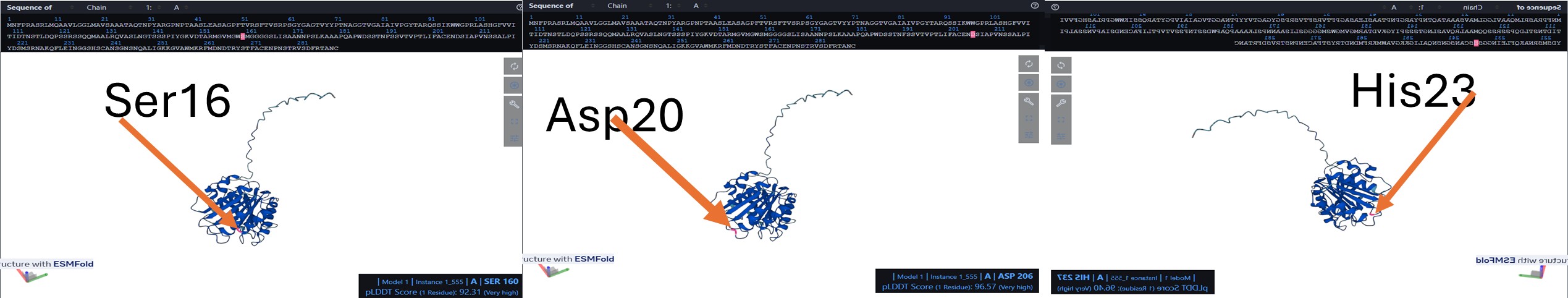
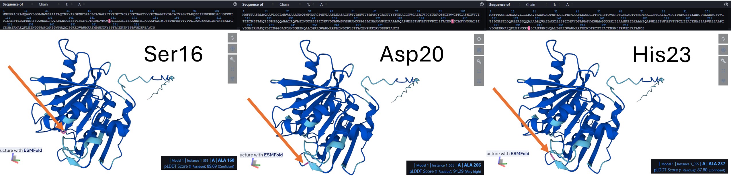
In the amino acid sequence, the catalytic triad was identified at positions Ser160, Asp206, and His237. These conserved residues form the active site of the enzyme and are responsible for its hydrolytic activity. Ser160 acts as the nucleophile, His237 functions as a general base, and Asp206 stabilizes the histidine residue. Together, this catalytic machinery enables the hydrolysis of ester bonds, consistent with the characteristic mechanism of α/β-hydrolase fold enzymes such as PETase.

See 6EQE in the picture below:

As example, Position Asp 206 (S):

• Are there any other molecules in the solved structure apart from protein?
  Yes, the crystal structure includes additional molecules such as water and crystallization agents. These are not part of the protein itself but are present due to the experimental conditions and may contribute to structural stabilization.
  The figure below (RCSB) shows other molecules such as Polymer (solid dark blue), Water (doots lighter blue around), Ion (dark blue dots) and clashes (yellow structures with pink rings).

  

• Does your protein belong to any structure classification family?
  Yes, the protein belongs to the α/β-hydrolase fold structural family, characterized by a central β-sheet surrounded by α-helices and a conserved Ser–Asp–His catalytic triad (explanation above).

4. Open the structure of your protein in any 3D molecule visualization software

• PyMol Tutorial Here (hint: ChatGPT is good at PyMol commands)
• Visualize the protein as “cartoon”, “ribbon” and “ball and stick”.

Figure description (Cartoon representation): The protein structure is shown in cartoon representation, which highlights the secondary structure elements. Red regions correspond to α-helices, yellow regions indicate β-sheets, and green regions represent loops or turns connecting the secondary structure elements. This visualization allows us to quickly see the overall fold of the protein and the organization of helices, sheets, and loops within the 3D structure.

The protein is shown in ribbon representation, highlighting its secondary structure. α-helices are colored red, β-sheets yellow, and loops/turns green. This view emphasizes the overall fold and connectivity of the protein backbone, even though short β-strands may appear as simple lines rather than arrows.

Ball-and-Stick Representation: The protein is visualized using the ball-and-stick model, where atoms are represented as spheres and bonds as sticks. The spheres are scaled to clearly show individual atoms without cluttering the image. In this representation, the distribution of atoms along the protein backbone and side chains is visible, highlighting the chemical connectivity within the enzyme. The colors correspond to residue types: for example, carbon atoms in green, oxygen in red, nitrogen in blue, and sulfur in yellow, allowing differentiation of polar, nonpolar, and reactive groups. This view emphasizes the three-dimensional arrangement of amino acids, which is critical for understanding active sites, substrate binding, and potential catalytic interactions.

• Color the protein by secondary structure. Does it have more helices or sheets?
  The protein is colored by secondary structure: red for α-helices, yellow for β-sheets, and green for loops/turns. Visually, the PETase structure contains more α-helices than β-sheets, indicating that helical regions dominate the fold, while sheets are present but less abundant. Loops and turns (green) connect these elements and form the flexible parts of the protein.

• Color the protein by residue type. What can you tell about the distribution of hydrophobic vs hydrophilic residues?
  The protein is visualized in cartoon representation, with residues colored according to their chemical properties. Hydrophobic residues (Ala, Val, Leu, Ile, Met, Phe, Trp, Tyr) are shown in orange, hydrophilic residues (Asp, Glu, Lys, Arg, His, Ser, Thr, Asn, Gln) are in cyan, and other residues such as Pro and Gly are colored gray. The distribution shows that hydrophobic residues are mostly buried within the protein core, stabilizing the structure, while hydrophilic residues are more exposed on the surface, potentially interacting with the solvent or other molecules.

• Visualize the surface of the protein. Does it have any “holes” (aka binding pockets)?
  The protein is displayed as a semi-transparent surface on a black background, highlighting the overall shape and potential binding pockets. The catalytic triad is distinctly colored: serine 160 in magenta, aspartate 206 in cyan, and histidine 237 in yellow. The triad is clearly visible on the surface, within a main binding pocket. This coloring emphasizes the spatial arrangement of the catalytic residues relative to the protein fold, allowing easy identification of the active site and nearby substrate-binding regions.

As the protein PETase belongs to the PETase / PET-digesting enzyme family, which includes hydrolases capable of degrading poly(ethylene terephthalate) (EC 3.1.1.101). This family information will be used to restrict the BLAST search to proteins with the same functional classification, ensuring that the results are relevant homologs. In Restrict by Taxonomy field, I included “bacteria”. This configuration will focus the results on relevant, functional homologs in bacterial species.

Protein AI Modeling and Analysis

In this section, we will learn about the capabilities of modern protein AI models and test some of them in your chosen protein.

a. Copy the HTGAA_ProteinDesign2026.ipynb notebook and set up a Colab instance with GPU.

b. Choose your favorite protein from the PDB.

sp|A0A0K8P6T7.1|PETH_PISS1 RecName: Full=Poly(ethylene terephthalate) hydrolase; Short=PET hydrolase; Short=PETase; AltName: Full=PET-digesting enzyme; Flags: Precursor
Sequence:
MNFPRASRLMQAAVLGGLMAVSAAATAQTNPYARGPNPTAASLEASAGPFTVRSFTVSRPSGYGAGTVYYPTNAGGTVGAIAIVPGYTARQSSIKWWGPRLASHGFVVITIDTNSTLDQPSSRSSQQMAALRQVASLNGTSSSPIYGKVDTARMGVMGWAMGGGGSLISAANNPSLKAAAPQAPWDSSTNFSSVTVPTLIFACENDSIAPVNSSALPIYDSMSRNAKQFLEINGGSASCANSGNSNQALIGKKGVAWMKRFMDNDTRYSTFACENPNSTRVSDFRTANCS

c.We will now try multiple things in the three sections below; report each of these results in your homework writeup on your HTGAA website:

C1. Protein Language Modeling

1. Deep Mutational Scans

a) Use ESM2 to generate an unsupervised deep mutational scan of your protein based on language model likelihoods.

Model Scores | Mutation Scan Heatmap | Position in Protein Sequence | Amino Acid Mutations:
The heatmap represents the log-likelihood ratio (LLR) between a mutant residue and the original amino acid (wild type, WT). Positive or less negative values indicate that a mutation is relatively tolerated by the model, whereas strongly negative values suggest that the substitution is unlikely and potentially deleterious.

b)Can you explain any particular pattern?

To answer this section, the script was improved to get visual data to support the explanation:

To investigate the mutational tolerance of the protein sequence, an unsupervised deep mutational scan (DMS) was generated using the ESM2 protein language model. In this analysis, every position of the sequence is systematically mutated to each of the 20 standard amino acids, and the model estimates the likelihood of each substitution based on learned evolutionary patterns from large protein databases.

Overall, positions 11 to 30 show that more than half of the amino acids have negative probabilities, indicating these sites are less tolerant to substitutions and likely structurally or functionally constrained. In contrast, positions 262 to 289 display predominantly positive probabilities, suggesting these regions are more flexible and can accommodate a wider range of amino acid changes without compromising stability or function. This pattern highlights differential mutational tolerance across the protein sequence.

In the figure, red markers indicate the wild-type residues of the original protein sequence. These serve as a reference point for comparing the predicted likelihood of mutations at each position.

The catalytic triad residues (Ser161, Asp207, and His238) are highlighted in fuchsia. These positions show very low tolerance to mutation, consistent with their essential role in enzymatic catalysis.

Two additional positions illustrate different mutational behaviors predicted by the model:

• I82 (mustard yellow): relatively tolerant region; several substitutions are accepted.
• Trp160 (bright green): highly constrained region; strong preference for wild-type residue.

Overall, positions associated with catalytic activity or structural stability show strong intolerance to mutation, whereas more flexible regions exhibit greater mutational tolerance. These results illustrate how protein language models can infer functional signals directly from sequence data without experimental supervision.

Script link: Colab Notebook

c (Bonus): Compare predictions to experimental DMS data:
Simonich, C., McMahon, T. E., & Bloom, J. (2026, January). Deep Mutational Scanning of the RSV Fusion Protein Reveals Mutational Constraint and Antibody Escape Mutations. Open Forum Infectious Diseases, 13(Supplement_1), ofaf695-1973.

The experimental scans in Simonich et al. (2026) cover the RSV F ectodomain, testing nearly all single amino-acid mutations. These sequences can be input into a protein language model, and its predictions of mutational effects can be compared directly to the DMS results to assess how well the model captures functional constraints and antibody escape.

2. Latent Space Analysis

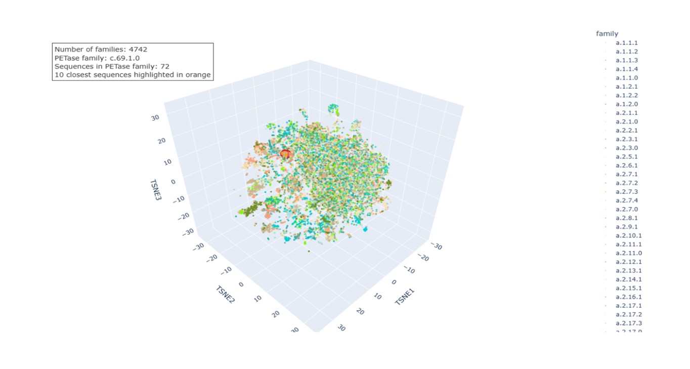
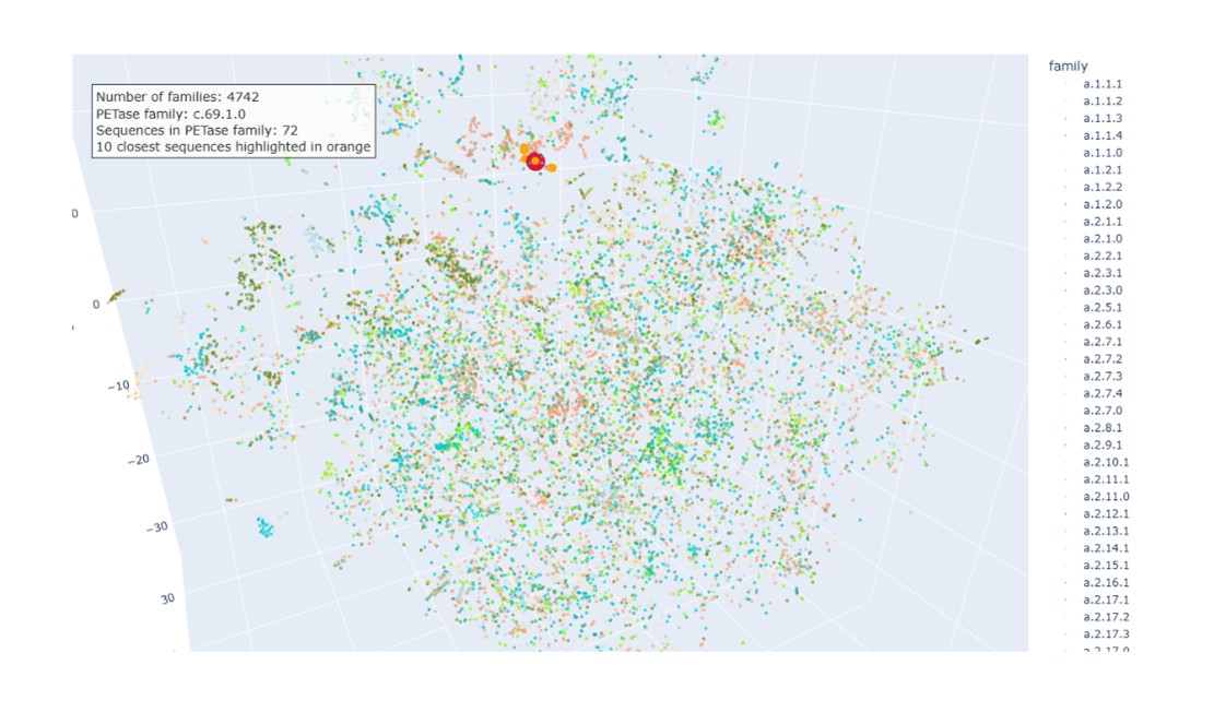
a. Use the provided sequence dataset to embed proteins in reduced dimensionality Protein embeddings were generated for each sequence using a pretrained protein language model. Each sequence was converted into a fixed-length vector by averaging the token-level representations from the final hidden layer. The embeddings were combined into a single matrix and reduced to three dimensions using t-distributed Stochastic Neighbor Embedding (t-SNE), which preserves local relationships so that proteins with similar embeddings appear close in the 3D space. In the final visualization, each protein is represented as a point and colored according to its SCOPe family classification, enabling the identification of structural or functional groups. The dataset contains 4,742 SCOPe families.

This is the link to the improved scritp in case you want to run it with your data: https://colab.research.google.com/drive/1cGdmxSwvy_ueY4OwWHuA1f7LGaTVKXWn#scrollTo=HoCzNbI7rBTL&line=5&uniqifier=1.

b. Analyze the different formed neighborhoods: do they approximate similar proteins?.
The neighborhoods observed in the t-SNE visualization correspond to groups of proteins with similar embeddings. Because the embeddings capture sequence patterns and structural information learned by the language model, proteins with similar biological characteristics tend to cluster together. This is supported by the coloring based on SCOPe families, as many clusters contain proteins from the same or closely related families, reflecting shared structural folds or evolutionary relationships.

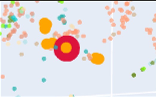
c. Place your protein (PETase) in the resulting map and explain its position and similarity to its neighbors. The PETase sequence was embedded using the same procedure as the dataset proteins and projected into the same t-SNE space. In the visualization:

• PETase highlighted in red.
• SCOPe family c.69.1.0 in salmon (72 sequences).
• Ten nearest neighbors identified by cosine similarity (orange).

PETase is located within the region occupied by members of this family, indicating that the embedding correctly captures its relationship with structurally related proteins.

The identifiers and SCOPe family annotations of the ten closest proteins are shown in the next Table:

• Dimensionality reduction also performed with UMAP, preserving both local and global structure.

Both dimensionality reduction methods produced similar but not identical results. The sets of the ten nearest proteins identified by t-SNE and Uniform Manifold Approximation and Projection overlap partially, with three sequences differing between the two top-10 lists. This difference (in yellow) arises because t-distributed Stochastic Neighbor Embedding focuses mainly on preserving local neighbor relationships, whereas UMAP attempts to preserve both local and global structure. Consequently, the overall clustering patterns are comparable, but the exact nearest neighbors of PETase vary slightly, illustrating how different dimensionality reduction methods can influence similarity interpretations.

• UMAP Script link: Colab Notebook

C2. Protein Folding

1. Folding

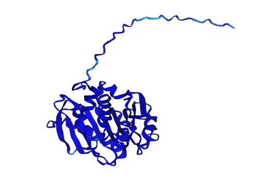
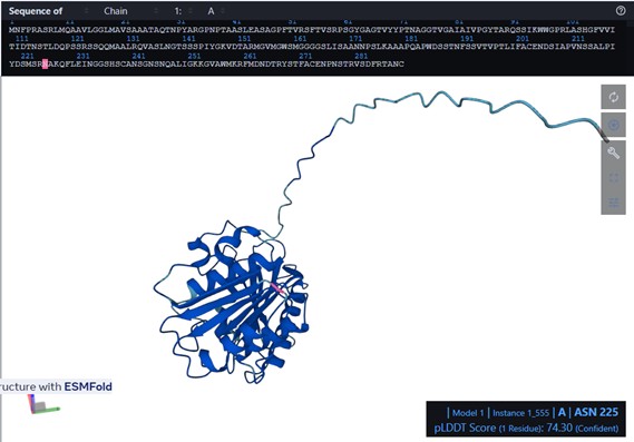
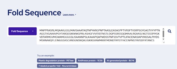
a.Fold your protein with ESMFold. Do the predicted coordinates match your original structure?

The structure was predicted with ESMFold (copies = 1, num_recycles = 3) and visualized with py3Dmol, colored by pLDDT (blue = high confidence, red = low confidence).

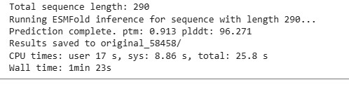
The resulting protein sequence has a total length of 290 residues. The prediction produced a pTM score of 0.913 and an average pLDDT confidence score of 96.27, indicating a high-confidence structural model.

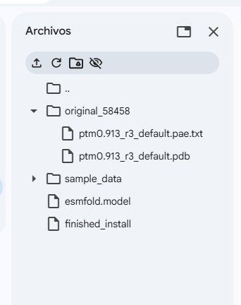
Two output files were generated. The file ptm0.913_r3_default.pdb contains the predicted three-dimensional structure of the protein, including atomic coordinates, and will be used later for structural visualization and further structural analysis. The file ptm0.913_r3_default.pae.txt contains the Predicted Aligned Error (PAE) matrix, which describes the expected positional error between residue pairs and will be referenced in a later section for model confidence evaluation.

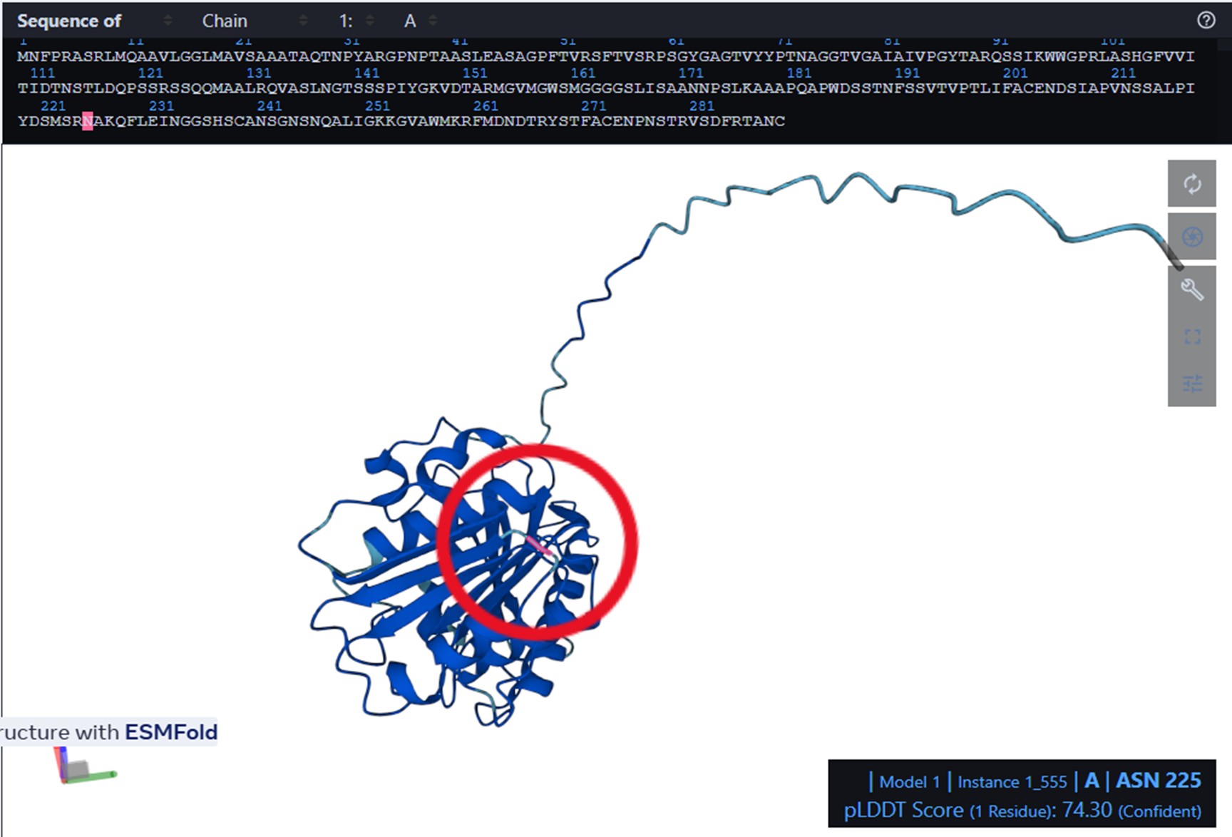
I used ESMFold in ESMatlas.com, which allows you to hover over amino acid positions in the protein and displays the confidence at that position. For example, the protein prediction shows areas in lighter blue. According to ESMAtlas (see the red circle in the next figure), this particular position (ASN 225) has a pLDDT of 74.30%. So a pLDDT of 74.3% indicates that ASN 225’s predicted position is moderately reliable, though there could be some flexibility or uncertainty in its exact placement.

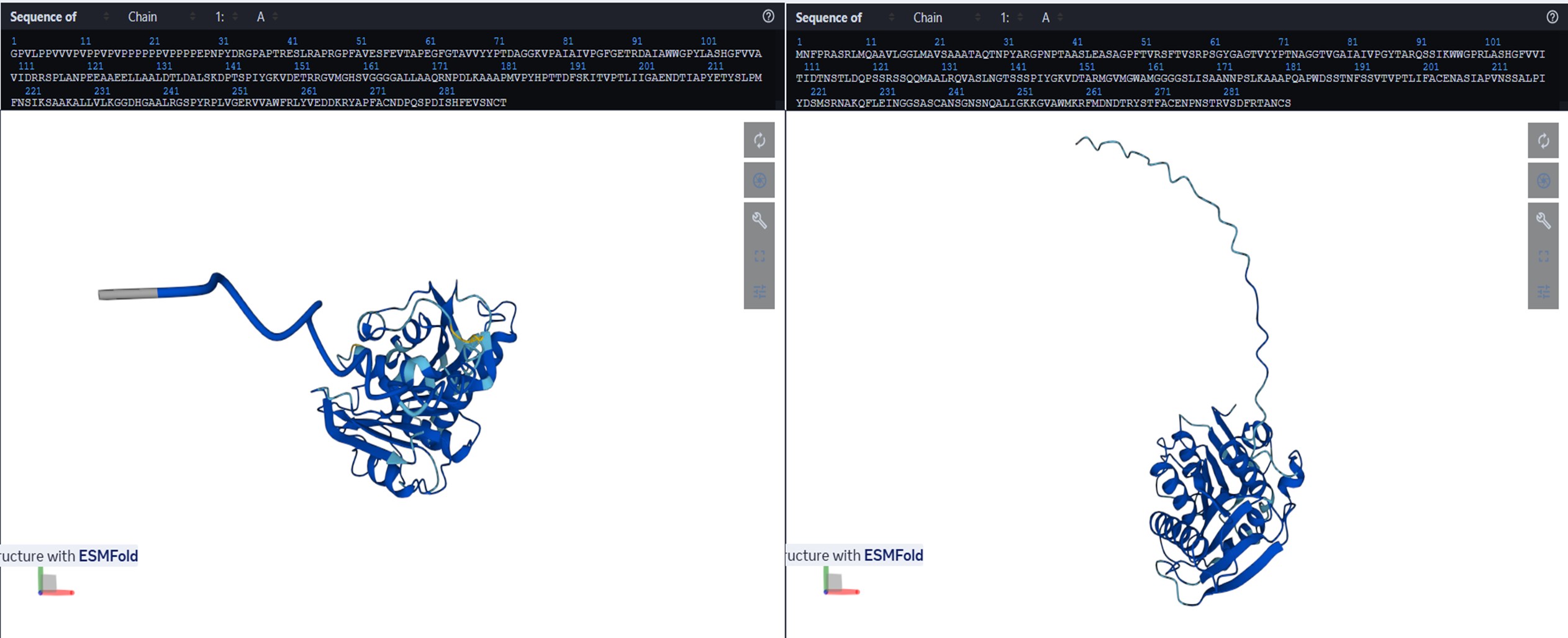
b. Try changing the sequence, first try some mutations, then large segments. Is your protein structure resilient to mutations?b) Try changing the sequence, first try some mutations, then large segments. Is your protein structure resilient to mutations?
I performed a mutation in Catalytic triad to disrupt PETase catalytic function by replacing the three key residues with alanine (S160, D206, H237):

 S160 (Serine) – nucleophile in the active site → mutated to A (Alanine)  D206 (Aspartate) – stabilizes histidine and participates in proton relay → mutated to A  H237 (Histidine) – acts as a general base in catalysis → mutated to A

(Positions are marked in red, orange arrow pointing to it; see 3 figures below, level of pLDDT included in the figure for each position before mutation.)

Sequence to be mutated and mutations positions in black:

MNFPRASRLM QAAVLGGLMA VSAAATAQTN PYARGPNPTA ASLEASAGPF TVRSFTVSRP SGYGAGTVYY PTNAGGTVGA IAIVPGYTAR QSSIKWWGPR LASHGFVVIT IDTNSTLDQP SSRSSQQMAA LRQVASLNGT SSSPIYGKVD TARMGVMGWS MGGGGSLISA ANNPSLKAAA PQAPWDSSTN FSSVTVPTLI FACENDSIAP VNSSALPIYD SMSRNAKQFL EINGGSHSCA NSGNSNQALI GKKGVAWMKR FMDNDTRYST FACENPNSTR VSDFRTANCS

With ESMFold in colab:

The mutated sequence was inserted in ESMatlas.com (ESMFold): The local changes in color reflect a reduction in confidence/pLDDT near the active site, consistent with structural perturbation. It was faster to get the level of pLDDT in ESMatlas.com (ESMFold) where I insert the mutated sequence after.

Most of the protein remains blue, but certain areas got light blue meaning that the pLDDT falls nearly below 90% of confidence. The mutations effectively target the catalytic function in the three positions without dramatically altering the overall fold.

C3. Protein Generation

Inverse-Folding a protein: Let’s now use the backbone of your chosen PDB to propose sequence candidates via ProteinMPNN.

a. Inverse protein folding with ProteinMPNN using backbone from ptm0.913_r3_default.pdb.
The input backbone for sequence design was the 3D structure predicted by ESMFold for PETase, stored in: /content/original_58458/ptm0.913_r3_default.pdb

b. Pretrained model weights v_48_020.pt were downloaded from Hugging Face.

c. Model parameters:

• Version: v_48_020
• Edges: 48
• Hidden dimension: 128
• Encoder layers: 3
• Decoder layers: 3
• Training noise: 0.2 Å
• Backbone noise: 0.0 Å

d. Native sequence evaluated: Score = 1.4683 (negative log-likelihood).

e. Designed sequence generated (temperature = 0.1):

GPVLPPVVVPVPPVPVPPPPPPVPPPPEPNPYDRGPAPTRESLRAPRGPFAVESFEVTAPEGFGTAVVYYPTDAGGKVPAIAIVPGFGETRDAIAWWGPYLASHGFVVAVIDRRSPLANPEEAAEELLAALDTLDALSKDPTSPIYGKVDETRRGVMGHSVGGGGALLAAQRNPDLKAAAPMVPYHPTTDFSKITVPTLIIGAENDTIAPYETYSLPMFNSIKSAAKALLVLKGGDHGAALRGSPYRPLVGERVVAWFRLYVEDDKRYAPFACNDPQSPDISHFEVSNCT

f. ProteinMPNN predicts the probability of each of the 21 amino acids at every position of the sequence. The predicted log-probabilities were converted into probabilities using the exponential function and averaged to obtain a position-specific probability matrix.

These probabilities were visualized using a heatmap, where: • X-axis: sequence position • Y-axis: amino acid type • Color intensity: predicted probability

Two markers were added to the heatmap: • Coral points: amino acids with the highest predicted probability at each position (ProteinMPNN prediction). • Jade points: residues from the native sequence.

This visualization allows a direct comparison between the predicted optimal sequence and the original protein sequence, which account 45% of position recovery between them.

• Script link: Colab Notebook

Questions Answered

1. Analyze predicted sequence probabilities vs original:
   ProteinMPNN predicted sequence has lower negative log-likelihood (0.7572) compared to the native (1.4683), showing higher compatibility. Heatmap highlights conserved and flexible positions, sequence recovery ~0.455.

2. Input designed sequence into ESMFold and compare:

   • Prediction visualized in esmatlas.com.
   • Predicted structure shows local variations (color differences) but overall fold largely preserved.

The ESMFold-predicted structure shows regions in light blue and yellow absent in the original. These colors reflect lower pLDDT confidence, indicating higher uncertainty or flexibility in the predicted positions. The designed sequence preserves the overall fold, but local substitutions introduce slight variability in some regions, while dark blue areas remain well-defined and conserved.

Part D. Group Brainstorm on Bacteriophage Engineering

Bacteriophage Engineering Proposal: L Protein Stabilization

Primary Goal: Increased stability (easiest).
Specific Approach: Engineering DnaJ-independence by reducing chaperone-recognition signals while preserving the structural scaffold of the L protein.

1. Computational Tools and Pipeline Justification

To achieve this goal, we propose a three-step computationally efficient pipeline:

• Step 1: Sequence-level Mutational Scanning using ESM2

  • Approach: We will perform a zero-shot in silico mutational scan across the L protein sequence using the ESM2 Protein Language Model (PLM). We aim to identify exposed hydrophobic patches (typical DnaJ recognition motifs) and propose polar/hydrophilic substitutions.
  • Why this helps: ESM2 has learned deep evolutionary constraints across millions of protein sequences. It allows us to rapidly differentiate between highly constrained residues (which are structurally vital and “untouchable”) and mutation-tolerant positions. This ensures we only disrupt chaperone-binding motifs without breaking the core evolutionary scaffold of the protein, all at a fraction of the computational cost of molecular dynamics.

• Step 2: Rapid Structural Filtering using ESMFold

  • Approach: The top candidate sequences from the ESM2 scan will be predicted using ESMFold. We will filter out any variants that collapse, show low pLDDT (confidence) scores, or have a high RMSD compared to the Wild-Type (WT) backbone.
  • Why this helps: While ESM2 evaluates sequence-level fitness, we need explicit 3D structural validation. ESMFold is significantly faster than AlphaFold2, making it ideal for high-throughput filtering. This step ensures that our hydrophilic mutations do not inadvertently destroy the L protein’s ability to fold independently.

• Step 3: Complex Modeling using Boltz-1

  • Approach: We will model the L protein + DnaJ complex for both the WT and our top folded mutant candidates. We will analyze the predicted interface contacts and Predicted Aligned Error (PAE) to assess binding affinity.
  • Why this helps: Folding correctly in isolation is not enough; we must explicitly prove reduced chaperone dependency. By comparing the mutant-DnaJ interface against the WT-DnaJ interface, we can prioritize variants that maintain a stable fold but show a significantly weakened or abolished interaction with the DnaJ chaperone.

2. Potential Pitfalls

• Pitfall 1: Overlapping Reading Frames and Genomic Constraints.
  Phage genomes are highly compact, meaning the DNA sequence encoding the L protein might also encode parts of other proteins or regulatory elements in alternative reading frames. Our targeted mutations could have unintended, fatal consequences for the phage’s overall viability. While genomic foundation models like Evo could assess these genome-wide constraints, their computational cost is prohibitive for our current scope.

• Pitfall 2: The Stability vs. Function Trade-off.
  ESMFold guarantees that the protein adopts a stable 3D conformation in solution, but it does not guarantee biological function (membrane lysis). Lytic activity heavily depends on complex factors like membrane insertion dynamics, oligomerization, and reaction kinetics. Furthermore, completely abolishing chaperone interaction might inadvertently prevent the L protein from being properly delivered to its target membrane.

Week 5 HW: Protein Design Part II

Part 1: Generate Binders with PepMLM

1. Begin by retrieving the human SOD1 sequence from UniProt (P00441) and introducing the A4V mutation.

Superoxide Dismutase 1 (SOD1) is a human enzyme that plays a critical role in protecting cells from oxidative stress by catalyzing the conversion of superoxide radicals into oxygen and hydrogen peroxide. It is a small, 154-amino-acid protein that typically forms a stable homodimer and contains a β-βarrel core structure with metal cofactors, copper and zinc, essential for its catalytic activity. Mutations in SOD1, such as the A4V variant, are associated with familial amyotrophic lateral sclerosis (ALS), a neurodegenerative disorder. SOD1 is widely expressed in the cytoplasm and is a key model protein for studying protein folding, aggregation, and targeted protein degradation strategies.

• https://www.uniprot.org/uniprot/P00441

Mutation A4V was inserted:

• Original:
  MATKAVCVLKGDGPVQGIINFEQKESNGPVKVWGSIKGLTEGLHGFHVHEFGDNTAGCTSAGPHFNPLSRKHGGPKDEERHVGDLGNVTADKDGVADVSIEDSVISLSGDHCIIGRTLVVHEKADDLGKGGNEESTKTGNAGSRLACGVIGIAQ

• Mutated:
  MATKVVCVLKGDGPVQGIINFEQKESNGPVKVWGSIKGLTEGLHGFHVHEFGDNTAGCTSAGPHFNPLSRKHGGPKDEERHVGDLGNVTADKDGVADVSIEDSVISLSGDHCIIGRTLVVHEKADDLGKGGNEESTKTGNAGSRLACGVIGIAQ

2. Using the PepMLM Colab linked from the HuggingFace PepMLM-650M model card:

3. Generate four peptides of length 12 amino acids conditioned on the mutant SOD1 sequence.

As the original script generated four peptides containing some invalid characters, I improved the script to produce only valid peptides without those characters. You can access the script cell here:

• https://colab.research.google.com/drive/1KfvaTc_AKJWRl_BQHXz-pml4H7-IPkbX#scrollTo=LMD961egloNl&line=20&uniqifier=1

Additionally, I included a scritp to calculate the pseudo-perplexity of a known peptide.

The .cvs file gives the peptides and the Pseudo Perplexity values:

Pseudo-perplexity measures the model’s confidence in a peptide sequence given the target protein context. Lower values indicate that the peptide is more consistent with patterns of protein–peptide interactions learned during training, while higher values suggest lower confidence. In the table, WRSGAAGAAWWK has the lowest pseudo-perplexity (7.12), indicating the model is most confident in this generated peptide, whereas the known binder FLYRWLPSRRGG has the highest value (20.64), reflecting comparatively lower model confidence. The other generated peptides fall in between, showing moderate confidence according to the model.

4. To your generated list, add the known SOD1-binding peptide FLYRWLPSRRGG for comparison.

• I open the test.csv file in excel, added a line and insert the SOD1-binding peptide FLYRWLPSRRGG. Record the perplexity scores that indicate PepMLM’s confidence in the binders.

PepMLM assigns lower pseudo-perplexity scores to several generated peptides compared with the known SOD1-binding peptide FLYRWLPSRRGG. The peptide WRSGAAGAAWWK shows the lowest perplexity (7.12), indicating that the model predicts it as the most probable binder among the candidates.

• https://colab.research.google.com/drive/1KfvaTc_AKJWRl_BQHXz-pml4H7-IPkbX#scrollTo=YT_adPZHhJrU&line=3&uniqifier=1

Part 2: Evaluate Binders with AlphaFold3

1. Navigate to the AlphaFold Server: alphafoldserver.com

2. For each peptide, submit the mutant SOD1 sequence followed by the peptide sequence as separate chains to model the protein-peptide complex.

3. Record the ipTM score and briefly describe where the peptide appears to bind. Does it localize near the N-terminus where A4V sits? Does it engage the β-barrel region or approach the dimer interface? Does it appear surface-bound or partially buried?

The predicted binders 1–4 localize near residues 96–102 of the protein, a region that forms one of the parallel β-strands contributing to the β-sheet structure. In contrast, the known binder (binder 5) appears near residues 11–15. None of the binders are located close to the N-terminus or C-terminus of the protein. Additionally, the peptides do not appear tightly attached to the protein surface or inserted into a binding pocket, suggesting that they remain relatively exposed rather than strongly surface-bound or buried.

The predicted interaction confidence, measured by ipTM, is relatively low for all binders, with values ranging from 0.25 to 0.44. Binder 2 shows the highest interaction score (ipTM = 0.44), followed by binder 4 (0.39) and binder 1 (0.34), while binders 3 (0.28) and 5 (0.25) show lower confidence. These values indicate moderate to low confidence in the predicted peptide–protein interactions, suggesting that the binding poses may be weak or uncertain.

4. In a short paragraph, describe the ipTM values you observe and whether any PepMLM-generated peptide matches or exceeds the known binder.

The predicted complexes show low ipTM values (0.25–0.44), indicating weak confidence in protein–peptide interactions. The PepMLM-generated peptide WRSGAAGAAWWK has the highest ipTM score (0.44), exceeding that of the known binder FLYRWLPSRRGG (0.25), but none of the peptides appear to form a stable interaction with SOD1 in the predicted models.

Part 3: Evaluate Properties of Generated Peptides in the PeptiVerse

Structural confidence alone is insufficient for therapeutic development. Using PeptiVerse, let’s evaluate the therapeutic properties of your peptide! For each PepMLM-generated peptide:

1. Paste the peptide sequence.

2. Paste the A4V mutant SOD1 sequence in the target field.

• Check the boxes:
  • Predicted binding affinity
  • Solubility
  • Hemolysis probability
  • Net charge (pH 7)
  • Molecular weight

Compare these predictions to what you observed structurally with AlphaFold3. In a short paragraph, describe what you see. Do peptides with higher ipTM also show stronger predicted affinity? Are any strong binders predicted to be hemolytic or poorly soluble? Which peptide best balances predicted binding and therapeutic properties?

Choose one peptide you would advance and justify your decision briefly.

The predicted binding affinities range from pKd/pKi values of ~5.4 to 6.9, indicating weak to moderate binding overall. The peptide WRSGAAGAAWWK shows both the highest predicted affinity (pKd 6.94) and the highest ipTM value (0.44), suggesting some agreement between the structural prediction from AlphaFold3 and the affinity prediction from Peptiverse. However, most peptides did not appear to form stable interactions with SOD1 in the structural models, remaining mostly surface-proximal rather than clearly bound. All peptides show good predicted solubility (score = 1) and very low hemolysis probabilities (<0.05), indicating favorable therapeutic properties. Among the candidates, WRSGAAGAAWWK (2) best balances predicted binding strength, structural confidence, and safety properties.

See all values from alphaFold web y pepTiVerse per peptide:

Notes:

• ipTM score estimates the confidence of protein–peptide interactions. Values above 0.7 indicate a reliable interaction, values between 0.5 and 0.7 suggest a possible interaction, and values below 0.5 indicate that an interaction is unlikely.
• Solubility is predicted as a binary value where 0 indicates not soluble and 1 indicates soluble.
• Hemolysis probability predicts whether a peptide may damage red blood cells; 0 indicates non-hemolytic and 1 indicates hemolytic.
• Binding affinity (pKd/pKi) reflects binding strength (−log10 of Kd or Ki), where higher values indicate stronger binding. Values <5 indicate very weak binding (>100 µM), 5–6 weak (~100 µM), 6–7 moderate (~10 µM), 7–8 good (~1 µM), and >8 strong binding (<100 nM).

Part 4: Generate Optimized Peptides with moPPIt

Now, move from sampling to controlled design. moPPIt uses Multi-Objective Guided Discrete Flow Matching (MOG-DFM) to steer peptide generation toward specific residues and optimize binding and therapeutic properties simultaneously. Unlike PepMLM, which samples plausible binders conditioned on just the target sequence, moPPIt lets you choose where you want to bind and optimize multiple objectives at once.

1. Open the moPPit Colab linked from the HuggingFace moPPIt model card

2. Make a copy and switch to a GPU runtime.

3. In the notebook:

1. Paste your A4V mutant SOD1 sequence.
2. Choose specific residue indices on SOD1 that you want your peptide to bind (for example, residues near position 4, the dimer interface, or another surface patch).
3. Set peptide length to 12 amino acids.
4. Enable motif and affinity guidance (and solubility/hemolysis guidance if available). Generate peptides.

4. After generation, briefly describe how these moPPit peptides differ from your PepMLM peptides. How would you evaluate these peptides before advancing them to clinical studies?

moPPIt Generated Peptides

The peptides generated with moPPIt differ from the PepMLM peptides because their generation was guided by multiple objectives defined in the notebook, including affinity, motif targeting, solubility, hemolysis, and specificity. In contrast, PepMLM generates peptides based mainly on sequence likelihood conditioned on the target protein sequence. As a result, the moPPIt peptides show moderate predicted affinities (pKd ≈ 6.2–7.2), relatively high motif scores (≈0.51–0.67), and good solubility predictions (0.75–0.92). The PepMLM peptides also show moderate affinities but were not optimized simultaneously for these therapeutic objectives during generation.

However, when one of the generated peptides was modeled with the SOD1 structure using AlphaFold, the peptide did not appear to form a stable interaction with the protein surface. This suggests that although the predicted affinity and motif scores are moderate, the structural predictions do not clearly support strong binding.

Comparison of PepMLM and moPPIt Generated Peptides

Before advancing any peptide toward clinical studies, further validation would be necessary. Additional structural modeling and docking analyses should confirm stable binding to the intended region of SOD1. Promising candidates should then be synthesized and tested experimentally through in vitro binding assays, hemolysis and cytotoxicity tests, and stability analyses to verify their predicted properties. Only peptides showing clear binding and favorable safety profiles would be considered for further development.

PENDING PENDING PENDING PENDINT

Part C: Final Project: L-Protein Mutants

High level summary: The objective of this assignment is to improve the stability and auto-folding of the lysis protein of a MS2-phage. This mechanism is key to the understanding of how phages can potentially solve antibiotic-resistance.

This homework requires computation that might take you a while to run, so please get started early.

Week 6 HW: Genetic Circuits: Part I

Answer these questions about the protocol in this week’s lab:

1. What are some components in the Phusion High-Fidelity PCR Master Mix and what is their purpose?

Components of the Phusion High-Fidelity PCR Master Mix and their purpose:

• Phusion DNA polymerase – a high-fidelity DNA polymerase that synthesizes new DNA strands with a low error rate during PCR.
• Primers (forward and reverse) – short DNA sequences that bind to the target DNA and define the region that will be amplified.
• dNTPs (dATP, dTTP, dCTP, dGTP) – the nucleotide building blocks used by the polymerase to synthesize new DNA strands.
• Reaction buffer – maintains optimal pH and ionic conditions for proper enzyme activity.
• Mg²⁺ ions – an essential cofactor required for DNA polymerase catalytic activity.
• Nuclease-free water – maintains the correct reaction volume and prevents degradation of DNA.

2. What are some factors that determine primer annealing temperature during PCR?

• Primer melting temperature (Tm) – The annealing temperature is usually set about 3–5 °C below the primer Tm to allow specific binding to the DNA template.
• Primer length – Longer primers generally have higher Tm values, which increases the annealing temperature.
• GC content – Primers with higher GC content bind more strongly (three hydrogen bonds), increasing Tm and the annealing temperature.
• Primer–template complementarity – Mismatches between the primer and the template reduce binding efficiency and may require a lower annealing temperature.
• Reaction conditions – Salt concentration and Mg²⁺ levels in the PCR mix influence DNA stability and can affect the optimal annealing temperature.

3. There are two methods from this class that create linear fragments of DNA: PCR, and restriction enzyme digests. Compare and contrast these two methods, both in terms of protocol as well as when one may be preferable to use over the other.

Comparison of PCR and Restriction Enzyme Digestion

4. How can you ensure that the DNA sequences that you have digested and PCR-ed will be appropriate for Gibson cloning?

• Design 20–40 bp complementary overhangs between adjacent DNA fragments.
• Include the correct 5′ overhangs in PCR primers so fragments share matching overlaps.
• Ensure fragments are in the correct 5′→3′ orientation for proper assembly.
• Avoid secondary structures (e.g., hairpins or primer dimers) in the overlap regions.

5. How does the plasmid DNA enter the E. coli cells during transformation?

• Heat shock: A sudden temperature change creates temporary pores in the membrane, allowing plasmid DNA to enter.
• Electroporation: An electrical pulse creates pores in the membrane through which plasmid DNA enters the cell.

6. Describe another assembly method in detail (such as Golden Gate Assembly). Explain the other method in 5 - 7 sentences plus diagrams (either handmade or online).

Golden Gate Assembly is a molecular cloning method that allows the assembly of multiple DNA fragments in a single reaction. It uses Type IIS restriction enzymes (such as BsaI) together with DNA ligase. These enzymes cut DNA outside of their recognition site, creating specific overhangs that can be designed to match between fragments. The complementary overhangs allow the DNA fragments to anneal in a predefined order. DNA ligase then joins the fragments together to form a continuous DNA molecule. Because the restriction sites are removed during the process, the final assembled DNA can no longer be cut again, making the reaction efficient and directional. This method allows the simultaneous and seamless assembly of multiple fragments in one tube.

From: (https://www.neb.com/en/nebinspired-blog/getting-started-with-golden-gate?srsltid=AfmBOopLLe5wikoDRiRJNEVt-wbJcv83I8ZyjvFnMEdyAB7CFxcSWD31)

DNA Fragment A [ATGCGTACGTTAGCTAGCTAGCGATCGATCGTAGCTAGCTAGCTA]
DNA Fragment B [AGCTATTTGCGGATCGATCA]
DNA Fragment C [ATCAGGCTAGCGTATCGTAA]

Golden Gate Assembly, Conceptual Diagram

Figure 1. pUC19 backbone

These overhangs ensure correct directional assembly of fragments A, B, and C. The sequences have been prepared and modified to include complementary overhangs for accurate Golden Gate assembly simulation in Benchling.

Golden Gate Assembly Overhangs

Fragment A → Fragment B

Fragment B → Fragment C

Overhangs’ summary

Screen shots from Benchling

Figure 1. pUC19 backbone

Figure 2. Recombinant plasmid

Figure 3. Final construct

Assignment: Asimov Kernel

1.Setup: Create a Repository and a blank Notebook entry to document the homework and save it to that Repository

2. Explore the devices in the Bacterial Demos Repo to understand how the parts work together by running the Simulator on various examples.

Demo - Represssilator

a. Construct
The repressilator construct consists of three genes (LacI, LambdaCI, and TetR) arranged in a cyclic inhibitory network. Each gene is placed under the control of a promoter that is repressed by the previous gene in the cycle. Specifically, LacI represses LambdaCI, LambdaCI represses TetR, and TetR represses LacI.
This design creates a closed loop of negative regulation, where each protein periodically inhibits the next, preventing the system from reaching a stable steady state.

b. Simulation

The RNAP flux graph shows the transcriptional activity of each gene at the final time point, indicating how strongly RNA polymerase is initiating transcription for each promoter. Differences in flux reflect variations in promoter activity within the circuit.
The RNA concentrations over time graph displays oscillatory behavior for all three genes (LacI, LambdaCI, and TetR), demonstrating periodic transcription dynamics characteristic of a repressilator system.
The ribosome flux graph represents the translation activity at the final time point, showing how actively ribosomes are producing proteins from each mRNA. Variations indicate differences in translation efficiency.
The protein concentrations over time graph shows clear oscillations in the levels of LacI, LambdaCI, and TetR. These periodic fluctuations confirm the cyclic repression mechanism, where each protein represses the next in sequence, generating sustained oscillatory behavior.

Demo - Comparing Promoters

a. Construct
This construct is designed to compare the strength of different promoters. It consists of three transcriptional units, each containing a promoter, a ribosome binding site (RBS), a reporter gene, and a terminator.
The promoters used (BBa_J23101, BBa_J23106, and BBa_J23117) have different strengths, allowing direct comparison of their effect on gene expression. Since all other components are identical, any differences in expression levels can be attributed to the promoter strength.

b. Simulation

The protein concentration graph shows three horizontal lines at different levels, each corresponding to a different gene. These steady expression levels reflect the strength of the promoters controlling each gene.
The strongest promoter produces the highest protein concentration, while the weakest promoter results in the lowest expression. Since there are no regulatory interactions between the genes, the system reaches a stable steady state without oscillations.

Demo - Multiplexer/ H1 RBS

a. Construct
The multiplexer circuit consists of multiple input signals that activate different regulatory proteins. These proteins act as repressors and interact to control the expression of the output gene (GFP).

Each input activates a specific promoter, leading to the production of regulatory proteins. These proteins then inhibit or allow the expression of the output depending on their combination. As a result, the system produces GFP only under specific input conditions, demonstrating combinatorial control of gene expression.

b. Simulation

The simulation results show that certain regulatory proteins, particularly AmtR, reach high expression levels, while others remain low. The system stabilizes without oscillations, indicating a steady-state behavior.
The protein concentration graph shows that GFP (BBa_E0040) remains at very low levels, meaning that the output is effectively repressed under these conditions. This suggests that the circuit selects a regulatory pathway that inhibits GFP expression.

Demo - AND

a. Construct
This construct implements an AND logic gate using a cascade of repressors. The inputs aTc and IPTG activate the production of regulatory proteins, which together repress an intermediate repressor. As a result, the output gene (GFP) is expressed only when both inputs are present, demonstrating conditional gene expression based on multiple signals.

This construct contains three transcription units, each controlled by promoters of different strengths: strong, medium, and weak. Each promoter drives the expression of a different reporter gene.

b. Simulation

The simulation results show that only one protein reaches a high concentration, corresponding to the output gene GFP. The other proteins remain at low levels.
The protein concentration graph reflects how promoter strength affects gene expression. Strong promoters result in higher protein levels, while weaker promoters produce lower levels of expression.
This indicates that the circuit is functioning correctly as an AND gate, where GFP is expressed only under the appropriate input conditions. The system reaches a stable steady state with clear differentiation between active and inactive components.

4. Build the Repressilator: Create a blank Construct and save it to your Repository

• Recreate the Repressilator in that empty Construct using parts from the Characterized Bacterial Parts repository
• Search the parts using the Search function in the right menu
• Drag and drop the parts into the Construct
• Confirm it works by running the Simulator (“play” button)
• Compare your results with the Repressilator Construct in the Bacterial Demos repository

A repressilator is a synthetic genetic circuit composed of three genes that inhibit each other in a cyclic manner (A represses B, B represses C, and C represses A).
This feedback loop creates oscillations in gene expression over time, meaning that the levels of each protein rise and fall periodically instead of reaching a stable state. It is a classic example of a biological oscillator in synthetic biology.

a. Construct
The repressilator construct was built by assembling three transcriptional units using parts from the characterized bacterial parts repository. Each unit consists of a promoter, a ribosome binding site (RBS), a coding sequence (CDS), and a terminator.
The genes used in this construct are LacI, LambdaCI, and TetR, arranged sequentially in the construct.

b. Expected Behavior
The repressilator is expected to exhibit oscillatory behavior in gene expression. Due to the cyclic inhibitory interactions between the three regulatory proteins, the concentration of each protein should rise and fall over time in a periodic manner.
Each gene is expressed in sequence: when one protein reaches a high level, it represses the next gene in the loop, causing its concentration to decrease, while allowing another gene to become active. This results in a continuous cycle of expression.
As a result, both RNA and protein concentrations should display sustained oscillations rather than reaching a steady state.

c. Simulation
The construct was simulated using the built-in simulator with E. coli as the chassis, a duration of 24 hours, and a timestep of 30 minutes (data for all simulations constructed).
The simulation results show that the protein concentrations increase initially and then reach a steady state without oscillations. This indicates that the system does not behave as a functional repressilator.

The simulation results show that protein concentrations increase initially and then reach a stable steady state without oscillations. All three proteins are expressed at constant levels over time.

d. Conclusion
This indicates that the constructed circuit does not function as a repressilator. The absence of oscillatory behavior is likely due to the use of identical promoters, which prevents proper regulatory interactions between the genes. As a result, the system behaves as a simple expression circuit rather than a dynamic oscillatory system.
In contrast, the repressilator in the Bacterial Demos repository shows clear oscillations, highlighting that specific regulatory promoters are required to achieve cyclic repression.

4. Build Your Own Constructs:

• Build three of your own Constructs using parts from the Characterized Bacterial Parts Repo
• Explain in the Notebook how you think each Construct should function
• Run the simulator and share your results
• If the results don’t match your expectations speculate why and try adjusting the simulator settings to achieve the expected outcome

Simple reporter (Construct 1)

a. Construct
This construct consists of a single transcriptional unit composed of a promoter, a ribosome binding site (RBS), a coding sequence (GFP), and a terminator. The promoter drives the expression of the GFP reporter gene, allowing direct observation of gene expression levels.

b. Expected behavior
This construct is expected to produce a constant level of GFP expression over time. Since there are no regulatory interactions or feedback mechanisms, the system should reach a stable steady state after an initial increase.

c. Simulation results

The simulation results show a single line corresponding to GFP protein concentration. The concentration increases rapidly at the beginning and then stabilizes, indicating that the system reaches a steady state.
The results match the expected behavior, as GFP expression increases and then stabilizes at a steady state. This confirms that the construct functions correctly without regulatory interactions.

Toggle (Construct 2)

a. Construct

b. Expected behavior
This construct is expected to behave as a toggle switch, where two genes repress each other, leading to a bistable system. Ideally, one gene should be highly expressed while the other is repressed.

c. Simulation

The simulation results show that both LacI and TetR reach similar steady-state levels. Instead of bistability, the system converges to a balanced state where both genes are expressed at comparable levels.
The lack of bistability is likely due to the symmetry of the system. Both genes are controlled by similar promoters and conditions, and no external inputs or initial differences are introduced. As a result, the system stabilizes in an intermediate state rather than switching between two distinct states.

To improve the toggle switch behavior, asymmetry was introduced by replacing the A1 RBS with a Q1 RBS for one of the genes. This change created differences in expression levels between LacI and TetR, allowing one gene to dominate over the other. As a result, the system moved away from a symmetric steady state toward partial bistable behavior.

d. Improvement- Second simulation (Q1 RBS)

The simulation shows that TetR reaches a higher concentration than LacI, indicating that the symmetry of the system has been broken. Although the system does not exhibit perfect bistability, the results demonstrate partial toggle behavior, where one gene dominates over the other.

Cascade Circuit (Construct 3)

a. Construct
This construct represents a simple genetic cascade composed of two transcriptional units. The first unit includes a constitutive promoter (PkdpF), an RBS, and the LacI coding sequence, leading to continuous production of the LacI repressor.
The second unit contains a LacI-regulated promoter (pLacI), followed by an RBS and the GFP reporter gene (BBa_E0040). In this arrangement, LacI produced in the first unit regulates the expression of GFP in the second unit, creating a one-directional regulatory cascade.

b. Expected behavior
The construct is expected to show cascade behavior, where LacI represses GFP expression through the pLacI promoter. As LacI accumulates, GFP levels decrease, and the system reaches a steady state without oscillations.

c. Simulation

The simulation results show that both LacI and GFP increase initially and then reach a steady state. LacI reaches a slightly higher concentration than GFP, indicating a weak level of repression. The small difference between the two protein levels suggests that LacI only partially reduces GFP expression.
The results partially match the expected behavior. While LacI does repress GFP, the effect is limited, and GFP is not strongly reduced. This suggests that the regulatory interaction is present but not highly efficient.

d. Improvement – Second simulation (Q1 RBS)
To improve the cascade behavior, the RBS upstream of LacI was replaced with a stronger one (Q1 RBS). This increased LacI expression and slightly enhanced repression of GFP, although the effect remains limited.

The simulation results show that both LacI and GFP increase initially and then reach a steady state. LacI reaches a significantly higher concentration than GFP, indicating a stronger level of repression. The clear separation between the two protein levels confirms that LacI effectively reduces GFP expression.
The results match the expected behavior of the cascade. As LacI accumulates, it represses GFP expression, resulting in lower GFP levels. The improvement introduced by the stronger RBS enhances this effect, making the regulatory cascade more effective.

CONCLUSION

In this work, several genetic constructs were designed and analyzed to explore different types of regulatory behavior in synthetic biology systems. The simple reporter demonstrated stable gene expression without regulation, while the repressilator highlighted the importance of specific regulatory interactions to achieve oscillatory behavior. The toggle switch showed how mutual repression can lead to bistability, and how introducing asymmetry improves its performance. Finally, the cascade circuit illustrated one-directional regulation, where adjusting expression strength enhanced control over the output gene. Overall, this work demonstrates how the design and tuning of genetic parts, such as promoters and RBS, directly influence circuit behavior, highlighting the importance of precise component selection in synthetic genetic systems.

Week 7 HW: Genetic Circuits: Part II

Week 7 — Genetic Circuits Part II: Neuromorphic Circuits

Part 1: Intracellular Artificial Neural Networks (IANNs)

1. What advantages do IANNs have over traditional genetic circuits, whose input/output behaviors are Boolean functions?

IANNs offer several advantages over traditional genetic circuits with Boolean input/output behavior:

• IANNs can process signals in a gradual way, not just ON/OFF like Boolean circuits, which makes them more flexible.
• They can perform more complex computations, instead of relying only on simple logic gates.
• They are easier to adjust, since you can change expression levels without redesigning the whole circuit.
• They handle biological noise better, because they don’t depend on strict thresholds.
• Overall, they are more powerful for modeling complex biological processes.

2. Describe a useful application for an IANN; include a detailed description of input/output behavior, as well as any limitations an IANN might face to achieve your goal.

A useful application for an IANN is as an intelligent disease-detection system inside cells. For example, it could be designed to detect early signs of cancer by sensing multiple biomarkers at the same time.

Input behavior:

• The inputs (X1, X2, etc.) would be DNA sequences that respond to different cellular signals, such as high levels of specific proteins, stress signals, or abnormal gene expression patterns.
• Each input would produce RNA and proteins through transcription and translation, and their levels would represent the strength of each signal.

Processing:

• Inside the IANN, these inputs are integrated using regulatory molecules such as endoribonucleases.
• These molecules act like weights in a neural network, enhancing or inhibiting the expression of downstream genes.
• This allows the system to combine multiple signals and make a more complex decision, rather than just a simple ON/OFF response.

Output behavior:

• The output could be the expression of a fluorescent protein or a therapeutic molecule.
• For example, if the combination of inputs matches a “disease state,” the cell would produce fluorescence (for detection) or release a drug (for treatment).

Limitations:

• Biological systems are noisy, so the response may not always be consistent.
• The processes of transcription and translation are relatively slow, which limits how fast the system can respond.
• It is also difficult to precisely control the “weights” of the network and scaling the system to include many layers or inputs can be complex.
• Additionally, interactions with other cellular processes may interfere with the circuit’s behavior.

3. Draw a diagram for an intracellular multilayer perceptron where layer 1 outputs an endoribonuclease that regulates a fluorescent protein output in layer 2.

First, before drawing the requested two-layer diagram, I will briefly explain the single-layer intracellular perceptron diagram in case it is useful to someone.

The diagram represents an intracellular single-layer perceptron where the cell processes two genetic inputs to control fluorescence output. Tx stands for transcription, the process in which DNA is copied into messenger RNA (mRNA), while Tl stands for translation, where the mRNA is used to produce a protein. Input X1 encodes the Csy4 endoribonuclease; when X1 is present, the cell transcribes and translates this gene, producing the Csy4 protein. Input X2 encodes a fluorescent protein whose mRNA can be targeted by Csy4. If only X2 is present, the fluorescent protein is produced and fluorescence is ON. However, when X1 is also present, Csy4 cuts the fluorescent mRNA, preventing translation and turning fluorescence OFF. Therefore, fluorescence is activated only when X2 is expressed without Csy4, illustrating how the cell performs a logical computation similar to a perceptron.

In contrast to the single-layer system, the intracellular multilayer perceptron introduces an additional layer of regulation before producing the final output.

The intracellular multilayer perceptron shown in the figure operates through a sequential regulatory process involving two layers of genetic computation. In the first layer, input X1 encodes an endoribonuclease. After transcription (Tx) and translation (Tl), this gene produces the regulatory protein that functions as an intermediate computational node. At the same time, input X2 encodes a fluorescent protein whose messenger RNA is generated through transcription.

The key feature of the multilayer system is that the product of layer 1 regulates the activity of layer 2. Once synthesized, the endoribonuclease recognizes and cuts the fluorescent mRNA produced from X2, preventing its translation. If X1 is absent, no regulatory enzyme is produced, allowing the fluorescent mRNA to be translated and fluorescence to be observed. Conversely, when X1 is present, the endoribonuclease suppresses translation, turning the fluorescent output OFF.

Thus, the cell performs computation in two consecutive stages: the first layer generates a regulatory signal, and the second layer determines the final observable output. This sequential control mimics the behavior of a two-layer perceptron, where an intermediate node processes input information before producing the final response.

Part 2: Fungal Materials

1. What are some examples of existing fungal materials and what are they used for? What are their advantages and disadvantages over traditional counterparts?

Fungal materials, primarily made from mycelium (the root network of fungi), are emerging as sustainable alternatives to conventional materials.

• They are used in biodegradable packaging as substitutes for plastic foam, in leather-like textiles for fashion products, in construction materials such as insulation panels and acoustic elements, and in furniture and interior design components.
• Their main advantages include renewability, biodegradability, low energy production, and the ability to grow using agricultural waste.
• They are lightweight and provide good thermal and sound insulation.

However, compared to traditional materials, fungal materials can:

• Be less durable
• Be more sensitive to moisture
• Be slower to manufacture
• Sometimes be more expensive

Large-scale production and consistent performance are still developing challenges.

2. What might you want to genetically engineer fungi to do and why? What are the advantages of doing synthetic biology in fungi as opposed to bacteria?

• Fungi could be genetically engineered to produce useful materials and solve environmental problems.
• For example, they could be modified to grow stronger biomaterials, produce medicines, create biodegradable plastics, or help break down waste and pollution.
• Scientists may also engineer fungi to make self-repairing building materials or more resistant textiles.

Advantages of using fungi compared to bacteria:

• Fungi grow as networks, which makes them good for creating large materials.
• They can release enzymes and proteins outside their cells, making production easier.
• Fungi can make more complex molecules that bacteria often cannot produce.

Limitations:

• Fungi usually grow more slowly
• Fungi are harder to modify genetically than bacteria

Overall:
Fungi are very useful for synthetic biology when complex products or materials are needed.

Assignment Part 3: First DNA Twist Order

1. Review the Individual Final Project documentation guidelines.
   Descargar informe

2. Submit this Google Form with your draft Aim 1, final project summary, HTGAA industry council selections, and shared folder for DNA designs. DUE MARCH 20 FOR MIT/HARVARD/WELLESLEY STUDENTS

3. Review Part 3: DNA Design Challenge of the week 2 homework.

• Design at least 1 insert sequence and place it into the Benchling/Kernel/Other folder you shared in the Google Form above.
• Document the backbone vector it will be synthesized in on your website.

Work flow will be as follow:

Step 1: Choose the Model Organism

For this project, we selected Escherichia coli as the model organism. It is well-studied, easy to manipulate in the lab, and has well-characterized biofilm-forming proteins. This choice allows us to design a DNA insert that promotes biofilm formation on plastic surfaces in a predictable and explainable way.

Step 2: Define the Biological Function

In this step, we selected biofilm formation as the target function, specifically focusing on initial adhesion to plastic surfaces. This function is essential because it allows bacteria to attach to the material and establish a stable biofilm, which is necessary for further activity on the surface.

Step 3: Select the Target Protein

In this step, we selected the CsgA protein from Escherichia coli. CsgA is the main structural component of curli fibers, which are extracellular protein structures involved in surface adhesion and biofilm formation. This makes it a suitable candidate for promoting attachment to plastic surfaces.

Step 4: Select the Reference Sequence

Selection of the Coding Region

Although the complete genome of Escherichia coli MG1655 is available, only the specific coding sequence (CDS) of the csgA gene was selected for this design. The full genome contains thousands of genes and non-coding regions that are not relevant to the intended function.

By isolating only the csgA CDS, we ensure that the insert contains the minimal genetic information required to produce the target protein (CsgA), which is responsible for curli fiber formation and surface adhesion. This approach simplifies the design, avoids unnecessary genetic material, and allows precise control of gene expression when the sequence is inserted into a plasmid vector.

Step 5: Design of the DNA Insert

The selected DNA insert corresponds to the coding sequence (CDS) of the csgA gene from Escherichia coli K-12 MG1655. This sequence encodes the major curlin subunit, which is the main structural component of curli fibers involved in surface adhesion and biofilm formation.

The insert was designed to include only the CDS, ensuring that it contains the minimal genetic information required to produce the target protein. This allows efficient expression when placed under the control of an appropriate promoter in a plasmid vector.

This design supports the overall objective of promoting biofilm formation on plastic surfaces, as the expression of CsgA enhances bacterial adhesion and the establishment of a stable biofilm.

Once the coding sequence was obtained in FASTA format, it was uploaded into Benchling as a linear DNA sequence for visualization and further design.

Figure 1. pUC19 backbone

Figure 2. Recombinant plasmid

Step 6: Selection of the Backbone Vector

Step 6: Selection of the Backbone Vector and Insert Integration

The pUC19 plasmid was selected as the backbone vector due to its widespread use and reliability for cloning in Escherichia coli. It contains an origin of replication, an ampicillin resistance gene, and a multiple cloning site (MCS) for DNA insertion.

The csgA coding sequence was inserted into the MCS of pUC19, specifically between the SalI and PstI restriction sites.

The resulting recombinant plasmid is expected to replicate in E. coli and enable the expression of the CsgA protein, promoting bacterial adhesion and biofilm formation on plastic surfaces.

Figure 1. pUC19 backbone

Figure 2. Recombinant plasmid

Week 9 HW: Cell Free Systems

Part A: General and Lecturer-Specific Questions

1. Explain the main advantages of cell-free protein synthesis over traditional in vivo methods, specifically in terms of flexibility and control over experimental variables. Name at least two cases where cell-free expression is more beneficial than cell production.

Cell-free protein synthesis (CFPS) has several advantages compared to in vivo methods because it is an open system and we can control everything better.

First, it gives more flexibility, because we can add or remove components directly, like DNA, enzymes or cofactors. In living cells this is more difficult because everything depends on cell conditions.

Second, we have better control of experimental variables, like temperature, ion concentration or energy levels. Also, there are no problems with cell viability.

Another important advantage is that it is faster, because we don’t need to grow cells. The reaction starts immediately.

Also, CFPS allows modification of the translation system, so we can incorporate non-natural amino acids and expand the chemical diversity of proteins beyond the 20 standard amino acids.

Cases where CFPS is more useful:

• Production of toxic proteins:
  Some proteins can kill the cell, so they cannot be produced in vivo, but in cell-free systems it is possible.

• Rapid testing of proteins or genetic systems:
  It is very useful in synthetic biology to test quickly without doing cloning and cell culture.

2. Describe the main components of a cell-free expression system and explain the role of each component.

A cell-free expression system can be understood as the core “cytoplasm” of a synthetic cell, where all the biochemical reactions needed for protein production take place. It is a fully controllable system because we can choose and adjust every component inside it, unlike in living cells.

The main component is the cell extract (lysate), which contains the molecular machinery like ribosomes, enzymes, and especially tRNAs. These tRNAs are very important because they decode the genetic information into proteins, and in cell-free systems they can even be modified to change how the genetic code is read.

Another key component is the DNA or genome, which provides the instructions to produce proteins. In synthetic systems, this genome can be minimized and fully designed depending on what proteins we want to express.

The system also includes small molecules, such as amino acids, nucleotides, and energy sources. These are essential because they act as building blocks and provide the energy needed for transcription and translation. One advantage is that we can control exactly which molecules are present, allowing us to modify the internal chemistry of the system.

Finally, although not always considered part of the core reaction, in synthetic cells this system is usually placed inside a liposome (membrane). The membrane allows compartmentalization and, together with membrane channels, enables communication with the environment, such as importing nutrients or exporting products.

In conclusion, a cell-free system is composed of the expression machinery, genetic material, and small molecules, all of which can be precisely controlled to direct protein production.

3. Why is energy provision regeneration critical in cell-free systems? Describe a method you could use to ensure continuous ATP supply in your cell-free experiment.

Energy regeneration is very important in cell-free systems because protein synthesis needs a lot of energy, mainly in the form of ATP and GTP.

Since there are no living cells, the system cannot produce energy by itself. If ATP is consumed and not regenerated, the reaction will stop very quickly and protein production will be very low.

Also, processes like transcription and translation are very energy demanding, so without a continuous energy supply, the system is not efficient.

One common method to ensure continuous ATP supply is to use an energy regeneration system, for example with phosphoenolpyruvate (PEP). In this case, PEP is used together with enzymes like pyruvate kinase to regenerate ATP from ADP.

Another option is using creatine phosphate + creatine kinase, which also helps to recycle ATP. These systems allow the reaction to continue for longer time and increase protein yield.

4. Compare prokaryotic versus eukaryotic cell-free expression systems. Choose a protein to produce in each system and explain why.

Cell-free expression systems can be divided into prokaryotic and eukaryotic, and they present important differences in terms of efficiency and protein complexity.

Prokaryotic systems, such as those based on E. coli, are usually faster, cheaper, and produce high protein yields. However, they have limitations because they cannot perform most post-translational modifications, and sometimes proteins do not fold correctly if they are complex.

In contrast, eukaryotic cell-free systems, like wheat germ, insect, or mammalian extracts, are more suitable for producing complex proteins. These systems allow post-translational modifications such as glycosylation and support proper protein folding. The disadvantage is that they are slower, more expensive, and sometimes give lower yields compared to prokaryotic systems.

An example of a protein that can be efficiently produced in a prokaryotic system is the green fluorescent protein (GFP). This protein is relatively simple, does not require complex modifications, and folds correctly in bacterial systems, so using a prokaryotic extract is more practical and efficient.

On the other hand, a good example for a eukaryotic system would be a human antibody. Antibodies require correct folding and post-translational modifications, especially glycosylation, to be functional. These processes cannot be properly carried out in prokaryotic systems, so a eukaryotic cell-free system is a better choice.

In conclusion, prokaryotic systems are ideal for simple and fast protein production, while eukaryotic systems are necessary when producing complex proteins that require modifications and proper folding.

5. How would you design a cell-free experiment to optimize the expression of a membrane protein? Discuss the challenges and how you would address them in your setup.

To optimize the expression of a membrane protein in a cell-free system, I would focus on designing an appropriate membrane environment. I would use liposomes composed of phospholipids and cholesterol, since cholesterol improves membrane fluidity and stability, which helps proper insertion of the protein.

The main challenge is that membrane proteins are hydrophobic and can aggregate if they do not interact correctly with the membrane. To address this, I would optimize the lipid composition, adjusting the ratio of phospholipids and cholesterol to create a membrane that favors correct insertion and folding.

I would also control membrane properties such as fluidity and permeability and possibly include membrane channels to allow exchange of molecules and maintain proper conditions inside the system.

In summary, optimizing the membrane composition and properties is key to avoid aggregation and ensure correct folding and functionality of the membrane protein.

6. Imagine you observe a low yield of your target protein in a cell-free system. Describe three possible reasons for this and suggest a troubleshooting strategy for each.

If a low yield of the target protein is observed in a cell-free system, there are several possible reasons related to expression efficiency, protein degradation, and folding.

First, one possible reason is inefficient transcription or translation. This can happen if the promoter is weak, the ribosome binding site is not optimal, or the codon usage is not well adapted. To solve this, the DNA can be optimized by using a strong promoter (for example T7), improving the ribosome binding site, and doing codon optimization to increase expression.

Second, protein degradation can also reduce the yield. This is usually caused by proteases present in the extract, which degrade the protein after it is produced. To solve this, we can use more purified extracts or add protease inhibitors to protect the protein.

Third, low yield can be due to incorrect protein folding or aggregation. If the protein does not fold correctly, it can become inactive or form aggregates. To improve this, we can add chaperones and adjust conditions like temperature or redox environment to help proper folding.

In conclusion, low protein yield can be caused by problems in expression, degradation, or folding, and these can be improved by optimizing the DNA and reaction conditions.

Homework question from Kate Adamala

Design an example of a useful synthetic minimal cell as follows:

1. Pick a function and describe it.

a. What would your synthetic cell do? What is the input and what is the output? The synthetic cell will detect early biofilm formation on oxygen delivery tubing and generate a visible signal to indicate contamination. The input will be quorum sensing molecules (AHL) produced by bacteria during early biofilm formation. These molecules diffuse into the synthetic cell and bind to the LuxR protein, activating gene expression. The output will be a visible signal, such as fluorescence (e.g., GFP), indicating the presence of bacterial contamination.

b. Could this function be realized by cell-free Tx/Tl alone, without encapsulation? No. Without encapsulation, the cell-free system would not be localized on the surface of the oxygen tubing, and the components could diffuse away or degrade more easily. The membrane provides compartmentalization, allowing the system to remain stable and concentrated at the site where biofilm formation occurs. This localization is important to ensure reliable detection and a clear signal in response to bacterial contamination.

c. Could this function be realized by genetically modified natural cell? Yes, this function could be achieved using genetically modified bacteria that detect quorum sensing molecules and produce a reporter signal. However, using living cells in medical devices such as oxygen tubing raises safety and regulatory concerns, including the risk of contamination or uncontrolled growth. In contrast, synthetic cells provide a safer and more controllable alternative, as they are non-living systems and can be designed to operate only under specific conditions.

d. Describe the desired outcome of your synthetic cell operation. The desired outcome is the early detection of biofilm formation on oxygen delivery tubing through a clear and visible signal. This would allow timely intervention, such as replacing or cleaning the tubing, before significant bacterial growth occurs. By providing a localized and real-time indication of contamination, the system aims to improve patient safety and reduce the risk of respiratory infections associated with biofilm formation.

2. Design all components that would need to be part of your synthetic cell.

a. What would be the membrane made of? The membrane would be composed of phospholipids (such as POPC) and cholesterol. This composition provides stability, fluidity, and biocompatibility, allowing the synthetic cell to maintain its structure while permitting diffusion of small molecules like quorum sensing signals.

b. What would you encapsulate inside? Enzymes, small molecules. The synthetic cell would encapsulate a cell-free transcription-translation (Tx/Tl) system, including ribosomes, enzymes, tRNAs, and energy components. It would also contain DNA encoding a quorum sensing detection circuit, including the LuxR protein and a reporter gene such as GFP under the control of a LuxR-activated promoter. Additionally, small molecules such as amino acids, nucleotides, and energy sources would be included to support protein expression.

c. Which organism your Tx/Tl system will come from? Is bacterial OK, or do you need a mammalian system for some reason? (hint: for example, if you want to use small molecule modulated promotors, like Tet-ON, you need mammalian) A bacterial cell-free system derived from E. coli would be used. This is suitable because the quorum sensing system (LuxR and AHL) and the reporter gene (GFP) are naturally compatible with bacterial expression systems. A mammalian system is not required, as no complex post-translational modifications or mammalian-specific regulatory elements are needed. Additionally, the system is encapsulated and immobilized within the material of the oxygen tubing, preventing direct exposure to the oxygen flow and ensuring safe operation in a medical environment.

d. How will your synthetic cell communicate with the environment? (hint: are substrates permeable? or do you need to express the membrane channel?) The synthetic cell will communicate with the environment through passive diffusion of small molecules. Quorum sensing molecules (AHL) are small and can diffuse across the lipid membrane into the synthetic cell. Inside, they activate the genetic circuit leading to reporter protein expression. The output signal, such as GFP fluorescence, does not need to exit the cell, as it can be detected externally. Therefore, no additional membrane channels are required.

3. Experimental details

a. List all lipids and genes. (bonus: find the specific genes; for example, instead of just saying “small molecule membrane channel” pick the actual gene.) Lipids: POPC (phosphatidylcholine) and cholesterol.

Genes: luxR gene encoding the quorum sensing regulator, and a reporter gene (gfp) under the control of a LuxR-activated promoter (Plux). These components enable detection of quorum sensing molecules and production of a visible fluorescence signal.

b. How will you measure the function of your system? The function of the system will be measured by detecting fluorescence from the reporter protein (GFP). Increased fluorescence intensity indicates the presence of quorum sensing molecules and activation of the synthetic cell. Fluorescence can be measured visually or using a fluorescence reader to quantify signal intensity.

Homework question from Peter Nguyen

Freeze-dried cell-free systems can be incorporated into all kinds of materials as biological sensors or as inducible enzymes to modify the material itself or the surrounding environment. Choose one application field — Architecture, Textiles/Fashion, or Robotics — and propose an application using cell-free systems that are functionally integrated into the material. Answer each of these key questions for your proposal pitch:

1. Write a one-sentence summary pitch sentence describing your concept.

I propose oxygen delivery tubing embedded with freeze-dried cell-free systems that detect early biofilm formation, trigger a visible color change, and produce enzymes to prevent microbial colonization.

2. How will the idea work, in more detail? Write 3-4 sentences or more.

The oxygen tubing would incorporate embedded freeze-dried cell-free systems immobilized within a protective matrix along the inner surface of the material. These systems would be programmed with DNA circuits that detect biofilm-associated signals, such as quorum-sensing molecules or bacterial metabolites. Upon exposure to moisture, the system activates and produces a visible color change through reporter proteins, providing an early warning of contamination. At the same time, it expresses enzymes that degrade the extracellular polymeric substances (EPS) matrix, disrupting biofilm formation. The cell-free components remain physically encapsulated within the material to prevent direct exposure to the patient while enabling localized detection and response.

3. What societal challenge or market need will this address?

Biofilm formation in oxygen delivery systems, particularly those involving humidification, poses a risk of respiratory infections and patient complications. Current prevention methods rely on strict sterilization protocols and disposable components, which increase costs and resource use. This project addresses the need for safer, self-monitoring medical devices that can detect and prevent contamination in real time, improving patient safety while reducing maintenance and waste.

4. How do you envision addressing the limitation of cell-free reactions (e.g., activation with water, stability, one-time use)?

To address the limitations of cell-free systems, the components would be encapsulated within stable, biocompatible matrices to improve durability and prevent direct exposure to the patient. Activation would be controlled by moisture present in the oxygen delivery system, ensuring the system functions only when needed. To overcome the limitation of one-time use, the tubing could incorporate replaceable or modular inner coatings that allow periodic renewal of the active components. Advances in stabilization of freeze-dried systems would further extend shelf life and maintain functionality under clinical conditions.

Homework question from Ally Huang

Freeze-dried cell-free reactions have great potential in space, where resources are constrained. As described in my talk, the Genes in Space competition challenges students to consider how biotechnology, including cell-free reactions, can be used to solve biological problems encountered in space. While the competition is limited to only high school students, your assignment will be to develop your own mock Genes in Space proposal to practice thinking about biotech applications in space!

For this particular assignment, your proposal is required to incorporate the BioBits® cell-free protein expression system, but you may also use the other tools in the Genes in Space toolkit (the miniPCR® thermal cycler and the P51 Molecular Fluorescence Viewer). For more inspiration, check out https://www.genesinspace.org/ .

1. Provide background information that describes the space biology question or challenge you propose to address. Explain why this topic is significant for humanity, relevant for space exploration, and scientifically interesting. (Maximum 100 words)

Spaceflight exposes biological systems to unique conditions, including increased radiation and microgravity, which can affect DNA stability. Telomeres are repetitive DNA sequences that protect chromosome integrity and are known to be sensitive to environmental stress and DNA damage. Changes in telomere integrity are associated with aging, genomic instability, and disease. Understanding how spaceflight conditions affect telomeric DNA is important for astronaut health during long missions. This topic is scientifically interesting because it helps us study DNA damage mechanisms in extreme environments and supports the development of safer strategies for human space exploration.

2. Name the molecular or genetic target that you propose to study. Examples of molecular targets include individual genes and proteins, DNA and RNA sequences, or broader -omics approaches. (Maximum 30 words)

Synthetic telomeric DNA sequences (TTAGGG repeats) used as a model to study telomere-associated DNA damage under spaceflight conditions.

3. Describe how your molecular or genetic target relates to the space biology question or challenge your proposal addresses. (Maximum 100 words)

The molecular target, synthetic telomeric DNA sequences, represents the repetitive regions found at the ends of chromosomes that are particularly sensitive to damage. By analyzing the integrity of these sequences after exposure to spaceflight conditions, we can assess how radiation and microgravity affect telomere stability. Since telomeres play a key role in protecting genomic DNA, damage to these regions can lead to genomic instability and cellular dysfunction. Therefore, studying telomeric DNA provides a relevant model to understand how space conditions impact DNA integrity and potential risks for astronaut health.

4. Clearly state your hypothesis or research goal and explain the reasoning behind it. (Maximum 150 words)

Spaceflight conditions, including radiation and microgravity, increase telomere-associated DNA damage compared to Earth conditions. Telomeres are repetitive DNA sequences that are particularly sensitive to environmental stress and DNA damage. In space, higher radiation levels and altered physical conditions can lead to strand breaks and base modifications, which may affect DNA integrity. Since telomeres play an important role in protecting chromosomes, damage in these regions could contribute to genomic instability and long-term health risks for astronauts.

This experiment aims to evaluate whether exposure to spaceflight conditions reduces the integrity of telomeric DNA. By comparing samples processed in space and on Earth, differences in PCR amplification and reporter expression can indicate levels of damage. This approach allows us to study DNA stability in extreme environments using a simple and controlled system.

5. Outline your experimental plan - identify the sample(s) you will test in your experiment, including any necessary controls, the type of data or measurements that will be collected, etc. (Maximum 100 words)

Identical synthetic telomeric DNA samples will be prepared and divided into Earth and spaceflight conditions. In space, samples will be processed using the miniPCR® thermal cycler to amplify telomeric sequences. PCR products will then be used as templates in the BioBits® cell-free system to express GFP. Fluorescence will be measured using the P51 Molecular Fluorescence Viewer. Earth samples will follow the same protocol as controls. Data collected will include PCR amplification efficiency and fluorescence intensity. Lower amplification and fluorescence in space samples will indicate increased telomere-associated DNA damage.

Homework Part B: Individual Final Project

Final Project Instructions

We’d like students to start exploring their final project in depth this week! Of your three Aims, for this week you should have at least Aim 1 decided and written down.

1. Put your chosen final project slide in the appropriate slide deck following the instructions on slide 1:

• MIT/Harvard/Wellesley ONE FINAL PROJECT IDEA
• Committed Listener ONE FINAL PROJECT IDEA (DONE) 2. and submit this Final Project selection form if you have not already. (DONE)

3.Begin planning how you will write your final project documentation based on these guidelines.

4. Prepare your first DNA order and put it in the “Twist (MIT)” or “Twist (Nodes)” tab of the 2026 HTGAA Ordering: DNA, Reagents, Consumables spreadsheet, as appropriate. (DONE, See below).

Final DNA Insert Design Description for twist order

The original PETase (HMW2-based) sequence from Assignment 2 was replaced with the csgA gene from Escherichia coli, aligning the design with the final project’s focus on biofilm formation. The csgA gene encodes the main structural component of curli fibers, which are essential for surface adhesion and biofilm development.

csgA Sequence

Length: 456 bp
Description: Coding sequence including start and stop codons

ATGAAACTTTTAAAAGTAGCAGCAATTGCAGCAATCGTATTCTCCGGTAGCGCTCTGGCAGGTGTTGTTCCTCAGTACGGCGGCGGCGGTAACCACGGTGGTGGCGGTAATAATAGCGGCCCAAATTCTGAGCTGAACATTTACCAGTACGGTGGCGGTAACTCTGCACTTGCTCTGCAAACTGATGCCCGTAACTCTGACTTGACTATTACCCAGCATGGCGGCGGTAATGGTGCAGATGTTGGTCAGGGCTCAGATGACAGCTCAATCGATCTGACCCAACGTGGCTTCGGTAACAGCGCTACTCTTGATCAGTGGAACGGCAAAAATTCTGAAATGACGGTTAAACAGTTCGGTGGTGGCAACGGTGCTGCAGTTGACCAGACTGCATCTAACTCCTCCGTCAACGTGACTCAGGTTGGCTTTGGTAACAACGCGACCGCTCATCAGTACTAA

The insert was designed as a complete expression cassette, including a constitutive promoter (BBa_J23106), a ribosome binding site (RBS, GCCACC), an ATG start codon, the csgA coding sequence, a TAA stop codon, and a BBa_B0015 double terminator to ensure proper transcription and translation in E. coli.

For cloning and propagation, the backbone vector selected is pUC19, chosen for its high copy number, ampicillin resistance marker, and well-characterized multiple cloning site.

Figure 1. pUC19 backbone

Figure 2. Recombinant plasmid

The designed insert sequence can be accessed here: Benchling sequence link.

Week 10 HW: Advanced Imaging & Measurement Technology

PART A: Final Project

1. Please identify at least one (ideally many) aspect(s) of your project that you will measure. It could be the mass or sequence of a protein, the presence, absence, or quantity of a biomarker, etc.

In this project, it would be recommended to measure several aspects related to microbial adhesion proteins involved in biofilm formation on microplastics. These include the molecular weight and amino acid sequence of candidate adhesion proteins, as well as their relative abundance. It would also be useful to measure the presence and quantity of biofilm formation on synthetic polymer surfaces. Additionally, evaluating protein–surface interactions, such as binding affinity to plastics, would provide insight into adhesion mechanisms. Finally, physicochemical properties such as hydrophobicity and surface charge could be analyzed, as they are known to influence protein adhesion behavior.

Please describe all of the elements you would like to measure, and furthermore describe how you will perform these measurements.

In this project, I would like to measure several elements related to microbial adhesion proteins and biofilm formation on microplastics. First, I would like to determine the molecular weight and amino acid sequence of candidate adhesion proteins using liquid chromatography–mass spectrometry (LC-MS). This would involve digesting the proteins with trypsin to generate peptides, followed by separation using liquid chromatography and analysis by mass spectrometry to obtain mass-to-charge ratios and reconstruct the protein sequence.

I would also like to investigate protein structure and folding using native and denatured mass spectrometry. By comparing the charge state distributions under different conditions, I could infer differences in protein conformation and stability.

Additionally, I would like to measure protein–surface interactions by performing adhesion assays, where proteins are incubated with synthetic polymer surfaces and the amount of bound protein is quantified.

I would also like to evaluate biofilm formation using assays such as crystal violet staining to quantify biomass attached to surfaces.

Finally, I would like to analyze physicochemical properties such as hydrophobicity and surface charge using computational tools, as these factors influence protein adhesion behavior.

3. What are the technologies you will use (e.g., gel electrophoresis, DNA sequencing, mass spectrometry, etc.)? Describe in detail.

In this project, I would use several complementary analytical and experimental technologies to study microbial adhesion proteins and biofilm formation.

First, I would use liquid chromatography–mass spectrometry (LC-MS) to analyze protein molecular weight and amino acid sequence. Proteins would be digested with trypsin into peptides, which would then be separated by liquid chromatography and analyzed by mass spectrometry to determine their mass-to-charge ratios. Tandem mass spectrometry (MS/MS) would be used to fragment peptides and reconstruct their amino acid sequences.

I would also use native and denatured mass spectrometry to investigate protein structure and folding. By comparing charge state distributions under different conditions, this technique allows for the analysis of protein conformation and structural stability.

To study protein–surface interactions, I would use adhesion assays, where proteins are incubated with microplastic surfaces and the amount of bound protein is measured.

For biofilm quantification, I would use a crystal violet staining assay, which measures the total biomass attached to a surface through absorbance.

Additionally, I would use computational tools for sequence analysis and structure prediction, such as bioinformatics software and protein modeling platforms, to evaluate properties like hydrophobicity, charge, and predicted 3D structure.

Together, these technologies provide a comprehensive approach to analyzing protein identity, structure, and function in biofilm formation.

Waters Part I — Molecular Weight

1. Calculation of Molecular Weight for eGFP

Based on the predicted amino acid sequence of eGFP (see below) and any known modifications, what is the calculated molecular weight? You can use an online calculator such as:

https://web.expasy.org/compute_pi/

MVSKGEELFTG VVPILVELDG DVNGHKFSVS GEGEGDATYG KLTLKFICTT
GKLPVPWPTL VTTLTYGVQC FSRYPDHMKQ HDFFKSAMPE GYVQERTIFF
KDDGNYKTRA EVKFEGDTLV NRIELKGIDF KEDGNILGHK LEYNYNSHNV
YIMADKQKNG IKVNFKIRHN IEDGSVQLAD HYQQNTPIGD GPVLLPDNHY
LSTQSALSKD PNEKRDHMVL LEFVTAAGIT LGMDELYKLE HHHHHH

Note: This contains a His-purification tag (HHHHHH) and a linker (the LE before it).

The sequence was inserted into the ExPASy calculator and obtained a molecular weight of 28,006.60 Da and an isoelectric point (pI) of 5.90. The molecular weight indicates the total mass of the protein, including the initiator methionine (M), the C-terminal His-tag (HHHHHH), and the linker sequence (LE) present in the construct. The isoelectric point indicates the pH at which the protein has no net charge.

2. Calculate the molecular weight of the eGFP using the adjacent charge state approach described in the recitation. Select two charge states from the intact LC-MS data (Figure 1) and:

Figure 1. Mass Spectrum of intact eGFP protein from the Waters Xevo G3 LC-MS (a mass spectrometer with 30,000 resolution) with individual charge state peaks labeled with m/z values.

2.1 determine z for each adjacent pair of peaks (n, n+1) using:

To determine the charge state (z) from adjacent peaks, the relationship between two consecutive charge states (n and n+1) is used, including the exact proton mass (mH = 1.007276 Da):

z = (m/zₙ₊₁ − mH) / (m/zₙ − m/zₙ₊₁)

Using two adjacent peaks from the spectrum:

m/zₙ = 848.9758
m/zₙ₊₁ = 875.4421

Substituting:

z = (875.4421 − 1.007276) / (848.9758 − 875.4421)

z = 874.4348 / (−26.4663)

z ≈ −33.06

Since the charge state cannot be negative, the absolute value is taken:

z ≈ 33.06

So, the peak at m/z = 848.98 corresponds to a charge state of +33, and the adjacent peak at m/z = 875.44 corresponds to +32.

The term mH = 1.007276 Da corresponds to the mass of a proton (H⁺). In electrospray ionization (ESI), proteins gain protons to become positively charged ions, written as [M + zH]ᶻ⁺. Each proton adds both one positive charge and a small amount of mass (~1.007276 Da). For this reason, this value is included in the equation.

The negative value obtained comes from the order of the m/z values in the denominator and does not have physical meaning.

2.2 Determine the molecular weight (MW) of the protein using the relationship between m/zₙ, MW, and z.

The molecular weight (MW) of the protein is calculated using the relationship:

MW = (z × m/zₙ) − z

Using the determined charge state:

z ≈ 33.06
m/zₙ = 848.9758

Substituting:

MW = (33.06 × 848.9758) − 33.06

MW = 28067.15 − 33.06

MW ≈ 28,034.09 Da

Therefore, the molecular weight of the protein is approximately 28.03 kDa, which is consistent with the expected mass of eGFP.

This calculation uses a simplified approach assuming a proton mass of approximately 1 Da, which is sufficient for this analysis.

2.3 Calculate the accuracy of the measurement using the deconvoluted MW from 2.2 and the predicted weight of the protein from 2.1 using:

The mass accuracy is calculated using the following expression:

ppm error = (|MW_exp − MW_theo| / MW_theo) × 10^6

Using the obtained values:

MW_exp = 28,034.09 Da
MW_theo = 28,006.60 Da

Substituting:

ppm = (|28,034.09 − 28,006.60| / 28,006.60) × 10^6

ppm = (27.49 / 28,006.60) × 10^6

ppm ≈ 981 ppm

Therefore, the mass accuracy is approximately 981 ppm.

This value is significantly higher than the acceptable range of 30–50 ppm, which suggests that there may be an error in the calculation or that the selected peaks were not optimal for determining the charge state.

2.4 Can you observe the charge state for the zoomed-in peak in the mass spectrum for the intact eGFP? If yes, what is it? If no, why not? No, the charge state cannot be directly observed from the zoomed-in peak at ~1470 m/z.

In the zoomed region, the signal appears as a broad peak without resolved isotopic structure. Since the isotopic peaks are not visible, it is not possible to determine the charge state using isotopic spacing (which would require resolving peaks separated by 1/z).

Additionally, this peak does not follow the main charge state distribution observed in the spectrum, as it appears isolated and does not form part of a consistent series of adjacent charge states.

Therefore, the charge state cannot be determined directly from this peak, and it is likely due to a different species (such as a contaminant or adduct) rather than the main protein signal.

Waters Part II — Secondary/Tertiary structure

We will analyze eGFP in its native, folded state and compare it to its denatured, unfolded state on a quadrupole time-of-flight MS. We will be doing MS-only analysis (no liquid chromatography, also known as “direct infusion” experiments) on the Waters Xevo G3-QToF MS.

1. Based on learnings in the lab, please explain the difference between native and denatured protein conformations. For example, what happens when a protein unfolds? How is that determined with a mass spectrometer? What changes do you see in the mass spectrum between the native and denatured protein analyses (Figure 2)?

Figure 2. Comparison of the mass spectra between denatured (top) and native (bottom) eGFP standard on the Waters Xevo G3 QTof MS.

Native proteins have a compact and well-folded structure, while denatured proteins are unfolded and more extended. When a protein unfolds, its higher-order structure is disrupted, which increases the exposed surface area.

This structural change affects how the protein is ionized in electrospray ionization (ESI). In the native state, fewer protonation sites are accessible, so the protein acquires fewer charges. In contrast, in the denatured state, more surface area is exposed, allowing more protonation sites and resulting in higher charge states.

This difference is clearly observed in the mass spectrum. Native proteins show a narrow charge state distribution with lower charge states (higher m/z values), indicating a more uniform and stable conformation. On the other hand, denatured proteins show a broader charge state distribution with higher charge states (lower m/z values), reflecting increased conformational heterogeneity.

In Figure 2, the denatured protein (top) shows peaks shifted to lower m/z values, corresponding to higher charge states, while the native protein (bottom) shows peaks at higher m/z values with fewer charge states. Additionally, the denatured spectrum is more spread out, indicating the presence of multiple conformations in solution.

Therefore, the charge state distribution and peak position in the mass spectrum provide information about both the folding state and the conformational dynamics of the protein.

2. Zooming into the native mass spectrum of eGFP from the Waters Xevo G3 QTof MS (see Figure 3), can you discern the charge state of the peak at ~2800 m/z? What is the charge state? How can you tell?

Figure 3. Native eGFP mass spectrum from the Waters Xevo G3 Q-Tof MS. The inset is a zoomed-in view of the charge state at ~2800 m/z on a mass spectrometer with 30,000 resolution.

No, the charge state of the peak at ~2800 m/z cannot be directly determined.

Although the peak at approximately 2799 m/z is clearly visible in the spectrum, there is no resolved isotopic structure shown for this peak. Without visible isotopic spacing, it is not possible to determine the charge state using the relationship spacing = 1/z.

In contrast, another peak around ~2545 m/z shows clear isotopic resolution, which would allow charge determination. However, for the ~2800 m/z peak, this information is not available.

Therefore, the charge state cannot be directly determined from this peak.

REVISAR REVISAR REVISAR REVISAR

NO ESTOY SEGURA DE ESTO.

Waters Part III — Peptide Mapping - primary structure

We will digest the eGFP protein standard into peptides using trypsin (an enzyme that selectively cleaves the peptide bond after Lysine (K) and Arginine (R) residues. The resulting peptides will be analyzed on the Waters BioAccord LC-MS to measure their molecular weights and fragmented to confirm the amino acid sequence within each peptide – generating a “peptide map”. This process is used to confirm the primary structure of the protein.

There are a variety of tools available online to calculate protein molecular weight and predict a list of peptides generated from a tryptic digest. We will be using tools within the online resource Expasy (the bioinformatics resource portal of the Swiss Institute of Bioinformatics (SIB)) to predict a list of tryptic peptides from eGFP.

1. How many Lysines (K) and Arginines (R) are in eGFP? Please circle or highlight them in the eGFP sequence given in Waters Part I question 1 above. (Note: adding the sequence to Benchling as an amino acid file and clicking biochemical properties tab will show you a count for each amino acid).

MVSKGEELFTG VVPILVELDG DVNGHKFSVS GEGEGDATYG KLTLKFICTT GKLPVPWPTL VTTLTYGVQC FSRYPDHMKQ HDFFKSAMPE GYVQERTIFF KDDGNYKTRA EVKFEGDTLV NRIELKGIDF KEDGNILGHK LEYNYNSHNV YIMADKQKNG IKVNFKIRHN IEDGSVQLAD HYQQNTPIGD GPVLLPDNHY LSTQSALSKD PNEK****RDHMVL LEFVTAAGIT LGMDELYKLE HHHHHH

The eGFP amino acid sequence was analyzed to determine the number of trypsin cleavage sites. Trypsin specifically cleaves peptide bonds at the C-terminal side of Lysine (K) and Arginine (R) residues.

• Total number of Lysine (K) residues: 20
• Total number of Arginine (R) residues: 6

These residues represent the potential cleavage sites and define the set of peptides generated during tryptic digestion.

2. How many peptides will be generated from tryptic digestion of eGFP?

• Navigate to https://web.expasy.org/peptide_mass/
• Copy/paste the sequence above into the input box in the PeptideMass tool to generate expected list of peptides.
• Use Figure 4 below as a guide for the relevant parameters to predict peptides from eGFP.

Figure 4. Example conditions for predicting the number of tryptic peptides from the eGFP standard. Please replicate all parameters shown above.

• Click “Perform the Cleavage” button in the PeptideMass tool and report the number of peptides generated when using trypsin to perform the digest.

Using the ExPASy PeptideMass tool with the specified parameters (trypsin digestion, 0 missed cleavages, and peptides > 500 Da), a total of 19 peptides were generated from the eGFP sequence.

Although the sequence contains 20 Lysine (K) and 6 Arginine (R) residues (26 potential cleavage sites), the number of observed peptides is lower due to several factors:

• Mass filtering (> 500 Da):
  Peptides with a molecular weight below 500 Da are excluded based on the selected parameters. Therefore, some cleavage products are not included in the final count.

• Trypsin cleavage rules:
  Trypsin cleaves at the C-terminal side of K and R residues; however, cleavage efficiency can be affected by sequence context (e.g., steric hindrance or neighboring residues).

• Terminal peptides:
  The number of resulting peptides is not always equal to the number of cleavage sites, as the protein sequence generates one additional peptide fragment at the N- and C-termini.

Overall, the reported number of peptides reflects both the enzymatic specificity of trypsin and the filtering criteria applied during the in silico digestion.

In addition to determining the number of peptides generated, the ExPASy PeptideMass tool provides the theoretical monoisotopic masses of each tryptic fragment. Under the specified conditions (trypsin digestion, 0 missed cleavages, peptides > 500 Da), the following peptide masses (Da) for a total of 19 peptides were obtained:

The sum of these peptide masses accounts for the majority of the protein sequence, consistent with the reported 90.7% sequence coverage. The small fraction of missing mass corresponds to peptides below the 500 Da threshold, which were excluded based on the selected parameters.

This peptide mass distribution reflects the expected outcome of trypsin digestion, where cleavage at Lysine (K) and Arginine (R) residues generates a set of peptides with predictable sizes and masses. The agreement between the theoretical digestion and the observed peptide masses supports the accuracy of the sequence and the digestion model.

Overall, this analysis demonstrates how peptide mapping enables verification of protein primary structure through the comparison of predicted and experimentally observed peptide masses.

3. Based on the LC-MS data for the Peptide Map data generated in lab (please use Figure 5a as a reference) how many chromatographic peaks do you see in the eGFP peptide map between 0.5 and 6 minutes? You may count all peaks that are >10% relative abundance.

Figure 5a. Total ion chromatogram (TIC) of the eGFP peptide map. The peak at 2.78 minutes is circled, and its MS data is shown in the mass spectrum in Figure 5b, below.

Based on the LC-MS data shown in Figure 5a, the chromatographic peaks between 0.5 and 6.0 minutes were analyzed. A threshold of 10% relative abundance was applied, corresponding to approximately 1.2 × 10⁶ TIC counts.

Only peaks exceeding this threshold were considered for the analysis. After carefully examining the chromatogram, the following peaks were identified:

• 0.61 min, 0.79 min, 1.43 min, 1.80 min, 1.85 min
• 1.93 min, 2.17 min, 2.26 min, 2.54 min, 2.78 min
• 3.27 min, 3.53 min, 3.59 min, 3.70 min, 4.48 min
• 4.64 min, 4.87 min

In total, 17 chromatographic peaks above the 10% relative abundance threshold were observed within the selected retention time window.

Peaks such as 4.30, 5.06, and 5.43 minutes were excluded, as their intensities were below the defined threshold.

This analysis reflects the main peptide fragments detected in the eGFP digest under the given LC-MS conditions.

4. Assuming all the peaks are peptides, does the number of peaks match the number of peptides predicted from question 2 above? Are there more peaks in the chromatogram or fewer?

Based on the in silico digestion results from Question 2, a total of 19 peptides were predicted.

From the LC-MS chromatogram analysis (Figure 5a), approximately 17 chromatographic peaks above the 10% relative abundance threshold were observed between 0.5 and 6 minutes.

Therefore, the number of observed peaks is slightly lower than the number of predicted peptides.

This difference can be explained by several factors:

• Some peptides may not be detected due to poor ionization efficiency.
• Certain peptides may be present at low abundance and fall below the detection threshold.
• Co-elution of peptides may result in overlapping peaks that are not resolved as separate signals.
• Experimental limitations in LC-MS detection can also contribute to missing signals.

Overall, the chromatogram shows fewer peaks than the theoretically predicted peptides.

5. Identify the mass-to-charge (m/z) of the peptide shown in Figure 5b. What is the charge (z) of the most abundant charge state of the peptide (use the separation of the isotopes to determine the charge state). Calculate the mass of the singly charged form of the peptide ([M+H]+) based on its m/z and z.

Figure 5b. Mass spectrum figure to show for the chromatographic peak at 2.78 min from Figure 5a above. The inset is a zoom-in of the peak at m/z 525.76, to discern the isotope peaks.

The most intense peak in the mass spectrum is observed at m/z ≈ 525.77, corresponding to the most abundant charge state of the peptide.

Determination of the Charge State (z)

From the zoomed-in isotope pattern, the following consecutive peaks were observed:

525.76712, 526.25918, 526.76845, 527.26098

The spacing between peaks was calculated as:

526.25918 − 525.76712 = 0.49206
526.76845 − 526.25918 = 0.50927
527.26098 − 526.76845 = 0.49253

These values give an average Δ(m/z) ≈ 0.50.

Using the relationship:

z = 1 / Δ(m/z)

z ≈ 1 / 0.50 = 2

Therefore, the peptide has a charge state of z = +2.

Calculation of the Singly Charged Mass [M+H]⁺

In mass spectrometry, the observed m/z is related to the peptide mass by:

m/z = (M + zH) / z

Where:

• M = neutral mass of the peptide
• H = mass of a proton ≈ 1.007 Da
• z = charge state

Rearranging:

M = (m/z × z) − (z × H)

The singly charged form is:

[M+H]⁺ = M + H
[M+H]⁺ = (m/z × z) − (z − 1) × H

Substituting the values:

m/z = 525.77
z = 2
H = 1.007 Da

[M+H]⁺ = (525.77 × 2) − (2 − 1) × 1.007
[M+H]⁺ = 1051.54 − 1.007
[M+H]⁺ ≈ 1050.53 Da

The peptide has:

• m/z ≈ 525.77
• charge state z = +2
• calculated singly charged mass [M+H]⁺ ≈ 1050.53 Da

This result is further supported by the presence of a peak at m/z ≈ 1050.52 in the fragmentation spectrum (Figure 5c), corresponding to the singly charged form of the same peptide.

6. Identify the peptide based on comparison to expected masses in the PeptideMass tool. What is mass accuracy of measurement? Please calculate the error in ppm. (Recall that Accuracy = |MW experiment - MW theory|/MW theory

The peptide was identified by comparing the experimentally determined mass with the theoretical masses obtained from the PeptideMass tool.

The observed singly charged mass was approximately 1050.53 Da, which matches closely with the theoretical mass of 1050.5214 Da for the peptide FEGDTLVNR (positions 115–123).

Error (ppm) was calculated using:

Error (ppm) = |MW_exp − MW_theory| / MW_theory × 10^6

Substituting the values:

|1050.53 − 1050.5214| = 0.0086

Error = (0.0086 / 1050.5214) × 10^6

Error ≈ 8.19 ppm

The peptide is identified as FEGDTLVNR, and the mass accuracy of the measurement is approximately 8.2 ppm, indicating a good agreement between experimental and theoretical values.

7. What is the percentage of the sequence that is confirmed by peptide mapping? (see Figure 6)

Figure 6. Amino Acid Coverage Map of eGFP based on BioAccord LC-MS peptide identification data.

Based on Figure 6, the percentage of the protein sequence confirmed by peptide mapping is 88%.

This value represents the sequence coverage obtained from the identified peptides, indicating that the majority of the protein sequence was successfully detected and validated.

Bonus Peptide Map Questions

8. Can you determine the peptide sequence for the peptide fragmentation spectrum shown in Figure 5c? (HINT: Use your results from Question 2 above to match the peptide molecular weight that is closest to that shown in Figure 5b. Copy and paste its sequence into this tool online to predict the fragmentation pattern based on its amino acid sequence: http://db.systemsbiology.net/proteomicsToolkit/FragIonServlet.html. What is the sequence of the eGFP peptide that best matches the fragmentation spectrum in Figure 5c?

Figure 5c. Fragmentation spectrum of the peptide eluting at retention time 2.78 minutes in Figure 5a (above).

To determine the peptide sequence corresponding to the fragmentation spectrum (Figure 5c), the following approach was used:

a. The experimental mass of the peptide was first determined from Figure 5b, where the singly charged ion was observed at approximately 1050.52 Da.

b. This value was compared with the theoretical peptide masses obtained in Question 2. The closest match corresponded to the peptide:

FEGDTLVNR (MW = 1050.5214 Da) (answer question 6).

c. To validate this assignment, the peptide sequence was entered into the Fragment Ion Calculator (Proteomics Toolkit), selecting:

• Monoisotopic mass
• Charge state +1
• b- and y-ions

d. The predicted fragmentation pattern (b- and y-ions) was then compared to the experimental MS/MS spectrum (Figure 5c).

Results: Fragment Ion Comparison

The red circles in Figure 5c correspond to the theoretical peaks that match the observed ones.

Interpretation:

The comparison between the theoretical and experimental fragmentation data shows a good agreement.

The main y-ion series (y9, y8, y7) matches very well with the observed peaks, with only very small differences in m/z values. These differences are very low and acceptable in LC-MS/MS experiments.

Other ions such as y5, y4 and y3 also match the spectrum, although some of them appear with lower intensity. This still supports the identification of the peptide.

Some ions (y6, y2, y1) are not observed, but this is normal in fragmentation experiments. It can be due to low intensity, inefficient fragmentation, or signals below the detection limit.

Overall, the presence of several matching y-ions confirms the peptide sequence.

Additional Peaks

Some peaks in the spectrum do not match the predicted y-ions of the peptide FEGDTLVNR.

These peaks may come from:

• b-ions or other fragment ions
• background noise
• small impurities or co-eluting peptides

These additional peaks do not affect the identification, since the main y-ion series is clearly observed.

Conclusion: The peptide sequence that best matches the fragmentation spectrum is FEGDTLVNR

The good agreement between theoretical and experimental fragment ions confirms the correct identification of the peptide.

9. Does the peptide map data make sense, i.e. do the results indicate the protein is the eGFP standard? Why or why not? Consult with Figure 6, which depicts the % amino acid coverage of peptides positively identified using their calculated mass and fragmentation pattern.

The peptide map data is consistent with the expected results for the eGFP standard.

According to Figure 6, the sequence coverage is approximately 88%, which is a relatively high value. This means that most of the protein sequence has been successfully identified.

In addition, the peptides were confirmed using both their calculated mass and their fragmentation patterns, which increases the confidence in the identification.

Even though the coverage is not 100%, this is normal in LC-MS/MS experiments. Some peptides may not be detected due to low intensity, poor ionization, or limitations in the experimental method.

Overall, the results make sense and strongly suggest that the protein analyzed corresponds to the eGFP standard.

Waters Part IV — Oligomers

We will determine Keyhole Limpet Hemocyanin (KLH)’s oligomeric states using charge detection mass spectrometry (CDMS). CDMS single-particle measurements of KLH allow us to make direct mass measurements to determine what oligomeric states (that is, how many protein subunits combine) are present in solution. Using the known masses of the polypeptide subunits (Table 1) for KLH, identify where the following oligomeric species are on the spectrum shown below from the CDMS (Figure 7): 7FU Decamer 8FU Didecamer 8FU 3-Decamer 8FU 4-Decamer

Figure 7. Mass spectrum of Keyhole Limpet Hemocyanin (KLH) acquired on the CDMS.

The oligomeric states of KLH can be determined based on multiples of a decamer unit, where one decamer corresponds to 10 protein subunits.

Using the known subunit masses:

• 7FU = 340 kDa
• 8FU = 400 kDa

The expected masses are:

• 7FU Decamer (10 subunits)
  10 × 340 kDa = 3400 kDa = 3.4 MDa

• 8FU Didecamer (20 subunits)
  20 × 400 kDa = 8000 kDa = 8.0 MDa

• 8FU 3-Decamer (30 subunits)
  30 × 400 kDa = 12000 kDa = 12.0 MDa

• 8FU 4-Decamer (40 subunits)
  40 × 400 kDa = 16000 kDa = 16.0 MDa

In the CDMS spectrum (Figure 7), these oligomeric species can be identified at the corresponding mass values. The peaks circled in red match closely with the expected masses:

• A peak at ~3.4 MDa corresponds to the 7FU decamer
• A strong peak at ~8.3 MDa corresponds to the 8FU didecamer
• A peak at ~12.7 MDa corresponds to the 8FU 3-decamer
• A weaker signal near ~16 MDa corresponds to the 8FU 4-decamer

The small differences between theoretical and observed masses are likely due to experimental variation and instrument resolution.

Overall, the spectrum clearly shows multiple oligomeric states of KLH in solution, confirming the presence of different assemblies formed by combinations of its subunits.

Waters Part V — Did I make GFP?

Please fill out this table with the data you acquired from the lab work done at the Waters Immerse Lab in Cambridge, or else the data screenshots in this document if you were unable to have lab work done at Waters.

Molecular Weight Comparison (eGFP)

Week 11 HW: Bioproduction & Cloud Labs

Cloud laboratories are making science accessible, affordable, and reproducible. Our aim this semester is to showcase how they can enable human creativity at scale, and how they provide a platform for collaboration and community.

How To Grow (Almost) Anything is about synthetic biology, bioengineering, robotics, automation, art, and AI. But it is also about friendship, shared purpose, and the freedom to build beyond what we know and to be inspired by what can be. To that end, the goal with this cloud lab unit and homework assignment is to inspire collaboration and creativity while designing a scientifically rigorous cell-free fluorescent protein optimization experiment together.

Part A: The 1,536 Pixel Artwork Canvas | Collective Artwork

1. Contribute at least one pixel to this global artwork experiment before the editing ends on Sunday 4/19 at 11:59 PM EST.

Figure 1. Screen shoot from Collective Artwork webpage.

Figure 2. Screen shoot from Collective Artwork webpage.  

2. Make a note on your HTGAA webpages including:what you contributed to the community bioart project, what you liked about the project, and what about this collaborative art experiment could be made better for next year.

Participation in the Bioart Project At the beginning of the experiment, I tried to contribute by adding several pixels to the design. However, I noticed that my contributions were disappearing very quickly, and nothing I did remained in the final artwork. I tried at different times to modify some pixels, but they were constantly reverted, as if someone — or maybe a machine — was restoring the design the whole time. In the end, I just tried to leave at least one pixel as a minimal contribution, but it was not possible. Every change I made was undone almost immediately. Only a few pixeles remained (in red circle) from a total of 311 inputs.

Figure 3. Screen shoot from final Collective Artwork webpage. My contribution in red circles.  

Reflection on the Experience Because of this, I did not feel that the exercise was truly cooperative. Even though the objective was to build a collective artwork, in practice the design became unchangeable at some point during the experiment. This limited the real participation of many users. Also, in my case, the large number of pixels I added was not because I wanted to contribute more than others, but because I was trying to understand what was happening with the pixels I placed. Even so, none of my pixels remained in the final result, so my contribution is not reflected. This is not what collaboration should be — all participants should be able to see at least a small part of their work in the final design.

Suggestions for Improvement To improve this kind of experience in the future, some rules or systems could be implemented, for example:

• Set a limit on the number of pixels each person can modify or input.
• Avoid constant overwriting of other participants’ contributions.
• Encourage building a collective design while respecting individual inputs. If the time between infpus of each participant increases it could prevent an individual to create a particular design.
• Ensure that every user can leave at least one visible contribution in the final artwork.

In conclusion, the goal should be that everyone can contribute in a meaningful way and that these contributions remain visible, reinforcing the collaborative nature of the experiment.

Part B: Cell-Free Protein Synthesis | Cell-Free Reagents

Figure 4. Cell-Free master mix compositions.

1. Referencing the cell-free protein synthesis reaction composition (the middle box outlined in yellow on the image above, also listed below), provide a 1-2 sentence description of what each component’s role is in the cell-free reaction.

E. coli Lysate

• BL21 (DE3) Star Lysate (includes T7 RNA Polymerase) - Crude cell extract from E. coli BL21(DE3) Star that provides the core machinery for protein synthesis — ribosomes, tRNAs, translation factors, and metabolic enzymes. It also contains T7 RNA Polymerase, which transcribes DNA templates under T7 promoters into mRNA, enabling both transcription and translation in the cell-free reaction.

Salts/Buffer

• Potassium Glutamate — Provides K⁺ ions required for ribosome assembly and translation fidelity, while glutamate acts as a biocompatible counter-ion that mimics the intracellular environment better than chloride.
• HEPES-KOH pH 7.5 — A biological buffer that maintains the reaction at physiological pH (~7.5), keeping enzymes active and preventing pH shifts as metabolic reactions consume or release protons.
• Magnesium Glutamate — Supplies Mg²⁺, an essential cofactor for RNA polymerase, ribosomes, and most nucleotide-dependent enzymes; it also stabilizes RNA structure and tRNA–ribosome interactions.
• Potassium Phosphate Monobasic (KH₂PO₄) — Provides inorganic phosphate (Pᵢ) needed for energy regeneration, and together with the dibasic form establishes a secondary phosphate buffer that stabilizes pH.
• Potassium Phosphate Dibasic (K₂HPO₄) — The basic counterpart of the phosphate pair; contributes K⁺ and Pᵢ, and works with the monobasic form to maintain pH and support phosphorylation reactions in energy metabolism.

Energy / Nucleotide System

• Ribose — A 5-carbon sugar that serves as the scaffold for ribonucleotide biosynthesis; cellular enzymes phosphorylate it to form PRPP, which combines with nitrogenous bases to generate NTPs for transcription.
• Glucose — The main energy source of the reaction; it feeds into glycolysis to regenerate ATP (and other NTPs indirectly), sustaining the energy supply throughout the 20-hour incubation.
• AMP (Adenosine Monophosphate) — A low-cost precursor of ATP; adenylate kinase and NDP kinase in the lysate phosphorylate it stepwise (AMP → ADP → ATP) to provide the ATP used by T7 RNA polymerase and the ribosomes.
• CMP (Cytidine Monophosphate) — Precursor of CTP; lysate kinases convert CMP → CDP → CTP, which the RNA polymerase incorporates as cytidine residues in the nascent mRNA. GMP (Guanosine Monophosphate) — Normally the precursor of GTP (essential for translation elongation factors and transcription); in this formulation it is set to 0 μM and replaced by free guanine, which is recycled into GMP via the salvage pathway.
• UMP (Uridine Monophosphate) — Precursor of UTP; phosphorylated by cellular kinases (UMP → UDP → UTP) to provide the uridine residues incorporated into mRNA by RNA polymerase.
• Guanine — A free nitrogenous base that enters the salvage pathway: the enzyme HGPRT combines guanine with PRPP (derived from ribose + ATP) to generate GMP directly, which is then phosphorylated to GTP — providing an inexpensive, sustainable route to GTP without adding GMP.

Translation Mix (Amino Acids)

• 17 Amino Acid Mix — Balanced stock containing 17 of the 20 standard amino acids, providing the building blocks the ribosome incorporates into the nascent protein; tyrosine and cysteine are supplied separately, and glutamate is already present in the buffer salts.
• Tyrosine — Added separately (prepared at pH 12) because of its very low solubility at neutral pH, which would cause precipitation in the main mix; supplies the tyrosine residues needed by the ribosome during translation.
• Cysteine — Added separately and fresh because free cysteine oxidizes rapidly, forming disulfide-linked cystine that cannot be used for translation; provides cysteine residues critical for disulfide bonds and active sites in many proteins.

Additives

• Nicotinamide — Precursor of NAD⁺/NADH, the essential redox cofactor that sustains glycolysis (particularly the GAPDH step) and other energy-regenerating reactions, keeping the NAD⁺ pool replenished throughout the 20-hour reaction.

Backfill

• Nuclease Free Water — Ultrapure water treated to remove RNases and DNases, used to bring the reaction to its final volume; it must be nuclease-free to prevent degradation of the DNA template and newly synthesized mRNA, which would halt transcription and translation.

Table 1. Role of each reagent in the 20-hour cell-free master mix.

2. Describe the main differences between the 1-hour optimized PEP-NTP master mix and the 20-hour NMP-Ribose-Glucose master mix shown in the Google Slide above. (2-3 sentences) The 1-hour PEP-NTP mix already contains the full nucleotides (ATP, GTP, CTP, UTP) and uses PEP as a direct energy source, so the reaction starts fast but ends fast too, and it is expensive. The 20-hour NMP-Ribose-Glucose mix is different because it only provides cheap precursors — NMPs (AMP, CMP, UMP), free guanine, ribose and glucose — and the enzymes in the E. coli lysate are the ones that build the NTPs and regenerate ATP through glycolysis. So the main idea is that the 1-hour mix works fast but is short and expensive, while the 20-hour mix is slower but lasts much longer and is cheaper, which is better for producing fluorescent proteins at a large scale.

3. Bonus question: How can transcription occur if GMP is not included but Guanine is? Transcription can still happen because the E. coli lysate has the enzymes of the purine salvage pathway, so it can make GTP from guanine without needing GMP. First, the ribose in the mix is converted into PRPP, and then the enzyme HGPRT joins guanine + PRPP to make GMP directly inside the reaction. After that, two kinases (guanylate kinase and NDP kinase) add more phosphates to transform GMP → GDP → GTP. This GTP is then used by the T7 RNA polymerase to add guanine to the mRNA during transcription. Adding guanine instead of GMP makes the reaction much cheaper, which is important when many reactions are running at the same time.

Part C: Planning the Global Experiment | Cell-Free Master Mix Design

1. Given the 6 fluorescent proteins we used for our collaborative painting, identify and explain at least one biophysical or functional property of each protein that affects expression or readout in cell-free systems. (Hint: options include maturation time, acid sensitivity, folding, oxygen dependence, etc) (1-2 sentences each). The amino acid sequences are shown in the HTGAA Cell-Free Benchling folder.

• sfGFP (superfolder GFP): sfGFP folds and matures very fast (~14 min) and is very robust, producing a strong and reliable green signal even in non-ideal cell-free conditions. It still needs oxygen for chromophore maturation, but because of its fast and efficient folding, it is one of the most consistent readouts in cell-free systems.
• mRFP1: mRFP1 has a slow maturation time (~60–90 min) and a strong oxygen dependence, so in a sealed cell-free reaction with limited O₂, the red signal appears late and is relatively dim compared to faster red FPs.
• mKO2 (monomeric Kusabira Orange 2): mKO2 is acid-sensitive (pKa ~5–6), so when the cell-free reaction accumulates organic acids from glycolysis and the pH drops, the orange fluorescence decreases even if the protein is fully expressed.
• mTurquoise2: mTurquoise2 has a very high quantum yield (~0.93) and low oxygen sensitivity, which makes it one of the brightest and most reliable cyan reporters in oxygen-limited cell-free reactions.
• mScarlet-I: mScarlet-I has a faster maturation time (~36 min) than most red FPs and is very bright, although it still requires oxygen for chromophore formation — so it gives a good red readout that is slower than sfGFP but faster than mRFP1.
• Electra2: Electra2 is a blue fluorescent protein (BFP) with brightness comparable to mTagBFP2, and like other GFP-family proteins it needs oxygen to mature its chromophore, so its signal can be limited in sealed cell-free reactions with depleted O₂. Its blue emission (~450 nm) also requires UV/violet excitation, which can increase autofluorescence from the lysate.

Table 2. Properties of the 6 proteins used in the collaborative painting.

2. Create a hypothesis for how adjusting one or more reagents in the cell-free mastermix could improve a specific biophysical or functional property you identified above, in order to maximize fluorescence over a 36-hour incubation. Clearly state the protein, the reagent(s), and the expected effect.

Question 1 — Hypothesis (adjusted to 2 µL custom supplement at t = 0)

Protein: mTurquoise2.

Reagent(s) to adjust: In the 2 µL custom supplement slot, I will add a 10× concentrated stock that contains the 17-amino-acid mix, tyrosine, cysteine, AMP, CMP, UMP, guanine, glucose, and nicotinamide. This will almost double the starting concentration of amino acids and nucleotide precursors compared to the standard 20-hour master mix.

Expected effect: mTurquoise2 is already very bright (quantum yield ~0.93) and not very sensitive to oxygen, so the main limitation during a 36-hour reaction is that the amino acids and NMPs get used up after ~18–20 hours. When that happens, transcription and translation stop, and the fluorescence signal does not grow anymore. If I start the reaction with more of these substrates, protein synthesis should stay active for longer, and the final fluorescence at 36 hours should be higher than in wells that only receive water in the 2 µL custom slot.

Reasoning: Because brightness and folding are not the problem for mTurquoise2, the best way to improve the signal is to keep the reaction running longer. More amino acids help translation, and more NMPs and guanine help the lysate enzymes regenerate NTPs through the salvage and kinase pathways. I am not adding more Mg²⁺ or phosphate because those are already at a good level, and adding more could actually slow the enzymes down. Good controls would be a water-only 2 µL addition (to see the normal plateau) and, if possible, amino-acids-only and NMPs-only supplements, to see which type of substrate is really limiting the reaction.

3. The second phase of this lab will be to define the precise reagent concentrations for your cell-free experiment. You will be assigned artwork wells with specific fluorescent proteins and receive an email with instructions this week (by April 24). You can begin composing master mix compositions here.

Hypothesis:

The fluorescence at 36 h is limited mainly by substrate exhaustion. Adding more amino acids and more nucleotide/energy precursors at t = 0 will keep the TX-TL reaction productive longer and give more final fluorescence.

I customize 8 wells: 4 contiguous mRFP1 wells and 4 scattered sfGFP wells. The same 4 supplement conditions go to both proteins. I chose this pair because they are very different in biophysics, so the same supplement should affect them in a different way, and that is informative by itself.

• sfGFP: folds and matures very fast (~14 min) and the folding is robust even when conditions are not perfect (Pédelacq et al., Nat Biotechnol 2006). Maturation needs O₂ but folding is so efficient that O₂ is normally not the bottleneck. → Expression-limited: more time of synthesis = more fluorescence.

• mRFP1: maturation is slow (t½ ≈ 60–90 min) and has strong O₂ dependence (Campbell et al., PNAS 2002). Low quantum yield (~0.25), passes through a green intermediate, so if the reaction stops early, much of the protein stays immature. → Expression-limited AND maturation-limited.

A supplement that only helps the synthesis side should help sfGFP a lot but help mRFP1 less.

Why these reagents?

The 20-h base master mix (NMP + ribose, Ginkgo + OpenAI paper) regenerates NTPs from simple precursors. At 36 h I think the limiting things are: (1) free amino acids, especially aromatics and Cys; (2) the NMP pool (AMP, CMP, UMP) and guanine, used to regenerate NTPs through salvage and kinase pathways; (3) NAD⁺/NADH turnover (nicotinamide as precursor), to keep glycolysis active past 20 h.

I do not change salts (K-glutamate, Mg-glutamate), buffer (HEPES, K-phosphate), lysate volume or DNA template. Changing ionic strength, pH or Mg²⁺ would test many things at the same time.

Experimental design — 2×2 factorial

The same 4 conditions go to 4 sfGFP wells and 4 mRFP1 wells.

Target final concentrations (20 µL reaction)

All other reagents (salts, buffer, phosphates) stay at base.

Reaction (same for every well) 6 µL lysate (E. coli BL21 Star DE3) + 10 µL 2× Master Mix + 2 µL DNA template (20 ng/µL) + 2 µL custom supplement (W1–W4) = 20 µL total.

The only variable across the 8 wells is the supplement and the FP. Any difference should come from the supplement.

Predictions

• sfGFP: clear order W4 > W2 ≈ W3 > W1, effects of AA and energy more or less additive. Every extra hour of active translation gives proportionally more fluorescence.

• mRFP1: same order but smaller magnitude and possible saturation: W4 ≥ W2 ≥ W3 > W1. If the W4-over-W1 effect in mRFP1 is much smaller than in sfGFP, the limit is chromophore maturation, not substrates, and the 36-h design should focus on O₂ (well geometry, lysate dilution) instead of more substrate.

Well selection and submission on the rcdonovan.com platform

After deciding the experimental design, I went to my personal link in the Donovan platform and assigned the 8 wells. I picked the wells in the following way and the four conditions W1 (control), W2 (+AA), W3 (+Energy) and W4 (+AA+Energy) were assigned across the wells of each protein, so each protein has all four supplement conditions represented.

I contributed with 8 wells, four per proteine, two per condition.

Figure 5: My contribution on the rcdonovan.com platform — 8 wells assigned to my HTGAA username (2026a-maria-jose-perez-crespo), with the four 2×2 supplement conditions distributed between mRFP1 (H2–H5) and sfGFP (K4–N4).

• mRFP1 (red, 4 wells): I chose 4 contiguous wells in a horizontal row at Q1: H2, H3, H4, H5. I chose 4 contiguous wells in a horizontal row at Q1: H2, H3, H4, H5. I selected them contiguous so I can easily see and visualize the effect of the supplement modifications across the four conditions (W1–W4) directly on the artwork.

Figure 6. Position of the mRFP1 wells (H2–H5) in quadrant Q1 of the artwork canvas.

Figure 7: Custom supplement mix assigned to the mRFP1 wells (H2–H5), one condition per well (W1 control, W2 +AA, W3 +Energy, W4 +AA+Energy).

• sfGFP (green, 4 wells): the green wells assigned to me were scattered across the artwork, so I picked 4 of them in a vertical line at Q2: K4, L4, M4, N4 to easyly visualize the final effect.

Figure 8. Position of the sfGFP wells (K4-N4) in quadrant Q2 of the artwork canvas.

Figure 9: Custom supplement mix assigned to the sfGFP wells (K4-N4), one condition per well (W1 control, W2 +AA, W3 +Energy, W4 +AA+Energy).

PENDING PENDING

4. The final phase of this lab will be analyzing the fluorescence data we collect to determine whether we can draw any conclusions about favorable reagent compositions for our fluorescent proteins. This will be due a week after the data is returned (date TBD!). The reaction composition for each well will be as follows:

6 μL of Lysate 10 μL of 2X Optimized Master Mix from above 2 μL of assigned fluorescent protein DNA template 2 μL of your custom reagent supplements Total: 20 μL reaction

Plan of analysis

For each protein:

1. Background correction: subtract the mean of empty/dropout wells in the same plate region.
2. Main effects and interaction:
   • AA effect = mean(W2, W4) − mean(W1, W3)
   • Energy effect = mean(W3, W4) − mean(W1, W2)
   • Interaction = (W4 − W3) − (W2 − W1); ≈ 0 means additive, > 0 means synergy.
3. Compare effect size between the two proteins: big effect in sfGFP and small in mRFP1 would support that mRFP1 is limited after the synthesis (folding, maturation, O₂) and not by substrates.
4. If kinetic data is returned, fit a simple synthesis-then-plateau model per well, to separate “how long the reaction was productive” from “how much protein accumulated per unit time”.

Why this is useful for the global experiment?

Pairing a synthesis-limited reporter (sfGFP) with a maturation-limited reporter (mRFP1) under the same factorial perturbation separates effects on TX-TL throughput from effects on post-translational maturation — exactly the distinction the global 36-h master mix optimization has to make.

References

• Pédelacq et al. Nat Biotechnol (2006) — sfGFP. DOI: 10.1038/nbt1172
• Campbell et al. PNAS (2002) — mRFP1. DOI: 10.1073/pnas.082243699
• Ginkgo + OpenAI cell-free protein synthesis paper — base of the 20-h NMP-ribose master mix.

Part D: Build-A-Cloud-Lab | (optional) Bonus Assignment

Figure 3. Cell-Free master mix compositions.

Use this simulation tool to create an interesting looking cloud lab out of the Ginkgo Reconfigurable Automation Carts. This is just a minimal implementation so far, but I would love to see some fun designs!

Week 1 Lab: Pipetting

Group Final Project

Individual Final Project

Contenido del proyecto.

References

Chamakura KR, Tran JS, Young R. (2017). MS2 Lysis of Escherichia coli Depends on Host
Chaperone DnaJ. Journal of Bacteriology, 199(12).
https://doi.org/10.1128/JB.00058-17
Mezhyrova J, Martin J, Börnsen C, Dötsch V, Frangakis AS, Morgner N, Bernhard F. (2023).
In vitro characterization of the phage lysis protein MS2-L. Microbiome Research Reports, 2:28.
https://doi.org/10.20517/mrr.2023.28
Mirdita M, Schütze K, Moriwaki Y, Heo L, Ovchinnikov S, Steinegger M. (2022).
ColabFold: making protein folding accessible to all. Nature Methods, 19, 679–682.
https://doi.org/10.1038/s41592-022-01488-1
This homework was completed with the assistance of Claude AI (Anthropic).