Homework
Weekly homework submissions:
- First, describe a biological engineering application or tool you want to develop and why. I want to develop a plant stress-responsive synthetic gene circuit in a chloroplast-derived cell-free system that detects stress signals like pathogen RNA or heavy metals and produces a visible reporter output. This tool enables rapid, safe prototyping of plant gene circuits and allows assessment of biosecurity risks, such as misfires or misuse, without using live plants. The primary motivation for this project is to build upon and extend the work of the 2021 iGEM Marburg team, leveraging their foundational advances to develop more responsive and secure plant synthetic biology tools.
</div> </div> <div class="card-image"> <img src="/2026a/md-ashraful-islam/homework/week-01-hw-principles-and-practices/week1icon-pipette.featured.png"> </div>Part 1: Benchling & In-silico Gel Art Make a free account at benchling.com Import the Lambda DNA. Simulate Restriction Enzyme Digestion with the following Enzymes: EcoRI HindIII BamHI KpnI EcoRV SacI SalI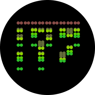 Python Script for Opentrons Artwork from opentrons import types import string metadata = { ‘protocolName’: ‘{Ashraful} - Opentrons Art - HTGAA’, ‘author’: ‘Ashraful’, ‘source’: ‘HTGAA 2026’, ‘apiLevel’: ‘2.20’ } Z_VALUE_AGAR = 2.0 POINT_SIZE = 0.75 sfgfp_points = [(-17.6,13.2), (-15.4,13.2), (-13.2,13.2), (-11,13.2), (-8.8,13.2), (11,13.2), (13.2,13.2), (15.4,13.2), (17.6,13.2), (-17.6,11), (-15.4,11), (-11,11), (-8.8,11), (8.8,11), (11,11), (13.2,11), (15.4,11), (17.6,11), (-15.4,8.8), (-13.2,8.8), (-8.8,8.8), (-6.6,8.8), (6.6,8.8), (8.8,8.8), (13.2,8.8), (15.4,8.8), (-13.2,6.6), (-11,6.6), (-6.6,6.6), (-4.4,6.6), (4.4,6.6), (6.6,6.6), (11,6.6), (13.2,6.6), (-11,4.4), (-8.8,4.4), (-4.4,4.4), (-2.2,4.4), (2.2,4.4), (4.4,4.4), (8.8,4.4), (11,4.4), (-8.8,2.2), (-6.6,2.2), (-2.2,2.2), (0,2.2), (2.2,2.2), (6.6,2.2), (8.8,2.2), (-6.6,0), (-4.4,0), (0,0), (4.4,0), (6.6,0), (-4.4,-2.2), (-2.2,-2.2), (0,-2.2), (2.2,-2.2), (4.4,-2.2), (-2.2,-4.4), (0,-4.4), (2.2,-4.4), (-2.2,-6.6), (0,-6.6), (2.2,-6.6), (-2.2,-8.8), (0,-8.8), (2.2,-8.8), (-2.2,-11), (0,-11), (2.2,-11), (-2.2,-13.2), (0,-13.2), (2.2,-13.2), (-11,-15.4), (-8.8,-15.4), (-6.6,-15.4), (-4.4,-15.4), (-2.2,-15.4), (0,-15.4), (2.2,-15.4), (4.4,-15.4), (6.6,-15.4), (8.8,-15.4), (11,-15.4), (13.2,-15.4), (-13.2,-17.6), (-11,-17.6), (-8.8,-17.6), (-6.6,-17.6), (-4.4,-17.6), (-2.2,-17.6), (0,-17.6), (2.2,-17.6), (4.4,-17.6), (6.6,-17.6), (8.8,-17.6), (11,-17.6), (13.2,-17.6), (15.4,-17.6), (-15.4,-19.8), (-13.2,-19.8), (-11,-19.8), (-8.8,-19.8), (-6.6,-19.8), (-4.4,-19.8), (-2.2,-19.8), (0,-19.8), (2.2,-19.8), (4.4,-19.8), (6.6,-19.8), (8.8,-19.8), (11,-19.8), (13.2,-19.8), (15.4,-19.8), (17.6,-19.8)] point_name_pairing = [(“sfgfp”, sfgfp_points)] # Robot deck setup constants TIP_RACK_DECK_SLOT = 9 COLORS_DECK_SLOT = 6 AGAR_DECK_SLOT = 5 PIPETTE_STARTING_TIP_WELL = ‘A1’ # Place the PCR tubes in this order well_colors = { ‘A1’: ‘sfGFP’, ‘A2’: ‘mRFP1’, ‘A3’: ‘mKO2’, ‘A4’: ‘Venus’, ‘A5’: ‘mKate2_TF’, ‘A6’: ‘Azurite’, ‘A7’: ‘mCerulean3’, ‘A8’: ‘mClover3’, ‘A9’: ‘mJuniper’, ‘A10’: ‘mTurquoise2’, ‘A11’: ‘mBanana’, ‘A12’: ‘mPlum’, ‘B1’: ‘Electra2’, ‘B2’: ‘mWasabi’, ‘B3’: ‘mScarlet_I’, ‘B4’: ‘mPapaya’, ‘B5’: ’eqFP578’, ‘B6’: ’tdTomato’, ‘B7’: ‘DsRed’, ‘B8’: ‘mKate2’, ‘B9’: ‘EGFP’, ‘B10’: ‘mRuby2’, ‘B11’: ‘TagBFP’, ‘B12’: ‘mChartreuse_TF’, ‘C1’: ‘mLychee_TF’, ‘C2’: ‘mTagBFP2’, ‘C3’: ‘mEGFP’, ‘C4’: ‘mNeonGreen’, ‘C5’: ‘mAzamiGreen’, ‘C6’: ‘mWatermelon’, ‘C7’: ‘avGFP’, ‘C8’: ‘mCitrine’, ‘C9’: ‘mVenus’, ‘C10’: ‘mCherry’, ‘C11’: ‘mHoneydew’, ‘C12’: ‘TagRFP’, ‘D1’: ‘mTFP1’, ‘D2’: ‘Ultramarine’, ‘D3’: ‘ZsGreen1’, ‘D4’: ‘mMiCy’, ‘D5’: ‘mStayGold2’, ‘D6’: ‘PA_GFP’ } # Mapping for visualization colors VISUALIZATION_COLOR_MAP = { ‘sfGFP’: ‘green’, ‘mRFP1’: ‘red’, ‘mKO2’: ‘orange’, ‘Venus’: ‘yellow’, ‘mKate2_TF’: ‘purple’, ‘Azurite’: ‘blue’, ‘mCerulean3’: ‘cyan’, ‘mClover3’: ’lightgreen’, ‘mJuniper’: ‘darkgreen’, ‘mTurquoise2’: ’teal’, ‘mBanana’: ‘gold’, ‘mPlum’: ‘plum’, ‘Electra2’: ’navy’, ‘mWasabi’: ’lime’, ‘mScarlet_I’: ‘darkred’, ‘mPapaya’: ‘peachpuff’, ’eqFP578’: ‘brown’, ’tdTomato’: ’tomato’, ‘DsRed’: ‘indianred’, ‘mKate2’: ‘darkmagenta’, ‘EGFP’: ‘chartreuse’, ‘mRuby2’: ‘firebrick’, ‘TagBFP’: ‘slateblue’, ‘mChartreuse_TF’: ‘darkseagreen’, ‘mLychee_TF’: ‘palevioletred’, ‘mTagBFP2’: ‘darkblue’, ‘mEGFP’: ’limegreen’, ‘mNeonGreen’: ’lawngreen’, ‘mAzamiGreen’: ‘mediumseagreen’, ‘mWatermelon’: ‘pink’, ‘avGFP’: ‘forestgreen’, ‘mCitrine’: ‘khaki’, ‘mVenus’: ‘olivedrab’, ‘mCherry’: ‘crimson’, ‘mHoneydew’: ‘honeydew’, # This will likely be too light ‘TagRFP’: ‘rosybrown’, ‘mTFP1’: ‘dodgerblue’, ‘Ultramarine’: ‘mediumblue’, ‘ZsGreen1’: ‘springgreen’, ‘mMiCy’: ‘peru’, ‘mStayGold2’: ‘goldenrod’, ‘PA_GFP’: ‘darkgreen’ } volume_used = { ‘sfgfp’: 0 } def update_volume_remaining(current_color, quantity_to_aspirate): rows = string.ascii_uppercase for well, color in list(well_colors.items()): if color == current_color: if (volume_used[current_color] + quantity_to_aspirate) > 250: # Move to next well horizontally by advancing row letter, keeping column number row = well[0] col = well[1:] # Find next row letter next_row = rows[rows.index(row) + 1] next_well = f"{next_row}{col}" del well_colors[well] well_colors[next_well] = current_color volume_used[current_color] = quantity_to_aspirate else: volume_used[current_color] += quantity_to_aspirate break def run(protocol): # Load labware, modules and pipettes protocol.home() # Tips tips_20ul = protocol.load_labware(‘opentrons_96_tiprack_20ul’, TIP_RACK_DECK_SLOT, ‘Opentrons 20uL Tips’) # Pipettes pipette_20ul = protocol.load_instrument(“p20_single_gen2”, “right”, [tips_20ul]) # Deep Well Plate temperature_plate = protocol.load_labware(’nest_96_wellplate_2ml_deep’, 6, ‘Deep Well Plate’) # Agar Plate agar_plate = protocol.load_labware(‘htgaa_agar_plate’, AGAR_DECK_SLOT, ‘Agar Plate’) agar_plate.set_offset(x=0.00, y=0.00, z=Z_VALUE_AGAR) # Get the top-center of the plate, make sure the plate was calibrated before running this center_location = agar_plate[‘A1’].top() pipette_20ul.starting_tip = tips_20ul.well(PIPETTE_STARTING_TIP_WELL) # Helper function (dispensing) def dispense_and_jog(pipette, volume, location): assert(isinstance(volume, (int, float))) # Go above the location above_location = location.move(types.Point(z=location.point.z + 2)) pipette.move_to(above_location) # Go downwards and dispense pipette.dispense(volume, location) # Go upwards to avoid smearing pipette.move_to(above_location) # Helper function (color location) def location_of_color(color_string): for well,color in well_colors.items(): if color.lower() == color_string.lower(): return temperature_plate[well] raise ValueError(f"No well found with color {color_string}") # Print pattern by iterating over lists for i, (current_color, point_list) in enumerate(point_name_pairing): # Skip the rest of the loop if the list is empty if not point_list: continue # Get the tip for this run, set the bacteria color, and the aspirate bacteria of choice pipette_20ul.pick_up_tip() max_aspirate = int(18 // POINT_SIZE) * POINT_SIZE quantity_to_aspirate = min(len(point_list)*POINT_SIZE, max_aspirate) update_volume_remaining(current_color, quantity_to_aspirate) pipette_20ul.aspirate(quantity_to_aspirate, location_of_color(current_color)) # Iterate over the current points list and dispense them, refilling along the way for i in range(len(point_list)): x, y = point_list[i] adjusted_location = center_location.move(types.Point(x, y)) dispense_and_jog(pipette_20ul, POINT_SIZE, adjusted_location) if pipette_20ul.current_volume == 0 and len(point_list[i+1:]) > 0: quantity_to_aspirate = min(len(point_list[i:])*POINT_SIZE, max_aspirate) update_volume_remaining(current_color, quantity_to_aspirate) pipette_20ul.aspirate(quantity_to_aspirate, location_of_color(current_color)) # Drop tip between each color pipette_20ul.drop_tip() Simulation # Execute Simulation / Visualization protocol = OpentronsMock(well_colors, VISUALIZATION_COLOR_MAP) run(protocol) protocol.visualize() Post-Lab Questions Find and describe a published paper that utilizes the Opentrons or an automation tool to achieve novel biological applications.
 Part A. Conceptual Questions How many molecules of amino acids do you take with a piece of 500 grams of meat? (on average an amino acid is ~100 Daltons) Skeletal muscle (meat) is approximately 20–25% protein by mass, with the remainder being water (~75%), fat, and connective tissue. Taking a conservative estimate of 20% protein, 500 g of meat contains roughly 100 g of protein. During digestion, proteases (pepsin in the stomach, trypsin and chymotrypsin in the small intestine) hydrolyse peptide bonds, releasing individual amino acids — the monomeric units. Using the given average amino acid molecular weight of 100 Daltons (100 g/mol): moles of amino acids = mass / molar mass = 100 g ÷ 100 g/mol = 1 mol Applying Avogadro’s number: N = 1 mol × 6.022 × 10²³ molecules/mol ≈ 6 × 10²³ molecules of amino acids This is a minimum estimate; the true figure is slightly higher because the average residue mass in a polypeptide chain is closer to 110–128 Da (due to the loss of water during peptide bond formation, the backbone residue mass averages ~110 Da, but free amino acids average ~128 Da). If we use 128 Da for free amino acids, we obtain ≈ 4.7 × 10²³ molecules — still on the order of half an Avogadro. Either way, the scale is strikingly close to 10²³, illustrating that a single meal-sized portion of protein delivers amino acids on the order of Avogadro’s number.
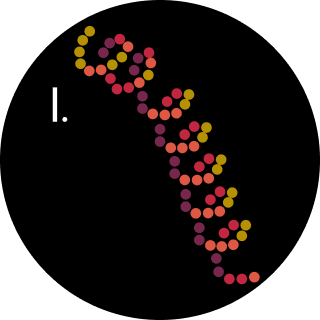 Part A: SOD1 Binder Peptide Design (From Pranam) Part 1: Generate Binders with PepMLM Begin by retrieving the human SOD1 sequence from UniProt (P00441) and introducing the A4V mutation. Using the PepMLM Colab linked from the HuggingFace PepMLM-650M model card: Generate four peptides of length 12 amino acids conditioned on the mutant SOD1 sequence. To your generated list, add the known SOD1-binding peptide FLYRWLPSRRGG for comparison. Record the perplexity scores that indicate PepMLM’s confidence in the binders
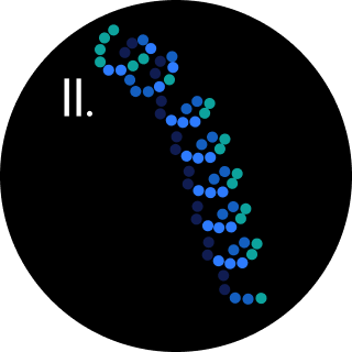 Assignment: DNA Assembly Answer these questions about the protocol in this week’s lab: What are some components in the Phusion High-Fidelity PCR Master Mix and what is their purpose? The Phusion High-Fidelity PCR Master Mix (NEB #M0531) is supplied as a convenient 2× pre-formulated reagent containing all reaction components except template DNA, primers, and water. Its key constituents and their functions are as follows. Phusion DNA Polymerase is the catalytic engine of the mix. It is a chimeric enzyme comprising a Pyrococcus-like thermostable polymerase core fused to a processivity-enhancing domain (derived from the Sso7d protein family), which allows the enzyme to remain bound to the DNA template for longer stretches and amplify fragments at higher speed and with greater fidelity than standard Taq polymerase. Crucially, Phusion carries a 3′→5′ proofreading exonuclease activity that removes incorrectly incorporated nucleotides, giving it an error rate more than 50-fold lower than Taq and roughly 6-fold lower than Pfu polymerase — making it the appropriate choice whenever sequence accuracy matters, such as for cloning (NEB, 2024). Deoxynucleotide triphosphates (dNTPs) — dATP, dCTP, dGTP, and dTTP — are the building blocks that the polymerase incorporates into the nascent DNA strand. They are pre-included in the master mix at a balanced concentration to minimise pipetting error. MgCl₂ (magnesium chloride) is an essential cofactor. Mg²⁺ ions coordinate with the phosphate groups of the incoming dNTP in the polymerase active site, enabling the phosphodiester bond-forming reaction. The concentration of free Mg²⁺ also influences polymerase processivity and primer–template specificity; the HF Buffer formulation has been optimised to include the appropriate Mg²⁺ concentration for standard templates. Reaction buffer (HF Buffer) maintains the correct pH and ionic strength for optimal polymerase activity. The buffer stabilises the enzyme during the high-temperature denaturation steps and helps establish reproducible annealing conditions. An alternative GC Buffer formulation is available for GC-rich or otherwise difficult templates, optionally supplemented with DMSO to reduce secondary structure in the template. Together, these components mean the researcher only needs to add template, primers, and water — dramatically reducing pipetting steps and the risk of component-level errors.
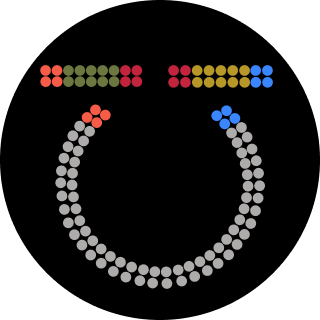 Assignment Part 1: Intracellular Artificial Neural Networks (IANNs) What advantages do IANNs have over traditional genetic circuits, whose input/output behaviors are Boolean functions? Traditional genetic circuits operate as Boolean logic gates: they classify inputs as either “on” (1) or “off” (0) and produce outputs that are likewise binary. While this is powerful for implementing discrete decisions — such as activating a kill switch if and only if two specific signals are simultaneously present — Boolean circuits are fundamentally limited in their ability to process the continuous, graded molecular signals that characterise real biological environments. Intracellular concentrations of transcription factors, metabolites, and signalling molecules are not naturally binary; they span continuous ranges that carry information that a simple Boolean threshold necessarily discards. IANNs overcome this limitation by implementing analog computation, in which each molecular “neuron” computes a weighted sum of its continuous-valued inputs, passes that sum through a nonlinear activation function, and produces a graded output that can itself serve as an input to the next layer. This architecture enables a single engineered cell to perform multi-threshold classification — distinguishing not just “signal present” from “signal absent” but grading responses proportionally to signal intensity, and separating input patterns that no Boolean gate could resolve without an exponentially larger circuit. For example, a cell expressing a two-input biomolecular perceptron can draw a separating hyperplane in the continuous input space of two molecular concentrations, classifying cell states that would require many cascaded Boolean gates to approximate. A second key advantage is graceful degradation under noise: because IANNs operate over a continuous input range, they can be designed with soft thresholds that smooth over stochastic fluctuations in molecule numbers — a pervasive problem in cells, where copy numbers of regulatory molecules are often in the tens to hundreds range. Boolean gates, which depend on crossing a hard threshold, are comparatively fragile to such noise. Third, IANNs are in principle extendable toward online learning, in which the synaptic weights (encoded by molecular concentrations or binding affinities) can be updated as a function of experience — an entirely alien concept to hardwired Boolean logic. Taken together, IANNs expand the computational vocabulary available to synthetic biology from a finite set of logic operations to a continuous, composable, and theoretically universal function approximation framework.
 Homework Part A: General and Lecturer-Specific Questions General homework questions 1. Explain the main advantages of cell-free protein synthesis over traditional in vivo methods, specifically in terms of flexibility and control over experimental variables. Name at least two cases where cell-free expression is more beneficial than cell production. Cell-free protein synthesis (CFPS) offers a fundamentally different operating logic from in vivo expression: because there is no living cell to maintain, the reaction environment is open and directly accessible to the experimenter. This openness translates into three practical advantages. First, reaction components — amino acid concentrations, buffer conditions, redox potential, template concentration — can be tuned independently and in real time without the buffering effects of cellular homeostasis. Second, toxic proteins that would kill or arrest growing cells can be expressed freely in CFPS, since there is no cell viability to protect. Third, non-canonical amino acids, isotopic labels, or synthetic chemical groups can be incorporated site-specifically by supplementing the reaction directly, enabling protein engineering strategies that are impossible to sustain through the protein expression machinery of a living cell. Two cases where cell-free expression is specifically more advantageous than cell-based production are: (1) membrane protein structural studies, where the absence of competing cellular membranes allows co-translational insertion directly into defined lipid nanodiscs of controlled composition, circumventing the protein aggregation and misfolding problems that arise during over-expression in intact cells; and (2) rapid on-demand diagnostic biosensors, where freeze-dried CFPS reactions can be deployed at the point of need without cold-chain infrastructure or biohazard containment — capabilities recently validated aboard the International Space Station.
 Part 1: Molecular Weight eGFP Sequence: VSKGEELFTG VVPILVELDG DVNGHKFSVS GEGEGDATYG KLTLKFICTT GKLPVPWPTL VTTLTYGVQC FSRYPDHMKQ HDFFKSAMPE GYVQERTIFF KDDGNYKTRA EVKFEGDTLV NRIELKGIDF KEDGNILGHK LEYNYNSHNV YIMADKQKNG IKVNFKIRHN IEDGSVQLAD HYQQNTPIGD GPVLLPDNHY LSTQSALSKD PNEKRDHMVL LEFVTAAGIT LGMDELYKLE HHHHHH Based only on the predicted amino acid sequence of eGFP (see below), what is the calculated molecular weight? You can use an online calculator like the one here: https://web.expasy.org/compute_pi/
 Part A: The 1,536 Pixel Artwork Canvas | Collective Artwork I missed the opportunity to contribute to the HTGAA CFPS bioart project. Later, I contributed to the SynBioBeta bioart project. I worked on part of the DNA on the center-left plate. What I liked: This kind of community-coordinated experiment builds genuine shared investment in the outcome, which is a rare and valuable pedagogical achievement. What could be improved: For future years, giving participants a low-resolution preview of the emerging canvas in near-real-time — without revealing the final image — would heighten the sense of collective emergence and encourage more strategic pixel placement.