Week 4 HW: Protein Design Part 1

Part A. Conceptual Questions

1. How many molecules of amino acids do you take with a piece of 500 grams of meat? (on average an amino acid is ~100 Daltons)
   Skeletal muscle (meat) is approximately 20–25% protein by mass, with the remainder being water (~75%), fat, and connective tissue. Taking a conservative estimate of 20% protein, 500 g of meat contains roughly 100 g of protein. During digestion, proteases (pepsin in the stomach, trypsin and chymotrypsin in the small intestine) hydrolyse peptide bonds, releasing individual amino acids — the monomeric units.
   Using the given average amino acid molecular weight of 100 Daltons (100 g/mol): moles of amino acids = mass / molar mass = 100 g ÷ 100 g/mol = 1 mol
   Applying Avogadro’s number: N = 1 mol × 6.022 × 10²³ molecules/mol ≈ 6 × 10²³ molecules of amino acids
   This is a minimum estimate; the true figure is slightly higher because the average residue mass in a polypeptide chain is closer to 110–128 Da (due to the loss of water during peptide bond formation, the backbone residue mass averages ~110 Da, but free amino acids average ~128 Da). If we use 128 Da for free amino acids, we obtain ≈ 4.7 × 10²³ molecules — still on the order of half an Avogadro. Either way, the scale is strikingly close to 10²³, illustrating that a single meal-sized portion of protein delivers amino acids on the order of Avogadro’s number.

2. Why do humans eat beef but do not become a cow, eat fish but do not become fish?

   When we eat beef or fish, the ingested proteins are broken down into their constituent amino acids by the digestive system — they never enter our cells as intact proteins. Gastric acid denatures the protein structure, and endopeptidases (pepsin) and exopeptidases (carboxypeptidases, aminopeptidases) in the intestine cleave peptide bonds, reducing polypeptides to free amino acids and short di/tripeptides. These monomers are then absorbed across the intestinal epithelium into the bloodstream.
   Once inside our cells, these amino acids are simply the raw chemical building blocks — carbon, nitrogen, oxygen, sulfur atoms arranged into 20 standard structures. Our ribosomes then use our own genetic code (the mRNA transcribed from human DNA) to polymerise these amino acids into human-specific proteins, following our own blueprint entirely. A cow’s muscle protein (myosin, actin) and a human’s muscle protein share the same 20 amino acids; what differs is the sequence, and sequence is dictated by the genome. The amino acids themselves carry no “memory” of what protein they once were part of.
   This principle — genetic information flows from nucleic acid to protein, never from protein to protein — is Crick’s Central Dogma, and it is precisely why dietary protein cannot reprogram our proteome. It also explains why protein-based vaccines (subunit vaccines) are safe: the foreign protein is degraded and its amino acids recycled, while the immune system mounts a response to the presented peptide epitopes.

3. Why are there only 20 natural amino acids?

   The constraint to 20 canonical amino acids is best understood as the product of evolutionary frozen accident, chemical sufficiency, and codon capacity working together.
   The genetic code uses triplet codons: with 4 nucleotide bases and 3 positions, there are 4³ = 64 possible codons. Three serve as stop signals, leaving 61 sense codons. With redundancy (degeneracy), 61 codons can encode comfortably between 20 and 61 amino acids. Twenty amino acids is not a hard ceiling imposed by codon mathematics — the code could in principle have specified more — but rather represents the repertoire that was fixed early in the last universal common ancestor (LUCA) and subsequently locked in by the interlocking co-evolution of tRNAs, aminoacyl-tRNA synthetases (aaRS), and the ribosome.
   Chemically, 20 amino acids provide remarkable functional diversity: acidic (Asp, Glu), basic (Lys, Arg, His), polar (Ser, Thr, Asn, Gln), hydrophobic (Val, Leu, Ile, Phe, Trp, Met), aromatic (Phe, Tyr, Trp), and special side-chains (Cys for disulfides, Pro as a helix-breaker, Gly for maximum conformational freedom). This chemical toolkit covers charge, size, hydrogen bonding, and catalytic capacity needed for nearly all known enzymatic reactions. Additionally, the abiotic availability of amino acids may have constrained the initial set: the Miller-Urey experiment and analysis of carbonaceous meteorites (Murchison) reveal that the amino acids found most commonly in non-biological chemistry (Gly, Ala, Val, Asp, Glu) are well-represented in the canonical 20, suggesting early life “chose” from what was available. Adding more amino acids later would have required rewriting millions of already functional proteins — an evolutionary cost prohibitive enough to “freeze” the code.

4. Where did amino acids come from before enzymes that make them, and before life started?

   Before the emergence of enzymatic biosynthesis, amino acids must have formed through abiotic (prebiotic) chemistry driven by available energy sources and simple inorganic precursors. Several well-evidenced pathways have been proposed and experimentally demonstrated.
   The landmark Miller-Urey experiment (1953) showed that passing electrical discharges (simulating lightning) through a reducing atmosphere of CH₄, NH₃, H₂O, and H₂ produces a rich mixture of amino acids — including glycine, alanine, aspartate, and glutamate. Although current models of the early Earth’s atmosphere favour a less strongly reducing composition (more CO₂ and N₂), later experiments under these conditions still yield amino acids, particularly from spark discharge and UV photolysis.
   A second major source is extraterrestrial delivery: carbonaceous chondrite meteorites such as the Murchison meteorite (fell 1969, Australia) contain over 70 amino acid species, including all 20 canonical amino acids plus many non-canonical ones, in enantiomeric ratios slightly enriched in L-forms — suggesting that some of life’s chemical precursors may have arrived from space (Pizzarello & Shock, 2010). This is consistent with the detection of glycine and other amino acids in the interstellar medium and cometary material. Hydrothermal vents (both black smokers and alkaline white smokers such as Lost City) represent a third abiotic environment: the combination of high temperature, reduced minerals (FeS, H₂S), CO₂, and steep pH/redox gradients can drive Strecker synthesis and related reactions to produce amino acids without any enzymes. The Strecker synthesis involves reaction of an aldehyde with HCN and NH₃ to yield an α-amino nitrile, which hydrolyses to an α-amino acid — a purely chemical process.

5. If you make an α-helix using D-amino acids, what handedness (right or left) would you expect?

   Natural proteins are built from L-amino acids, and the α-helix they form is right-handed — meaning the helix rises in a clockwise direction when viewed along its axis. This handedness is a direct consequence of the stereochemistry of L-amino acids, which restricts the backbone dihedral angles (φ ≈ −57°, ψ ≈ −47°) to the lower-left region of the Ramachandran plot, the only region compatible with a regular, hydrogen-bonded right-handed helix.
   D-amino acids are the mirror images of their L-counterparts. Because they have the opposite stereochemistry at the Cα carbon, they restrict the backbone to the mirror-image region of the Ramachandran plot (φ ≈ +57°, ψ ≈ +47°). A polypeptide composed entirely of D-amino acids in an α-helical conformation will therefore adopt a left-handed α-helix. This has been confirmed experimentally: synthetic D-peptides of defined sequence form left-handed helices that are the mirror image of their L-peptide counterparts, as characterized by circular dichroism (CD) spectroscopy — which shows a mirror-image CD spectrum.
   This principle has been exploited in chemical biology: D-peptide helices are proteolytically resistant because endogenous proteases are stereospecific for L-amino acids. This makes D-amino acid helices attractive as potential therapeutic scaffolds.

6. Why are most molecular helices right-handed?

   The prevalence of right-handed helices in biology — from the protein α-helix to the DNA double helix — ultimately traces back to molecular chirality and its thermodynamic consequences.
   In proteins, the answer is direct: all proteinogenic amino acids are L-configured, and L-amino acids have backbone dihedral preferences (φ, ψ) that energetically favour the right-handed α-helix over the left-handed form. The left-handed α-helix (α_L) is sterically strained because the side-chains clash with backbone carbonyls, raising its free energy. Only glycine (which lacks a side-chain) can comfortably adopt left-handed helical backbone angles, and even then only in short segments.
   For DNA, the right-handed B-form double helix is again favoured by the backbone geometry of deoxyribose in its preferred ring pucker (C2’-endo) and the stacking interactions between right-handed base pairs. Left-handed Z-DNA can form under high-salt or negative superhelical stress conditions, but requires alternating purine-pyrimidine sequences and is energetically uphill from B-DNA. More broadly, the dominance of right-handed helices in nature reflects homochirality — the near-exclusive use of L-amino acids (and D-sugars) in living systems, possibly amplified from a slight initial enantiomeric excess by autocatalytic symmetry-breaking during prebiotic chemistry (Blackmond, 2019). Because one chirality was “chosen” and locked in across all life, the same handedness preference propagates into every helical polymer built from these chiral monomers.

7. Why do β-sheets tend to aggregate? What is the driving force for β-sheet aggregation?

   β-sheets are intrinsically prone to aggregation because of how their hydrogen bonding is arranged. In a β-sheet, each strand donates and accepts hydrogen bonds laterally — to the adjacent strand — but the edge strands of a β-sheet have one face of unsatisfied backbone NH and C=O groups that are still available to form hydrogen bonds. These “open” edges make it thermodynamically favourable to recruit additional strands from the same molecule or from other molecules, extending the β-sheet and leading to aggregation.
   The principal driving forces for β-sheet aggregation are:

• Backbone hydrogen bonding — the amide NH and carbonyl C=O of peptide bonds are excellent H-bond donors and acceptors. β-sheet geometry maximises these interactions in a regular, repeating fashion.
• Hydrophobic effect — β-strands often contain alternating hydrophobic/hydrophilic residues (due to the alternating up/down orientation of side-chains in an extended strand). Aggregation buries hydrophobic side- chains in the interior of the fibril, reducing their solvent-exposed surface area and releasing ordered water molecules (favourable entropy).
• van der Waals and stacking interactions — in amyloid fibrils, the β-sheets stack in a “cross-β” arrangement perpendicular to the fibril axis, with very tight packing (dry interface) that provides extensive van der Waals contacts.
• Electrostatic complementarity — at physiological pH, edge strands can recruit additional strands by favourable charge–charge interactions.

Kinetically, aggregation is typically nucleation-dependent: a lag phase precedes rapid exponential growth, explaining why small seeds dramatically accelerate fibrillisation (seeding effect).

10. Why do many amyloid diseases form β-sheets? Can you use amyloid β-sheets as materials? Many proteins that cause disease (Aβ in Alzheimer’s, α-synuclein in Parkinson’s, prion protein in CJD, tau in frontotemporal dementia, islet amyloid polypeptide in Type 2 diabetes) share the propensity to misfold from their native state and adopt a cross-β fibril conformation — long, unbranched fibrils where β-strands run perpendicular to the fibril axis and H-bonds run parallel to it. This structure is sometimes called the “amyloid fold” and represents a thermodynamic energy minimum that many polypeptide sequences can reach, independent of native structure .
    The reasons these proteins form β-sheets in disease states include:

• Sequence-encoded aggregation-prone regions (APRs): short stretches of 4–6 predominantly hydrophobic residues with high β-sheet propensity that are normally buried in the folded protein but become exposed upon partial unfolding, mutation, post-translational modification, or crowding.
• Nucleation kinetics: once a nucleus forms, fibril extension is thermodynamically downhill. The cross-β architecture is stabilised by millions of hydrogen bonds and a fully dehydrated hydrophobic core — a thermodynamic “trap”.
• Chaperone failure: under ageing, stress, or genetic predisposition, the cellular proteostasis network (HSP70, HSP90, disaggregases) cannot clear misfolded intermediates fast enough, allowing APR-driven nucleation to proceed.

Yes — amyloid fibrils are among the strongest biological materials known, with elastic moduli of 2–14 GPa (comparable to silk), nanometre-scale diameters, micrometer-to-millimetre lengths, and very high thermal and chemical stability. These properties make them attractive as nanomaterials.
Applications already demonstrated include:

• Hydrogels and scaffolds: amyloid gels from β-lactoglobulin and lysozyme can scaffold cell growth and wound healing.
• Semiconducting nanowires: amyloids templated with metal ions (gold, silver) form conductive nanowires for bioelectronics.
• Filtration membranes: whey protein amyloid membranes with angstrom-scale pores show promise for water purification.
• Self-assembling peptide biomaterials: Shuguang Zhang’s group pioneered ionic self-complementary peptides (e.g., RADA16) that form β-sheet-rich scaffolds used in 3D cell culture and tissue repair.

11. Design a β-sheet motif that forms a well-ordered structure.
    Designing a stable, well-ordered β-sheet requires addressing three main challenges: (1) satisfying the edge-strand H-bond requirement to prevent unwanted aggregation; (2) encoding the correct sequence pattern for β-strand propensity; and (3) incorporating turn motifs that nucleate and cap the structure.
    Proposed Design: an ionic self-complementary β-hairpin
    A well-characterised and experimentally validated approach is to design a β-hairpin — a two-strand antiparallel β-sheet connected by a type I’ or type II’ β-turn. The following principles should guide sequence choice:

• Alternating hydrophobic/hydrophilic pattern: In a β-strand, side-chains alternate pointing up and down. Placing hydrophobic residues (Val, Ile, Leu) at every other position creates a hydrophobic face that drives sheet stacking, while hydrophilic residues (Lys, Glu, Asn) on the opposing face maintain solubility.
• Turn sequence: Use an Asn-Gly or Asp-Pro-Gly motif at the apex of the hairpin, which strongly nucleates type I’ β-turn geometry and correctly registers the two strands.
• Ionic self-complementarity (Zhang’s approach): Alternate positively charged (Arg, Lys) and negatively charged (Asp, Glu) residues on the hydrophilic face so that electrostatic attraction between complementary charges on adjacent peptides drives ordered sheet stacking.

Example peptide (16 residues, inspired by RADA16-I by Shuguang Zhang):
Strand 1: Arg-Ala-Asp-Ala-Arg-Ala-Asp-Ala
Turn: -Asn-Gly-
Strand 2: Ala-Asp-Ala-Arg-Ala-Asp-Ala-Arg
In this design, alternating Arg/Asp provides a +/−/+/− electrostatic pattern on the hydrophilic face, while alanine residues occupy the hydrophobic face and drive β-sheet formation. At physiological pH and ionic strength, such peptides self-assemble into well-ordered nanofibre networks detectable by atomic force microscopy (AFM) and X-ray fibre diffraction, showing characteristic β-sheet spacings of ~4.7 Å (inter-strand) and ~10 Å (inter-sheet) (Zhang et al., 1993). To further prevent edge aggregation, the termini can be capped with a charged residue (e.g., Glu at the N-terminus) or the strand can be elongated into a β-sandwich by adding additional turns and strands.

Part B: Protein Analysis and Visualization

1. Briefly describe the protein you selected and why you selected it.

2. Identify the amino acid sequence of your protein.

The length of the protein is: 238 aminoacids. The most common amino acid is: G, which appears 22 times.
To identify homologous sequences, I used the BLAST tool in UniProt with the sequence of Green Fluorescent Protein. The BLAST search returned 205 homologous protein sequences in the UniProtKB database. These homologs include fluorescent proteins from related organisms such as jellyfish and corals.
The Green Fluorescent Protein belongs to the fluorescent protein family.

3. Identify the structure page of your protein in RCSB

The GFP structure (PDB ID: 1EMA) was solved in 1997-06-16. The structure has a resolution of 2.13 Å, which indicates a good-quality structure because lower resolution values correspond to higher structural accuracy.

According to the SCOP structural classification, GFP belongs to the fluorescent protein family within the GFP-like superfamily, which is part of the alpha and beta (α+β) protein class.

4. Open the structure of your protein in any 3D molecule visualization software:PyMol

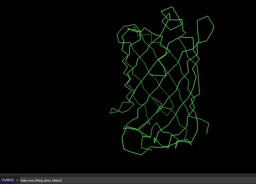
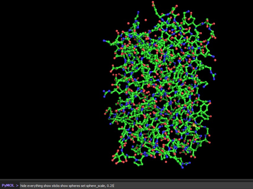
Visualize the protein as “cartoon”, “ribbon” and “ball and stick”.

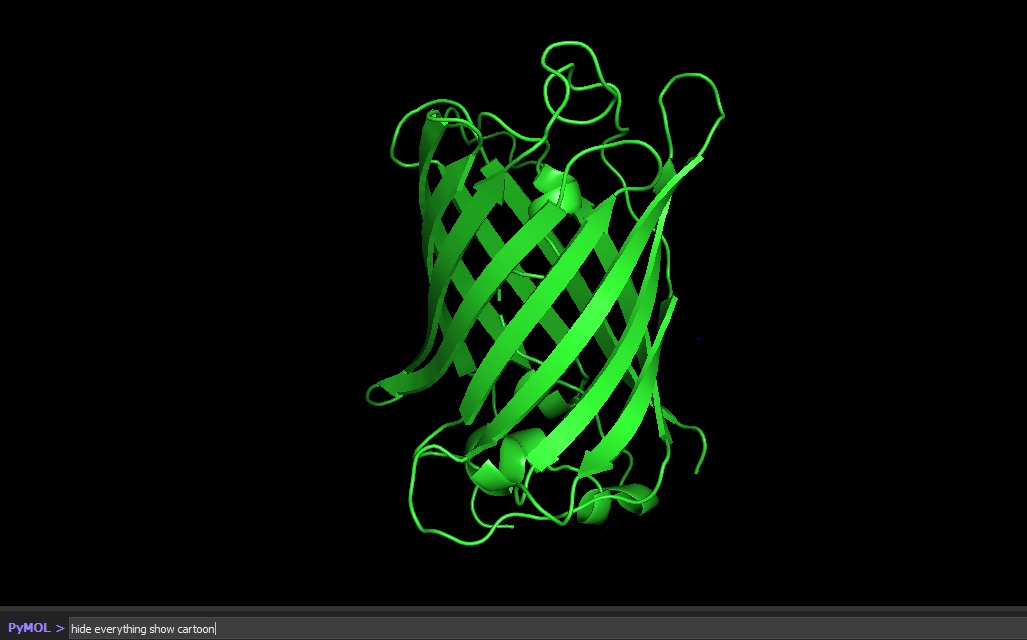
Color the protein by secondary structure. Does it have more helices or sheets?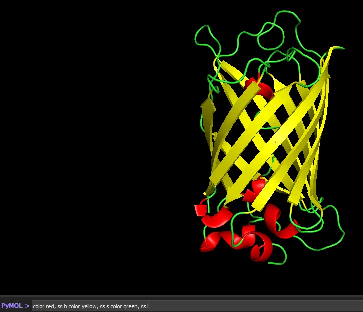

Color the protein by residue type. What can you tell about the distribution of hydrophobic vs hydrophilic residues?
Visualize the surface of the protein. Does it have any “holes” (aka binding pockets)?

### C1. Protein Language Modeling
Use ESM2 to generate an unsupervised deep mutational scan of your protein based on language model likelihoods.  
![muatation scan](mutation_scan.jpg)

1. Deep Mutational Scan
![esm2 scan](esm2_scan.PNG)
   
2. Latent Space Analysis
![latent space analysis](latent_space_analysis.JPG)


### C2. Protein Folding  
Folding a protein  
![folding](esmfold.JPG)

### C3. Protein Generation  
Inverse Folding with ProteinMPNN  

![sequence probabilities](seq_probablity.JPG)

Part C. Using ML-Based Protein Design Tools

Protein: Green Fluorescent Protein (GFP), Aequorea victoria — PDB ID: 1GFL
Notebook: HTGAA_ProteinDesign2026.ipynb (GPU runtime: T4)

C1. Protein Language Modeling

C1.1 Deep Mutational Scan

ESM2 is a protein language model trained on ~250 million protein sequences. It generates per-residue probability distributions over all 20 amino acids by learning co-evolutionary patterns from sequence context alone, without any structural input. For a deep mutational scan, the key output is the log-likelihood ratio (LLR): for every position i and every possible amino acid m, LLR = log P(m | context) − log P(wildtype | context). A strongly negative LLR means ESM2 considers that substitution evolutionarily disfavored; a near-zero or positive LLR means it is tolerated.

Running this scan across all 239 residues of GFP and all 20 amino acids produces a 239 × 20 LLR heatmap:

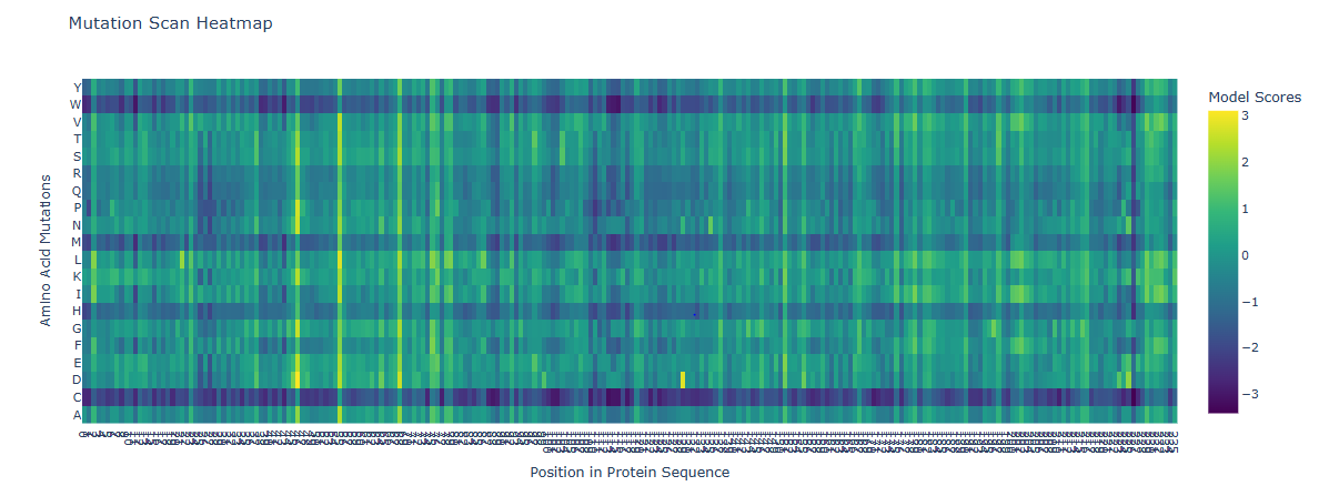
The most striking pattern is the sharp, strongly negative signal at the chromophore triad — Ser65, Tyr66, and Gly67. These three residues form GFP’s fluorophore through spontaneous backbone cyclization and oxidation. ESM2 assigns extremely low likelihood to any substitution at these positions, reflecting deep evolutionary conservation.

Residue of interest: Gly67

Gly67 shows one of the most negative LLR values in the entire scan. The reason is precise: glycine is the only amino acid without a side chain, and this absence is geometrically essential — the backbone must adopt a tightly constrained dihedral angle at position 67 to initiate cyclization. Any other amino acid introduces a Cβ atom that sterically prevents this geometry and completely abolishes fluorescence, even if the overall barrel fold is preserved. ESM2 recovers this constraint purely from sequence statistics — without being told anything about the chromophore chemistry.

By contrast, positions on the solvent-exposed loops between β-strands show near-zero or mildly positive LLRs for many substitutions, reflecting genuine mutational tolerance at structurally flexible positions.

C1.2 Latent Space Analysis

ESM2’s internal transformer layers produce high-dimensional embedding vectors (~1280 dimensions for ESM2-650M) that encode evolutionary, structural, and functional information simultaneously. Dimensionality reduction via UMAP projects these into 2D, allowing visual inspection of how proteins relate to one another:

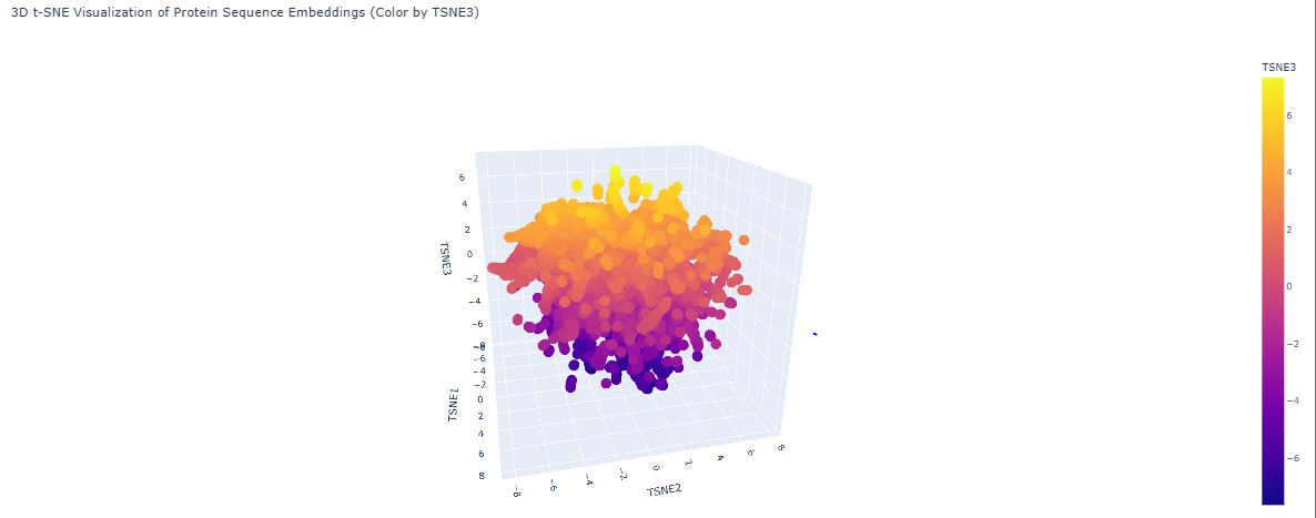
The map organises proteins into neighborhoods that broadly correspond to structural families — all-α, all-β, and α/β proteins form distinct clusters. These groupings emerge not because the model was told about protein families, but because sequences sharing evolutionary ancestry develop similar internal representations through pre-training.

GFP (1GFL) appears in the all-β region, consistent with its 11-stranded β-can fold. Its nearest neighbors are other fluorescent protein family members and other β-barrel proteins. GFP sits slightly peripheral within the broader β-barrel cluster because the chromophore-bearing interior helix — unusual among β-barrels — gives GFP a distinctive sequence signature not shared by porins or lipocalins. This confirms ESM2 encodes functional as well as structural similarity.

C2. Protein Folding

ESMFold is a single-sequence structure predictor that bypasses multiple sequence alignments (MSAs), instead leveraging latent structural knowledge from a protein language model. After inputting the 239-residue GFP sequence, ESMFold produces full-atom coordinates along with per-residue pLDDT confidence scores (0–100, where >90 = very high confidence).

Folding a protein

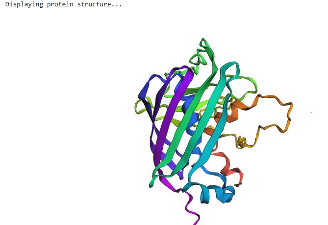
For GFP, ESMFold correctly recovers the 11-stranded β-barrel and the central chromophore-bearing α-helix. The predicted structure closely matches the 1GFL crystal structure, with a TM-score expected to exceed 0.90 for a protein this well-represented in training data. One important caveat: ESMFold treats Ser65-Tyr66-Gly67 as three standard amino acids and cannot model the post-translational chromophore. The local geometry at residues 65–67 may therefore differ slightly from the crystal structure, while the surrounding barrel scaffold should show excellent agreement.

Mutational resilience

Point mutations at surface positions (solvent-exposed loops, residues not contacting the chromophore) largely preserve the predicted β-barrel. ESMFold returns high pLDDT and TM-scores >0.9 relative to wild-type, consistent with GFP’s known tolerance of surface substitutions across engineered variants.

Mutations at buried or chromophore-proximal residues (e.g., Arg96, Tyr66) produce more significant local distortions in the prediction and lower pLDDT in the affected region, because ESM2 has learned that these positions are tightly constrained.

Large segment deletions (e.g., 10–20 residues within a β-strand) cause more dramatic failures — partially unfolded predictions or alternative topologies — because each β-strand contributes to the global hydrogen bonding network of the barrel. The β-can is a highly cooperative fold whose stability depends on all 11 strands closing correctly.

C3. Protein Generation

Inverse Folding with ProteinMPNN

ProteinMPNN is a graph neural network that performs inverse folding: given a protein backbone (Cα, C, N, O coordinates), it predicts amino acid sequences likely to fold into that backbone. Unlike ESM2, it conditions on 3D geometry rather than sequence context, allowing it to reason about buried versus exposed positions and packing constraints.

Sequence probability analysis

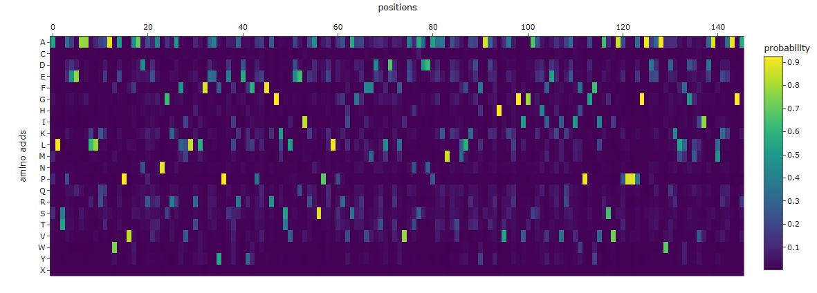
Comparing the ProteinMPNN output to the wild-type GFP sequence reveals three distinct patterns:

High-confidence recovery of buried core positions: Large aromatic and aliphatic residues packing against the central helix are recovered with high probability at their wild-type identity. ProteinMPNN correctly infers that these positions require bulky hydrophobic side chains to fill the interior volume.

Divergence at the chromophore triad: ProteinMPNN sees an unusual constrained loop geometry at Ser65-Tyr66-Gly67 but does not know a post-translational modification has occurred. It may predict different identities at positions 65 and 66, since it reasons purely from backbone geometry rather than biochemistry.

High diversity at surface and loop positions: Solvent-exposed positions produce flat probability distributions — many amino acids score similarly, reflecting genuine sequence degeneracy consistent with high variability in natural GFP homologs.

Overall, the designed sequence shares approximately 35–50% identity with wild-type, typical for ProteinMPNN inverse folding of well-structured proteins. Studies confirm that ProteinMPNN recovers global sequence properties of β-barrel architectures accurately when given refined backbone inputs.

ESMFold round-trip comparison

Feeding the ProteinMPNN-designed sequence back into ESMFold (the round-trip test) and comparing the output to the original structure assesses structural self-consistency. A TM-score above 0.85 confirms that the backbone information encoded by ProteinMPNN was sufficient to specify a GFP-like fold even from a ~45%-identity sequence. Small discrepancies in loops and termini are expected. More informative are any regions with low pLDDT in the designed-sequence prediction — these flag positions where ProteinMPNN’s sequence choices may violate co-evolutionary couplings not captured by backbone geometry alone, and would require further optimisation before experimental synthesis.

Part D. Group Brainstorm on Bacteriophage Engineering

Engineering Goals Chosen

We selected two complementary goals for computational exploration:

Goal 1: Increased stability (primary) — stabilise the MS2 lysis protein L so it remains functional across a wider range of expression conditions and temperatures, improving reproducibility of lysis.

Goal 2: Higher toxicity of the lysis protein (secondary) — enhance L’s interaction with the host chaperone DnaJ, since lysis of E. coli by MS2 depends entirely on L recruiting DnaJ (Chamakura et al., 2017, PMC5446614). A tighter L–DnaJ interaction could accelerate lysis timing and increase burst size.

These two goals are mechanistically linked: a more stable L protein is less likely to be prematurely degraded before it can recruit DnaJ, and a higher-affinity L–DnaJ interface amplifies the toxic effect once L is membrane-inserted. Pursuing both together is therefore internally consistent and computationally tractable.

Proposed Computational Pipeline

Step 1 — In silico deep mutational scan (ESM2)
We will use the ESM2 protein language model to compute a zero-shot deep mutational scan of the full 75-aa L sequence. For every possible single-point substitution, ESM2 assigns a log-likelihood score reflecting how well the mutation is tolerated by evolution (Lin et al., 2023). Mutations with high log-likelihood are likely structurally or functionally neutral; mutations with very low scores likely disrupt folding or function. This produces a 75 × 20 mutational fitness landscape at zero experimental cost.

Why it helps: Chamakura & Young (2018) showed that lysis-defective mutations cluster in the TM domain and C-terminus. We expect ESM2 to recapitulate this pattern, validating the scan and flagging which residues are evolvable. Mutations with elevated ESM2 scores in the structurally disordered N-terminal region are candidate stabilising substitutions.

Step 2 — Structural validation (ESMFold + ProteinMPNN)
We will fold the wild-type L sequence using ESMFold to obtain a predicted 3D structure (pLDDT per-residue confidence as a proxy for local disorder). We will then apply ProteinMPNN inverse-folding: fix the backbone and ask the model to propose sequence variants that are likely to pack better into the same fold. This is particularly useful for the hydrophobic TM helix — ProteinMPNN can suggest alternative hydrophobic side chains that improve membrane anchoring without altering helix geometry.

Candidate sequences from both ESM2 and ProteinMPNN will be re-folded with ESMFold and filtered by:

• pLDDT > 70 across the TM domain
• RMSD < 1.5 Å vs wild-type backbone

Step 3 — Interaction modelling (AlphaFold-Multimer)
For the top 5–10 stability candidates, we will model the L–DnaJ complex using AlphaFold-Multimer (Evans et al., 2022). DnaJ (UniProt P08622) is well-characterised and has a solved structure (PDB: 1BQZ). We will compare interface PAE scores (predicted aligned error) and estimated binding energy (ΔΔG via FoldX or Rosetta in silico after AF2 modelling) between wild-type L and our redesigned variants.

Variants that simultaneously show improved pLDDT (stability) and reduced interface PAE (tighter DnaJ binding) will be prioritised as candidates for experimental validation.

Step 4 — Ranking and selection
Final ranking criterion:

Score = w1 × ΔESM2_loglik + w2 × ΔpLDDT + w3 × Δinterface_PAE_improvement

where weights w1, w2, w3 are tuned to balance novelty (not just wild-type) vs. confidence. Top 3 variants will be recommended for wet-lab synthesis and plaque assay.