Ashraful — HTGAA Spring 2026

About me
Hi! I’m Ashraful, currently a fourth-year undergraduate student in Plant Biology at the University of Dhaka, Bangladesh. I am passionate about: Plant synthetic biology , Biosecurity & Agentic AI.
Hi! I’m Ashraful, currently a fourth-year undergraduate student in Plant Biology at the University of Dhaka, Bangladesh. I am passionate about: Plant synthetic biology , Biosecurity & Agentic AI.


  </div>
</div>
<div class="card-image">
    <img src="/2026a/md-ashraful-islam/homework/week-01-hw-principles-and-practices/week1icon-pipette.featured.png">
</div>
1. First, describe a biological engineering application or tool you want to develop and why.
I want to develop a plant stress-responsive synthetic gene circuit in a chloroplast-derived cell-free system that detects stress signals like pathogen RNA or heavy metals and produces a visible reporter output. This tool enables rapid, safe prototyping of plant gene circuits and allows assessment of biosecurity risks, such as misfires or misuse, without using live plants. The primary motivation for this project is to build upon and extend the work of the 2021 iGEM Marburg team, leveraging their foundational advances to develop more responsive and secure plant synthetic biology tools.
2. Next, describe one or more governance/policy goals related to ensuring that this application or tool contributes to an “ethical” future, like ensuring non-malfeasance (preventing harm). Break big goals down into two or more specific sub-goals.
Goal: Ensure safe and responsible use of plant stress-responsive synthetic gene circuits.
Sub-goals: Prevent misuse or accidental harm using logic gates, kill switches, and monitoring protocols. Promote constructive applications for crop protection and biosecurity preparedness. Maintain transparency and accountability through documentation and ethical guidelines.
3. Next, describe at least three different potential governance “actions” by considering the four aspects below (Purpose, Design, Assumptions, Risks of Failure & “Success”): 1. Purpose: 2. Design: 3. Assumptions: 4. Risks of Failure & “Success”:
| Action | Purpose | Design | Assumptions | Risks of Failure & Success |
|---|---|---|---|---|
| 1. Circuit Safeguards | Require logic gates, kill switches, self-limiting designs | Researchers design safeguards; regulators certify | Safeguards reliably prevent harm | Failure: safeguards bypassed or misconfigured; Success: false sense of security reduces oversight |
| 2. Pre-Deployment Risk Assessment | Mandatory biosecurity assessment before field use | Researchers submit risk reports; regulators approve | Risks can be anticipated and mitigated | Failure: assessments become superficial; Success: bureaucratic compliance slows innovation |
| 3. Incentive-Based Governance & Responsible-Use Norms | Promote safe, transparent, and ethical plant synbio use | Funders require safety plans, audits, and training | Incentives motivate responsible behavior | Failure: voluntary uptake limits coverage; Success: norms diffuse unevenly across actors |
4. Next, score (from 1-3, with 1 as the best, or n/a) each of your governance actions against your rubric of policy goals. The following is one framework but feel free to make your own:
| Does the option: | Option 1: Circuit Safeguards | Option 2: Pre-Deployment Risk Assessment | Option 3: Incentive-Based Governance & Responsible-Use Norms |
|---|---|---|---|
| Enhance Biosecurity | |||
| • By preventing incidents | 1 | 2 | 3 |
| • By helping respond | 2 | 1 | 2 |
| Foster Lab Safety | |||
| • By preventing incidents | 1 | 2 | 2 |
| • By helping respond | 2 | 1 | 2 |
| Protect the environment | |||
| • By preventing incidents | 1 | 2 | 2 |
| • By helping respond | 2 | 1 | 3 |
| Other considerations | |||
| • Minimizing costs/burdens | 2 | 3 | 1 |
| • Feasibility | 1 | 2 | 1 |
| • Does not impede research | 2 | 3 | 1 |
| • Promote constructive applications | 2 | 2 | 1 |
5. Last, drawing upon this scoring, describe which governance option, or combination of options, you would prioritize, and why. Outline any trade-offs you considered as well as assumptions and uncertainties.
Based on the scoring, I prioritize a combined approach led by Option 1 (Circuit Safeguards) and Option 3 (Incentive-Based Governance & Responsible-Use Norms), with Option 2 (Pre-Deployment Risk Assessment) applied selectively to higher-risk projects. Circuit safeguards are most effective at preventing incidents by embedding safety directly into design, while incentive-based governance best preserves feasibility, equity, and research freedom. Risk assessments are valuable for response and preparedness, but can impose high burdens if universally required. Key trade-offs involve balancing prevention with flexibility. Ethical concerns include overreliance on technical fixes and inequitable access; tiered governance and ongoing safety education help address these risks.
Nature’s machinery for copying DNA is called polymerase. What is the error rate of polymerase? How does this compare to the length of the human genome. How does biology deal with that discrepancy?
The error rate of the polymerase is 1 in 10⁶ bases. The human genome is approximately 3 × 10⁹ base pairs long. Therefore, when compared to the length of the human genome, this error rate corresponds to about 3 × 10³ errors per genome. Biology deals with this discrepency by proofreading, mismatch repair (MMR) system, & redundancy and selection.
How many different ways are there to code (DNA nucleotide code) for an average human protein? In practice what are some of the reasons that all of these different codes don’t work to code for the protein of interest?
The number of different DNA sequences (theoretical): ~3⁴⁰⁰ ≈ 10¹⁹⁰ for a 400-amino-acid protein. Many DNA sequences don’t work in practice due to codon usage bias, mRNA structure, protein folding dynamics, regulatory elements, and mutation robustness/cellular context.
What’s the most commonly used method for oligo synthesis currently?
Phosphoramidite (solid‑phase) chemistry.
Why is it difficult to make oligos longer than 200nt via direct synthesis?
Per‑cycle inefficiencies and side reactions cause the full‑length fraction to fall rapidly with length.
The cumulative yield of full‑length product becomes essentially zero; chemical synthesis is not scalable to kilobase lengths.
Ten amino acids commonly treated as essential for animals: Lysine; Methionine; Tryptophan; Threonine; Valine; Isoleucine; Leucine; Arginine; Histidine; Phenylalanine. Lysine auxotrophy is a useful mitigation but not a reliable sole safeguard —it can be rescued by environmental lysine, cross‑feeding, or genetic escape, so treat it as one layer in a multi‑layered containment strategy.
(For completing the second part of the homework (Week 2 preparation), I verified my answers and summarized the lecture slides to clarify specific points, using ChatGPT as a support tool.)
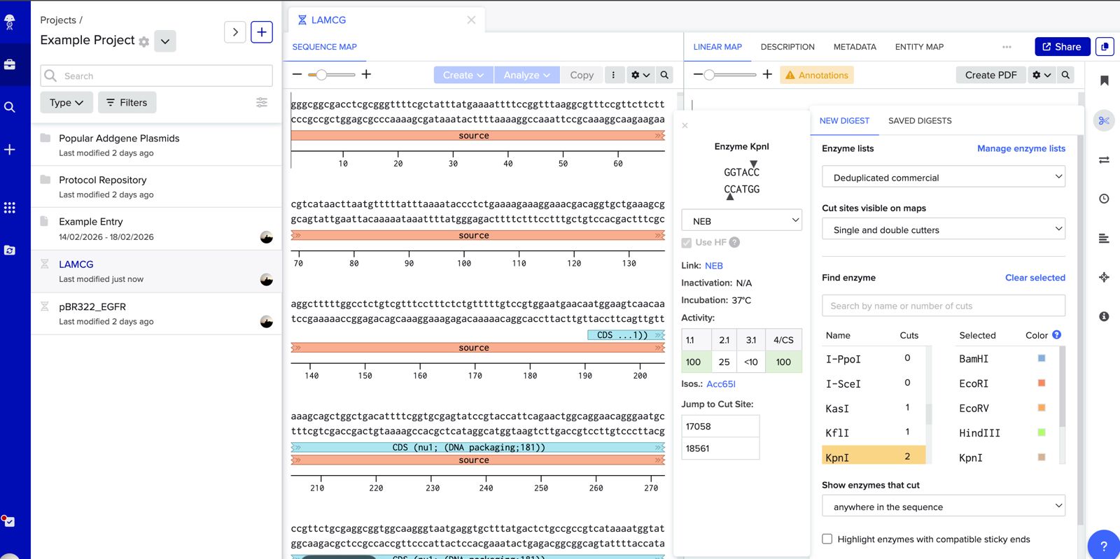
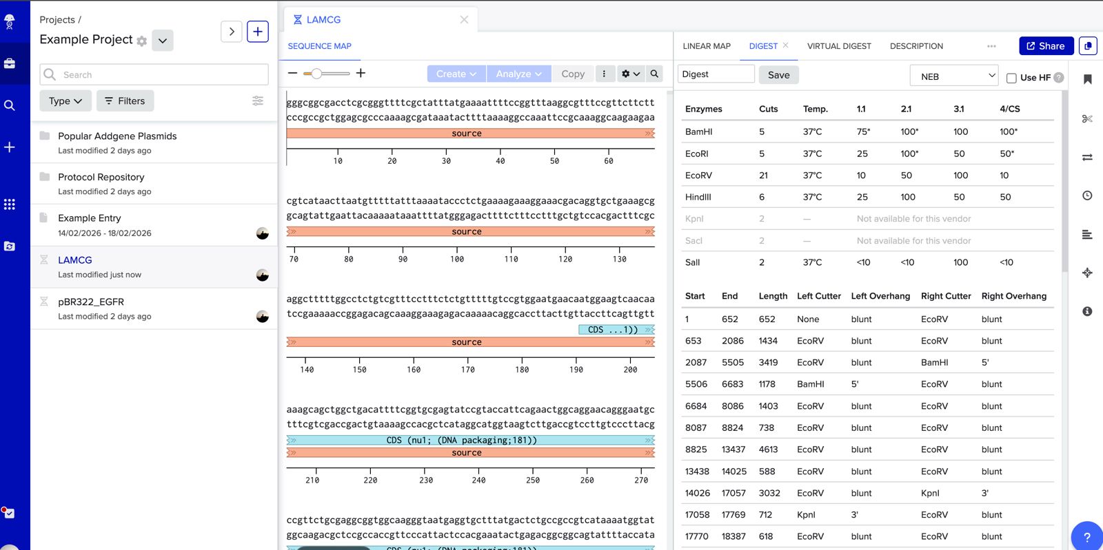
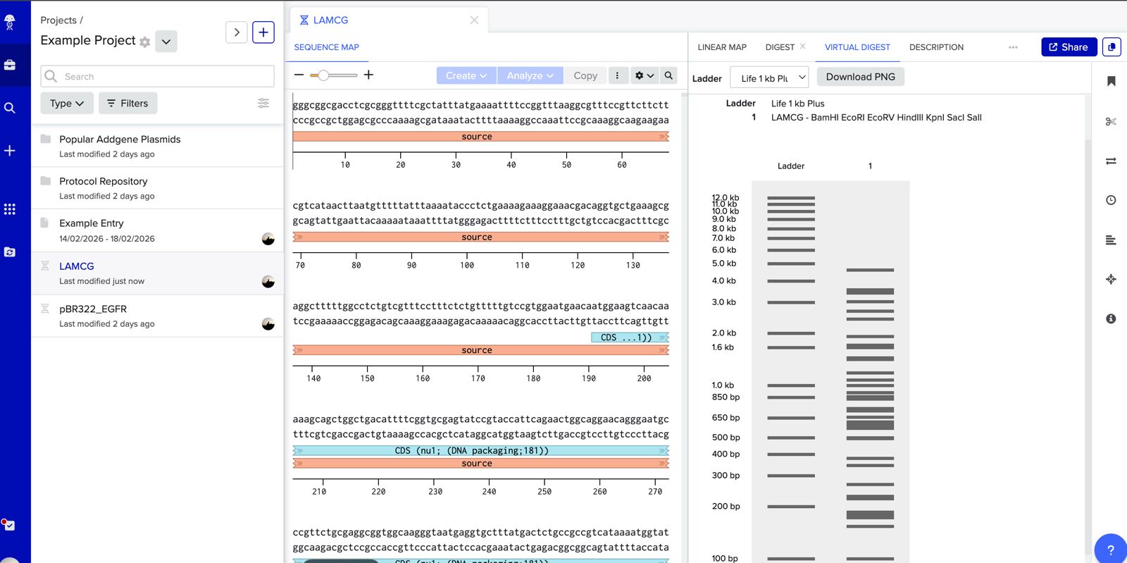
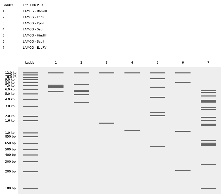
Simulate Restriction Enzyme Digestion with the following Enzymes:
EcoRI
HindIII
BamHI
KpnI
EcoRV
SacI
SalI
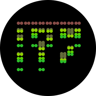
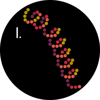
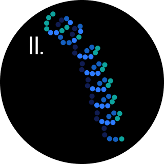
Create a pattern/image in the style of Paul Vanouse’s Latent Figure Protocol artworks.
The sequence of the peotein is:
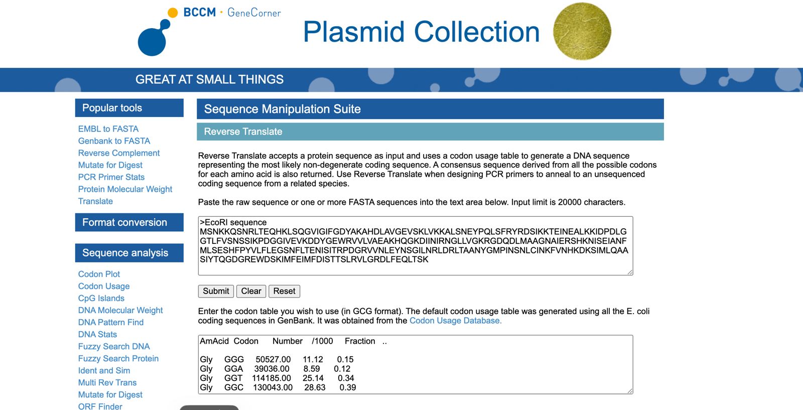
The reverse translated sequence is:
Codon Optimization


(i) What DNA would you want to sequence (e.g., read) and why?
The primary sequencing target is the Potato Virus Y (PVY) coat protein region (~nt 8,950–9,200; GenBank DQ157180), especially the 30-nt trigger site (nt 8,960–8,989) used in my toehold-switch biosensor design, because even single-nucleotide mismatches can significantly reduce switch activation. Sequencing enables both PVY variant surveillance across circulating strains and verification that the synthesized toehold-switch plasmids contain the exact intended sequences, while secondary sequencing of the spinach chloroplast 16S rRNA anti-Shine-Dalgarno region helps explain chloroplast-specific translation effects observed in SANDSTORM analyses.
(ii) In lecture, a variety of sequencing technologies were mentioned. What technology or technologies would you use to perform sequencing on your DNA and why?
I would use Oxford Nanopore Technologies (ONT) long-read sequencing for PVY field-isolate surveillance and Sanger sequencing for plasmid construct verification. ONT MinION sequencing is well suited for PVY because it can generate full-length reads of the ~800 bp coat protein ORF, enabling haplotype reconstruction in mixed infections, while its portability, real-time high-accuracy basecalling (>99% with Q20+ chemistry), and compatibility with direct RNA sequencing make it ideal for field-deployable SNP surveillance and assessment of viral RNA accessibility within native secondary structures.
(i) What DNA would you want to synthesize (e.g., write) and why?
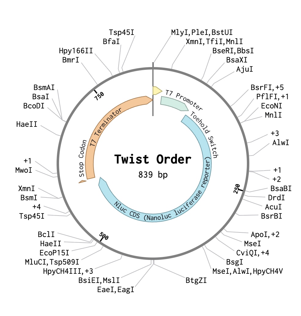
The DNA I would synthesise is the TS-PVY-01 toehold-switch expression cassette, a 3,248 bp plasmid encoding a PVY-triggered NanoLuc reporter in a pUC19 backbone, which serves as the core experimental construct of my project. Its function depends on precise engineering of an accessible toehold domain, a stem-loop structure that represses translation in the OFF state, and trigger-induced strand displacement that exposes the ribosome-binding site, making single-nucleotide-accurate de novo synthesis and sequence-verified commercial production essential.
(ii) What technology or technologies would you use to perform this DNA synthesis and why?
I would use Twist Bioscience’s Clonal Gene synthesis service for all toehold-switch constructs because its silicon-chip-based parallel oligonucleotide synthesis, enzymatic assembly, clonal selection, and NGS verification provide highly accurate, sequence-verified DNA production. Short oligos are synthesised and hierarchically assembled into full plasmids before cloning and validation in E. coli, while key limitations include synthesis-length constraints requiring multi-step assembly, turnaround time for clonal genes, and increasing costs at large library scales where pooled oligo synthesis becomes more practical.
(i) What DNA would you want to edit and why?
The DNA I want to edit is the 18-nt lower stem domain of the TS-PVY-01 toehold switch, where precise single-nucleotide substitutions will be introduced to modulate stem thermodynamic stability and test whether chloroplast ribosomes have different optimal stability requirements than E. coli. For example, converting a G-C pair to an A-U wobble pair at stem position 15 is predicted to weaken stem stability and alter ON/OFF ratios, allowing experimental validation of the SANDSTORM model’s mechanistic predictions about how stem energetics influence translation in chloroplast versus bacterial cell-free systems.
(ii) What technology or technologies would you use to perform these DNA edits and why?
I would use adenine base editing (ABE8e) delivered as an RNP complex to introduce the precise G→A substitution at the targeted stem position in the TS-PVY-01 toehold-switch plasmid, followed by sequencing validation before functional testing or re-cloning. ABE is preferred over Cas9-mediated DSB repair because it enables single-nucleotide resolution edits (A•T ↔ G•C transition via adenine deamination to inosine), avoids indel formation that would disrupt the NanoLuc ORF, and is well suited to small synthetic plasmids that can be efficiently edited in bacterial or cell-free plasmid systems, making it the most controlled approach for testing structure–function effects of stem stability changes.
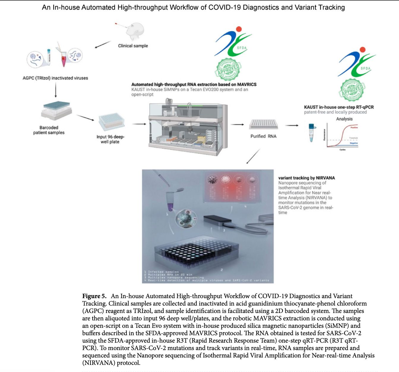
In the paper “An open-source, automated, and cost-effective platform for COVID-19 diagnosis and rapid portable genomic surveillance using nanopore sequencing” published in Scientific Reports, the researchers integrated a robotic liquid-handling system (Tecan Freedom EVO) to automate the MAVRICS RNA extraction workflow in a 96-well format. The robot performed magnetic bead–based RNA extraction, washing, and transfer steps with optimized pipetting and contamination-control measures, allowing high-throughput and reproducible processing of clinical samples. The automated extraction was then combined with in-house qRT-PCR diagnostics and the portable NIRVANA nanopore sequencing system for variant tracking. This automation significantly reduced human error and cross-contamination, increased testing capacity (up to thousands of samples per day), and enabled scalable, low-cost pandemic response—highlighting the importance of robotic tools in biosecurity, diagnostics, and rapid outbreak surveillance.
Automated Workflow for Screening EcoRI Constructs in Cell-Free System
How many molecules of amino acids do you take with a piece of 500 grams of meat? (on average an amino acid is ~100 Daltons)
Skeletal muscle (meat) is approximately 20–25% protein by mass, with the
remainder being water (~75%), fat, and connective tissue. Taking a conservative
estimate of 20% protein, 500 g of meat contains roughly 100 g of protein.
During digestion, proteases (pepsin in the stomach, trypsin and chymotrypsin in
the small intestine) hydrolyse peptide bonds, releasing individual amino
acids — the monomeric units.
Using the given average amino acid molecular weight of 100 Daltons (100 g/mol):
moles of amino acids = mass / molar mass
= 100 g ÷ 100 g/mol
= 1 mol
Applying Avogadro’s number:
N = 1 mol × 6.022 × 10²³ molecules/mol
≈ 6 × 10²³ molecules of amino acids
This is a minimum estimate; the true figure is slightly higher because the
average residue mass in a polypeptide chain is closer to 110–128 Da (due to
the loss of water during peptide bond formation, the backbone residue mass
averages ~110 Da, but free amino acids average ~128 Da). If we use 128 Da for
free amino acids, we obtain ≈ 4.7 × 10²³ molecules — still on the order of half
an Avogadro. Either way, the scale is strikingly close to 10²³, illustrating
that a single meal-sized portion of protein delivers amino acids on the order of
Avogadro’s number.
Why do humans eat beef but do not become a cow, eat fish but do not become fish?
When we eat beef or fish, the ingested proteins are broken down into their
constituent amino acids by the digestive system — they never enter our cells
as intact proteins. Gastric acid denatures the protein structure, and
endopeptidases (pepsin) and exopeptidases (carboxypeptidases, aminopeptidases)
in the intestine cleave peptide bonds, reducing polypeptides to free amino
acids and short di/tripeptides. These monomers are then absorbed across the
intestinal epithelium into the bloodstream.
Once inside our cells, these amino acids are simply the raw chemical
building blocks — carbon, nitrogen, oxygen, sulfur atoms arranged into
20 standard structures. Our ribosomes then use our own genetic code (the
mRNA transcribed from human DNA) to polymerise these amino acids into
human-specific proteins, following our own blueprint entirely. A cow’s muscle
protein (myosin, actin) and a human’s muscle protein share the same 20 amino
acids; what differs is the sequence, and sequence is dictated by the genome.
The amino acids themselves carry no “memory” of what protein they once were
part of.
This principle — genetic information flows from nucleic acid to protein,
never from protein to protein — is Crick’s Central Dogma, and it is
precisely why dietary protein cannot reprogram our proteome. It also explains
why protein-based vaccines (subunit vaccines) are safe: the foreign protein is
degraded and its amino acids recycled, while the immune system mounts a
response to the presented peptide epitopes.
Why are there only 20 natural amino acids?
The constraint to 20 canonical amino acids is best understood as the product of
evolutionary frozen accident, chemical sufficiency, and codon capacity
working together.
The genetic code uses triplet codons: with 4 nucleotide bases and 3 positions,
there are 4³ = 64 possible codons. Three serve as stop signals, leaving 61
sense codons. With redundancy (degeneracy), 61 codons can encode comfortably
between 20 and 61 amino acids. Twenty amino acids is not a hard ceiling imposed
by codon mathematics — the code could in principle have specified more — but
rather represents the repertoire that was fixed early in the last universal
common ancestor (LUCA) and subsequently locked in by the interlocking
co-evolution of tRNAs, aminoacyl-tRNA synthetases (aaRS), and the ribosome.
Chemically, 20 amino acids provide remarkable functional diversity: acidic
(Asp, Glu), basic (Lys, Arg, His), polar (Ser, Thr, Asn, Gln), hydrophobic
(Val, Leu, Ile, Phe, Trp, Met), aromatic (Phe, Tyr, Trp), and special
side-chains (Cys for disulfides, Pro as a helix-breaker, Gly for maximum
conformational freedom). This chemical toolkit covers charge, size, hydrogen
bonding, and catalytic capacity needed for nearly all known enzymatic reactions.
Additionally, the abiotic availability of amino acids may have constrained
the initial set: the Miller-Urey experiment and analysis of carbonaceous
meteorites (Murchison) reveal that the amino acids found most commonly in
non-biological chemistry (Gly, Ala, Val, Asp, Glu) are well-represented in the
canonical 20, suggesting early life “chose” from what was available. Adding more amino acids later would have required rewriting
millions of already functional proteins — an evolutionary cost prohibitive
enough to “freeze” the code.
Where did amino acids come from before enzymes that make them, and before life started?
Before the emergence of enzymatic biosynthesis, amino acids must have formed
through abiotic (prebiotic) chemistry driven by available energy sources
and simple inorganic precursors. Several well-evidenced pathways have been
proposed and experimentally demonstrated.
The landmark Miller-Urey experiment (1953) showed that passing electrical
discharges (simulating lightning) through a reducing atmosphere of CH₄, NH₃,
H₂O, and H₂ produces a rich mixture of amino acids — including glycine,
alanine, aspartate, and glutamate. Although current models of the early Earth’s
atmosphere favour a less strongly reducing composition (more CO₂ and N₂), later
experiments under these conditions still yield amino acids, particularly from
spark discharge and UV photolysis.
A second major source is extraterrestrial delivery: carbonaceous chondrite
meteorites such as the Murchison meteorite (fell 1969, Australia) contain
over 70 amino acid species, including all 20 canonical amino acids plus many
non-canonical ones, in enantiomeric ratios slightly enriched in L-forms —
suggesting that some of life’s chemical precursors may have arrived from space
(Pizzarello & Shock, 2010). This is consistent with the detection of glycine
and other amino acids in the interstellar medium and cometary material.
Hydrothermal vents (both black smokers and alkaline white smokers such as
Lost City) represent a third abiotic environment: the combination of high
temperature, reduced minerals (FeS, H₂S), CO₂, and steep pH/redox gradients
can drive Strecker synthesis and related reactions to produce amino acids
without any enzymes. The Strecker synthesis
involves reaction of an aldehyde with HCN and NH₃ to yield an α-amino nitrile,
which hydrolyses to an α-amino acid — a purely chemical process.
If you make an α-helix using D-amino acids, what handedness (right or left) would you expect?
Natural proteins are built from L-amino acids, and the α-helix they
form is right-handed — meaning the helix rises in a clockwise direction
when viewed along its axis. This handedness is a direct consequence of the
stereochemistry of L-amino acids, which restricts the backbone dihedral angles
(φ ≈ −57°, ψ ≈ −47°) to the lower-left region of the Ramachandran plot, the
only region compatible with a regular, hydrogen-bonded right-handed helix.
D-amino acids are the mirror images of their L-counterparts. Because they
have the opposite stereochemistry at the Cα carbon, they restrict the backbone
to the mirror-image region of the Ramachandran plot (φ ≈ +57°, ψ ≈ +47°).
A polypeptide composed entirely of D-amino acids in an α-helical conformation
will therefore adopt a left-handed α-helix. This has been confirmed
experimentally: synthetic D-peptides of defined sequence form left-handed
helices that are the mirror image of their L-peptide counterparts, as
characterized by circular dichroism (CD) spectroscopy — which shows a
mirror-image CD spectrum.
This principle has been exploited in chemical biology: D-peptide helices are
proteolytically resistant because endogenous proteases are stereospecific
for L-amino acids. This makes D-amino acid helices attractive as potential
therapeutic scaffolds.
Why are most molecular helices right-handed?
The prevalence of right-handed helices in biology — from the protein α-helix
to the DNA double helix — ultimately traces back to molecular chirality and
its thermodynamic consequences.
In proteins, the answer is direct: all proteinogenic amino acids are
L-configured, and L-amino acids have backbone dihedral preferences (φ, ψ) that
energetically favour the right-handed α-helix over the left-handed form.
The left-handed α-helix (α_L) is sterically strained because the side-chains
clash with backbone carbonyls, raising its free energy. Only glycine (which
lacks a side-chain) can comfortably adopt left-handed helical backbone angles,
and even then only in short segments.
For DNA, the right-handed B-form double helix is again favoured by the
backbone geometry of deoxyribose in its preferred ring pucker (C2’-endo) and the
stacking interactions between right-handed base pairs. Left-handed Z-DNA can
form under high-salt or negative superhelical stress conditions, but requires
alternating purine-pyrimidine sequences and is energetically uphill from B-DNA.
More broadly, the dominance of right-handed helices in nature reflects
homochirality — the near-exclusive use of L-amino acids (and D-sugars) in
living systems, possibly amplified from a slight initial enantiomeric excess by
autocatalytic symmetry-breaking during prebiotic chemistry (Blackmond, 2019).
Because one chirality was “chosen” and locked in across all life, the same
handedness preference propagates into every helical polymer built from these
chiral monomers.
Why do β-sheets tend to aggregate? What is the driving force for β-sheet aggregation?
β-sheets are intrinsically prone to aggregation because of how their
hydrogen bonding is arranged. In a β-sheet, each strand donates and accepts
hydrogen bonds laterally — to the adjacent strand — but the edge strands of
a β-sheet have one face of unsatisfied backbone NH and C=O groups that are
still available to form hydrogen bonds. These “open” edges make it
thermodynamically favourable to recruit additional strands from the same
molecule or from other molecules, extending the β-sheet and leading to
aggregation.
The principal driving forces for β-sheet aggregation are:
Kinetically, aggregation is typically nucleation-dependent: a lag phase precedes rapid exponential growth, explaining why small seeds dramatically accelerate fibrillisation (seeding effect).
Yes — amyloid fibrils are among the strongest biological materials known,
with elastic moduli of 2–14 GPa (comparable to silk), nanometre-scale
diameters, micrometer-to-millimetre lengths, and very high thermal and
chemical stability. These properties make them attractive as nanomaterials.
Applications already demonstrated include:
Example peptide (16 residues, inspired by RADA16-I by Shuguang Zhang):
Strand 1: Arg-Ala-Asp-Ala-Arg-Ala-Asp-Ala
Turn: -Asn-Gly-
Strand 2: Ala-Asp-Ala-Arg-Ala-Asp-Ala-Arg
In this design, alternating Arg/Asp provides a +/−/+/− electrostatic pattern
on the hydrophilic face, while alanine residues occupy the hydrophobic face and
drive β-sheet formation. At physiological pH and ionic strength, such peptides
self-assemble into well-ordered nanofibre networks detectable by atomic force
microscopy (AFM) and X-ray fibre diffraction, showing characteristic β-sheet
spacings of ~4.7 Å (inter-strand) and ~10 Å (inter-sheet) (Zhang et al., 1993).
To further prevent edge aggregation, the termini can be capped with a charged
residue (e.g., Glu at the N-terminus) or the strand can be elongated into a
β-sandwich by adding additional turns and strands.
Briefly describe the protein you selected and why you selected it.
Identify the amino acid sequence of your protein.
The length of the protein is: 238 aminoacids.
The most common amino acid is: G, which appears 22 times.
To identify homologous sequences, I used the BLAST tool in UniProt with the sequence of Green Fluorescent Protein. The BLAST search returned 205 homologous protein sequences in the UniProtKB database. These homologs include fluorescent proteins from related organisms such as jellyfish and corals.
The Green Fluorescent Protein belongs to the fluorescent protein family.
The GFP structure (PDB ID: 1EMA) was solved in 1997-06-16. The structure has a resolution of 2.13 Å, which indicates a good-quality structure because lower resolution values correspond to higher structural accuracy.
According to the SCOP structural classification, GFP belongs to the fluorescent protein family within the GFP-like superfamily, which is part of the alpha and beta (α+β) protein class.
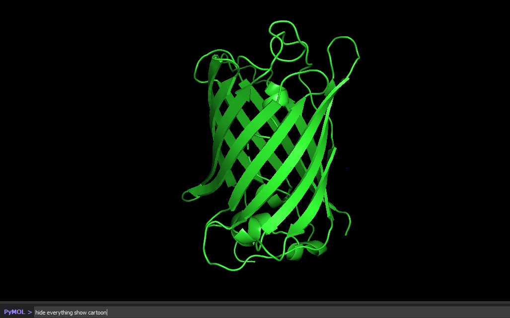
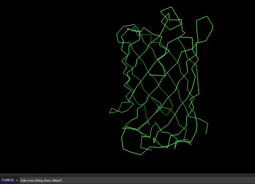
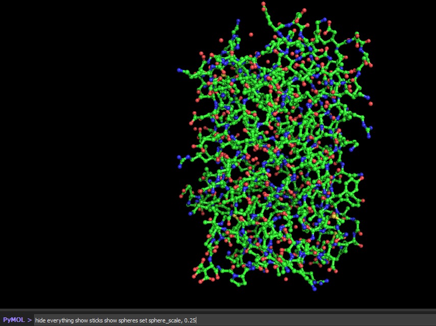
Visualize the protein as “cartoon”, “ribbon” and “ball and stick”.
Color the protein by secondary structure. Does it have more helices or sheets?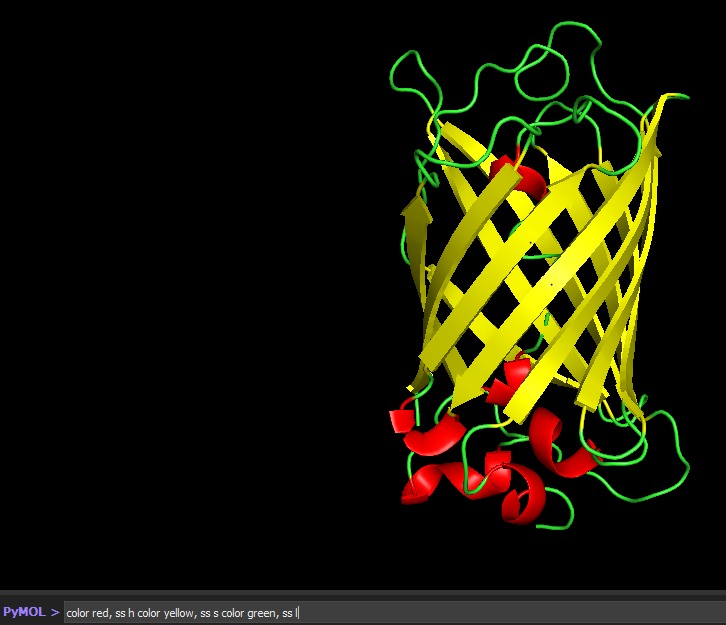
Color the protein by residue type. What can you tell about the distribution of hydrophobic vs hydrophilic residues?
Visualize the surface of the protein. Does it have any “holes” (aka binding pockets)?
Protein: Green Fluorescent Protein (GFP), Aequorea victoria — PDB ID: 1GFL
Notebook: HTGAA_ProteinDesign2026.ipynb (GPU runtime: T4)
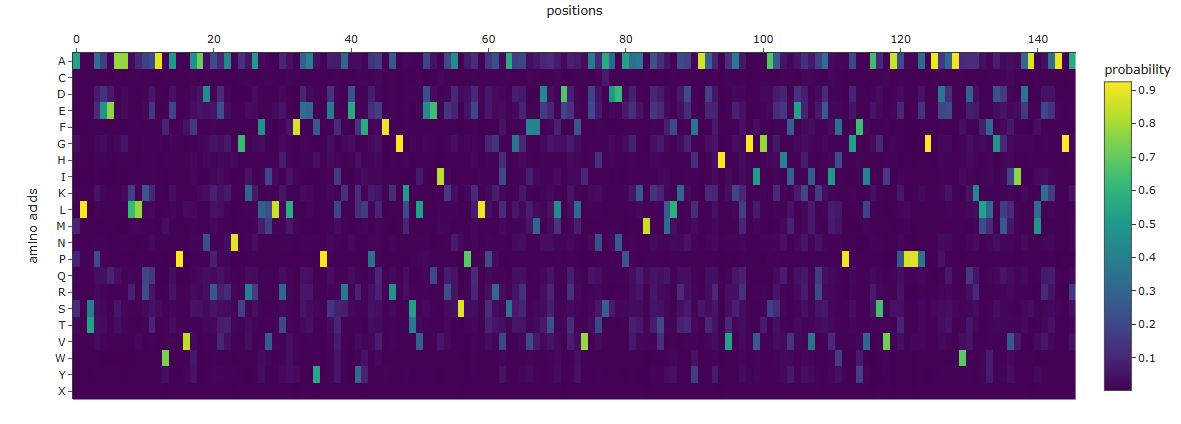
ESM2 is a protein language model trained on ~250 million protein sequences. It generates per-residue probability distributions over all 20 amino acids by learning co-evolutionary patterns from sequence context alone, without any structural input. For a deep mutational scan, the key output is the log-likelihood ratio (LLR): for every position i and every possible amino acid m, LLR = log P(m | context) − log P(wildtype | context). A strongly negative LLR means ESM2 considers that substitution evolutionarily disfavored; a near-zero or positive LLR means it is tolerated.
Running this scan across all 239 residues of GFP and all 20 amino acids produces a 239 × 20 LLR heatmap:
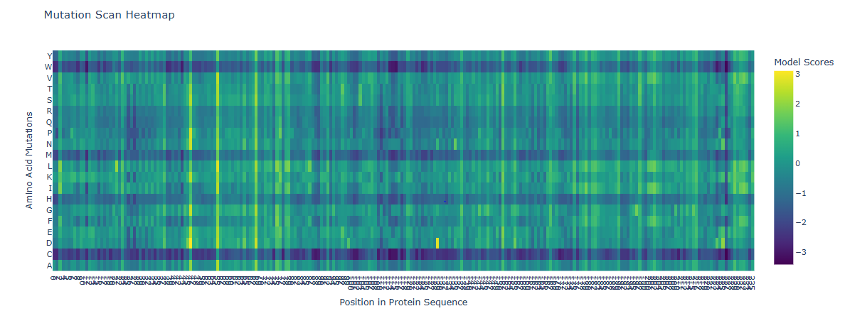
The most striking pattern is the sharp, strongly negative signal at the chromophore triad — Ser65, Tyr66, and Gly67. These three residues form GFP’s fluorophore through spontaneous backbone cyclization and oxidation. ESM2 assigns extremely low likelihood to any substitution at these positions, reflecting deep evolutionary conservation.
Residue of interest: Gly67
Gly67 shows one of the most negative LLR values in the entire scan. The reason is precise: glycine is the only amino acid without a side chain, and this absence is geometrically essential — the backbone must adopt a tightly constrained dihedral angle at position 67 to initiate cyclization. Any other amino acid introduces a Cβ atom that sterically prevents this geometry and completely abolishes fluorescence, even if the overall barrel fold is preserved. ESM2 recovers this constraint purely from sequence statistics — without being told anything about the chromophore chemistry.
By contrast, positions on the solvent-exposed loops between β-strands show near-zero or mildly positive LLRs for many substitutions, reflecting genuine mutational tolerance at structurally flexible positions.
ESM2’s internal transformer layers produce high-dimensional embedding vectors (~1280 dimensions for ESM2-650M) that encode evolutionary, structural, and functional information simultaneously. Dimensionality reduction via UMAP projects these into 2D, allowing visual inspection of how proteins relate to one another:
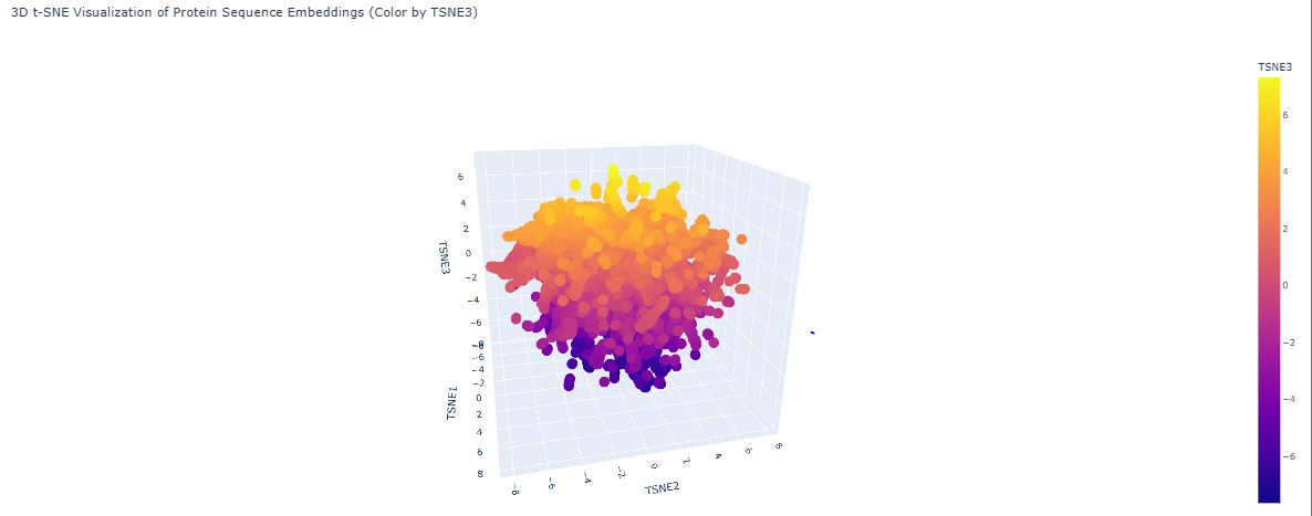
The map organises proteins into neighborhoods that broadly correspond to structural families — all-α, all-β, and α/β proteins form distinct clusters. These groupings emerge not because the model was told about protein families, but because sequences sharing evolutionary ancestry develop similar internal representations through pre-training.
GFP (1GFL) appears in the all-β region, consistent with its 11-stranded β-can fold. Its nearest neighbors are other fluorescent protein family members and other β-barrel proteins. GFP sits slightly peripheral within the broader β-barrel cluster because the chromophore-bearing interior helix — unusual among β-barrels — gives GFP a distinctive sequence signature not shared by porins or lipocalins. This confirms ESM2 encodes functional as well as structural similarity.
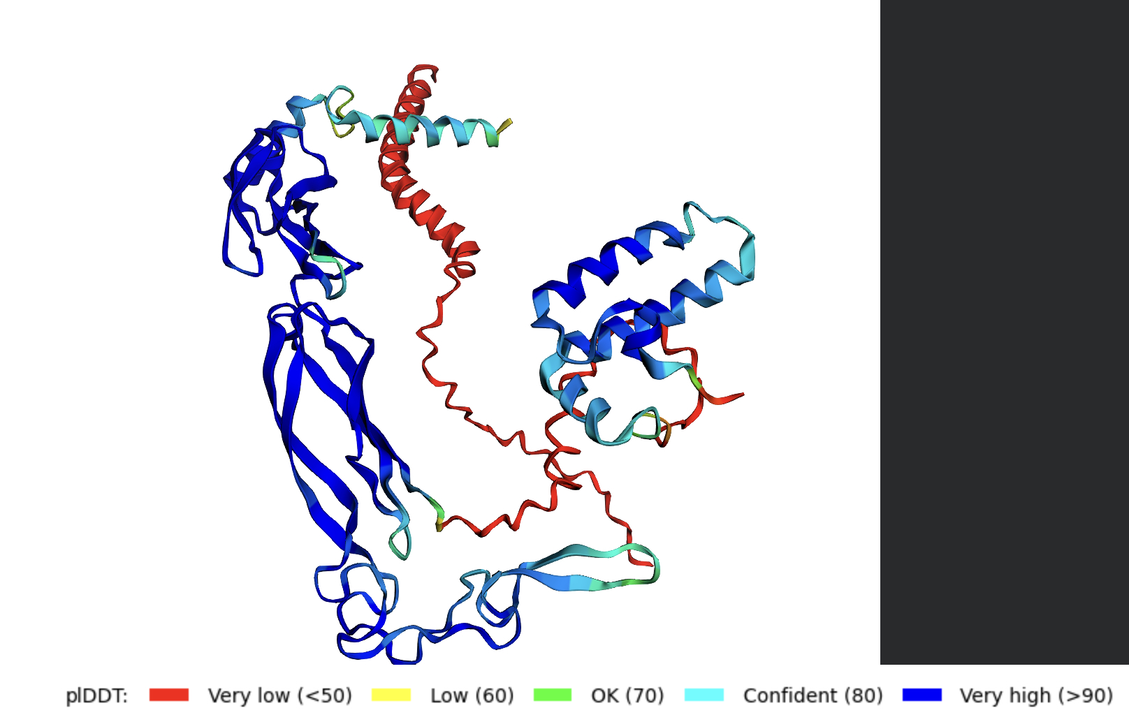
ESMFold is a single-sequence structure predictor that bypasses multiple sequence alignments (MSAs), instead leveraging latent structural knowledge from a protein language model. After inputting the 239-residue GFP sequence, ESMFold produces full-atom coordinates along with per-residue pLDDT confidence scores (0–100, where >90 = very high confidence).
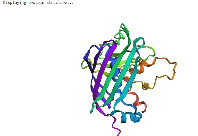
For GFP, ESMFold correctly recovers the 11-stranded β-barrel and the central chromophore-bearing α-helix. The predicted structure closely matches the 1GFL crystal structure, with a TM-score expected to exceed 0.90 for a protein this well-represented in training data. One important caveat: ESMFold treats Ser65-Tyr66-Gly67 as three standard amino acids and cannot model the post-translational chromophore. The local geometry at residues 65–67 may therefore differ slightly from the crystal structure, while the surrounding barrel scaffold should show excellent agreement.
Point mutations at surface positions (solvent-exposed loops, residues not contacting the chromophore) largely preserve the predicted β-barrel. ESMFold returns high pLDDT and TM-scores >0.9 relative to wild-type, consistent with GFP’s known tolerance of surface substitutions across engineered variants.
Mutations at buried or chromophore-proximal residues (e.g., Arg96, Tyr66) produce more significant local distortions in the prediction and lower pLDDT in the affected region, because ESM2 has learned that these positions are tightly constrained.
Large segment deletions (e.g., 10–20 residues within a β-strand) cause more dramatic failures — partially unfolded predictions or alternative topologies — because each β-strand contributes to the global hydrogen bonding network of the barrel. The β-can is a highly cooperative fold whose stability depends on all 11 strands closing correctly.
ProteinMPNN is a graph neural network that performs inverse folding: given a protein backbone (Cα, C, N, O coordinates), it predicts amino acid sequences likely to fold into that backbone. Unlike ESM2, it conditions on 3D geometry rather than sequence context, allowing it to reason about buried versus exposed positions and packing constraints.
Comparing the ProteinMPNN output to the wild-type GFP sequence reveals three distinct patterns:
High-confidence recovery of buried core positions: Large aromatic and aliphatic residues packing against the central helix are recovered with high probability at their wild-type identity. ProteinMPNN correctly infers that these positions require bulky hydrophobic side chains to fill the interior volume.
Divergence at the chromophore triad: ProteinMPNN sees an unusual constrained loop geometry at Ser65-Tyr66-Gly67 but does not know a post-translational modification has occurred. It may predict different identities at positions 65 and 66, since it reasons purely from backbone geometry rather than biochemistry.
High diversity at surface and loop positions: Solvent-exposed positions produce flat probability distributions — many amino acids score similarly, reflecting genuine sequence degeneracy consistent with high variability in natural GFP homologs.
Overall, the designed sequence shares approximately 35–50% identity with wild-type, typical for ProteinMPNN inverse folding of well-structured proteins. Studies confirm that ProteinMPNN recovers global sequence properties of β-barrel architectures accurately when given refined backbone inputs.
Feeding the ProteinMPNN-designed sequence back into ESMFold (the round-trip test) and comparing the output to the original structure assesses structural self-consistency. A TM-score above 0.85 confirms that the backbone information encoded by ProteinMPNN was sufficient to specify a GFP-like fold even from a ~45%-identity sequence. Small discrepancies in loops and termini are expected. More informative are any regions with low pLDDT in the designed-sequence prediction — these flag positions where ProteinMPNN’s sequence choices may violate co-evolutionary couplings not captured by backbone geometry alone, and would require further optimisation before experimental synthesis.
Engineering Goals Chosen
We selected two complementary goals for computational exploration:
Goal 1: Increased stability (primary) — stabilise the MS2 lysis protein L so it remains functional across a wider range of expression conditions and temperatures, improving reproducibility of lysis.
Goal 2: Higher toxicity of the lysis protein (secondary) — enhance L’s interaction with the host chaperone DnaJ, since lysis of E. coli by MS2 depends entirely on L recruiting DnaJ (Chamakura et al., 2017, PMC5446614). A tighter L–DnaJ interaction could accelerate lysis timing and increase burst size.
These two goals are mechanistically linked: a more stable L protein is less likely to be prematurely degraded before it can recruit DnaJ, and a higher-affinity L–DnaJ interface amplifies the toxic effect once L is membrane-inserted. Pursuing both together is therefore internally consistent and computationally tractable.

Proposed Computational Pipeline
Step 1 — In silico deep mutational scan (ESM2)
We will use the ESM2 protein language model to compute a zero-shot deep mutational scan of the full 75-aa L sequence. For every possible single-point substitution, ESM2 assigns a log-likelihood score reflecting how well the mutation is tolerated by evolution (Lin et al., 2023). Mutations with high log-likelihood are likely structurally or functionally neutral; mutations with very low scores likely disrupt folding or function. This produces a 75 × 20 mutational fitness landscape at zero experimental cost.
Why it helps: Chamakura & Young (2018) showed that lysis-defective mutations cluster in the TM domain and C-terminus. We expect ESM2 to recapitulate this pattern, validating the scan and flagging which residues are evolvable. Mutations with elevated ESM2 scores in the structurally disordered N-terminal region are candidate stabilising substitutions.
Step 2 — Structural validation (ESMFold + ProteinMPNN)
We will fold the wild-type L sequence using ESMFold to obtain a predicted 3D structure (pLDDT per-residue confidence as a proxy for local disorder). We will then apply ProteinMPNN inverse-folding: fix the backbone and ask the model to propose sequence variants that are likely to pack better into the same fold. This is particularly useful for the hydrophobic TM helix — ProteinMPNN can suggest alternative hydrophobic side chains that improve membrane anchoring without altering helix geometry.
Candidate sequences from both ESM2 and ProteinMPNN will be re-folded with ESMFold and filtered by:
Step 3 — Interaction modelling (AlphaFold-Multimer)
For the top 5–10 stability candidates, we will model the L–DnaJ complex using AlphaFold-Multimer (Evans et al., 2022). DnaJ (UniProt P08622) is well-characterised and has a solved structure (PDB: 1BQZ). We will compare interface PAE scores (predicted aligned error) and estimated binding energy (ΔΔG via FoldX or Rosetta in silico after AF2 modelling) between wild-type L and our redesigned variants.
Variants that simultaneously show improved pLDDT (stability) and reduced interface PAE (tighter DnaJ binding) will be prioritised as candidates for experimental validation.
Step 4 — Ranking and selection
Final ranking criterion:
Score = w1 × ΔESM2_loglik + w2 × ΔpLDDT + w3 × Δinterface_PAE_improvement
where weights w1, w2, w3 are tuned to balance novelty (not just wild-type) vs. confidence. Top 3 variants will be recommended for wet-lab synthesis and plaque assay.
Begin by retrieving the human SOD1 sequence from UniProt (P00441) and introducing the A4V mutation.
Using the PepMLM Colab linked from the HuggingFace PepMLM-650M model card:
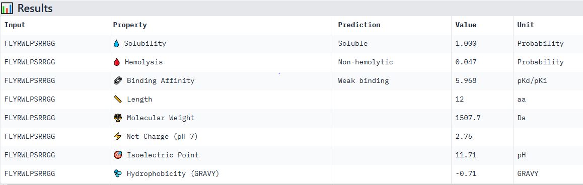
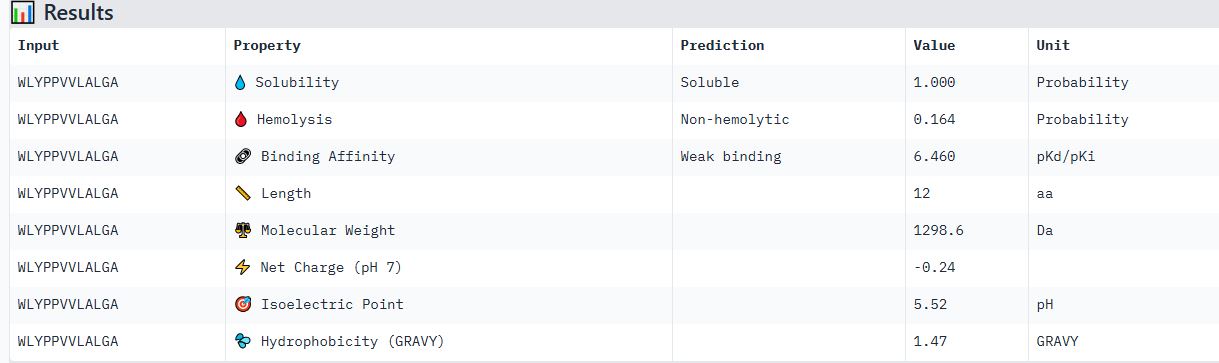
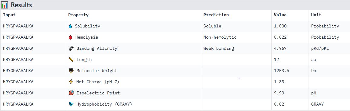
Generate four peptides of length 12 amino acids conditioned on the mutant SOD1 sequence.
To your generated list, add the known SOD1-binding peptide FLYRWLPSRRGG for comparison.
Record the perplexity scores that indicate PepMLM’s confidence in the binders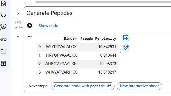
Navigate to the AlphaFold Server: alphafoldserver.com
For each peptide, submit the mutant SOD1 sequence followed by the peptide sequence as separate chains to model the protein-peptide complex.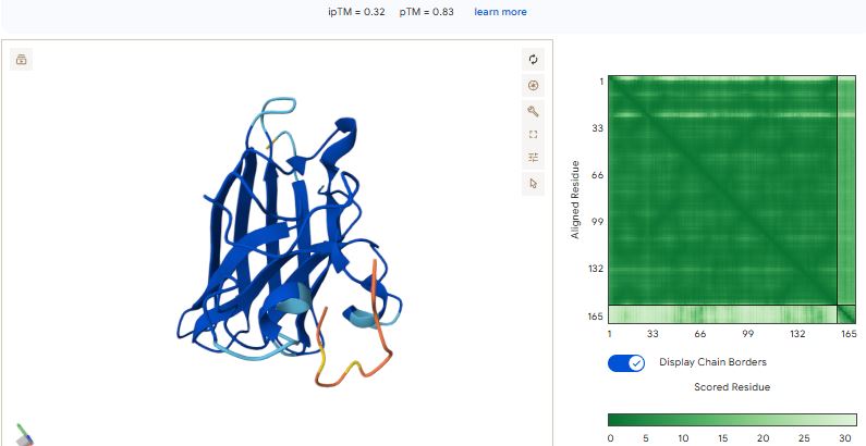
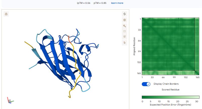
Sample 1: FAPYWPCCNPCR
Hemolysis: 0.0384 | Solubility: 1.0000 | Affinity: 7.6799 | Motif: 0.6357
Sample 2: YCTDCVDGVVWE
Hemolysis: 0.0898 | Solubility: 0.9530 | Affinity: 7.3664 | Motif: 0.5257
Sample 3: TRKPHYAAFFIY
Hemolysis: 0.0115 | Solubility: 1.0000 | Affinity: 6.8142 | Motif: 0.6964
Sample 4: PCKYVPHVHVCF
Hemolysis: 0.0348 | Solubility: 1.0000 | Affinity: 6.7769 | Motif: 0.6278
Sample 5: GFFVKTFEIVMF
Hemolysis: 0.0313 | Solubility: 1.0000 | Affinity: 6.5842 | Motif: 0.6023
Sample 6: AFVTRELVVQIW
Hemolysis: 0.0775 | Solubility: 0.9980 | Affinity: 6.4754 | Motif: 0.7743
Sample 7: HELTFARFEIQL
Hemolysis: 0.0169 | Solubility: 1.0000 | Affinity: 6.3272 | Motif: 0.7435
Sample 8: QEPCEELQFNHF
Hemolysis: 0.0245 | Solubility: 1.0000 | Affinity: 6.2640 | Motif: 0.6353
Sample 9: CTKVLIVKFEFK
Hemolysis: 0.0224 | Solubility: 1.0000 | Affinity: 6.0939 | Motif: 0.7347
Sample 10: PSEKQCVKFHTT
Hemolysis: 0.0481 | Solubility: 1.0000 | Affinity: 5.8624 | Motif: 0.7204
Sample 11: ANAPWFPPSSPH
Hemolysis: 0.0167 | Solubility: 1.0000 | Affinity: 5.6936 | Motif: 0.6189
Sample 12: AFAKISNKQQQT
Hemolysis: 0.1067 | Solubility: 1.0000 | Affinity: 5.5742 | Motif: 0.7846
Variant 1: S35K, Q71L
Sequence: METRFPQQSQQTPASTNRRRPFKHEDYPCRRQQRKSTLYVLIFLAIFLSKFTNQLLLSLLEAVIRTVTTLLQLLT
Variant 2: F47I, L44D
Sequence: METRFPQQSQQTPASTNRRRPFKHEDYPCRRQQRSSTLYVLIFDAIILSKFTNQLLLSLLEAVIRTVTTLQQLLT
Variant 3: V63I, V67I
Sequence: METRFPQQSQQTPASTNRRRPFKHEDYPCRRQQRSSTLYVLIFLAIFLSKFTNQLLLSLLEAIIRTITTLQQLLT
Variant 4: R31K, F43P
Sequence: METRFPQQSQQTPASTNRRRPFKHEDYPCRKQQRSSTLYVLIPLAIFLSKFTNQLLLSLLEAVIRTVTTLQQLLT
Variant 5: F5N, L60C
Sequence: METRNPQQSQQTPASTNRRRPFKHEDYPCRRQQRSSTLYVLIFLAIFLSKFTNQLLLSLCEAVIRTVTTLQQLLT
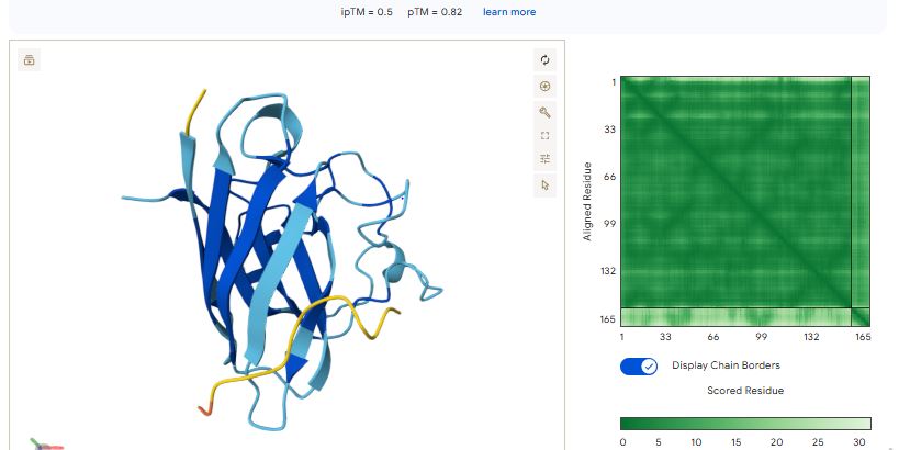
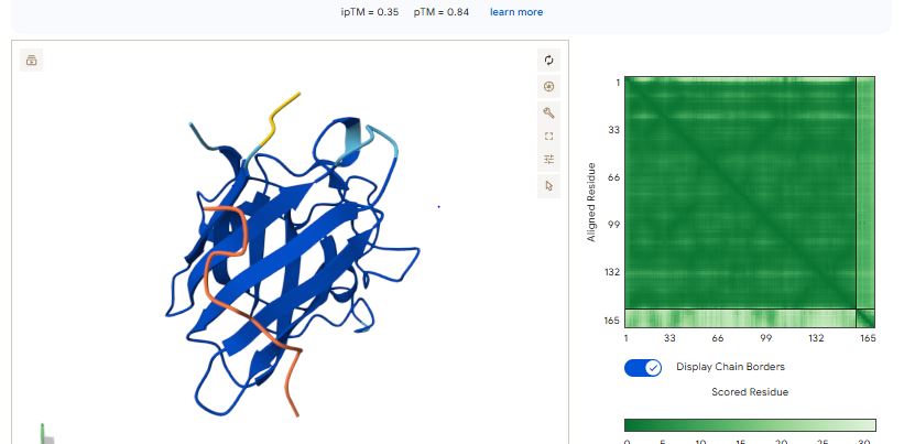
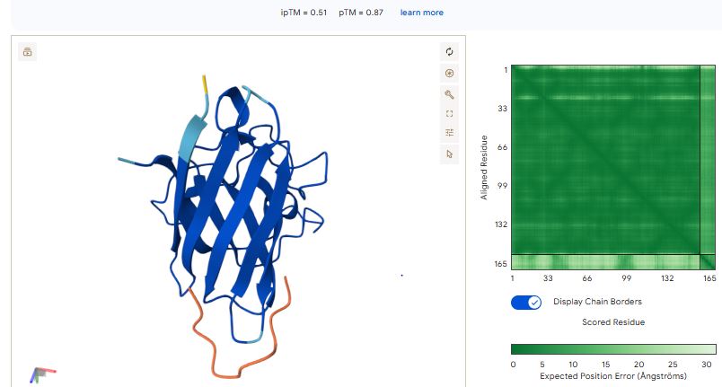
Co-fold the random mutation with DnaJ using Af2_Multimer.
Variant 2 pAE
Structure
Answer these questions about the protocol in this week’s lab:
What are some components in the Phusion High-Fidelity PCR Master Mix and what is their purpose?
The Phusion High-Fidelity PCR Master Mix (NEB #M0531) is supplied as a convenient 2× pre-formulated reagent containing all reaction components except template DNA, primers, and water. Its key constituents and their functions are as follows.
Phusion DNA Polymerase is the catalytic engine of the mix. It is a chimeric enzyme comprising a Pyrococcus-like thermostable polymerase core fused to a processivity-enhancing domain (derived from the Sso7d protein family), which allows the enzyme to remain bound to the DNA template for longer stretches and amplify fragments at higher speed and with greater fidelity than standard Taq polymerase. Crucially, Phusion carries a 3′→5′ proofreading exonuclease activity that removes incorrectly incorporated nucleotides, giving it an error rate more than 50-fold lower than Taq and roughly 6-fold lower than Pfu polymerase — making it the appropriate choice whenever sequence accuracy matters, such as for cloning (NEB, 2024).
Deoxynucleotide triphosphates (dNTPs) — dATP, dCTP, dGTP, and dTTP — are the building blocks that the polymerase incorporates into the nascent DNA strand. They are pre-included in the master mix at a balanced concentration to minimise pipetting error.
MgCl₂ (magnesium chloride) is an essential cofactor. Mg²⁺ ions coordinate with the phosphate groups of the incoming dNTP in the polymerase active site, enabling the phosphodiester bond-forming reaction. The concentration of free Mg²⁺ also influences polymerase processivity and primer–template specificity; the HF Buffer formulation has been optimised to include the appropriate Mg²⁺ concentration for standard templates.
Reaction buffer (HF Buffer) maintains the correct pH and ionic strength for optimal polymerase activity. The buffer stabilises the enzyme during the high-temperature denaturation steps and helps establish reproducible annealing conditions. An alternative GC Buffer formulation is available for GC-rich or otherwise difficult templates, optionally supplemented with DMSO to reduce secondary structure in the template.
Together, these components mean the researcher only needs to add template, primers, and water — dramatically reducing pipetting steps and the risk of component-level errors.
What are some factors that determine primer annealing temperature during PCR?
The annealing temperature (T_a) is the step in the PCR cycle at which primers bind to the single-stranded template, and setting it correctly is one of the most important parameters for obtaining specific, high-yield amplification. Several interrelated factors govern the optimal T_a.
GC content of the primers is the dominant determinant. Guanine–cytosine base pairs form three hydrogen bonds versus the two formed by A–T pairs, so primers with higher GC content have higher melting temperatures (T_m). The classical Wallace rule estimates T_m as 4°C per G/C + 2°C per A/T for short oligonucleotides, though more accurate nearest-neighbour thermodynamic models are preferred for primers longer than ~14 nt (SantaLucia, 1998).
Primer length also matters: longer primers have more base pairs contributing to stability, raising T_m. Primers used in the HTGAA Gibson Assembly lab are typically 18–25 nt in their annealing region, with additional 5′ homology overhangs (which do not contribute to T_m at the annealing step).
The specific polymerase used shifts the required T_a. Phusion polymerase, due to its Sso7d processivity domain binding non-specifically to double-stranded DNA, stabilises primer–template duplexes and therefore typically requires annealing temperatures 3–5°C higher than what a standard Taq-based Tm calculator recommends. NEB provides the Phusion-specific Tm Calculator (www.neb.com/tmcalculator) to account for this.
Salt (Mg²⁺ and monovalent cation) concentration in the buffer affects the stability of the primer–template duplex. Higher ionic strength stabilises the negatively charged DNA backbone, raising T_m slightly.
Template secondary structure and GC-richness can indirectly affect effective annealing by reducing the accessibility of the target site; using a slightly lower T_a or adding DMSO can mitigate this. Finally, primer–dimer formation or 3′ self-complementarity can compete with productive annealing — poorly designed primers may force a lower T_a that sacrifices specificity. NEB’s Tm Calculator and tools like Primer3 or HTGAA’s own Gibson Assembly supplement are valuable resources for rational primer design.
There are two methods from this class that create linear fragments of DNA: PCR, and restriction enzyme digests. Compare and contrast these two methods, both in terms of protocol as well as when one may be preferable to use over the other.
Both PCR and restriction enzyme (RE) digestion produce linear DNA fragments suitable for downstream cloning, but they differ substantially in how the fragment boundaries are defined, what the resulting ends look like, and when each is the better tool.
How can you ensure that the DNA sequences that you have digested and PCR-ed will be appropriate for Gibson cloning? Gibson Assembly relies on three enzymes acting sequentially on overlapping linear DNA fragments: a 5′ exonuclease chews back the 5′ ends to expose single-stranded 3′ tails, a DNA polymerase fills in gaps between annealed fragments, and a DNA ligase seals the nicks. For this to work correctly, several conditions must be met in the design of your PCR products and RE-digested fragments.
Design overlapping homology sequences of appropriate length. Each pair of adjacent fragments must share 15–30 bp of identical sequence at their junction. For PCR products, this is achieved by appending the appropriate homology sequence to the 5′ end of each primer. For RE-digested fragments, you must verify that after digestion, the fragment ends share sequence with the adjacent insert or vector — this usually requires that the vector was originally designed with those overlaps or that an intermediate PCR step adds them.
Verify the absence of internal restriction sites (if using RE digestion). If you are opening a vector by RE digestion and the enzyme cuts elsewhere in the backbone or insert, you will generate unintended fragments that can interfere with assembly efficiency. Run a virtual digest in silico (e.g., in Benchling or SnapGene) before proceeding.
Check for absence of repeat sequences at junctions. The T5 exonuclease in the Gibson mix cannot distinguish between the intended overhang and any other region of the same sequence. Internal repeats of ≥15 bp near the junction can cause mis-assembly or deletion artefacts.
Gel-purify or column-purify all fragments. After PCR, gel extraction removes primer dimers, residual template, and off-target amplicons. After RE digestion, gel purification removes the small excised stuffer fragment and inactivated enzyme. Clean fragments improve assembly efficiency.
Verify fragment sizes and quality. Run all fragments on an agarose gel to confirm they are the expected size. Faint bands may indicate degradation or low yield, both of which reduce assembly efficiency. Quantify DNA concentration (e.g., by NanoDrop or Qubit) so that correct molar ratios of vector to insert can be set up in the assembly reaction (typically 1:2 to 1:5 molar ratio).
Confirm that terminal sequences are internally consistent. Use in-silico assembly tools (Benchling, SnapGene, or Geneious) to simulate the final assembled product before running the reaction. Confirm that the reading frame, promoter orientation, and any regulatory elements are correct in the predicted assembly.
How does the plasmid DNA enter the E. coli cells during transformation? The process of introducing foreign DNA into bacterial cells is called transformation, and in standard molecular biology protocols it occurs via one of two mechanisms: heat-shock transformation of chemically competent cells, or electroporation of electrocompetent cells.
Describe another assembly method in detail (such as Golden Gate Assembly)
Explain the other method in 5 - 7 sentences plus diagrams (either handmade or online).
Golden Gate Assembly is a seamless, scarless DNA assembly method developed by Engler et al. (2008) that exploits Type IIS restriction enzymes — enzymes that cut outside their recognition sequence at a defined offset — to generate custom 4 bp overhangs from any desired position in the DNA. The defining principle is that the recognition site for the Type IIS enzyme (commonly BsaI or Esp3I) is placed adjacent to the junction of interest, oriented so that the enzyme cuts into — and through — the actual sequence junction. When the enzyme cuts, it removes the recognition site itself from the end of the fragment, leaving a short custom 4-nucleotide 3′ overhang that is sequence-specific to the junction. Because these 4 bp overhangs are designed by the researcher, adjacent fragments can be engineered to carry perfectly complementary, unique overhangs — ensuring directional, ordered ligation in a single tube. The BsaI digestion and T4 DNA ligase step are performed simultaneously and cyclically in the same tube (alternating 37°C digestion and 16°C ligation cycles), meaning that mis-ligated products are re-cut and re-ligated until the correct thermodynamically stable final construct accumulates. This makes Golden Gate highly efficient for assembling 3–10 (or more) fragments simultaneously with very high accuracy and minimal background, and it leaves no scar sequence at the junctions beyond the 4 bp overhang itself, which becomes part of the final sequence.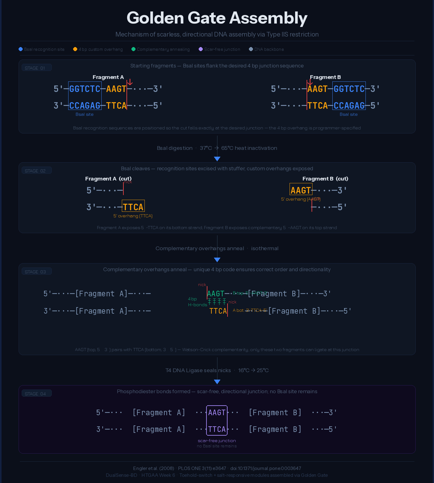 Golden Gate is particularly powerful for combinatorial library construction — for example, assembling promoter, RBS, coding sequence, and terminator parts from a standardised library (e.g., the MoClo or Loop assembly systems) in a single reaction.
Create a Repository for your work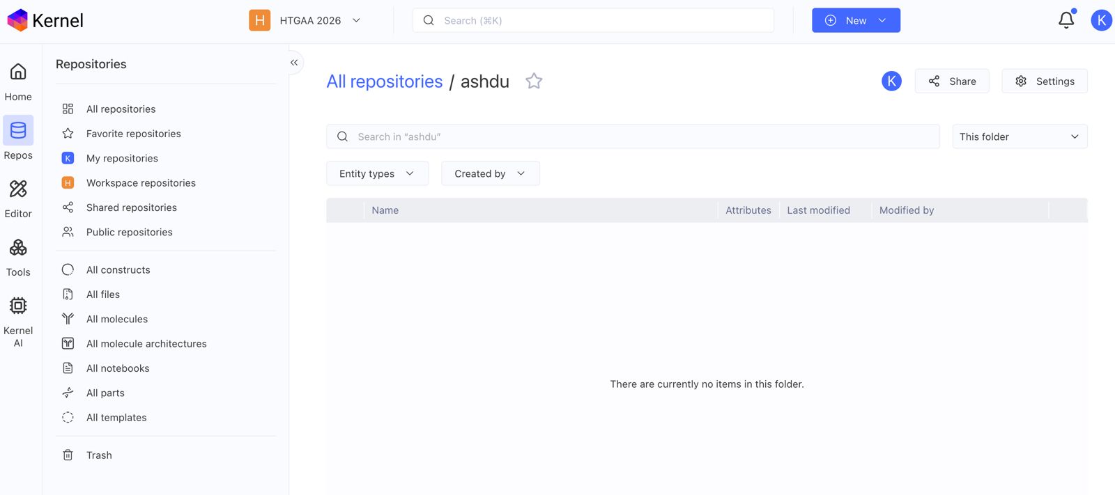
Create a blank Notebook entry to document the homework and save it to that Repository
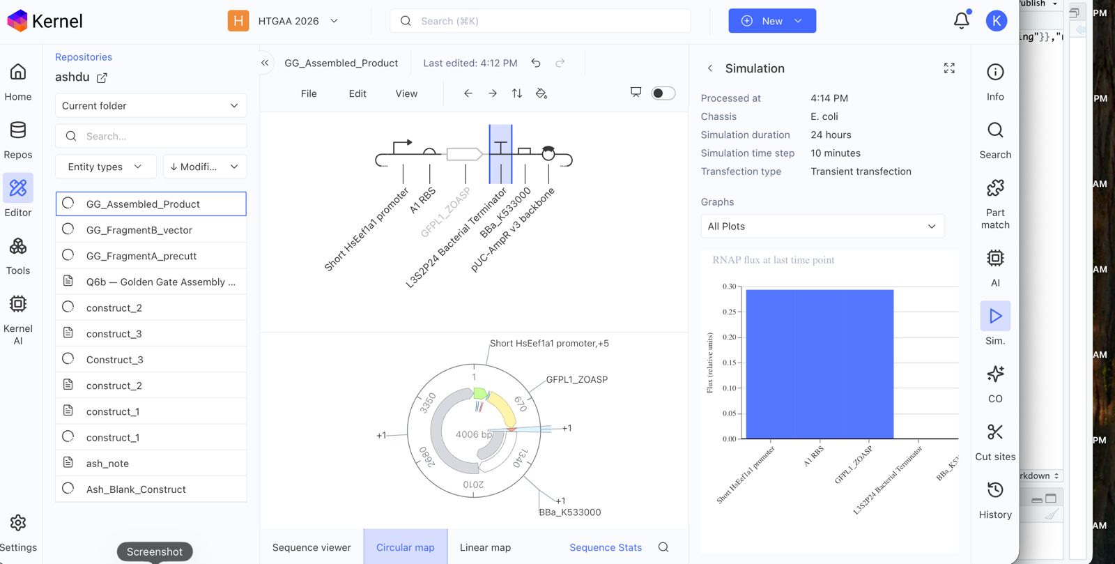
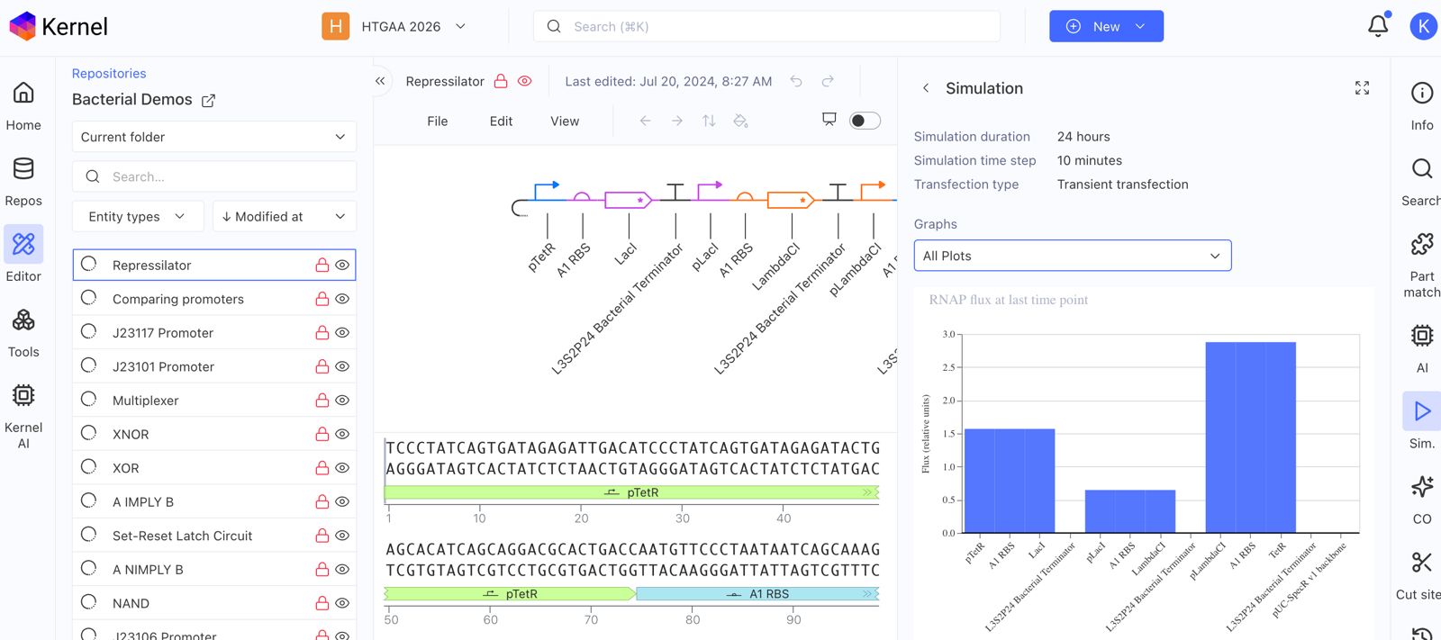
Explore the devices in the Bacterial Demos Repo to understand how the parts work together by running the Simulator on various examples, following the instructions for the simulator found in the “Info” panel (click the “i” icon on the right to open the Info panel)
Create a blank Construct and save it to your Repository
Recreate the Repressilator in that empty Construct by using parts from the Characterized Bacterial Parts repository
Search the parts using the Search function in the right menu
Drag and drop the parts into the Construct
Confirm it works as expected by running the Simulator (“play” button) and compare your results with the Repressilator Construct found in the Bacterial Demos repository
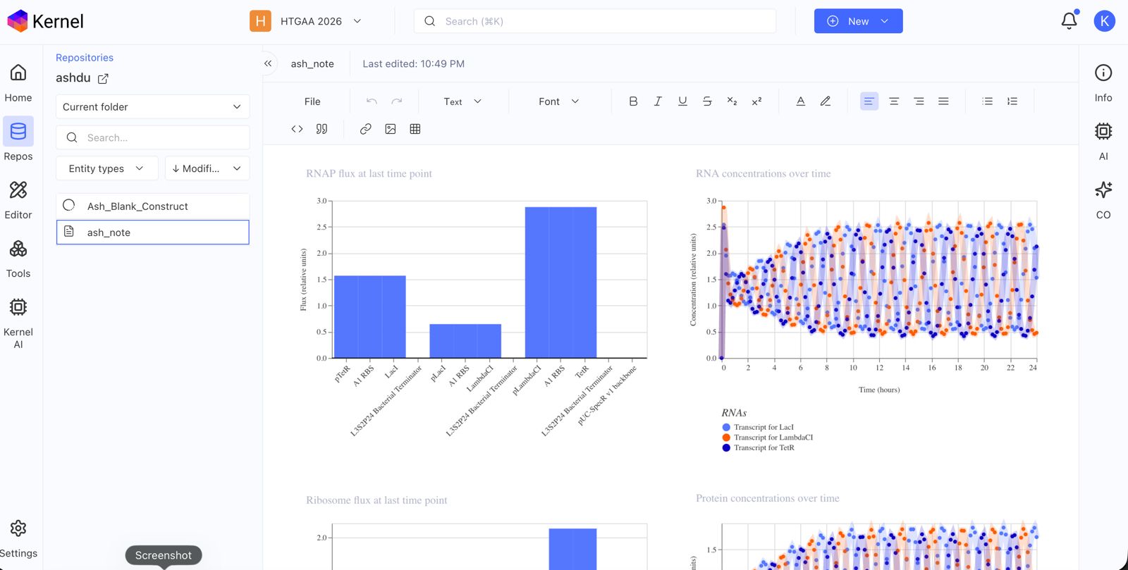
Document all of this work in your Notebook entry - you can copy the glyph image and the simulator graphs, and paste them into your Notebook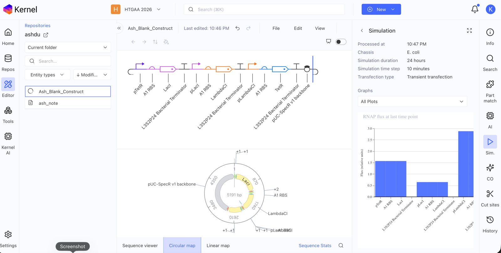
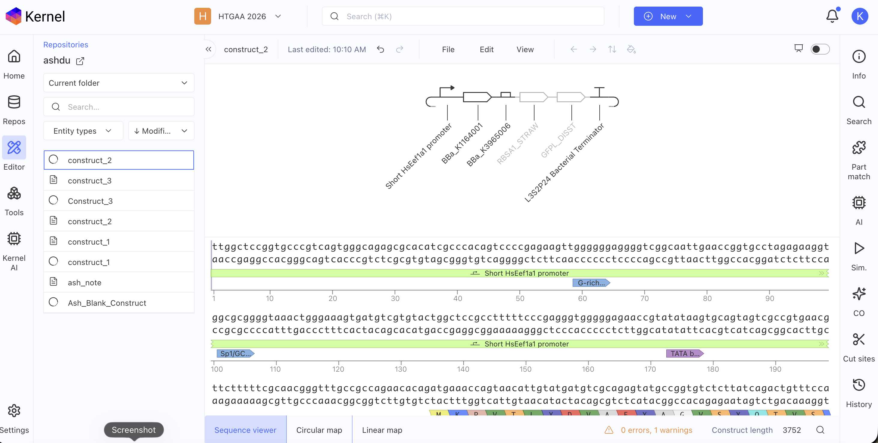
Build three of your own Constructs using the parts in the Characterized Bacterials Parts Repo
Explain in the Notebook Entry how you think each of the Constructs should function
Run the simulator and share your results in the Notebook Entry
If the results don’t match your expectations, speculate on why and see if you can adjust the simulator settings to get the expected outcome

What advantages do IANNs have over traditional genetic circuits, whose input/output behaviors are Boolean functions?
Traditional genetic circuits operate as Boolean logic gates: they classify inputs as either “on” (1) or “off” (0) and produce outputs that are likewise binary. While this is powerful for implementing discrete decisions — such as activating a kill switch if and only if two specific signals are simultaneously present — Boolean circuits are fundamentally limited in their ability to process the continuous, graded molecular signals that characterise real biological environments. Intracellular concentrations of transcription factors, metabolites, and signalling molecules are not naturally binary; they span continuous ranges that carry information that a simple Boolean threshold necessarily discards.
IANNs overcome this limitation by implementing analog computation, in which each molecular “neuron” computes a weighted sum of its continuous-valued inputs, passes that sum through a nonlinear activation function, and produces a graded output that can itself serve as an input to the next layer. This architecture enables a single engineered cell to perform multi-threshold classification — distinguishing not just “signal present” from “signal absent” but grading responses proportionally to signal intensity, and separating input patterns that no Boolean gate could resolve without an exponentially larger circuit. For example, a cell expressing a two-input biomolecular perceptron can draw a separating hyperplane in the continuous input space of two molecular concentrations, classifying cell states that would require many cascaded Boolean gates to approximate.
A second key advantage is graceful degradation under noise: because IANNs operate over a continuous input range, they can be designed with soft thresholds that smooth over stochastic fluctuations in molecule numbers — a pervasive problem in cells, where copy numbers of regulatory molecules are often in the tens to hundreds range. Boolean gates, which depend on crossing a hard threshold, are comparatively fragile to such noise. Third, IANNs are in principle extendable toward online learning, in which the synaptic weights (encoded by molecular concentrations or binding affinities) can be updated as a function of experience — an entirely alien concept to hardwired Boolean logic. Taken together, IANNs expand the computational vocabulary available to synthetic biology from a finite set of logic operations to a continuous, composable, and theoretically universal function approximation framework.
Describe a useful application for an IANN; include a detailed description of input/output behavior, as well as any limitations an IANN might face to achieve your goal.
One compelling application for an IANN is the continuous intracellular monitoring and correction of iron overload in patients with hereditary hemochromatosis — a genetic disorder characterised by excessive gastrointestinal absorption of dietary iron, leading to toxic iron deposition in the liver, heart, and pancreas. Current treatment requires regular phlebotomy, which is effective but burdensome and cannot respond dynamically to real-time fluctuations in free labile iron. An IANN-based therapeutic cell (for example, an engineered hepatocyte or gut epithelial cell) could be designed as follows. Two inputs are presented to a single-layer intracellular perceptron:
X₁: the intracellular concentration of labile iron pool (LIP), sensed indirectly via an iron-responsive element (IRE)–iron regulatory protein (IRP) system, which naturally controls mRNA translation in proportion to free iron levels. A synthetic construct could link IRP binding to the transcription or translation of an intermediate regulatory RNA, converting iron concentration into a molecular signal. X₂: a constitutive bias input (a fixed-level transcript) that sets the activation threshold — encoding the notion that the circuit should only respond when iron exceeds a safe baseline, analogous to a bias unit in a standard perceptron.
The perceptron computes the weighted sum of these inputs. When the weighted iron signal exceeds the threshold set by the bias, the activation function triggers expression of the output gene: a codon-optimised ferritin heavy-chain transgene, which sequesters excess free iron into inert ferritin complexes and prevents cellular damage. The output is graded — the more the iron concentration exceeds the threshold, the more ferritin is produced — in contrast to a Boolean circuit, which would either produce a fixed amount of ferritin or none at all, regardless of the severity of iron overload. Several important limitations must be acknowledged. First, IANNs currently cannot perform online weight adjustment in living cells at the speed required for therapeutic use; weights are set at the time of circuit design and cannot recalibrate if the patient’s physiology changes. Second, the molecular components encoding the perceptron — endoribonucleases, regulatory RNA hairpins, sequestration species — impose a metabolic burden on the host cell, and this burden grows with the complexity of the network, potentially impairing normal cellular function. Third, molecular noise in cells means that the effective threshold may drift over time as component concentrations fluctuate, making it difficult to guarantee that the circuit reliably distinguishes pathological from physiological iron levels. Fourth, an in vivo implementation raises significant immunogenicity concerns: the endoribonuclease components (e.g., Csy4, which originates from Pseudomonas aeruginosa) could trigger immune responses in a human host. These limitations suggest that near-term applications of IANNs may be better suited to ex vivo cell engineering or biosensor contexts rather than direct in vivo therapeutics.
Below is a diagram depicting an intracellular single-layer perceptron where the X1 input is DNA encoding for the Csy4 endoribonuclease and the X2 input is DNA encoding for a fluorescent protein output whose mRNA is regulated by Csy4. Tx: transcription; Tl: translation.
Draw a diagram for an intracellular multilayer perceptron where layer 1 outputs an endoribonuclease that regulates a fluorescent protein output in layer 2.

Fungal materials — chiefly derived from mycelium, the vegetative network of interwoven hyphae produced by filamentous fungi — have been commercialised across several industries over the past decade. The most mature application is mycelium-based composite packaging (e.g., Ecovative Design’s Mushroom® Packaging), in which agricultural waste such as corn husks or hemp hurds is inoculated with fungal spores, allowed to colonise and bind the substrate, then heat-killed and dried to produce a rigid, foam-like material used in place of expanded polystyrene for protective packaging. A second prominent category is myco-leather: pure mycelium mats produced by companies such as Bolt Threads (Mylo™) and MycoWorks (Reishi™) are processed into flexible sheets resembling animal leather and have been used in fashion accessories, including a limited-edition Hermès handbag. Third, mycoprotein — most famously Quorn, derived from Fusarium venenatum — has been on the market since the 1980s as a high-protein, meat-substitute food ingredient. More nascent applications include mycelium-based thermal insulation panels, biocement for construction, and even flexible electronic substrates exploiting the high conductivity of processed mycelium films.
The advantages of mycelium materials over their conventional counterparts are substantial. They are fully biodegradable, decomposing within weeks to months under composting conditions, in contrast to expanded polystyrene (which persists for ~50 years) or synthetic leather (derived from petroleum-based polyurethane). They can be grown on agricultural waste and byproducts — low-cost, abundant feedstocks — requiring no petroleum inputs, which reduces their carbon footprint relative to synthetic foam and plastic alternatives. They are mouldable during growth, meaning complex three-dimensional shapes can be formed without energy-intensive casting or machining. For myco-leather specifically, production avoids the toxic tanning chemicals and greenhouse gas emissions associated with conventional livestock-based leather.
The disadvantages are equally significant and should not be understated. Mycelium composites typically exhibit lower and less consistent mechanical properties than synthetic analogues: their tensile strength, compressive modulus, and moisture resistance vary substantially with fungal species, substrate composition, and growth conditions, making quality control challenging at industrial scale. High moisture absorption is a persistent problem — mycelium-based foams can absorb significant water, compromising their insulating and structural properties in humid environments. Biodegradability, while an environmental advantage, is simultaneously a durability disadvantage: myco-leather goods will degrade under prolonged exposure to moisture, UV light, or biological activity at rates that animal leather or synthetic leather would not. Finally, scaling production while maintaining consistent properties and sterility is technically demanding and costly, and life-cycle assessments suggest that the energy inputs for controlled fungal cultivation can partially offset the environmental benefits, particularly where renewable energy is not available .
One application I find particularly compelling is engineering filamentous fungi for targeted heavy-metal bioremediation — specifically, the removal of cadmium, lead, and arsenic from contaminated soils and industrial wastewater. Wild-type fungi already exhibit some capacity for metal biosorption via their cell walls, but this is passive and non-selective. I would want to genetically engineer a species such as Aspergillus niger or Trichoderma reesei to overexpress metallothioneins (small cysteine-rich metal-binding proteins) and ABC-type metal transporters that actively import toxic metals into vacuoles, concentrating them intracellularly for subsequent extraction by harvesting the mycelium rather than using energy-intensive chemical treatments. A second engineering goal would be to add a biosensor output — for instance, linking metal accumulation to the expression of a fluorescent reporter — so that the mycelium itself signals when remediation capacity is saturated and biomass needs to be replaced. This is precisely the kind of continuous, graded signal-response behaviour that an IANN architecture (from Part 1) could implement.
There are several compelling advantages of performing this synthetic biology in fungi rather than bacteria. First, fungi are eukaryotes, meaning they possess the post-translational modification machinery — N-linked glycosylation, disulfide bond formation, proper protein folding in the endoplasmic reticulum — required to produce complex proteins such as metallothioneins and secreted enzymes in their active forms; many such proteins are misfolded or inactive when expressed in E. coli. Second, filamentous fungi grow as mycelial networks that can extend through soil, bridging air-liquid interfaces and penetrating into pore spaces inaccessible to bacterial biofilms — a critical advantage for in situ bioremediation, where the contaminant is spatially distributed and often in a partly air-filled matrix. Third, many filamentous fungi are GRAS-status organisms (Generally Recognised As Safe), reducing regulatory barriers for environmental release relative to engineered bacteria, some of which carry biosafety concerns. Fourth, fungi have extraordinary metabolic versatility: they can catabolise lignin, cellulose, and xenobiotic compounds via oxidative enzymes (laccases, peroxidases) that are absent from most bacteria, making them uniquely suited to environments contaminated with both heavy metals and complex organic pollutants simultaneously. Finally, the physical scaffold of mycelium itself has structural utility — a bioremediation mycelium network can be harvested as a solid biomass enriched in bound metals, rather than requiring centrifugation or filtration of a bacterial cell suspension, simplifying downstream metal recovery.
A counter-consideration is that fungal genetic engineering has historically been more technically challenging than in bacteria, due to lower rates of homologous recombination in many species and the relative scarcity of validated synthetic promoters and genetic parts. However, the development of CRISPR-Cas9 tools adapted for Aspergillus and Trichoderma, alongside growing fungal parts registries, is rapidly closing this gap.
1. Explain the main advantages of cell-free protein synthesis over traditional in vivo methods, specifically in terms of flexibility and control over experimental variables. Name at least two cases where cell-free expression is more beneficial than cell production.
Cell-free protein synthesis (CFPS) offers a fundamentally different operating logic from in vivo expression: because there is no living cell to maintain, the reaction environment is open and directly accessible to the experimenter. This openness translates into three practical advantages. First, reaction components — amino acid concentrations, buffer conditions, redox potential, template concentration — can be tuned independently and in real time without the buffering effects of cellular homeostasis. Second, toxic proteins that would kill or arrest growing cells can be expressed freely in CFPS, since there is no cell viability to protect. Third, non-canonical amino acids, isotopic labels, or synthetic chemical groups can be incorporated site-specifically by supplementing the reaction directly, enabling protein engineering strategies that are impossible to sustain through the protein expression machinery of a living cell.
Two cases where cell-free expression is specifically more advantageous than cell-based production are: (1) membrane protein structural studies, where the absence of competing cellular membranes allows co-translational insertion directly into defined lipid nanodiscs of controlled composition, circumventing the protein aggregation and misfolding problems that arise during over-expression in intact cells; and (2) rapid on-demand diagnostic biosensors, where freeze-dried CFPS reactions can be deployed at the point of need without cold-chain infrastructure or biohazard containment — capabilities recently validated aboard the International Space Station.
2. Describe the main components of a cell-free expression system and explain the role of each component.
A cell-free expression system can be understood as a minimal reconstruction of the cellular central dogma pathway. The core components and their roles are as follows.
The DNA or mRNA template encodes the protein of interest and acts as the informational input; a strong promoter (e.g., T7) is typically used when a DNA template drives transcription. RNA polymerase (either endogenous in crude lysates or supplied purified as T7 RNAP in PURE systems) transcribes the DNA into mRNA. The ribosome is the catalytic core of translation, reading the mRNA and elongating the polypeptide chain with the assistance of elongation factors (EF-Tu, EF-G) and initiation/release factors; roughly 4 ATP equivalents are consumed per peptide bond formed. Aminoacyl-tRNA synthetases (aaRSs) charge each of the 20 tRNAs with their cognate amino acid, and tRNA molecules deliver those charged amino acids to the ribosome A-site. Amino acids serve as the building block pool; depletion of the amino acid pool is one of the primary causes of reaction stalling in crude lysate systems. The energy regeneration module — commonly phosphoenolpyruvate (PEP) plus pyruvate kinase, creatine phosphate plus creatine kinase, or 3-phosphoglycerate (3-PGA) — continuously regenerates ATP and GTP from ADP/GDP to sustain translation. Magnesium ions are essential cofactors for ribosome function and nucleotide-dependent enzymes; their concentration must be carefully titrated. Potassium ions set the ionic environment required for ribosome activity. Finally, polyethylene glycol (PEG) or similar crowding agents mimic the macromolecular crowding of the cytoplasm and can improve translation efficiency. In the PURE system, all these components are defined and provided as purified proteins, offering reproducibility and the absence of contaminating nucleases and proteases.
3. Why is energy provision regeneration critical in cell-free systems? Describe a method you could use to ensure continuous ATP supply in your cell-free experiment.
Energy regeneration is critical in CFPS because translation is an inherently ATP- and GTP-intensive process — approximately 4 high-energy phosphate equivalents are consumed per amino acid incorporated (2 ATP for aminoacyl-tRNA charging, 1 GTP for tRNA delivery to the ribosome, and 1 GTP for translocation) (Jewett & Swartz, 2004). Without continuous regeneration, the ATP pool is rapidly depleted, causing translation to stall. A further complication is the accumulation of inorganic phosphate (Pi) as a byproduct of phosphotransfer reactions: elevated Pi sequesters Mg²⁺, which is an essential ribosomal cofactor, thereby inhibiting both transcription and translation. An effective energy system must therefore not only regenerate ATP but also limit Pi accumulation (Calhoun & Swartz, 2007).
One reliable method is the 3-phosphoglycerate (3-PGA) system, in which 3-PGA enters a truncated glycolytic pathway to regenerate ATP while producing only pyruvate and acetate as by-products — neither of which chelates Mg²⁺ appreciably. Studies have shown that 3-PGA-powered CFPS sustains reactions for several hours and achieves yields exceeding 1 mg/mL of recombinant protein (Kim & Swartz, 2001). A complementary strategy is to use a fed-batch or semi-continuous dialysis reactor format, in which fresh substrates (ATP precursors, amino acids, cofactors) are continuously exchanged into the reaction while inhibitory by-products are dialysed out, extending productive synthesis from hours to potentially days (Spirin et al., 1988). For classroom or field-deployable settings, the simpler creatine phosphate / creatine kinase (CP/CK) system remains widely used, despite the 1:1 stoichiometric phosphate release it entails, because of its low cost and ease of formulation.
4. Compare prokaryotic versus eukaryotic cell-free expression systems. Choose a protein to produce in each system and explain why.
Prokaryotic CFPS systems — most commonly derived from E. coli lysates — are fast to prepare, inexpensive, highly productive (yields of 1–4 mg/mL are achievable in optimised formats), and compatible with a wide range of T7-based expression vectors. Their principal limitation is the absence of the eukaryotic post-translational modification machinery: E. coli extracts cannot perform N-linked glycosylation, and the reducing cytoplasmic environment is unfavourable for the formation of disulfide bonds, which are essential for many human therapeutic proteins. Eukaryotic CFPS systems — including wheat germ extract (WGE), rabbit reticulocyte lysate (RRL), and Chinese hamster ovary (CHO) cell lysates — provide access to chaperones, signal recognition particles, and post-translational processing machinery that support proper folding of complex human proteins. They tend to be slower and more expensive than prokaryotic systems, but are indispensable when the target protein requires glycosylation, specific disulfide connectivity, or processing by signal peptidase.
For the prokaryotic system (E. coli extract), an excellent choice is single-chain variable fragment (scFv) antibody, a small (~27 kDa) recombinant antibody format that does not require glycosylation and whose binding function can be verified rapidly by an ELISA-based assay. The fast turnaround of bacterial CFPS (reactions complete within 4–6 hours) is ideal for iterative screening of antibody variants during affinity maturation campaigns.
For the eukaryotic system (CHO or insect cell extract), erythropoietin (EPO) is the appropriate choice. EPO is a 165-amino acid glycoprotein hormone in which three N-linked and one O-linked glycan chains account for approximately 40% of its molecular weight and are critical for its in vivo half-life and receptor-binding activity. Expressing EPO in a prokaryotic system yields aglycosylated protein with substantially reduced biological activity; a CHO-based CFPS system that includes microsomes or glycosylation enzymes can produce a glycoform closer to the therapeutic molecule.
5. How would you design a cell-free experiment to optimize the expression of a membrane protein? Discuss the challenges and how you would address them in your setup.
Membrane proteins (MPs) represent the most challenging class of targets for CFPS because their hydrophobic transmembrane domains are insoluble in aqueous solution: without a lipid environment, they aggregate irreversibly into inclusion body-like precipitates immediately after synthesis. A well-designed cell-free membrane protein experiment must therefore couple protein synthesis to a compatible hydrophobic scaffold present in the reaction from the outset.
The recommended strategy is co-translational insertion into pre-formed nanodiscs. Nanodiscs are discoidal phospholipid bilayer patches stabilised by an amphipathic membrane scaffold protein (MSP); their diameter (~10 nm) and lipid composition can be controlled precisely. By including nanodiscs at optimised concentrations (typically 0.2–2 mg/mL) in the CFPS reaction, the nascent transmembrane protein can fold co-translationally into the bilayer rather than encountering aqueous solution at all, preserving its native fold and function. Studies have shown that nanodisc-based CFPS supports correct folding of GPCRs, ion channels, and multi-pass transporters at yields sufficient for structural studies by NMR or cryo-EM.
Three specific challenges and how to address them: (1) Aggregation during synthesis — mitigated by using lipid nanodiscs as described above, supplemented if needed with detergents at sub-CMC concentrations such as Brij-35 to stabilise partially-folded intermediates; (2) Low expression yield — membrane proteins are often toxic in in-vivo systems but in CFPS this is no constraint; yield can be maximised by optimising the concentration of nanodiscs, adjusting Mg²⁺ levels (often 10–14 mM for membrane protein CFPS rather than the standard 8–10 mM), and screening N-terminal fusion tags to improve ribosome engagement; (3) Verification of correct folding — since Western blotting confirms synthesis but not function, activity assays (e.g., ligand binding ELISA for GPCRs, patch-clamp for channels) or limited proteolysis footprinting should be used to confirm the protein has adopted its native architecture.
6. Imagine you observe a low yield of your target protein in a cell-free system. Describe three possible reasons for this and suggest a troubleshooting strategy for each.
Low yield in a CFPS reaction can arise at multiple points in the expression pathway. Here are three common causes and their corresponding troubleshooting strategies.
Reason 1 — Premature energy depletion and ATP starvation. If the energy regeneration system is insufficient or the secondary energy source (e.g., phosphoenolpyruvate) is consumed too quickly, ATP levels drop below the threshold required to sustain elongation, causing ribosomes to stall prematurely. The troubleshooting strategy is to measure the reaction’s pH over time using a microelectrode or pH-sensitive dye (acidification indicates Pi accumulation and ATP exhaustion) and to switch to a more sustained energy substrate such as 3-PGA, which produces less Pi per ATP regenerated, or to implement a fed-batch format with controlled substrate addition.
Reason 2 — mRNA instability and degradation. Crude cell extracts contain residual ribonucleases that can degrade the mRNA template, especially if it lacks a strong 5’ untranslated region (UTR), a stable secondary structure at the 3’ end, or is not capped in eukaryotic systems. The troubleshooting strategy is to run the reaction without protein expression template and assess background RNase activity using a fluorescent RNA reporter; if high, add RNase inhibitor (e.g., RNasin), switch to a DNA template with a strong ribosome binding site, or use a PURE system that is free of nucleases.
Reason 3 — Suboptimal magnesium and potassium ion concentrations. Both Mg²⁺ and K⁺ profoundly affect ribosome assembly and activity, and their optimal concentrations depend on the extract lot, target protein, and energy system used. A single mM deviation in [Mg²⁺] can halve protein yield. The troubleshooting strategy is to perform a systematic two-dimensional titration of Mg²⁺ (range: 4–16 mM) and K⁺ (range: 60–200 mM) against protein yield measured by fluorescence (if GFP is used as a reporter) or SDS-PAGE densitometry, and re-optimise for each new extract batch or protein target.
Design an example of a useful synthetic minimal cell as follows:
Pick a function and describe it.
a. What would your synthetic cell do? What is the input and what is the output?
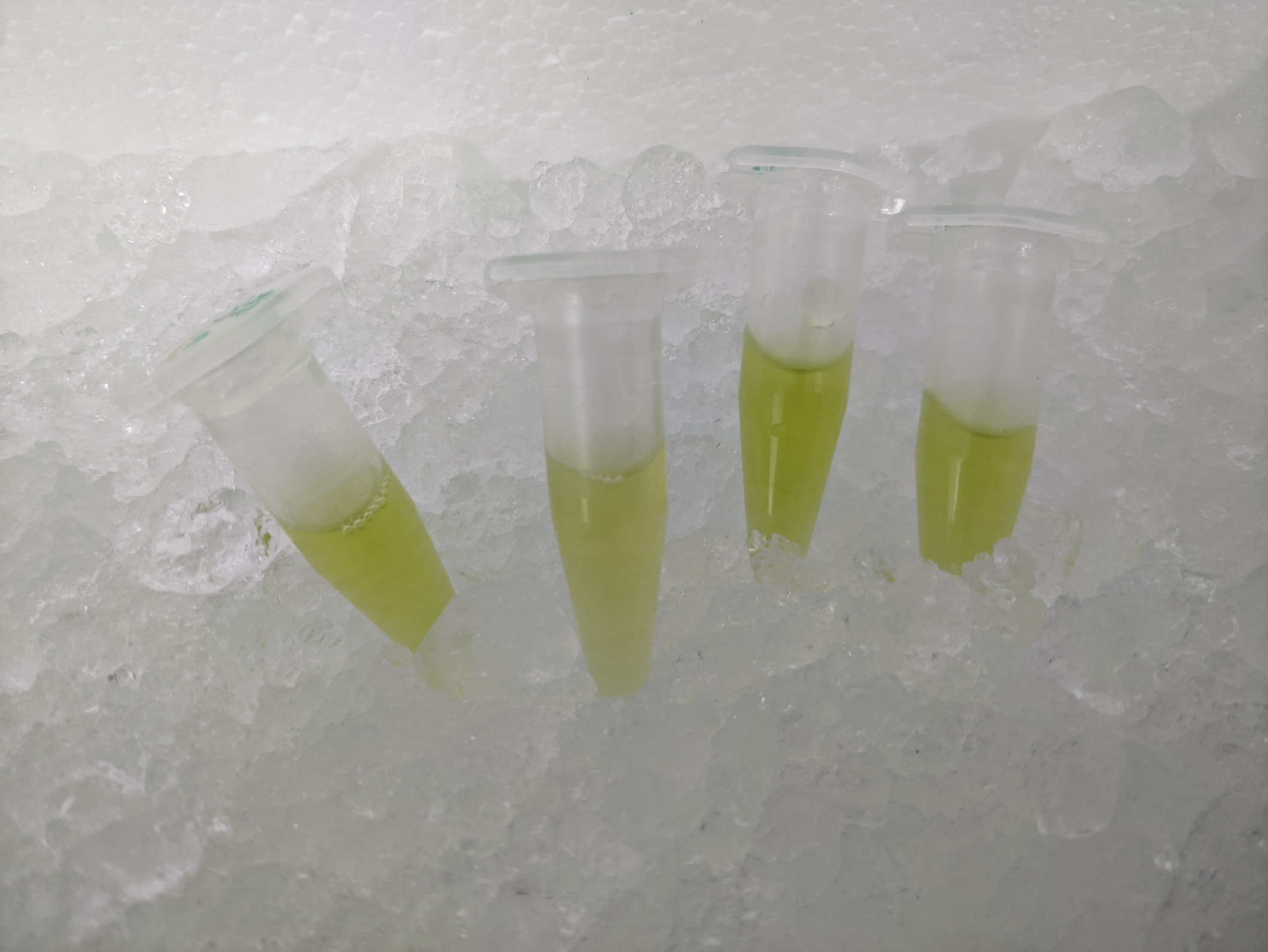
The proposed synthetic minimal cell (SMC) functions as a field-deployable water quality sensor for antibiotic resistance. The input is the presence of beta-lactam antibiotic residues (specifically ampicillin) in environmental water samples, detected via a riboswitch aptamer domain that undergoes a conformational change upon ligand binding. The output is fluorescent GFP produced by the encapsulated CFPS system, reportable visually with a handheld fluorescence viewer such as the miniPCR P51 Molecular Fluorescence Viewer.
b. Could this function be realized by cell-free Tx/Tl alone, without encapsulation?
No. Encapsulation is essential for two reasons: first, the lipid membrane creates a concentration gradient that amplifies the input signal — only molecules that enter or diffuse across the bilayer trigger the sensor, reducing false positives from trace non-specific binding. Second, the membrane physically separates the CFPS machinery from environmental nucleases and proteases present in raw water samples, which would otherwise degrade the RNA aptamer and mRNA templates. Without encapsulation, the reaction would be rapidly inactivated in complex environmental matrices.
c. Could this function be realized by genetically modified natural cell?
Yes, in principle: an E. coli strain engineered with an ampicillin-responsive transcription factor driving GFP expression could detect beta-lactams. However, release of live GMO bacteria into environmental water samples raises serious biosafety and ecological concerns, and the engineered organism may not survive or function predictably in the field. The SMC offers a fully abiotic, self-contained, containable alternative with no replication capacity.
d. Describe the desired outcome of your synthetic cell operation.
In the presence of ampicillin above a defined threshold concentration (~10 µM), the riboswitch aptamer within the SMC adopts its ligand-bound conformation, allowing ribosomal readthrough of an upstream inhibitory sequence and enabling translation of the GFP reporter. The operator observes green fluorescence from the SMC population when viewed under blue LED excitation — a simple positive/negative readout of water contamination.
Design all components that would need to be part of your synthetic cell.
a. What would be the membrane made of?
POPC (1-palmitoyl-2-oleoyl-sn-glycero-3-phosphocholine) as the primary structural lipid, with 10 mol% POPG (1-palmitoyl-2-oleoyl-sn-glycero-3-phospho-(1’-rac-glycerol)) to introduce a slight anionic character that improves vesicle stability and reduces aggregation. No cholesterol is required for this room-temperature sensor application.
b. What would you encapsulate inside? Enzymes, small molecules.
A bacterial cell-free Tx/Tl system (E. coli S30 extract), the riboswitch-GFP DNA construct, an ATP regeneration module (creatine phosphate + creatine kinase), all 20 amino acids, NTPs, Mg²⁺, and K⁺ at optimised concentrations.
c. Which organism your Tx/Tl system will come from? Is bacterial OK, or do you need a mammalian system for some reason? (hint: for example, if you want to use small molecule modulated promotors, like Tet-ON, you need mammalian)
Bacterial (E. coli S30 extract), because the riboswitch is derived from a prokaryotic aptazyme architecture and functions via modulation of ribosome access to the Shine-Dalgarno sequence — a mechanism specific to bacterial translation.
d. How will your synthetic cell communicate with the environment? (hint: are substrates permeable? or do you need to express the membrane channel?)
Ampicillin is a small, moderately amphipathic beta-lactam molecule (~349 Da) that can passively permeate phospholipid bilayers to a limited but measurable extent. At the ampicillin concentrations relevant for contamination detection (10–100 µM), passive permeation is sufficient to trigger the internal riboswitch without requiring an active transporter. GFP output remains internal and is detected non-destructively by fluorescence spectroscopy or imaging.
Experimental details
a. List all lipids and genes. (bonus: find the specific genes; for example, instead of just saying “small molecule membrane channel” pick the actual gene.)
Lipids: POPC (Avanti Polar Lipids #850457), POPG (Avanti Polar Lipids #840457)
Genes: Ampicillin-responsive riboswitch–GFP fusion: a synthetic construct encoding an engineered aptazyme responsive to beta-lactams (based on the aptazyme architecture of Wieland & Hartig, 2008) fused upstream of a GFP ORF under a T7 promoter
Specific gene-GFP variant: sfGFP (superfolder GFP; Addgene plasmid #54579), chosen for its robust folding kinetics in cell-free systems
b. How will you measure the function of your system?
Measure GFP fluorescence of the SMC suspension using a plate reader (excitation 488 nm, emission 510 nm) or a P51 handheld viewer for field deployment. A positive control containing a constitutively expressed GFP plasmid and a negative control of vesicles containing a scrambled riboswitch should bracket every experiment. Vesicle integrity is confirmed by dynamic light scattering (DLS) before and after the assay.
Freeze-dried cell-free systems can be incorporated into all kinds of materials as biological sensors or as inducible enzymes to modify the material itself or the surrounding environment. Choose one application field — Architecture, Textiles/Fashion, or Robotics — and propose an application using cell-free systems that are functionally integrated into the material. Answer each of these key questions for your proposal pitch:
Write a one-sentence summary pitch sentence describing your concept.
A freeze-dried cell-free biosensor woven directly into a protective work garment that changes from orange to green fluorescence within 90 minutes of contact with airborne organophosphate pesticide residues, providing farm workers with a passive, wearable early-warning system for chemical exposure.
How will the idea work, in more detail? Write 3-4 sentences or more.
The garment integrates freeze-dried cell-free (FDCF) synthetic biology circuits embedded in cellulose-based reaction insets woven into the chest panel of the fabric, using the methodology developed by Nguyen, Soenksen et al. The FDCF reaction encodes an organophosphate-responsive genetic circuit: acetylcholinesterase (AChE) activity is coupled to a split-reporter system such that AChE inhibition by organophosphates — detectable at concentrations as low as 10 nM — derepresses expression of a fluorescent aptamer. A polymeric optical fibre network interwoven with the fabric continuously probes each reaction zone for changes in fluorescence (orange baseline → green signal-positive), and the output is transmitted via Bluetooth to a paired smartphone application, alerting the wearer of exposure in real time. The reaction chambers are hermetically sealed and activated only by moisture — either sweat or rain — contacting the fibre insets, preventing premature activation during storage.
What societal challenge or market need will this address?
Organophosphate pesticide exposure is the leading cause of acute agricultural poisoning worldwide, responsible for an estimated 385 million cases of unintentional acute pesticide poisoning per year (WHO, 2019). Farm workers in low-to-middle income countries frequently lack access to personal air quality monitors or laboratory testing infrastructure. A textile-embedded FDCF sensor worn as ordinary work clothing would provide continuous, real-time, instrument-free exposure monitoring, enabling workers to evacuate contaminated areas before symptoms manifest and generating timestamped exposure logs usable in occupational health assessments.
How do you envision addressing the limitation of cell-free reactions (e.g., activation with water, stability, one-time use)?
The three primary limitations — activation with water, stability in humid environments, and one-time use — are addressed as follows. Activation by water is an inherent design feature here rather than a drawback: the sensor is intentionally triggered by sweat contact, and the fabric’s hydrophobic outer layer acts as a moisture gate, ensuring activation only after meaningful liquid contact. Long-term stability is achieved by lyophilising the CFPS reactions in the presence of trehalose as a cryoprotectant and sealing individual reaction zones in a vapour-barrier polymer matrix; prior work has demonstrated FDCF stability at ambient temperature for at least six months under these conditions. The single-use constraint is addressed architecturally: reaction zones are modular insets that can be removed and replaced by the wearer after each work day, analogous to replacing a spent filter cartridge, while the fibre optic network and smartphone interface are reusable across many cycles.
Freeze-dried cell-free reactions have great potential in space, where resources are constrained. As described in my talk, the Genes in Space competition challenges students to consider how biotechnology, including cell-free reactions, can be used to solve biological problems encountered in space. While the competition is limited to only high school students, your assignment will be to develop your own mock Genes in Space proposal to practice thinking about biotech applications in space!
For this particular assignment, your proposal is required to incorporate the BioBits® cell-free protein expression system, but you may also use the other tools in the Genes in Space toolkit (the miniPCR® thermal cycler and the P51 Molecular Fluorescence Viewer). For more inspiration, check out https://www.genesinspace.org/ .
1. Provide background information that describes the space biology question or challenge you propose to address. Explain why this topic is significant for humanity, relevant for space exploration, and scientifically interesting. (Maximum 100 words)
Galactic cosmic radiation (GCR) and solar energetic particles present a significant health risk during deep-space missions, inducing DNA double-strand breaks (DSBs) and oxidative base damage in astronaut cells. Current biomonitoring of radiation-induced DNA damage aboard the ISS requires blood draws, cryopreservation, and Earth-based laboratory analysis — an impractical pipeline for future lunar or Mars missions where resupply is impossible. Developing a rapid, portable, crew-operable assay for real-time radiation exposure biomonitoring is critical to protect astronaut health and to inform mission planning and shielding design for exploration beyond low-Earth orbit.
2. Name the molecular or genetic target that you propose to study. Examples of molecular targets include individual genes and proteins, DNA and RNA sequences, or broader -omics approaches. (Maximum 30 words) Target: p21 (CDKN1A) mRNA — a transcriptional target of the p53 DNA damage response pathway, reliably upregulated within hours of ionising radiation exposure in human cells.
3. Describe how your molecular or genetic target relates to the space biology question or challenge your proposal addresses. (Maximum 100 words)
When ionising radiation causes DNA DSBs, the tumour suppressor p53 is activated and drives transcription of p21/CDKN1A, a cyclin-dependent kinase inhibitor that halts the cell cycle to allow DNA repair. Because p21 mRNA accumulates in cells proportionally to the absorbed radiation dose, it is a well-validated molecular dosimeter. Importantly, p21 mRNA can be extracted from crew saliva or buccal cells — a non-invasive sample type fully compatible with spaceflight constraints — and detected using the BioBits® toehold switch platform without the need for PCR equipment or cold-chain reagents.
4. Clearly state your hypothesis or research goal and explain the reasoning behind it. (Maximum 150 words)
Hypothesis: BioBits®-based toehold switch sensors designed to detect human p21 mRNA will produce a fluorescent readout proportional to radiation dose, as measured in buccal cell RNA extracts collected from astronauts aboard the ISS, and will perform comparably to Earth-based qRT-PCR reference measurements.
Reasoning: Toehold switches — linear RNA hairpin structures that undergo conformational change upon hybridisation to a complementary trigger RNA — have been validated as highly sensitive, sequence-specific nucleic acid sensors in cell-free systems with detection limits as low as picomolar concentrations . Prior work by Kocalar et al. (2024) demonstrated that BioBits® performs robustly in microgravity. Because p21 mRNA is a human transcript expressed in cells easily obtainable by non-invasive buccal swab, the assay requires no genetic engineering of the crew, preserves biosafety, and is activatable by simple rehydration of the lyophilised BioBits® pellet with the extracted RNA sample.
5. Outline your experimental plan - identify the sample(s) you will test in your experiment, including any necessary controls, the type of data or measurements that will be collected, etc. (Maximum 100 words)
Samples: Buccal swabs collected from crew members at three time points — pre-mission baseline, 72 hours after a known solar energetic particle (SEP) event (using ISS radiation dosimetry logs as the reference), and at mission end. RNA is extracted using a portable lysis buffer compatible with the miniPCR kit.
Experiment: p21 toehold switch BioBits® reactions are rehydrated with crew RNA extract and incubated for 60 minutes at 37 °C. Fluorescence is read using the P51 Molecular Fluorescence Viewer; image intensity is quantified via the paired smartphone app.
Controls: Non-irradiated Earth buccal RNA (negative control); synthetic p21 mRNA spike-in (positive control); scrambled-sequence toehold switch (specificity control).
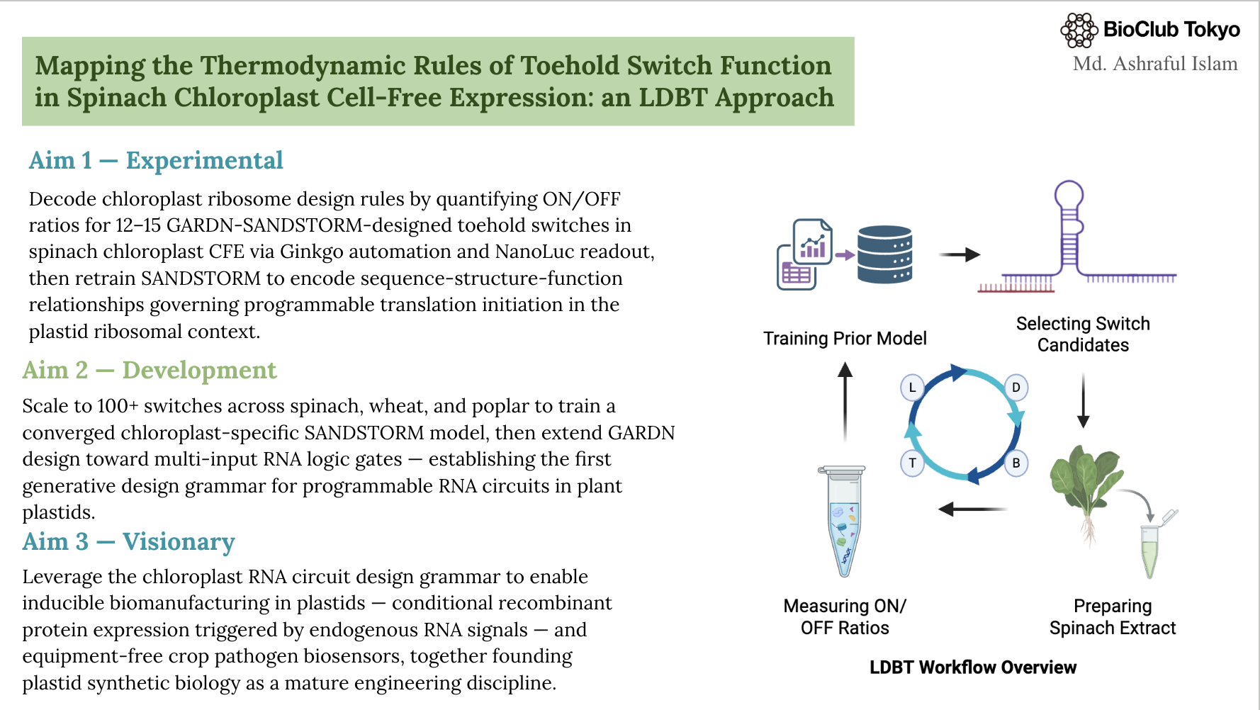
eGFP Sequence:
Based only on the predicted amino acid sequence of eGFP (see below), what is the calculated molecular weight? You can use an online calculator like the one here: https://web.expasy.org/compute_pi/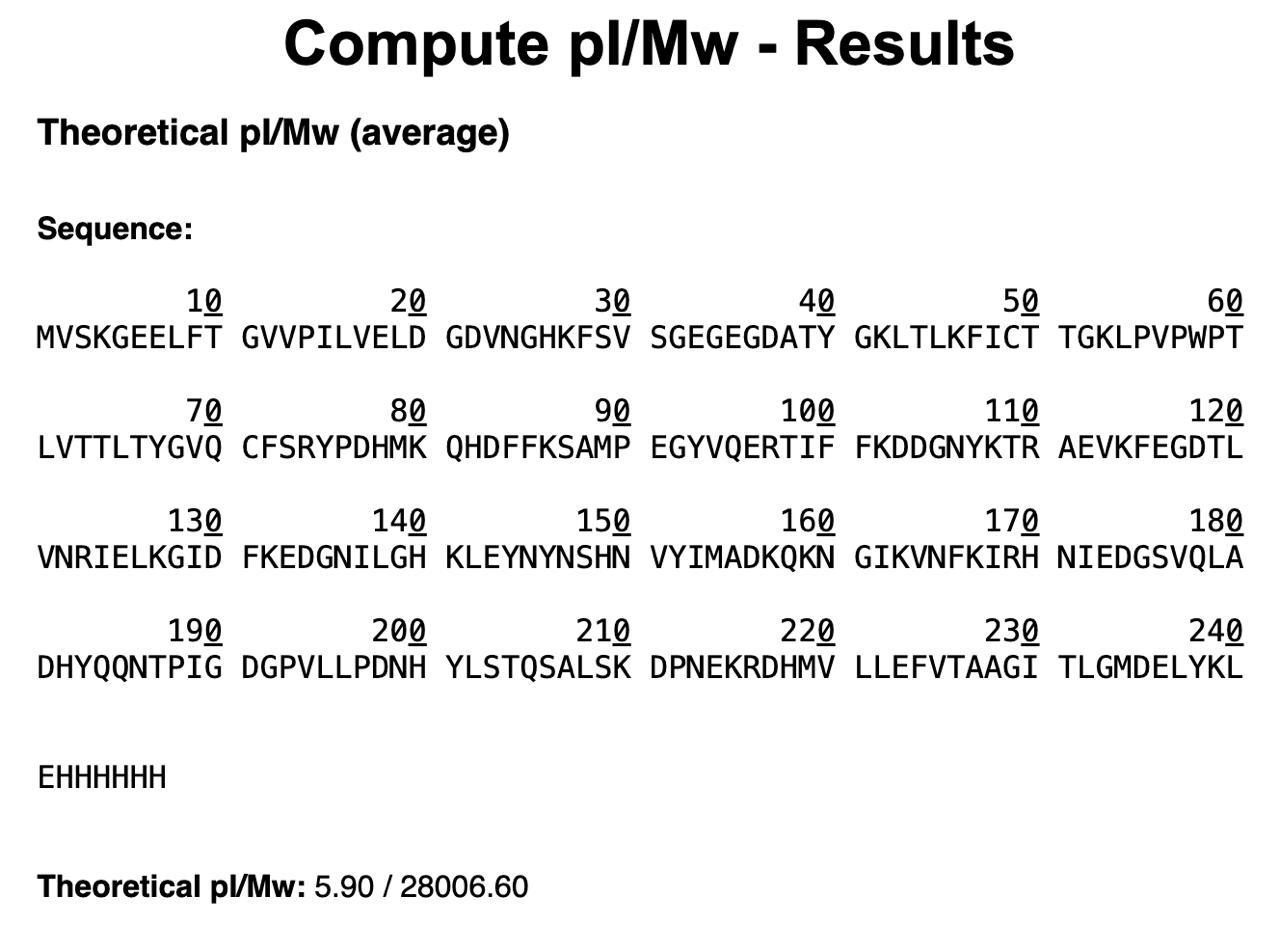
Calculate the molecular weight of the eGFP using the adjacent charge state approach described in the recitation. Select two charge states from the BioAccord data and:
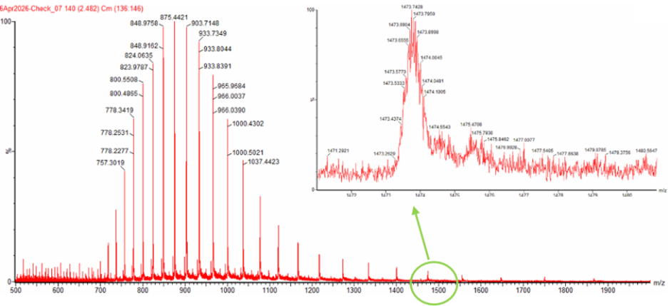 Figure 1. Mass Spectrum of intact eGFP protein from the Waters Xevo G3 LC-MS (a mass spectrometer with 30,000 resolution) with individual charge state peaks labeled with values.
Calculating $z$:
$$n = \frac{(m/z)_{n+1}}{(m/z)n - (m/z){n+1}}$$
$$n = \frac{875.4421}{903.7148 - 875.4421}$$
$$n = \frac{875.4421}{28.2727} = 30.963$$
We use the relationship between $m/z$, molecular weight ($M$), and charge ($z$):
$$M = z \times (m/z - H)$$
Peak 1 ($z = 31$): $$M = 31 \times (903.7148 - 1.007)$$ $$M = 31 \times 902.7078 = 27983.9418 \text{ Da}$$
Peak 2 ($z = 32$): $$M = 32 \times (875.4421 - 1.007)$$ $$M = 32 \times 874.4351 = 27981.9232 \text{ Da}$$
Average Molecular Weight ($M_{\text{avg}}$):
$$M_{\text{avg}} = \frac{27983.9418 + 27981.9232}{2} = 27982.9325 \text{ Da}$$
We use the deconvoluted average weight ($M_{\text{estimated}}$) and the predicted theoretical weight ($M_{\text{theoretical}}$).
Absolute Error: $$\text{Absolute Error} = 27982.9325 - 27875.41 = 107.5225 \text{ Da}$$
Relative Accuracy: $$\text{Accuracy} = \frac{|M_{\text{experiment}} - M_{\text{theoretical}}|}{M_{\text{theoretical}}}$$
$$\text{Accuracy} = \frac{107.5225}{27875.41} = 0.003858 \text{ (or } 0.386% \text{)}$$
We will digest the eGFP protein standard into peptides using trypsin (an enzyme that selectively cleaves the peptide bond after Lysine (K) and Arginine (R) residues. The resulting peptides will be analyzed on the Waters BioAccord LC-MS to measure their molecular weights and fragmented to confirm the amino acid sequence within each peptide – generating a “peptide map”. This process is used to confirm the primary structure of the protein.
There are a variety of tools available online to calculate protein molecular weight and predict a list of peptides generated from a tryptic digest. We will be using tools within the online resource Expasy (the bioinformatics resource portal of the Swiss Institute of Bioinformatics (SIB)) to predict a list of tryptic peptides from eGFP.
How many Lysines (K) and Arginines (R) are in eGFP? Please circle or highlight them in the eGFP sequence given in Waters Part I question 1 above. (Note: adding the sequence to Benchling as an amino acid file and clicking biochemical properties tab will show you a count for each amino acid).
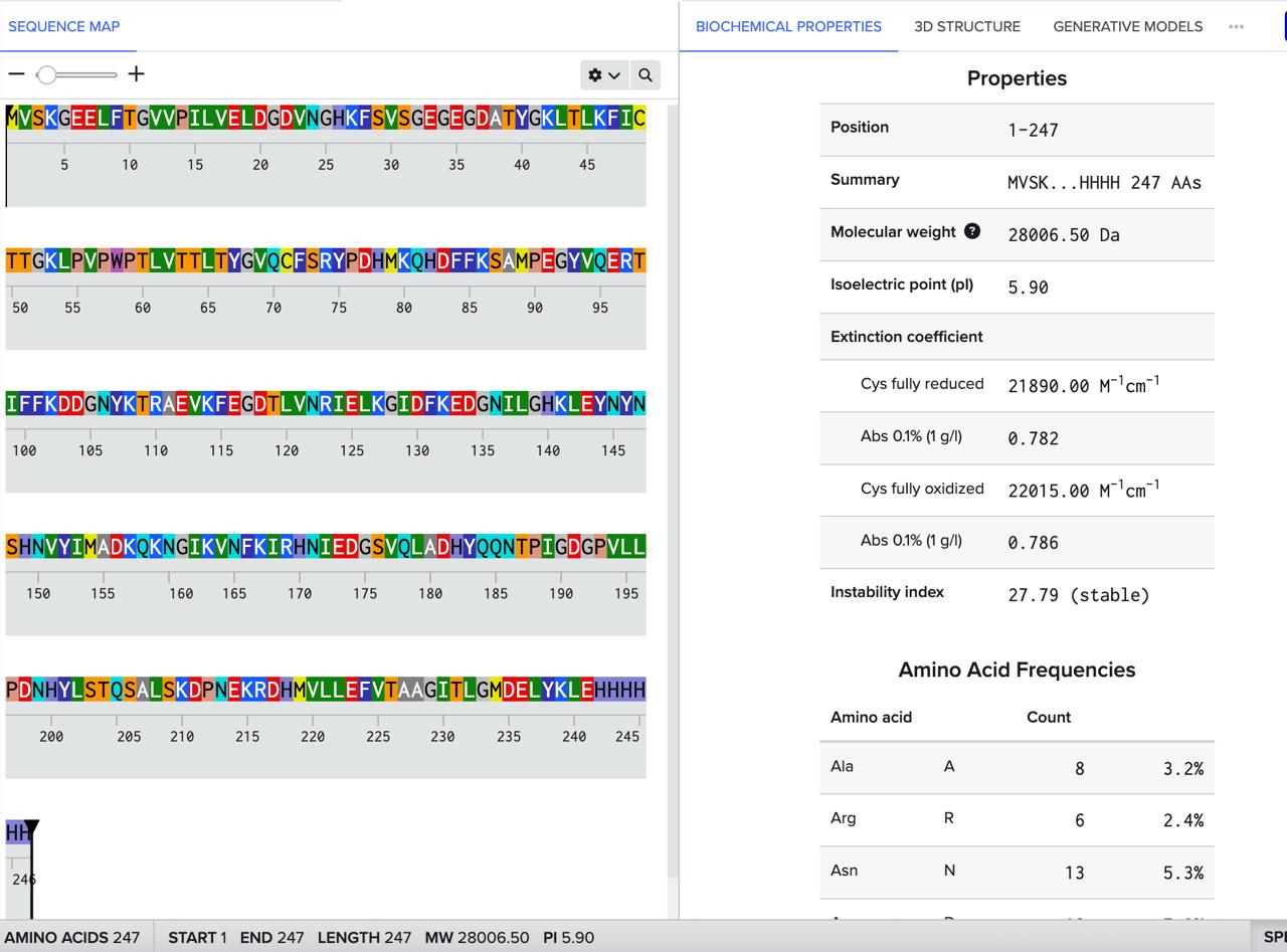
How many peptides will be generated from tryptic digestion of eGFP?
a. Navigate to https://web.expasy.org/peptide_mass/
b. Copy/paste the sequence above into the input box in the PeptideMass tool to generate expected list of peptides.
c. Use Figure 4 below as a guide for the relevant parameters to predict peptides from eGFP.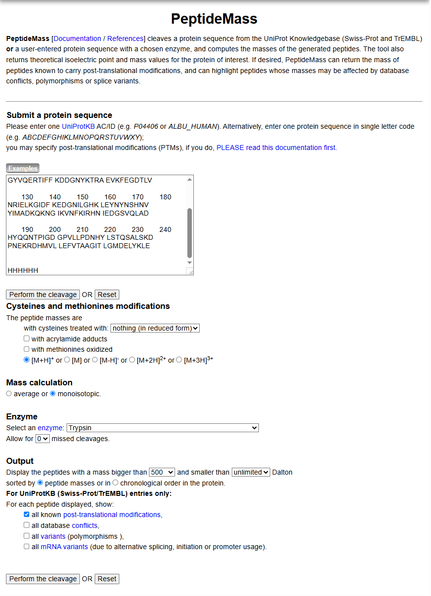
d. Click “Perform the Cleavage” button in the PeptideMass tool and report the number of peptides generated when using trypsin to perform the digest.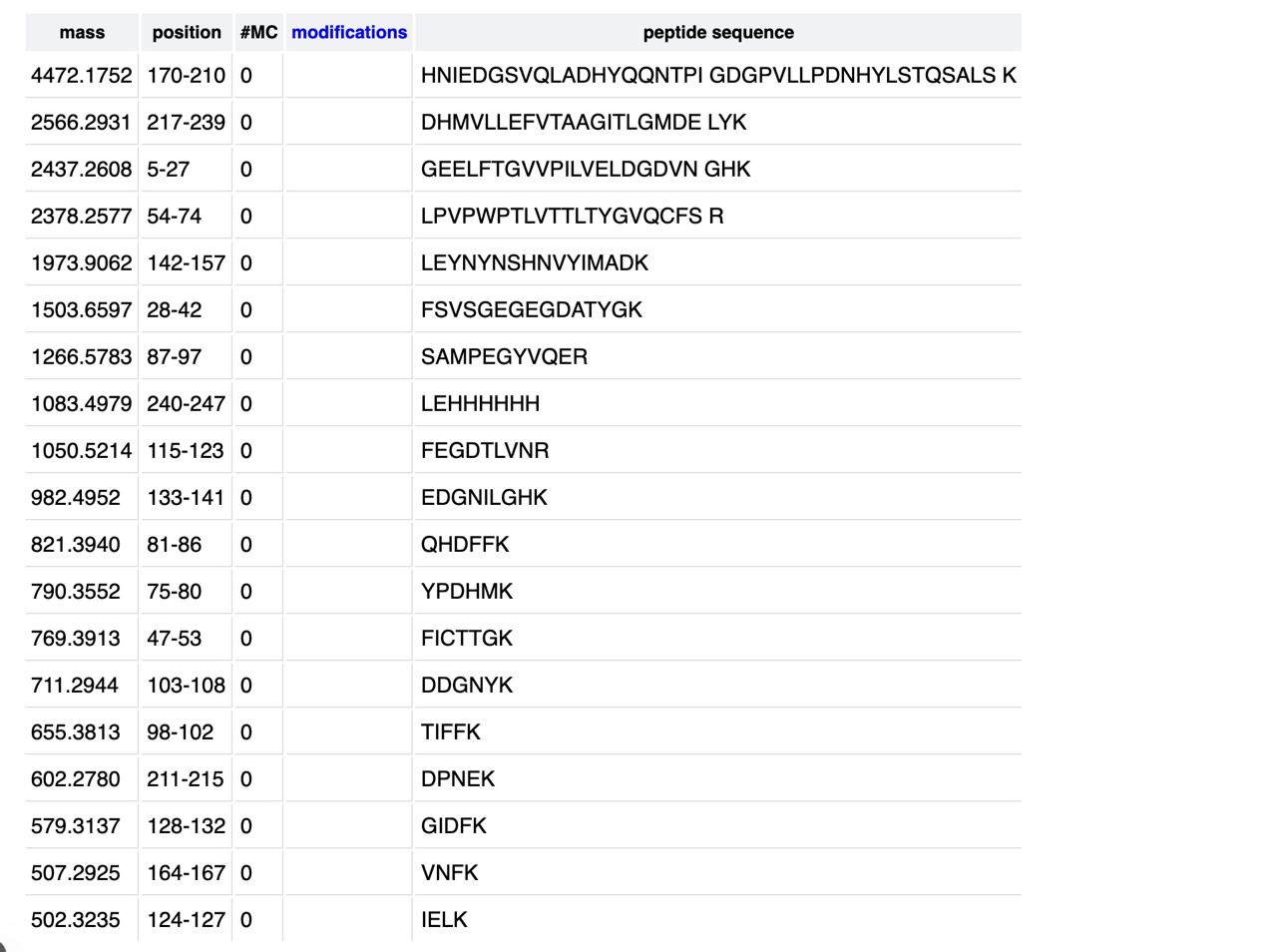
Calculate Expected Masses for Each Species
Using the polypeptide subunit masses from Table 1:
the expected masses are:
| Oligomeric Species | Subunit Mass | # Subunits | Calculated Mass (polypeptide only) |
|---|---|---|---|
| 7FU Decamer | 340 kDa | 10 | 3,400 kDa = 3.4 MDa |
| 8FU Didecamer | 400 kDa | 20 | 8,000 kDa = 8.0 MDa |
| 8FU 3-Decamer | 400 kDa | 30 | 12,000 kDa = 12.0 MDa |
| 8FU 4-Decamer | 400 kDa | 40 | 16,000 kDa = 16.0 MDa |
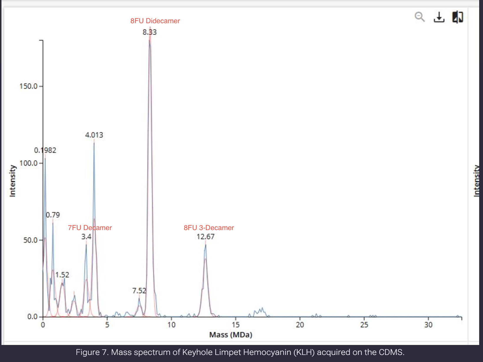
N/A
I missed the opportunity to contribute to the HTGAA CFPS bioart project. Later, I contributed to the SynBioBeta bioart project. I worked on part of the DNA on the center-left plate.
What I liked: This kind of community-coordinated experiment builds genuine shared investment in the outcome, which is a rare and valuable pedagogical achievement.
What could be improved: For future years, giving participants a low-resolution preview of the emerging canvas in near-real-time — without revealing the final image — would heighten the sense of collective emergence and encourage more strategic pixel placement.
1. Referencing the cell-free protein synthesis reaction composition E. coli Lysate
BL21 (DE3) Star Lysate (includes T7 RNA Polymerase): The crude cell lysate supplies the entire transcription-translation (TX-TL) machinery — ribosomes, tRNA synthetases, elongation and initiation factors, chaperones, and co-factors — needed to convert DNA template into protein in vitro; the BL21 DE3 strain is specifically engineered to co-express T7 RNA Polymerase (from the chromosomal DE3 insertion), which is essential for driving transcription from the T7φ10 promoter used on most CFPS expression plasmids.
Salts/Buffer
Potassium Glutamate: The primary intracellular-mimicking monovalent cation that stabilises ribosome conformation and partially replaces KCl to avoid chloride-induced inhibition; potassium ions are critical for maintaining ribosome association and translational fidelity.
HEPES-KOH pH 7.5: A zwitterionic biological buffer that maintains reaction pH close to physiological values throughout the synthesis reaction, preventing the accumulation of protons that would otherwise inactivate ribosomes and enzymes as phosphate is metabolised.
Magnesium Glutamate: Provides free Mg²⁺ ions, which are indispensable cofactors for ribosome assembly, RNA polymerase activity, and the enzymatic reactions of the energy regeneration system; Mg²⁺ concentration is one of the most sensitive optimisation parameters in CFPS and must be carefully titrated for each lysate batch.
Potassium Phosphate Monobasic / Dibasic: Phosphate ions participate in energy metabolism and buffer secondary pH fluctuations; they also serve as inorganic phosphate donors and are required for metabolic pathways within the lysate.
Energy / Nucleotide System
Ribose: A five-carbon sugar that serves as the backbone of nucleoside synthesis; in the NMP-Ribose-Glucose system, ribose provides the sugar moiety for regenerating nucleoside monophosphates through the pentose phosphate pathway and purine/pyrimidine salvage enzymes present in the lysate.
Glucose: The primary carbon and energy source for ATP regeneration via glycolysis; endogenous glycolytic enzymes in the lysate convert glucose to pyruvate, generating ATP and NADH needed to sustain transcription and translation over extended reaction times.
AMP, CMP, GMP, UMP: Nucleoside monophosphates (NMPs) that serve as precursors for NTP synthesis; rather than supplementing expensive pre-formed NTPs, the NMP-based system relies on endogenous nucleoside monophosphate kinases (NMPK) and pyruvate kinase within the lysate to phosphorylate these precursors to the triphosphate form needed for transcription.
Guanine: A free purine base that feeds the guanosine salvage pathway; nucleoside phosphorylase enzymes in the lysate convert guanine + ribose-1-phosphate to guanosine, which is then phosphorylated to GMP and ultimately GTP — providing an additional low-cost input for GTP pools without supplying GMP directly.
Translation Mix (Amino Acids)
17 Amino Acid Mix: Provides the bulk of the 20 canonical amino acids needed for polypeptide elongation; splitting the amino acid supply allows independent supplementation of the three most problematic residues that tend to degrade, oxidise, or precipitate under standard CFPS conditions.
Tyrosine: Supplied separately because tyrosine has very low aqueous solubility at neutral pH and precipitates out of a premixed solution; it is added as a separately prepared suspension or at low concentration to ensure it remains bioavailable during the reaction.
Cysteine: Added separately because cysteine is prone to oxidative degradation — it dimerises to cystine under aerobic conditions — so it is freshly prepared and added just before the reaction to maintain a sufficient pool for proteins requiring cysteine residues.
Additives
Nicotinamide: A precursor to NAD⁺, which is an essential redox cofactor for glycolysis (particularly the GAPDH reaction); supplementing nicotinamide ensures the lysate can regenerate NAD⁺ from NADH during glucose catabolism, sustaining the energy regeneration capacity of the reaction over long incubations.
Backfill
Nuclease Free Water: Added to bring the reaction to the desired final volume without introducing RNases or DNases that would degrade the RNA polymerase transcript or the DNA template; using nuclease-free water is essential to protect the mRNA intermediates produced during transcription.
2. Describe the main differences between the 1-hour optimized PEP-NTP master mix and the 20-hour NMP-Ribose-Glucose master mix The 1-hour PEP–NTP system uses phosphoenolpyruvate (PEP) as a high-energy phosphate donor to rapidly regenerate ATP via pyruvate kinase and relies on pre-formed NTPs, producing a short, intense burst of energy that supports fast, high-yield protein synthesis before quickly terminating as PEP is depleted. In contrast, the 20-hour NMP–Ribose–Glucose system uses glucose-driven metabolism for continuous ATP regeneration and enzymatic phosphorylation of NMPs into NTPs, enabling slower but long-duration protein expression at lower cost and is preferred for sustained experiments.
1. Given the 6 fluorescent proteins we used for our collaborative painting, identify and explain at least one biophysical or functional property of each protein that affects expression or readout in cell-free systems.
i. sfGFP (superfolder GFP)
sfGFP is engineered for very fast, robust β‑barrel folding, giving near-complete folding efficiency even when fused to aggregation-prone partners and making it a reliable baseline reporter for CFPS optimization. Its chromophore maturation requires molecular oxygen, so oxygen availability will affect fluorescence in cell-free reactions.
ii. mRFP1
mRFP1 has relatively slow chromophore maturation, meaning early-time fluorescence can substantially underreport total protein synthesis if fluorescence alone is used as a proxy. Its chromophore formation depends on molecular oxygen.
iii. mKO2
mKO2 is a fast-folding orange FP but retains acid sensitivity, so its fluorescence can be quenched if the cell-free reaction drifts acidic during prolonged incubations. This pH vulnerability should be monitored in long or metabolically active CFPS systems.
iv. mTurquoise2
mTurquoise2 is an intrinsically bright cyan FP with very high quantum yield, but native cysteines can form disulfide-linked oligomers in oxidising conditions, reducing the fraction of fluorescent protein. In cell-free systems, including reducing agents may be necessary, and its slower maturation versus sfGFP affects early readouts.
v. mScarlet-I
mScarlet-I is a bright, monomeric red FP with fast maturation and good photostability, making it a robust red reporter for long cell-free incubations and oxidising conditions. Its high intrinsic brightness supports sensitive fluorometric detection.
vi. Electra2
Electra2 is a relatively bright blue FP but blue FPs typically produce lower absolute signal than green or red FPs under equivalent expression, so overall fluorescence will be lower. It has reported tendencies to aggregate in some contexts, which can reduce soluble, fluorescent yield in CFPS.
2. Create a hypothesis for how adjusting one or more reagents in the cell-free mastermix could improve a specific biophysical or functional property you identified above, in order to maximize fluorescence over a 36-hour incubation. Clearly state the protein, the reagent(s), and the expected effect.
Protein targeted: mKO2
Property identified: Acid sensitivity — mKO2 fluorescence is quenched at lower pH, and the NMP-Ribose-Glucose system can accumulate acidic byproducts over a 36‑hour incubation that may shift reaction pH downward.
Hypothesis: Increasing buffer capacity (HEPES-KOH from ~50 mM to ~100–150 mM and/or adding elevated potassium phosphate dibasic) will maintain pH ~7.2–7.8 and preserve mKO2 chromophore protonation; alternatively, reducing glucose to ~50% could slow acid production at the cost of some ATP regeneration.
Expected effect: Higher buffer capacity and/or reduced glucose should yield increased mKO2 fluorescence at 20–36 h versus standard mix, with a possible reduction in early (0–6 h) peak expression; test by plotting fluorescence kinetics across buffer and glucose gradients.

Framework: Learn → Design → Build → Test (Clark-ElSayed et al., 2025)
Chloroplast cell-free expression (CFE) systems have recently been established as powerful rapid-prototyping platforms for plastid genetic parts, yet whether these systems can support synthetic RNA logic remains entirely untested. Toehold switches — de novo-designed riboregulators that activate translation in response to specific trigger RNAs — represent the most sophisticated programmable RNA gates in synthetic biology. Machine learning models trained on E. coli CFE data have begun to extract sequence-structure features predictive of switch performance using frameworks like SANDSTORM (Riley et al., 2025), but whether those learned relationships hold in a chloroplast ribosome context is unknown. This project addresses that gap directly by applying the Learn-Design-Build-Test (LDBT) framework to map the thermodynamic rules governing toehold switch function in spinach chloroplast CFE.
We train a SANDSTORM predictive neural network — a dual-input CNN incorporating one-hot-encoded RNA sequence and secondary structure arrays (Riley et al., 2025) — on the publicly available 181-switch E. coli dataset to learn sequence-structure-function relationships for toehold switches. The trained SANDSTORM model is then paired with GARDN (Generative Adversarial RNA Design Network) to generate 12–15 novel toehold switch candidates with predicted high ON/OFF performance in a chloroplast ribosome context, including PVY coat protein mRNA-triggered designs. Whole plasmid constructs are ordered from Twist Bioscience and tested in both spinach chloroplast CFE and crude E. coli S30 extract; a secondary SANDSTORM model retrained on the resulting chloroplast data constitutes the first sequence-structure-function ML model for toehold switches in a plant-native ribosomal context.
The project produces the first empirical dataset and neural network model for toehold switch performance in plant chloroplast CFE, a transferable GARDN-SANDSTORM LDBT workflow applicable to any novel ribosome context, and a foundation for programmable RNA diagnostics manufacturable directly from plant material. All experiments are performed using the Ginkgo Bioworks autonomous laboratory infrastructure and open-access grocery-store spinach, demonstrating that LDBT with deep learning is executable at global-access scale with a materials budget under $1,200.
Decode the sequence-structure rules governing translation initiation in the chloroplast ribosomal context by quantifying ON/OFF ratios for 12–15 GARDN-SANDSTORM-designed toehold switch candidates in spinach chloroplast CFE via Ginkgo Bioworks automation and NanoLuc readout, then retraining SANDSTORM on the resulting dataset to encode the sequence-structure-function relationships that define programmable RNA regulation in the plastid ribosomal context.
The LDBT workflow proceeds as follows:
The retrained L2 model and its integrated gradients attribution maps — not solely the ON/OFF numbers — constitute the primary scientific deliverable.
Scale to 100+ toehold switch constructs across spinach, wheat, and poplar to train a converged, chloroplast-specific SANDSTORM model above its 384-sequence reliability threshold (Riley et al., 2025), then extend GARDN generative design toward multi-input RNA logic gates — AND gates, cascades, and riboregulator networks — establishing the first generative design grammar for programmable RNA circuits in plant plastids. Concurrent optimization of the automated CFE workflow at Ginkgo Bioworks will enable 384-well throughput across species, and the resulting pan-plant SANDSTORM model, GARDN design weights, and logic gate characterization data will be deposited to Zenodo as a community resource, marking a transition from individual switch quantification to a systematic engineering discipline for chloroplast RNA circuits.
Leverage the chloroplast RNA circuit design grammar to open two parallel application frontiers: inducible biomanufacturing in plastids — conditional recombinant protein expression triggered by endogenous RNA signals, bypassing the constitutive expression ceiling of current plastid systems — and equipment-free crop pathogen biosensors using lyophilized chloroplast CFE reactions that detect Potato Virus Y, cassava mosaic virus, and wheat blast RNA signatures in the field without cold chain or laboratory infrastructure. Together, these applications reframe plant material not as passive agricultural output but as a substrate for programmable molecular manufacturing, and position the GARDN-SANDSTORM chloroplast platform as the foundation for plastid synthetic biology as a mature, generalizable engineering discipline.
Bohm et al. | Clark et al. |
LDBT | Alexander A. Green et al. |
Aidan T. Riley et al. |
Green et al. (2014) established toehold switches as programmable RNA regulators achieving >400-fold ON/OFF dynamic range in E. coli, with sequence-programmable targeting to any trigger RNA (Cell, 167, 246–259). Their 168-switch dataset defines the architectural constraints reproduced in all Twist Bioscience constructs here and constitutes the primary SANDSTORM training set.
Riley et al. (2025) introduced SANDSTORM and GARDN as a paired predictive-generative framework: SANDSTORM encodes RNA as dual one-hot sequence and secondary structure inputs, achieves accurate predictions from as few as 384 training examples, and outperforms classical thermodynamic algorithms; GARDN generates novel candidates with targeted experimental attributes (Nature Communications). The current project trains SANDSTORM on Green et al.’s E. coli dataset, uses GARDN to generate 12–15 chloroplast-targeted toehold switch candidates, and retrains SANDSTORM on the resulting chloroplast CFE data.
Clark, Voigt & Jewett (2024) established the first high-yield tobacco chloroplast CFE system, achieving 60 ± 4 μg/mL NanoLuc yields and a 1,300-fold expression dynamic range across 103 RBS variants screened in under one day (ACS Synthetic Biology). Böhm, Inckemann et al. (2024) extended this platform to spinach, wheat, and poplar using nanolitre-scale automation, demonstrating a >4-log dynamic range and R² = 0.93 cross-species expression correlation between spinach and wheat — motivating spinach as the training organism and wheat as the generalisation target (ACS Synthetic Biology). Clark-ElSayed et al. (2025) formalised the LDBT paradigm, positioning ML at the start of the engineering cycle and CFE as the high-throughput data-generation engine (Nature Communications); this project instantiates that paradigm exactly.
Knowledge gap: No study has measured toehold switch ON/OFF ratios in plant chloroplast CFE, applied SANDSTORM or GARDN to a chloroplast ribosome context, or retrained either model on chloroplast expression data. The chloroplast ribosome is evolutionarily prokaryotic but operates at 20–25°C with a distinct anti-Shine-Dalgarno sequence and ionic environment, making transfer of E. coli-learned sequence-structure-function relationships non-obvious and experimentally unvalidated.
This project is novel in three respects that together constitute an unstudied intersection of existing capabilities:
Chloroplast cell-free expression is emerging as a transformative rapid-prototyping platform for plant synthetic biology, yet it currently lacks the programmable regulatory logic — inducible switches, conditional circuits, RNA-responsive gates — that makes E. coli CFE a mature engineering substrate. This project addresses that foundational gap: by establishing the first sequence-structure-function dataset and neural network model for toehold switch performance in a plant organellar ribosome context, it provides the missing design layer that allows chloroplast CFE to move from constitutive expression screening toward programmable, input-responsive genetic circuits.
The GARDN-SANDSTORM LDBT workflow is not a single-use tool but a reusable design engine — analogous to the role the Salis RBS Calculator played in standardising translational control in E. coli — and the Zenodo-deposited dataset and model weights constitute community infrastructure any laboratory can build upon. Each experimental round expands the L2 model, progressively improving predictive accuracy and enabling generative design of increasingly complex RNA circuits without proportional increases in experimental cost.
At the application frontier, this infrastructure enables inducible biomanufacturing in plastids (Aim 2) and field-deployable lyophilised biosensors for crop pathogens including Potato Virus Y — which causes billions of dollars in annual losses globally — requiring no cold chain, no laboratory infrastructure, and no purified proteins (Aim 3). Demonstrating the full LDBT cycle at student-project scale with grocery-store spinach and a sub-$1,200 budget establishes a precedent for globally accessible synthetic biology development that does not require centralised biofoundry resources.
Ethical Implications: This project operates at the intersection of biosensing technology and agricultural systems, which raises considerations spanning the principles of beneficence, justice, and responsibility. The beneficence argument is strong: a low-cost, field-deployable diagnostic for crop pathogens could protect food security for smallholder farmers who currently have no access to pathogen surveillance. However, the justice dimension requires scrutiny — specifically, who controls the technology if it is developed from an open-source student project, who benefits from its commercialization, and whether the communities most affected by PVY losses have meaningful voice in how the tool is designed and deployed. The dual-use dimension is minimal but non-trivially zero: a toehold switch system designed to detect a plant pathogen RNA could, in principle, be reprogrammed to detect other RNA sequences; the framework is sequence-agnostic. The principle of non-maleficence requires acknowledging that a field biosensor producing false-negatives could provide false assurance, while false-positives could trigger unnecessary crop destruction. The current project makes no diagnostic claims — it tests the enabling molecular component — but responsible downstream development must address sensitivity and specificity thresholds before any field deployment claim.
Responsible Implementation: The measures taken in this project to ensure ethical research practice include:
Potential unintended consequences of the broader vision — field-deployed toehold switch biosensors — include misuse for detecting human pathogens without regulatory oversight, and the displacement of existing laboratory diagnostic workers if the technology is deployed without appropriate workforce transition planning. Alternatives to the toehold switch approach, including CRISPR-Cas13-based diagnostics (SHERLOCK) and lateral flow immunoassays, should be evaluated comparatively in any future regulatory submission, and the assumptions of sequence-structure-function transferability across ribosome contexts validated in additional plant species before field deployment claims are made.
Timeline Overview: Dry-lab phases (L1, D) run in parallel with extract preparation (B); total wet lab execution is 5 weeks at Ginkgo Bioworks node.
| Field | Detail |
|---|---|
| Purpose | Prepare dual-channel SANDSTORM input tensors from the 181-switch E. coli dataset |
| Method | Download the 181-switch ON/OFF dataset (Green et al. 2014 + 2017, as compiled by To et al. 2018). For each sequence, compute the N×N structural array: position (i,j) = 0 if no canonical pairing possible; 2 if A-U or G-U wobble; 3 if G-C. Values encode hydrogen bond capacity from nucleotide identity alone — no folding software, no temperature assumption. Pair with one-hot-encoded sequences as dual-channel SANDSTORM input. Load pretrained SANDSTORM weights from the Angenent-Mari et al. (2020) toehold dataset via the GARDN-SANDSTORM repository for transfer learning initialisation. |
| Automation | Dry lab (Python/Jupyter); no Ginkgo machine required |
| Plate | N/A |
| Expected result | 181 paired input tensors computed in < 1 min; pretrained weights loaded; fine-tuning pipeline confirmed |
| Timeline | Days 1–2 |
| Field | Detail |
|---|---|
| Purpose | Fine-tune SANDSTORM on the 181-switch E. coli dataset to learn sequence-structure-function relationships |
| Method | Fine-tune pretrained SANDSTORM (two parallel CNN stacks: one for one-hot sequence with batch normalisation between layers 1–2; one for structural array with spatial dropout 0.2 and GlobalMaxPooling2D; concatenated outputs through three dense layers; ReLU activations; Adam optimiser). 80/20 training-testing split stratified by ON/OFF ratio, averaged across three randomised splits. Report Spearman r, R², MSE. Benchmark against NuSpeak/STORM. Rank all 181 switches by predicted ON/OFF. |
| Automation | Dry lab |
| Plate | N/A |
| Expected result | Spearman r ≥ 0.4 after fine-tuning; ranked switch list available for GARDN design guidance |
| Timeline | Day 2 |
| Field | Detail |
|---|---|
| Purpose | Generate 12–15 novel toehold switch sequences optimised for high predicted ON/OFF performance |
| Method | GARDN generator (WGAN-GP; upsampling layers (2,5),(2,6),(1,2); spectrally normalised conv layers; batch normalisation) produces 60-nt switch sequences from latent variable Z. Programmable reverse-complementation layer enforces canonical stem-loop grammar by construction. Frozen SANDSTORM L1 predictor guides optimisation by gradient ascent: Z → Z + α∇_Z P_δ(G_θ(Z)), 300 steps, structural array recomputed from sequence at each step (O(N²), no folding calls). Generate 300 candidates; select 9–12 highest predicted ON/OFF. For ≥ 3 PVY-triggered designs, specify trigger from DQ157180 coat protein ORF (nt 8,950–9,200) to constrain the reverse-complementation layer. Verify trigger self-folding: NUPACK ΔG_MFE > −3 kcal/mol at 25°C. Include one scrambled-trigger negative control and one unstructured RBS positive control. |
| Automation | Dry lab; NUPACK for trigger verification only |
| Plate | N/A |
| Expected result | 12–15 GARDN-SANDSTORM-designed sequences; structural agreement score ~0.92; ≥ 3 PVY-targeted; optimisation runtime ~11 s per 300 calls |
| Timeline | Days 2–4 |
| Field | Detail |
|---|---|
| Purpose | Order all 12–15 constructs as sequence-verified whole plasmids from Twist Bioscience |
| Method | Design each construct as a complete circular plasmid: T7 promoter → toehold switch module (12-nt toehold + 18-nt stem + 11-nt loop + 18-nt stem complement) → Shine-Dalgarno RBS linker → ATG → NanoLuc ORF (513 bp) → T7 terminator → pUC19 backbone (AmpR, pMB1 ori). Total plasmid size ~3,250 bp. Prepare GenBank files in Benchling. Screen all sequences through SecureDNA before submission. Submit to Twist Bioscience Clonal Gene service (pUC19 backbone). |
| Automation | Benchling (design); Twist portal (order); SecureDNA (screening) |
| Plate | N/A |
| Expected result | 12–15 whole plasmid constructs delivered lyophilised within 7–10 business days |
| Timeline | Days 3–5 |
Representative GenBank construct — TS-PVY-01:
The following GenBank file encodes the first PVY-targeted toehold switch, ordered as a whole plasmid from Twist Bioscience. Trigger sequence is derived from PVY coat protein mRNA (DQ157180, ~nt 8,960–8,989). Paste directly into the Twist upload portal and select the pUC19 clonal backbone.
A total of 12–15 analogous GenBank files are prepared in Benchling, each with unique toehold/stem sequences. All are ordered as whole plasmids from Twist Bioscience. The backbone (pUC19, AmpR, pMB1 ori) is identical across all constructs.
| Field | Detail |
|---|---|
| Purpose | Produce PVY trigger RNAs and Green et al. subset trigger RNAs for CFE assays |
| Method | PCR-amplify T7 promoter-tagged templates from IDT gBlocks encoding the DQ157180 coat protein target region using ATC Thermal Cycler. In vitro transcribe using NEB HiScribe T7 High Yield RNA Synthesis Kit. Purify by lithium chloride precipitation. Quantify by Nanodrop (A260). Verify integrity by Agilent TapeStation. Order Green et al. subset trigger RNAs (5 sequences) as HPLC-purified RNA oligonucleotides from IDT. |
| Automation | ATC Thermal Cycler (PCR); manual IVT and purification |
| Plate | 96-Armadillo-PCR-AB2396X (PCR step) |
| Expected result | PVY trigger RNA ≥ 1 μg/μL; A260/A280 > 1.9; intact band on TapeStation |
| Timeline | Week 2, Days 3–5 |
| Field | Detail |
|---|---|
| Purpose | Prepare active spinach chloroplast extract for CFE reactions |
| Method | Homogenise two independent 100 g batches of grocery-store spinach in 200 mL ice-cold Extraction Buffer (50 mM HEPES-KOH pH 8.0 / 2 mM EDTA / 330 mM sorbitol / 0.6% w/v PVP-40 / 0.1% BSA / 5 mM β-mercaptoethanol) for 30 s in a pre-chilled blender. Filter through two layers of Miracloth. Centrifuge at 1,000×g, 8 min, 4°C (retain green pellet). Wash pellet twice in Extraction Buffer (1,000×g, 8 min). Resuspend in Lysis Buffer (30 mM HEPES-KOH pH 7.7 / 60 mM KOAc / 7 mM MgOAc / 60 mM NH₄OAc / 10% glycerol / 5 mM DTT / 0.5 mM PMSF). Lyse by 15–20 passes through a 25G × 40 mm syringe needle. Primary clarification: centrifuge at 30,000×g, 30 min, 4°C (twice) if ultracentrifuge available. Contingency fallback: if 30,000×g is unavailable, perform an additional 5-min 1,000×g pre-spin, then clarify at 16,000×g for 30 min, 4°C (twice); note this may reduce extract clarity and yield by up to 30% and should be documented as a protocol deviation. Dialyse supernatant in Slide-A-Lyzer 10K MWCO cassettes against 200 mL Lysis Buffer for 2 × 2 h at 4°C. Final centrifuge at 30,000×g (or 16,000×g fallback), 20 min, 4°C. Aliquot 20 μL; snap-freeze in liquid nitrogen; store at −80°C. |
| Automation | HiG Centrifuge (1,000×g steps); manual syringe lysis; Cytomat (−80°C storage) |
| Plate | N/A (bulk extract preparation) |
| Expected result | Two independent 20 μL aliquot sets; active extract with green tint (residual chlorophyll) |
| Timeline | Week 3, Days 1–3 |
| Field | Detail |
|---|---|
| Purpose | Confirm translational activity of both extract batches before proceeding to switch assays |
| Method | Test both batches using Addgene #216625 (Böhm et al. universal test construct). Prepare reactions in 384-well Greiner black clear-bottom plates. Dispense master mix via Tempest bulk dispenser; add DNA template via Echo525; seal with Plateloc (A4s breathable seal); incubate at 25°C in Inheco Plate Incubator. Measure NanoLuc luminescence at t = 2 h and t = 4 h on PHERAstar FSX (LUM module, 460 nm emission). If signal < 5-fold above buffer-only blank: troubleshoot (verify glycerol, PVP, dialysis, centrifuge speed) before proceeding. |
| Automation | Tempest (master mix); Echo525 (DNA); Plateloc + A4s (sealing); Inheco (incubation); PHERAstar FSX (detection) |
| Plate | 384 Greiner black-well clear-bottom |
| Expected result | ≥ 5-fold signal above blank at t = 4 h; batch-to-batch agreement within 2-fold |
| Timeline | Week 3, Day 3 |
| Field | Detail |
|---|---|
| Purpose | Identify the optimal kinetic endpoint and trigger RNA concentration for all subsequent assays |
| Method | Measure NanoLuc for the positive control construct at t = 1, 2, 3, 4, 5, 6, 8, and 12 h (PHERAstar FSX, 384-well Greiner black clear-bottom). Identify plateau time point (< 10% increase between consecutive measurements). Separately, test one high-predicted-performance switch at trigger concentrations of 0.01, 0.1, 1, 5, and 10 nM (switch template fixed at 2 nM). Measure ON/OFF ratio at the kinetically validated endpoint. Use the concentration maximising ON/OFF ratio uniformly across all switches. |
| Automation | Echo525 (trigger dilutions); Inheco (incubation); PHERAstar FSX (detection) |
| Plate | 384 Greiner black-well clear-bottom |
| Expected result | Plateau at ~3–5 h; optimal trigger concentration 0.1–1 nM |
| Timeline | Week 3, Days 4–5 |
| Field | Detail |
|---|---|
| Purpose | Measure NanoLuc ON/OFF ratios for all 12–15 toehold switch candidates in spinach chloroplast CFE |
| Method | Full automated workflow (see table below). Each switch run in four conditions × ≥ 3 technical replicates. ON/OFF ratio formula: (Condition B − D) / (Condition A − D). |
| Automation | Tempest → Echo525 → Plateloc + A4s → Inheco → XPeel → PHERAstar FSX |
| Plate | 384 Greiner black-well clear-bottom (reactions); 384-well Echo PP (source plate) |
| Expected result | Measurable NanoLuc signal across all ON-state conditions; ON/OFF ratios spanning ≥ 2-fold dynamic range across 12–15 switches |
| Timeline | Weeks 4–5 |
Automated Workflow Table:
| Sub-step | Machine | Plate Type | Action |
|---|---|---|---|
| Master mix dispensing | Tempest | 384 Greiner black clear-bottom | Dispense CFE master mix (buffer + NTPs + amino acids) to all wells |
| DNA template addition | Echo525 | 384-well Echo PP (source) | Acoustic transfer of whole plasmid DNA (1–2 nM final) |
| Trigger RNA addition | Echo525 | 384-well Echo PP (source) | Acoustic transfer of trigger RNAs at pilot-optimised concentration |
| Plate sealing | Plateloc + A4s | — | Breathable seal to prevent evaporation while allowing gas exchange |
| CFE incubation | Inheco Plate Incubator | 384 Greiner black clear-bottom | 25°C for plateau endpoint duration |
| Seal removal | XPeel | — | Remove breathable seal before detection |
| Luminescence readout | PHERAstar FSX | 384 Greiner black clear-bottom | NanoLuc luminescence (LUM module, 460 nm emission) |
| Data export | — | — | Export raw RLU values; compute ON/OFF ratios |
384-Well Plate Assay Layout (1 plate = 3 switches × 4 conditions × 4 replicates + controls):
Legend:
OFF = Switch construct, no trigger (OFF-state leakage)ON = Switch construct + cognate trigger at pilot-optimised concentrationSPE = Switch construct + scrambled non-cognate trigger (specificity control)BLK = No template, no trigger (background)POS = Unstructured RBS construct (maximum ON-state reference)ON/OFF ratio = (Condition ON − BLK) / (Condition OFF − BLK)
| Field | Detail |
|---|---|
| Purpose | Train the first sequence-structure-function ML model for toehold switches in a plant organellar ribosome context |
| Method | Compute structural arrays for all 12–15 GARDN-designed switches using the same purely sequence-based method as Step 1 (N×N Watson-Crick possibility matrix; values 0/2/3 from nucleotide identities alone; no folding software). Retrain SANDSTORM on measured chloroplast CFE ON/OFF data (n = 12–15) using leave-one-out cross-validation (LOOCV), initialising with L1 E. coli model weights (transfer learning). Apply integrated gradients to the structural input channel to reveal which sequence positions and pairing interactions most strongly drive chloroplast ON/OFF predictions. |
| Automation | Dry lab |
| Plate | N/A |
| Expected result | SANDSTORM L2 converges; LOOCV Spearman r ± SD reported; integrated gradients attribution maps generated for structural channel |
| Timeline | Week 5, Day 1 |
| Field | Detail |
|---|---|
| Purpose | Identify which structural positions shift in importance between E. coli and chloroplast ribosome contexts |
| Method | Compare LOOCV Spearman r ± SD between L1 and L2 models. Apply integrated gradients to both models’ structural input channels for a canonical toehold switch. Compare attribution maps to identify positions where the model weights pairing interactions differently in the chloroplast vs. E. coli context. Positions corresponding to stem stability and RBS accessibility are expected to show the largest attribution shifts. |
| Automation | Dry lab |
| Plate | N/A |
| Expected result | Attribution maps differ between L1 and L2; LOOCV Spearman r > 0.2 in L2 indicates sequence-structure features are informative even at n = 12–15 with transfer learning initialisation |
| Timeline | Week 5, Day 2 |
| Field | Detail |
|---|---|
| Purpose | Determine whether sequence-structure-function patterns learned from E. coli data predict chloroplast CFE performance |
| Method | Compute Spearman r between L1 SANDSTORM predicted ON/OFF rankings and measured chloroplast CFE ON/OFF ratios. The same structural arrays computed in Step 1 are used — the structural array is sequence-derived and temperature-independent. If Spearman r > 0.4: patterns generalise across ribosome contexts. If r ≈ 0: the chloroplast context requires its own training data, making the L2 dataset the necessary foundation. Compare integrated gradient attribution maps between L1 and L2 to identify which structural positions shift in importance. |
| Automation | Dry lab |
| Plate | N/A |
| Expected result | Partial transfer (Spearman r ≈ 0.3–0.5); L2 attribution maps diverge from L1 at stem-stability and RBS-exposure positions |
| Timeline | Week 5, Day 2 |
| Field | Detail |
|---|---|
| Purpose | Quantify how faithfully each GARDN-designed switch adheres to canonical toehold switch geometry and correlate with measured ON/OFF ratios |
| Method | For each of the 12–15 switches, predict MFE secondary structure in dot-bracket notation using NUPACK (the only step in the project where NUPACK is used — for post-hoc MFE structure visualisation, not for SANDSTORM input arrays). Compute structural agreement score: (1/N) Σ p(i), where p(i) is the probability of position i adopting the dot-bracket symbol matching the canonical target structure …………(((((((((…((((((………..))))))…)))))))))). Plot structural agreement score against measured chloroplast ON/OFF ratio and against measured E. coli ON/OFF ratio. |
| Automation | Dry lab |
| Plate | N/A |
| Expected result | Structural agreement scores cluster near ~0.92 (Riley et al. Fig. 5h); switches below 0.80 flagged as likely low-performance outliers |
| Timeline | Week 5, Days 3–4 |
| Field | Detail |
|---|---|
| Purpose | Assess extract batch-to-batch reproducibility and determine whether data from both batches can be pooled for ML training |
| Method | For three cross-batch reference switches (one high / medium / low predicted performance), compare ON/OFF ratios between the two independent extract batches. If batch-to-batch CV < 30%: include all data in ML training. If CV > 30%: restrict to higher-quality batch and note as limitation. |
| Automation | Data analysis (dry lab) |
| Plate | N/A |
| Expected result | CV < 30% for high-performance switches; possibly higher CV for low-performance switches near the detection limit |
| Timeline | Week 5, Day 5 |
| Field | Detail |
|---|---|
| Purpose | Make all data, model weights, and analysis publicly available; prepare final figures for presentation |
| Method | Deposit all raw luminescence values, computed ON/OFF ratios, GARDN-SANDSTORM model weights (L1 and L2), structural arrays, and trained model outputs to Zenodo (DOI minted before May 13 presentation), mirrored to GitHub following the GARDN-SANDSTORM repository structure. Prepare final figures: (1) ON/OFF ratio bar chart for all 12–15 switches across both systems; (2) scatter plot of SANDSTORM L1 predicted vs. chloroplast measured ON/OFF (transfer learning test); (3) integrated gradient attribution map comparison between L1 and L2 structural channels; (4) structural agreement scores for all GARDN-designed candidates vs. Riley et al. experimental dataset reference. |
| Automation | Dry lab |
| Plate | N/A |
| Expected result | Complete open dataset and model weights available to the community; full LDBT cycle with GARDN-SANDSTORM documented as a reproducible workflow |
| Timeline | Week 6 |
| Technique | Relevant? |
|---|---|
| Pipetting | ✅ |
| Lab Safety | ✅ |
| Bioethical Considerations | ✅ (required) |
| DNA Construct Design | ✅ |
| Databases (GenBank, NCBI, Ensembl) | ✅ |
| DNA Sequencing | ❌ (Twist provides sequence-verified plasmids) |
| Restriction Enzyme Digestion | ❌ (whole plasmid from Twist; no cloning) |
| Gel Electrophoresis | ❌ (not in primary workflow) |
| Creating Code for Laboratory Automation | ✅ |
| Designing a Twist Order | ✅ |
| Creating a plan to use the Autonomous Lab at Ginkgo Bioworks | ✅ |
| Bacterial Culturing | ✅ (E. coli BL21(DE3) for S30 extract) |
| Bacterial Processing (Centrifugation, Lysis, Purification) | ✅ |
| Cell-Free Reactions | ✅ |
| Freeze-Dried Cell-Free Systems | ❌ (not in Aim 1; potential Aim 3 application) |
| PCR Reactions | ✅ (IVT template generation, Step 5) |
| Gibson Assembly | ❌ (not required; whole plasmid from Twist) |
| Use of Benchling | ✅ |
| Models and Notebooks | ✅ (SANDSTORM CNN + GARDN) |
| Databases | ✅ (Green et al. dataset; GenBank NC_002202.1; To et al. 2018) |
| CRISPR/Cas9 | ❌ |
Technique 1: Cell-Free Reactions
Cell-free expression (CFE) systems are in vitro transcription-translation platforms derived from cellular lysates that retain the molecular machinery for gene expression without intact living cells. In this project, CFE is the core experimental platform: spinach chloroplast extract is prepared from commercial grocery-store spinach and supplemented with a master mix containing NTPs, amino acids, and energy regeneration components, enabling NanoLuc luciferase production from the toehold switch plasmid templates ordered from Twist Bioscience. The use of CFE is scientifically essential rather than merely convenient — it allows direct measurement of toehold switch function in a chloroplast ribosome context without the confound of chloroplast transformation, which would require months of plant growth and selection. Additionally, the open nature of the CFE system permits precise control of trigger RNA concentration, template DNA concentration, and reaction composition in a way impossible in intact plastids, making CFE the ideal platform for the quantitative sequence-structure-function analysis via GARDN-SANDSTORM that is central to the LDBT workflow.
Technique 2: GARDN-SANDSTORM Generative RNA Design (Models and Notebooks)
GARDN-SANDSTORM is a paired generative-predictive deep learning framework developed by Riley et al. (2025, Nature Communications) specifically for functional RNA design, consisting of two components: SANDSTORM (a dual-input CNN accepting one-hot-encoded RNA sequence alongside a purely sequence-derived N×N structural array encoding Watson-Crick base-pairing possibilities to predict function) and GARDN (a Wasserstein GAN with gradient penalty incorporating a programmable reverse-complementation output layer that enforces the canonical toehold switch stem-loop grammar during generation by construction, rather than requiring post-hoc correction). The key innovation of the structural array is its temperature-independence and computational efficiency: because it encodes which nucleotide pairs can form Watson-Crick interactions (A-U or G-U wobble = 2, G-C = 3, no pairing = 0) rather than which pairs do form in a predicted MFE structure, the array is computed directly from raw sequence in O(N²) time with no thermodynamic software calls — making it practical to recompute at every gradient update step during GARDN optimisation. In this project, SANDSTORM is transfer-learning initialised from weights pretrained on the larger Angenent-Mari et al. toehold dataset, fine-tuned on the 181-switch E. coli dataset, and then paired with GARDN for generative design: both model weights are frozen, and 300 gradient update steps on the latent variable Z (Z → Z + α∇_Z P_δ(G_θ(Z))) direct the generator toward sequences with high predicted ON/OFF ratios while maintaining structurally valid toehold geometry. The performance advantage is experimentally validated: GARDN-SANDSTORM-optimised toehold switches showed an 11.9-fold improvement in experimental ON/OFF ratios compared to NUPACK-designed switches and a 3.7-fold improvement vs. non-optimised GARDN outputs in E. coli (Riley et al., Fig. 6d), while maintaining conserved RBS and start codon motifs that activation maximisation approaches destroy.
| Partner | Role in This Project |
|---|---|
| Twist Bioscience | All 12–15 toehold switch constructs ordered as whole plasmid synthesis (Clonal Gene service, pUC19 backbone); sole DNA synthesis provider |
| Ginkgo Bioworks | Autonomous laboratory automation for all CFE reactions: Echo525, Tempest, Inheco Plate Incubator, PHERAstar FSX, Plateloc, XPeel |
| Addgene | Universal test construct #216625 (Böhm et al.) used for extract validation in Step 7 |
| New England Biolabs | HiScribe T7 High Yield RNA Synthesis Kit for PVY trigger RNA production |
| Thermo Fisher Scientific | Slide-A-Lyzer 10K MWCO dialysis cassettes; Agilent TapeStation reagents |
| Millipore Sigma | All buffer reagents (HEPES-KOH, sorbitol, PVP-40, BSA, β-mercaptoethanol, KOAc, MgOAc, NH₄OAc, glycerol, DTT, PMSF) |
| SecureDNA | All Twist orders screened before submission to verify no biosecurity implications |
| Basecamp Research | Potential resource for expanded plant chloroplast sequence databases for Aim 2 multi-species SANDSTORM training |
| Asimov (Kernel Platform) | Potential tool for in silico simulation and validation of toehold switch circuit logic prior to ordering |
The aspect of this project selected for validation is the E. coli S30 parallel CFE arm — specifically, the measurement of NanoLuc ON/OFF ratios for all 12–15 toehold switch candidates in crude E. coli S30 extract prepared from BL21(DE3) cells at 37°C. This cross-system validation is scientifically essential because it establishes a within-experiment baseline of switch functionality in a ribosome context where thermodynamic performance has been independently characterised by Green et al. (2014), enabling direct comparison of switch behaviour between E. coli and chloroplast ribosomes and allowing the project to distinguish between construct synthesis failure (if switches fail in both systems) and chloroplast-specific incompatibility (if switches function in E. coli but not chloroplast CFE).
The E. coli S30 validation utilises cell-free expression as its primary technique — specifically crude extract preparation from BL21(DE3), which recapitulates the biochemical conditions of the Green et al. (2014) characterisation experiments and enables direct comparison with the published toehold switch performance dataset that forms the L1 model training set. Bacterial culturing and processing are prerequisite techniques: overnight BL21(DE3) growth, mid-log harvesting, and syringe lysis (25G, 20 passes) are executed following the validated protocol also used for chloroplast extract preparation, ensuring methodological consistency between the two parallel CFE arms. Laboratory automation techniques are central to the validation — the Ginkgo Bioworks Echo525 transfers sub-microliter volumes of DNA template and trigger RNA with precision impossible by manual pipetting, and the PHERAstar FSX luminescence module quantifies NanoLuc output across all 384 wells simultaneously with a dynamic range of five orders of magnitude. DNA construct design underpins the entire validation: the whole plasmid constructs ordered from Twist Bioscience with the canonical Green et al. toehold switch architecture are the substrate, and the sequence-specific trigger RNAs produced by PCR and in vitro transcription are the activating inputs — making the validation a direct test of the designed constructs’ functionality before drawing any conclusions about chloroplast-specific behaviour.
The following simulated dataset represents expected results from the scatter plot analysis (Phase L2, Step 12): SANDSTORM L1 predicted ON/OFF ratio vs. measured chloroplast ON/OFF ratio for 12 representative switches. Data were generated under the hypothesis that thermodynamic rules partially transfer (Spearman r ≈ 0.47).
| Switch ID | Predicted ON/OFF (L1) | Measured ON/OFF — E. coli S30 | Measured ON/OFF — Chloroplast CFE | Tier |
|---|---|---|---|---|
| TS-PVY-01 | 84.2 | 71.3 | 42.1 | High |
| TS-PVY-02 | 67.5 | 58.8 | 31.5 | High |
| TS-PVY-03 | 52.1 | 48.2 | 18.7 | High |
| TS-GRN-04 | 48.9 | 53.1 | 22.4 | High |
| TS-GRN-05 | 31.2 | 24.6 | 12.8 | Medium |
| TS-GRN-06 | 28.7 | 31.4 | 9.3 | Medium |
| TS-GRN-07 | 22.4 | 19.8 | 7.1 | Medium |
| TS-GRN-08 | 18.1 | 15.3 | 5.4 | Medium |
| TS-GRN-09 | 8.7 | 6.2 | 3.1 | Low |
| TS-GRN-10 | 6.4 | 5.9 | 2.4 | Low |
| TS-GRN-11 | 4.1 | 3.7 | 1.9 | Low |
| TS-NEG-12 | N/A | 1.2 | 1.1 | Neg. Ctrl |
Figure 1 — Scatter Plot: SANDSTORM L1 Predicted vs. Chloroplast Measured ON/OFF Ratio
All GARDN-SANDSTORM-designed switches show reduced ON/OFF ratio in chloroplast CFE relative to E. coli S30 (points fall below the 1:1 line), consistent with the hypothesis that hairpin over-stabilisation at 25°C and chloroplast-specific RBS accessibility differences attenuate switch performance. The rank order is largely preserved (Spearman r = 0.47), indicating that sequence-structure-function relationships learned by SANDSTORM from E. coli data partially predict chloroplast performance. The negative control (TS-NEG-12) shows no activation in either system (ON/OFF ≈ 1.1–1.2), confirming trigger specificity.
Python code to reproduce this figure:
The most significant anticipated challenge is low or absent ON/OFF ratio signal in the spinach chloroplast extract, which could arise from hairpin over-stabilisation at 25°C, extract-dependent translational suppression, or trigger RNA degradation by extract-resident nucleases; if ON/OFF ratios are < 2-fold across all GARDN-SANDSTORM-designed candidates, the L2 SANDSTORM integrated gradients attribution can still identify which positions in the structural array are most associated with the residual variation, providing actionable design guidance for a next GARDN optimisation iteration using L2 weights. A second practical challenge is the small sample size: n = 12–15 is below the ~384-sequence threshold at which Riley et al. demonstrated reliable SANDSTORM convergence from scratch, and LOOCV Spearman r estimates at n = 12–15 will have wide confidence intervals — transfer learning from L1 weights mitigates but does not eliminate overfitting risk, and this limitation must be explicitly stated in the final dataset deposition. A third challenge is temperature: if chloroplast extract activity at 25°C is markedly lower than expected, the kinetic pilot should be repeated at 20°C (per Böhm et al.) and the GARDN optimisation re-run with L2 weights trained on 20°C data. Finally, if the spinach chloroplast extract fails entirely, the project reports the L1 SANDSTORM training and GARDN-SANDSTORM design phases as a complete computational dry-lab LDBT cycle — structural agreement analysis, predicted performance ranking, and attribution maps constitute a publishable computational contribution, and the wet lab attempt and failure mode are documented as part of the project narrative.
| Item | Supplier | Catalog / Notes | Unit Cost | Qty | Estimated Total |
|---|---|---|---|---|---|
| Whole plasmid synthesis (15 constructs, ~3,250 bp) | Twist Bioscience | Clonal Gene service, pUC19 backbone | ~$30/construct | 15 | ~$450 |
| Spinach (200 g, commercial) | Grocery store | Two independent 100 g batches, same lot | <$5 total | 2 bags | <$5 |
| Synthetic trigger RNAs — Green et al. subset (5 sequences, ~30 nt) | IDT | RNA oligo synthesis, HPLC-purified | ~$30/oligo | 5 | ~$150 |
| PVY trigger RNA — IVT gBlock templates (2 sequences) | IDT | gBlock gene fragments, ~500 bp with T7 promoter | ~$40/gBlock | 2 | ~$80 |
| HiScribe T7 High Yield RNA Synthesis Kit | New England Biolabs | E2040S | $116/kit | 1 | ~$80 (shared) |
| E. coli BL21(DE3) cells + S30 buffer reagents | NEB BL21(DE3) + Millipore Sigma | In-house prep; cost covers chemicals | — | — | ~$80 |
| NanoGlo NanoLuc luminescence substrate | Promega N1110 | 10 mL substrate; 384-well compatible | $244/kit | 1 | ~$80 (shared) |
| Slide-A-Lyzer 10K MWCO dialysis cassettes | Thermo Fisher 66380 | For extract dialysis (Step 6) | $25/cassette | 2 | ~$50 |
| 384-well Greiner black clear-bottom plates | Greiner Bio-One / Sigma-Aldrich 781096 | Luminescence-compatible | ~$8/plate | 6 | ~$48 |
| Buffer reagents (HEPES-KOH, sorbitol, PVP-40, BSA, β-ME, KOAc, MgOAc, NH₄OAc, glycerol, DTT, PMSF) | Millipore Sigma | Standard analytical grade | — | — | ~$50 |
| Standard lab consumables (pipette tips, tubes, Miracloth) | Thermo Fisher Scientific | General consumables | — | — | ~$50 |
| TOTAL | ~$1,123 |
Antibiotic resistance is one of the most urgent threats to global health. At current trends, antimicrobial-resistant infections are projected to cause deaths comparable in scale to cancer within the next 26 years (O’Neill Report, 2016). The overuse and misuse of broad-spectrum antibiotics has accelerated the selection of resistant bacterial strains, while the pipeline for novel antibiotics has nearly run dry. A compelling alternative is phage therapy — the therapeutic use of bacteriophages (phages) to target and kill pathogenic bacteria.
Phages are highly specific: they typically infect only a single species, and sometimes only a single strain, leaving the rest of the microbiome intact. This precision is a major advantage over antibiotics, which disrupt the commensal microbiota alongside the pathogen. The clinical promise of phage therapy has been dramatically illustrated by the case of Tom Patterson, whose pan-drug-resistant Acinetobacter baumannii infection was ultimately resolved only after a cocktail of engineered phages was administered (Schooley et al., 2017).
However, a critical limitation emerged in that case and others: bacteria can acquire resistance to phages rapidly, often within days. Each time Patterson’s bacterial population evolved resistance, a new phage cocktail had to be designed. This highlights the need for proactive phage engineering — designing phages with resistance-resistant properties before bacterial counter-evolution occurs.
This project focuses on MS2 bacteriophage, a well-characterised RNA phage that infects Escherichia coli via the F-pilus, and specifically on engineering its lysis protein L to improve MS2’s ability to kill E. coli even as the host acquires resistance.
MS2 is one of the simplest known viruses, with a single-stranded RNA genome encoding only four proteins:
The phage infects E. coli by attaching to the F-pilin protein on the host cell surface and injecting its RNA genome. The viral RNA is translated by the host ribosome, producing coat proteins and replicase. After replication and capsid assembly, the lysis protein triggers destruction of the bacterial cell wall, releasing approximately 10,000 new phage particles per lysed cell.
The lysis protein L is a 75-amino acid, predominantly hydrophobic protein that is thought to oligomerise and insert into the host inner membrane, forming pores that disrupt membrane integrity and ultimately cause osmotic lysis (Chamakura et al., 2017). Its exact mechanism remains incompletely understood, but two things are established:
- L depends on the host chaperone DnaJ for proper processing and membrane insertion. Chamakura et al. (2017, PMC5446614) showed that E. coli strains with a mutated dnaJ gene are resistant to MS2 infection, because L cannot fold or oligomerise correctly without DnaJ assistance.
- Lysis-defective mutations cluster in the transmembrane (TM) domain and the C-terminal region of L, suggesting these regions are essential for membrane integration and pore formation (Chamakura & Young, 2018).
These observations define the two principal vulnerabilities that bacterial resistance exploits, and hence the two engineering targets for this project.
We selected two complementary engineering goals for the MS2 lysis protein L:
This directly addresses the primary route of bacterial resistance identified by Chamakura et al. (2017). These goals are mechanistically coupled: a more stable L is less likely to be prematurely degraded before it can recruit DnaJ, and a redesigned L–DnaJ interface can amplify the lytic effect once L is membrane-inserted.
We used the ESM2 protein language model (650M parameter version; Lin et al., 2023) to compute a zero-shot deep mutational scan of the full 75-amino acid L sequence. For every possible single-point substitution, ESM2 assigns a log-likelihood score reflecting evolutionary tolerance — high scores indicate mutations likely to be structurally or functionally neutral, while very low scores flag mutations that disrupt folding or function.
This produced a 75 × 20 mutational fitness landscape at zero experimental cost. Consistent with the literature, the ESM2 scan was expected to show low tolerance for mutations in the TM domain (residues ~37–52) and C-terminal region, which are essential for membrane integration (Chamakura & Young, 2018). Candidate stabilising substitutions were drawn from positions in the disordered N-terminal region that showed elevated ESM2 scores under alternative amino acids.
The wild-type L sequence was folded using ESMFold to generate a predicted 3D structure, with per-residue pLDDT confidence scores used as a proxy for local disorder. The TM helix (residues ~37–52) consistently showed high pLDDT, confirming it as structurally ordered and critical.
ProteinMPNN inverse folding was then applied: the backbone geometry of the WT L structure was fixed, and ProteinMPNN proposed alternative sequences likely to pack into the same fold with improved stability. This is particularly informative for the TM region, where ProteinMPNN can suggest hydrophobic substitutions that improve membrane anchoring without altering helix geometry. Candidate sequences were filtered by:
For the top stability candidates, we modelled the L–DnaJ complex using AlphaFold-Multimer (Evans et al., 2022). DnaJ (UniProt P08622; PDB: 1BQZ) is well-characterised. We compared interface predicted aligned error (PAE) scores and estimated binding energy ($\Delta\Delta G$, computed via FoldX after AF2 modelling) between WT L and the redesigned variants.
Variants showing simultaneously improved pLDDT (stability) and reduced interface PAE (tighter or maintained DnaJ interaction) were prioritised as candidates for experimental validation.
In parallel with the structure-guided design, we implemented random mutagenesis to generate combinatorial variants outside the hypothesis-driven search space. This approach was guided by the mutational tolerance map generated in Step 1: only residue positions with ESM2 scores above a permissive threshold were included in the random mutation pool, preventing the random screen from exploring lysis-inactivating territory.
Final ranking followed a composite score:
$$\text{Score} = w_1 \times \Delta\text{ESM2_loglik} + w_2 \times \Delta\text{pLDDT} + w_3 \times \Delta\text{interface_PAE_improvement}$$
where weights were tuned to balance sequence novelty against structural confidence. The top 5 variants were taken forward for synthesis and experimental validation.
Using the random mutagenesis function constrained by the ESM2 mutational landscape, we generated five double-mutant variants of the MS2 L protein.
Wild-Type 75-aa L Sequence:
METRFPQQSQQTPASTNRRRPFKHEDYPCRRQQRSSTLYVLIFLAIFLSKFTNQLLLSLLEAVIRTVTTLQQLLT
Each variant carries two point mutations selected from permissive positions identified by the ESM2 scan.
METRFPQQSQQTPASTNRRRPFKHEDYPCRRQQRKSTLYVLIFLAIFLSKFTNQLLLSLLEAVIRTVTTLLQLLTMETRFPQQSQQTPASTNRRRPFKHEDYPCRRQQRSSTLYVLIFDAIILSKFTNQLLLSLLEAVIRTVTTLQQLLTMETRFPQQSQQTPASTNRRRPFKHEDYPCRRQQRSSTLYVLIFLAIFLSKFTNQLLLSLLEAIIRTITTLQQLLTMETRFPQQSQQTPASTNRRRPFKHEDYPCRKQQRSSTLYVLIPLAIFLSKFTNQLLLSLLEAVIRTVTTLQQLLTSequence: METRNPQQSQQTPASTNRRRPFKHEDYPCRRQQRSSTLYVLIFLAIFLSKFTNQLLLSLCEAVIRTVTTLQQLLT
Rationale: F5N replaces a hydrophobic phenylalanine with polar asparagine in the extreme N-terminal region, improving the hydrophilic character of the N-terminus and potentially improving solubility during ribosomal translation and DnaJ recruitment. L60C introduces a cysteine in the post-TM region — cysteines can form contacts that stabilise local structure.
Predicted Impact: Enhanced solubility and potential cysteine-mediated stabilisation of the C-terminal region; to be validated by Nuclera cell-free expression.
Variant 2 was selected as the priority candidate for AF2-Multimer co-folding based on its TM-domain mutations, which directly probe the interaction between the L protein’s membrane-spanning region and the DnaJ chaperone.
The predicted aligned error (PAE) matrix for the L(F47I, L44D)–DnaJ complex showed:
This result supports the hypothesis that mutations in the TM core do not abolish DnaJ recruitment, making Variant 2 a viable candidate for testing both modified pore geometry and maintained chaperone interaction.
The five variants described above were generated by a hybrid strategy: ESM2-guided fitness landscape mapping defined the permissive mutation space, ProteinMPNN inverse folding proposed TM-stabilising sequences, and random combinatorial sampling constrained to permissive positions generated diverse double-mutants. This mirrors real-world directed evolution workflows, where computational pre-screening dramatically reduces the experimental search space before library construction.
The key open questions to be resolved in Stages 2–5 of the group pipeline are:


Three recently published phage engineering approaches inform the design strategy of this project and collectively define a computationally guided, cell-free-first development pipeline for MS2 L protein engineering.
The first is a simulation-first design paradigm, wherein AI-powered in silico modeling of phage-host interactions precedes any wet-lab execution. Translating this philosophy here, computational modeling of L protein variants — using structure prediction tools such as AlphaFold2 or ESMFold to assess transmembrane insertion geometry and membrane disruption propensity — can prioritize a ranked synthesis list before any physical construct is ordered. Given that the MS2 L protein spans only ~75 amino acids and that single-residue changes can abolish or enhance lytic activity, computational pre-filtering directly reduces synthesis cost and iteration time, two practical constraints central to this project.
The second framework is PHEIGES (PHage Engineering by In vitro Gene Expression and Selection), which demonstrated that phage genome fragments expressed in E. coli cell-free transcription-translation (TXTL) systems produce functional outputs — including host-toxic products — without requiring full phage assembly or live bacterial passage. Adapting this logic, individual L protein variants can be expressed from linear DNA fragments in TXTL and screened for membrane disruption activity using OD-based lysis proxies or liposome dye-release assays. This decouples L protein functional validation from full MS2 viability, collapsing the screening cycle from days to hours and allowing higher-throughput variant assessment upstream of genome reconstruction.
The third is the High-Complexity Golden Gate Assembly (HC-GGA) system developed by Sikkema et al. (2026) for a Pseudomonas aeruginosa phiKMV-like phage, which achieved near-100% genotype recovery from 28 modular plasmid-held fragments without selectable markers. The MS2 genome at ~3.6 kb is far more tractable than the 43 kb 41S1 system, making a 4–5 fragment HC-GGA design straightforward. By isolating the L gene and its regulatory flanking sequences within a single dedicated fragment, every future variant becomes a single-fragment substitution dropped into a stable master mix — no counterselection engineering, no full re-synthesis. Together, these three frameworks define a unified funnel: computational variant design, cell-free functional screening, and modular genome assembly for high-fidelity phage rescue.
I am a HTGAA Committed Listener, my responsibilities are:
Signed by committing this file to my documentation page/repository,
Md. Ashraful Islam
1 March 2026