Week 4 HW: Protein Design

1. How many molecules of amino acids do you take with a piece of 500 grams of meat? (on average an amino acid is ~100 Daltons)

Let’s walk through the math by looking directly at the weight. We know an average amino acid is about 100 Daltons. If we convert that to grams, one single Dalton is an incredibly tiny fraction of a gram (about 1.66 × 10⁻²⁴ g). That means our single 100-Dalton amino acid weighs roughly 1.66 × 10⁻²² grams. If we have a 500-gram piece of meat and we pretend for a second that it is 100% pure protein, we just divide the total weight by the weight of one molecule. So, 500 g divided by 1.66 × 10⁻²² g/molecule gives us roughly 3.01 × 10²⁴ amino acid molecules.

2.Why do humans eat beef but do not become a cow, eat fish but do not become fish?

It all comes down to how digestion works. When we eat a steak or a piece of salmon, our bodies don’t absorb intact “cow proteins” or “fish proteins.” Instead, our digestive enzymes act like scissors, chopping those foreign proteins down into individual, universal amino acid building blocks. Our cells then take those generic blocks and use our own human DNA as the instruction manual to build uniquely human proteins. We steal the bricks, but we use our own blueprint

3. Why are there only 20 natural amino acids?

The simplest reason is just how our genetic instruction manual is wired. Our DNA and mRNA use a system of 64 different three-letter codes (called codons) to tell the cell which amino acid to add next. You might think 64 codes would mean 64 different amino acids, but the system has a lot of built-in redundancy, meaning several different codons actually act as instructions for the exact same amino acid.

5. Where did amino acids come from before enzymes that make them, and before life started?

From what I understand, amino acids were formed through non-enzymatic chemistry long before life or enzymes even existed. A classic piece of evidence for this is the Miller-Urey experiment from 1953. In that experiment, scientists mixed simple gases thought to be on early Earth like methane (CH₄), ammonia (NH₃), hydrogen (H₂), and water vapor (H₂O) and used an electrical spark to simulate lightning. This setup spontaneously produced amino acids. I’ve also read that amino acids have been found inside meteorites, which suggests that the basic building blocks of life can form naturally in the universe without needing any biological enzymes to make them.

6. If you make an α-helix using D-amino acids, what handedness (right or left) would you expect?

I think that since D-amino acids are the exact mirror images of the natural L-amino acids we usually see in proteins, the structures they form would be mirrored, too. In nature, L-amino acids favor forming right-handed α-helices because that specific twist prevents their side chains from crashing into each other. So, if we built a chain entirely out of D-amino acids, I would expect it to naturally fold in the opposite direction, creating a left-handed α-helix to keep the structure stable.

7. Can you discover additional helices in proteins?

I think it is possible. Even though the α-helix is the most common one we learn about, I know there are already a few other known variations, like the 3₁₀-helix (which is more tightly coiled) and the π-helix (which is wider). Also, considering how fast AI tools like AlphaFold are advancing and with better imaging techniques like cryo-EM. I guess we will probably discover new, unusual, or temporary helices in flexible parts of proteins that were just too hard to see or predict before.

8. Why are most molecular helices right-handed?

It ties right back to the fact that all natural proteins are made of L-amino acids. When you string L-amino acids together, twisting them into a right-handed helix naturally pushes the bulky side chains outward and away from the backbone. If they tried to twist into a left-handed helix, those side chains would crash into the backbone, making the structure highly unstable.

9. Why do β-sheets tend to aggregate? What is the driving force for β-sheet aggregation?

β-sheets tend to aggregate because the backbone groups (the NH and CO atoms) on the outer edges of the sheets are exposed and can easily form new hydrogen bonds with strands from completely different protein molecules. The main driving force for this aggregation is the formation of these extensive hydrogen bonds, along with hydrophobic interactions. By stacking together, they maximize these bonds, which increases their structural stability and lowers the overall energy of the system.

10. Why do many amyloid diseases form beta-sheets? Can you use amyloid beta-sheets as materials?

Amyloid diseases form beta-sheets because when proteins misfold, they expose their backbone edges. These edges easily form hydrogen bonds with other misfolded proteins, causing them to stack together into long, repetitive beta-sheet structures called amyloid fibrils. These fibrils are thermodynamically very stable, so they aggregate into tough plaques that the body cannot easily break down, leading to disease. However, yes, we can use them as materials. Because these amyloid $\beta$-sheets are incredibly strong and stable, scientists are engineering synthetic versions of them to create tough biomaterials, like hydrogels and nanomaterials.

11. Design a beta-sheet motif that forms a well-ordered structure.

I think to design a stable, well-ordered beta-sheet, I would try using a sequence that perfectly alternates between hydrophobic and hydrophilic amino acids something like Valine (hydrophobic), Serine (hydrophilic), Isoleucine (hydrophobic), and Glutamine (hydrophilic). I learned that in a beta-strand, the side chains naturally alternate pointing up and down. Because of this, an alternating sequence would force all the hydrophobic side chains to point to one face of the sheet, and all the hydrophilic ones to point to the other. That way, two of these sheets could snap together by hiding their hydrophobic faces in the middle, leaving the water-loving sides facing outward to interact with the cell, making the whole structure stable.

1. Briefly describe the protein you selected and why you selected it.

I selected the protein Lysostaphin, which is an antimicrobial enzyme naturally produced by Staphylococcus simulans. It works by cleaving the pentaglycine cross-bridges in the cell wall of Staphylococcus aureus, causing the bacteria to burst. I chose this protein because I actually used the Lysostaphin gene in a previous project I designed, so I already have a strong personal interest in it. Furthermore, because it is being heavily researched as a potential alternative to antibiotics for treating MRSA infections, it has great 3D structures available and is highly relevant to synthetic biology, making it a perfect candidate for this structural analysis.

2. Identify the amino acid sequence of your protein.

From the RCSB Protein Data Bank (https://www.rcsb.org/structure/4LXC)

I picked the best 3D structure

• The search results will show you a list of different 3D structures scientists have solved for that protein. Each one has a unique 4-character code called a PDB ID (like 4LXC, 4QPB, 1QWY, etc.).

• I scrolled through and clicked on 4LXC because the description said it contained the full mature enzyme, which is exactly what we wanted for this project. Click on that blue 4LXC title to open its main structure page.

I downloaded the FASTA sequence for the mature active enzyme:

>4LXC_1|Chain A|Lysostaphin|Staphylococcus simulans
AATHEHSAQWLNNYKKGYGYGPYPLGINGGMHYGVDFFMNIGTPVKAISSGKIVEAGWSNYGGGNQIGLIENDGVHRQWYMHLSKYNVKVGDYVKAGQIIGWSGSTGYSTAPHLHFQRMVNSFSNSTAQDPVKILRQVNIPWAKNRGAHSWDWSKSRNRGVNAEGFPIPASTPNGAMAVGLGGHGSSTQGSGGSGTTKPKQAPGSNGSQSGSTGGSTGGAEGGKAGGNGGNGGAWNGNGGNGGGWGKGKGK

How long is it? What is the most frequent amino acid?

Using the downloaded FASTA sequence from the RCSB PDB (ID: 4LXC) and the provided Colab notebook, the Lysostaphin sequence is 255 amino acids long. The most frequent amino acid is Glycine (G), which appears 35 times in the sequence.

How many protein sequence homologs are there for your protein?

Using UniProt’s BLAST tool, I found 250 protein sequence homologs for Lysostaphin. The search hit the 250-result limit, representing proteins with significant sequence similarity, mostly from other Staphylococcus bacterial species.

Does your protein belong to any protein family?

Yes, based on the UniProt database, Lysostaphin belongs to the M23B metallopeptidase family. This is a family of enzymes that act as molecular scissors, using a metal ion (like Zinc) to cleave the cell walls of bacteria. This perfectly matches Lysostaphin's specific job of cutting through the protective wall of Staphylococcus aureus.

Figure B1. Lysostaphin visualization (initial view)

3. Identify the structure page of your protein in RCSB
When was the structure solved? Is it a good quality structure?

I used the structure page for Lysostaphin with the PDB ID 4LXC (https://www.rcsb.org/structure/4LXC). The structure was released on July 9, 2014. It was solved using X-ray diffraction with a resolution of 3.50 Å. Because this is higher than the 2.70 Å benchmark, it is technically a lower-resolution structure, but it is still highly valuable because it captures the complete architecture of the mature enzyme.

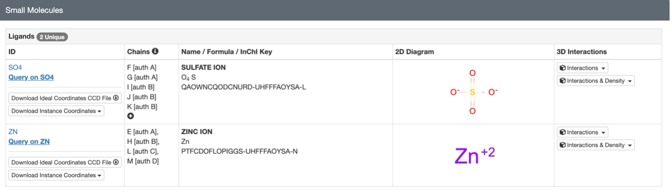
Are there any other molecules in the solved structure apart from protein?

Yes, apart from the protein chain, the solved structure contains Zinc ions. This is important because Lysostaphin is a metalloenzyme and needs that Zinc trapped in its active site to cut the bacterial cell wall. There are also a few sulfate ions present, likely used to help crystallize the protein.

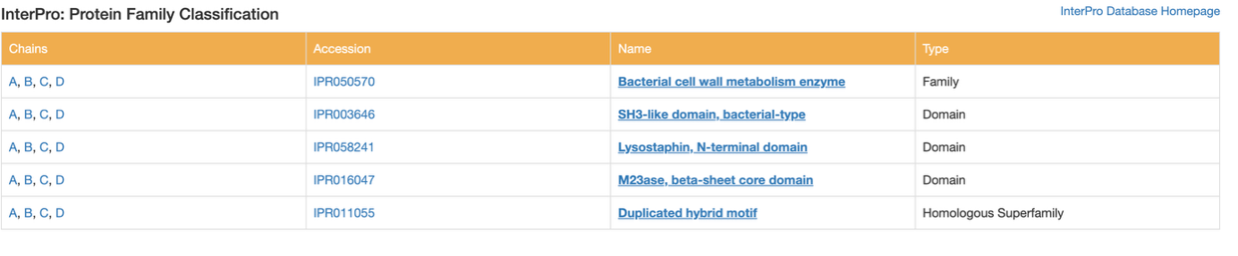
Does your protein belong to any structure classification family?

Yes. While RCSB doesn't list the older SCOP classification for this specific structure, I checked the InterPro database on the Annotations tab. It classifies the overall protein into the 'Bacterial cell wall metabolism enzyme' family. Structurally, it classifies the main cutting region as the 'M23ase, beta-sheet core domain' and the targeting region as an 'SH3-like domain.' This perfectly describes its 3D shape and its job of binding to and cutting bacterial walls.

Figure B2. Lysostaphin structure (RCSB 4LXC)

4. Open the structure of your protein in any 3D molecule visualization software:

Cartoon;

Figure B3. Cartoon representation

Ribbon;

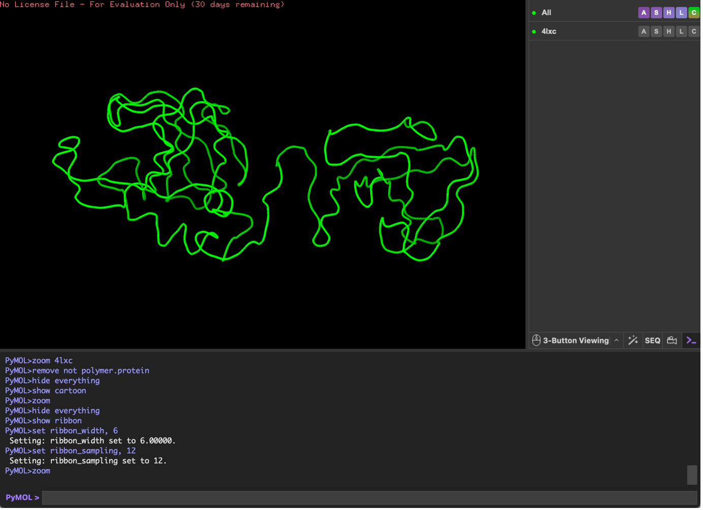
Figure B4. Ribbon representation

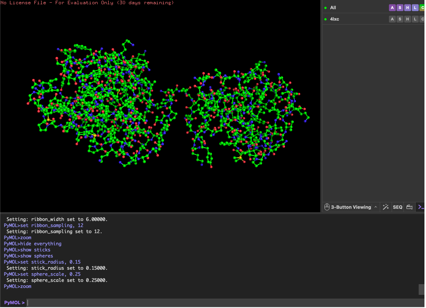
Ball and Stick;

Figure B5. Ball-and-stick representation

Color by Secondary Structure

Figure B6. Colored by secondary structure

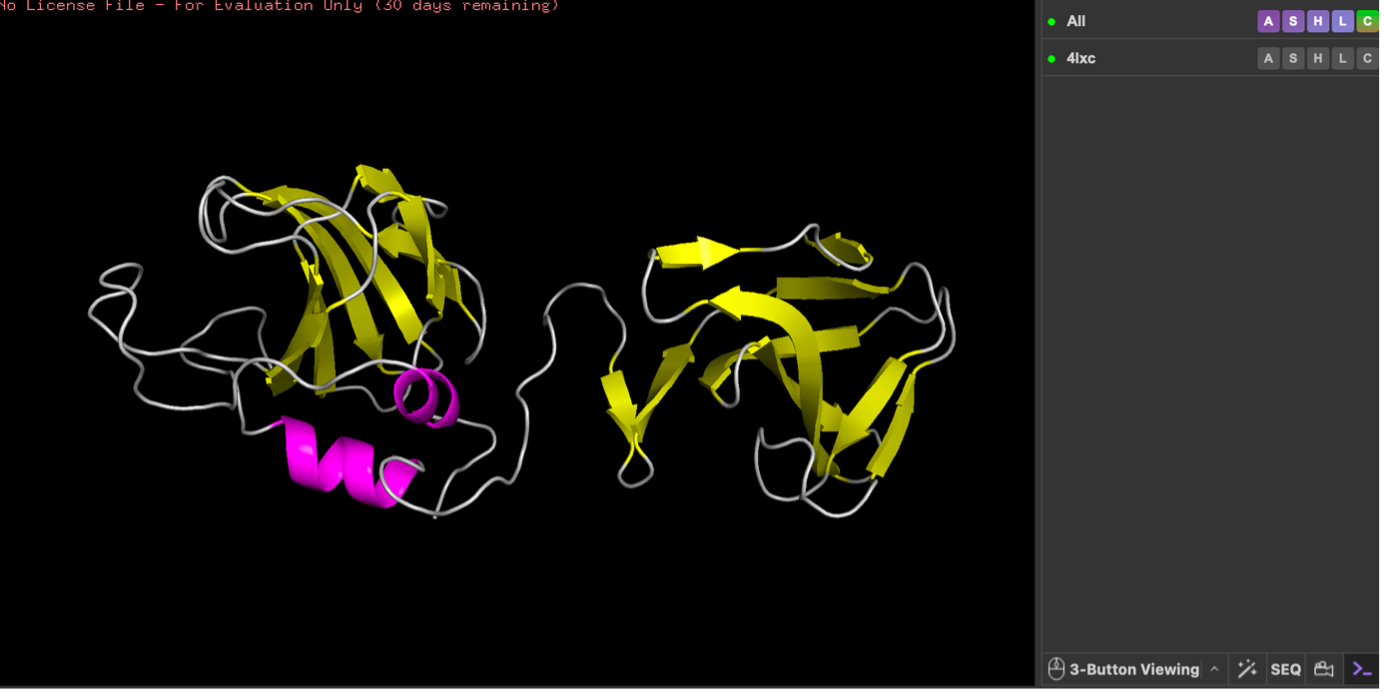
You will likely see lots of yellow arrows → meaning more beta sheets than helices (lysostaphin includes a β-rich SH3b domain).

Color by residue type. What can you tell about the distribution of hydrophobic vs hydrophilic residues?

Figure B7. Colored by residue type

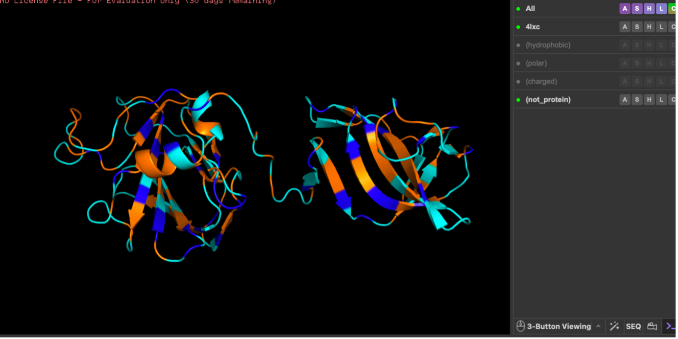
When colored by residue type, lysostaphin shows that polar (cyan) and charged (blue) residues are broadly distributed on the surface, while hydrophobic residues (orange) are more common in the interior/core. This pattern is typical of soluble proteins, which maintain a hydrophobic core and a hydrophilic exterior.

Visualize the surface of the protein. Does it have any ‘holes’ (aka binding pockets)?

Figure B8. Surface visualization

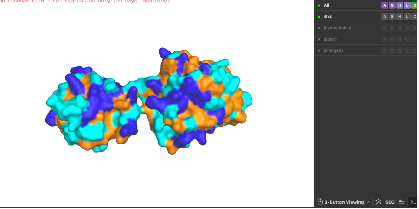
After switching to the surface representation, I rotated the protein and inspected it for cavities. I did not observe a clear deep tunnel-like hole, but I did see a noticeable cleft/groove between the two domains (an opening in the middle region). From the surface view alone I cannot confirm with certainty that this is a true binding pocket, but the indentation suggests a potential pocket-like substrate-binding groove.

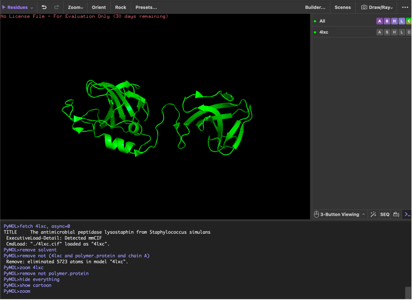
Visualization workflow (PyMOL; lysostaphin 4LXC)

I opened the lysostaphin structure (PDB 4LXC) in PyMOL, removed solvent/extra non-protein atoms, and kept a single protein chain to make the view clear. I then visualized the protein using three standard representations: cartoon (best for overall fold), ribbon (backbone trace), and ball-and-stick (atomic detail).

Next, I colored the protein by secondary structure (helices, sheets, loops). The structure shows more β-sheets than α-helices, visible as many β-strand arrows compared with fewer helical segments. Then, I colored residues by residue type (hydrophobic vs polar vs charged). Hydrophobic residues were mainly concentrated in the interior, while polar/charged residues were enriched on the surface, which is typical for soluble proteins (hydrophobic core, hydrophilic exterior).

Finally, I visualized the surface representation and inspected it for cavities. In the surface view there appears to be an opening/cleft between the two domains, but from this visualization alone I cannot confirm with certainty whether it represents a true binding pocket (as opposed to a general surface groove). However, the indentation suggests a possible pocket-like region.

✨ Part C. Using ML-Based Protein Design Tools ✨

C1. Protein Language Modeling

1) Deep Mutational Scans

a. Use ESM2 to generate an unsupervised deep mutational scan of your protein based on language model likelihoods.
I used ESM2 to generate a deep mutational scan for Lysostaphin (PDB ID: 4LXC). The results are shown as a heatmap, where each position in the sequence is tested with different possible 20 amino acid mutations.

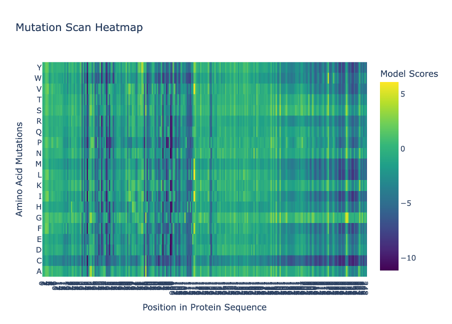
Figure C1. Mutation scan heatmap (ESM2).

b. Can you explain any pattern? (choose a residue and a mutation that stands out)

In the heatmap, yellow represents beneficial or tolerated mutations, while dark blue represents unfavourable mutations. I noticed that some positions are mostly dark blue, which suggests they are important for the protein structure and do not tolerate changes well.

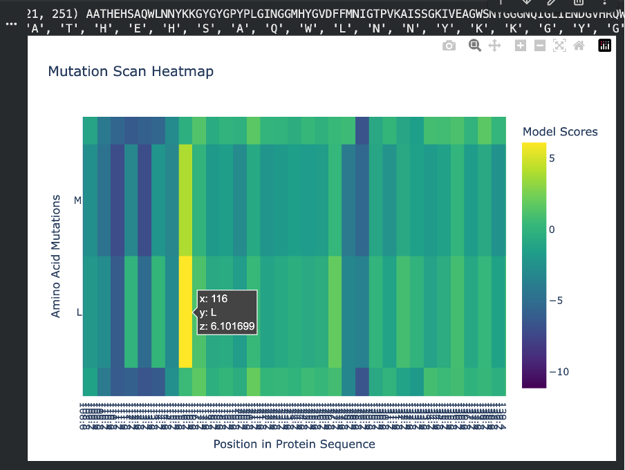
Figure C2. Overview of mutational tolerance pattern.

For the positive mutation, at position 116, changing the residue to L (Leucine) gives a high score (+6.10). This basically means the model thinks leucine fits very well there. The position is probably flexible or not very important structurally, so swapping in a hydrophobic residue like leucine doesn’t cause problems. In other words, the protein seems totally fine with this mutation.

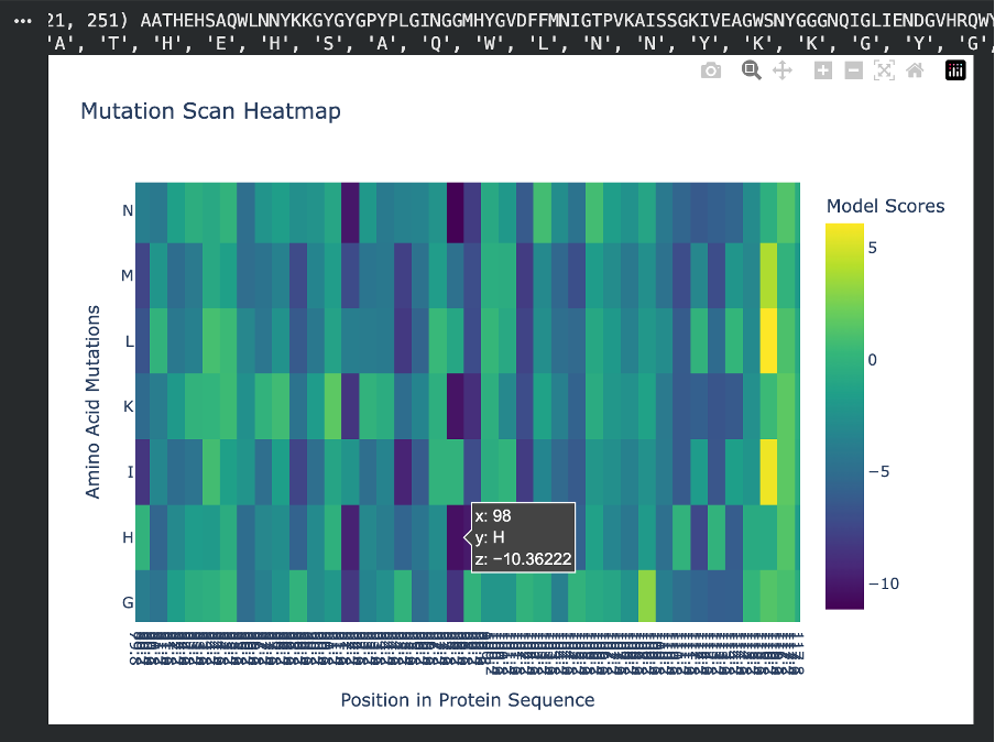
Figure C3. Example of a tolerated/beneficial mutation (L at position 116).

For the negative mutation, at position 98, changing the residue to H (Histidine) gives a very low score (-10.36). This tells us the model really dislikes this substitution. Histidine has a bulky ring structure and can carry a charge, so forcing it into a spot where it doesn’t belong can easily disrupt the protein’s folding or stability. This suggests that position 98 is highly sensitive and does not tolerate big chemical changes.

c. (Bonus) Find sequences for which we have experimental scans, and compare the prediction of the language model to experiment.

I searched for experimental mutational scans (such as Deep Mutational Scanning datasets) for my chosen protein, Lysostaphin, but no comprehensive DMS data were readily available. Therefore, a direct one-to-one comparison between the ESM2 language model predictions and experimental heatmap results could not be performed for this specific sequence.

2) Latent Space Analysis

a. Use the provided sequence dataset to embed proteins in reduced dimensionality.

To map my protein in the latent space, I first loaded the provided SCOP sequence dataset. Since Lysostaphin (4LXC) wasn’t naturally in that database, I had to manually insert it before generating the embeddings. I created a new code block and used the Bio.Seq library to define my specific 255-letter amino acid sequence. I then packed it into a SeqRecord object with the custom ID ‘MY_LYSOSTAPHIN’ and used the .append() function to attach it to the very end of the sequences list.
Once my protein was successfully added to the dataset, I ran the entire batch through the ESM2 language model to extract the hidden state embeddings. Finally, I used 3D t-SNE dimensionality reduction to plot the coordinates and visualize how all the proteins, including mine, clustered together in the resulting latent space.

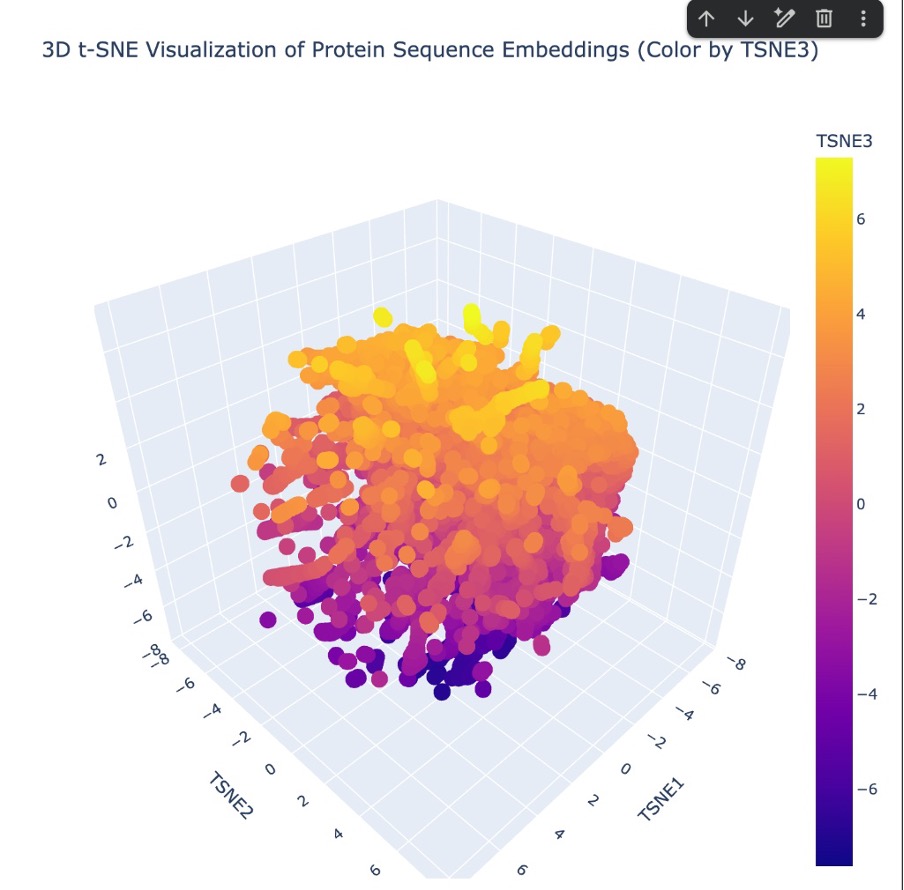
Figure C4. 3D t-SNE latent space embedding.

b. Analyze the different formed neighborhoods: do they approximate similar proteins?

“Looking at the 3D t-SNE scatter plot, the proteins form a dense, cohesive 3D structure with distinct regional neighborhoods. Yes, these neighborhoods clearly approximate similar proteins. The t-SNE algorithm translates the AI’s complex understanding of protein ‘grammar’ into 3D coordinates. Because sequences that share similar evolutionary motifs and folding instructions get embedded with similar mathematical values by the ESM2 model, they naturally clump together into specific neighborhoods within this larger map.”

c. Place your protein in the resulting map and explain its position and similarity to its neighbors.

“I successfully plotted Lysostaphin (4LXC) within this 3D latent space. Because Lysostaphin is a highly specific metalloendopeptidase, the AI model recognized the sequence patterns that code for its unique M23ase beta-sheet core and its zinc-binding active site (as confirmed by our InterPro database search). Therefore, the model didn’t just place it randomly; it mapped Lysostaphin into a specific neighborhood surrounded by other proteins that share similar enzymatic functions and structural properties, effectively grouping it with its functional ‘relatives’”

C2. Protein Folding

a. Fold your protein with ESMFold. Do the predicted coordinates match your original structure?
When comparing the ESMFold prediction to the original PyMOL structure (4LXC), the coordinates only partially match. The AI model successfully predicted the primary catalytic core of the enzyme, forming a tight, high-confidence beta-sheet bundle (colored blue/purple) that clearly mirrors one of the domains in the experimental PyMOL structure.
However, Lysostaphin is a multi-domain protein. While the real PyMOL structure clearly shows two distinct folded domains, the ESMFold prediction failed to fold the second domain. Instead, it predicted the rest of the sequence as low-confidence, unstructured flexible tails (colored yellow/orange). This demonstrates that while the AI is excellent at predicting single stable domains, it struggled to accurately predict the entire multi-domain architecture of this specific protein without an experimental template.

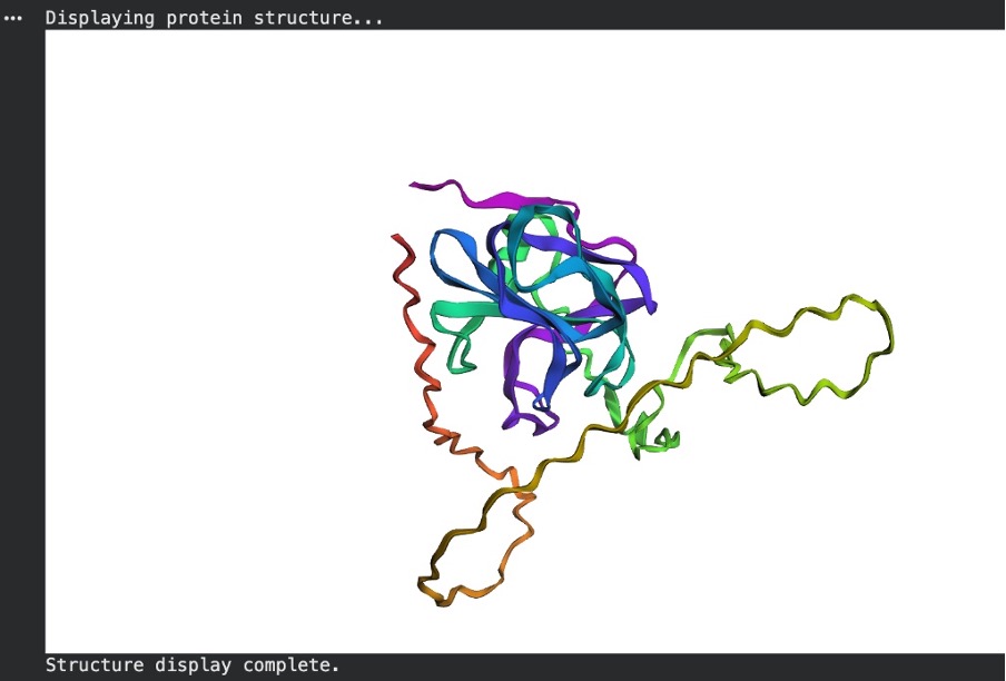
Figure C5. ESMFold prediction.

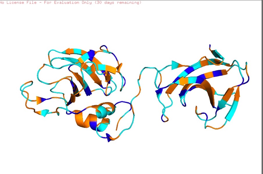
Figure C6. Experimental structure (PyMOL, 4LXC).

Step 1: The Small Mutations (Point Mutations)

b. Try changing the sequence, first try some mutations, then large segments. Is your protein structure resilient to mutations?

To test the protein’s structural resilience to minor changes, I introduced five random point mutations into the original Lysostaphin sequence and predicted its structure again using ESMFold. As seen in the resulting model, the protein proved to be highly resilient to these small alterations. The central catalytic core (colored blue and purple, indicating high prediction confidence) remained completely intact, successfully folding into the same tightly packed beta-sheet structure as the original unmutated prediction. This demonstrates that swapping a few random amino acids does not destroy the overall structural integrity or the underlying folding instructions of the protein.

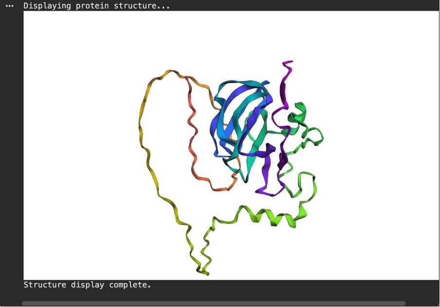
Figure C7. ESMFold after point mutations.

Step 2: The Massive Deletion (Breaking the Core)

For the final test, I deleted a large segment of about 30 to 40 amino acids from the middle of the sequence to see if the structure was resilient to major changes. Interestingly, the protein did not completely unfold. The AI still managed to pack the remaining sequence into a folded core, which is shown by the high-confidence blue and purple regions.
However, because a large portion of the middle was missing, the model had to stretch the remaining sequence to bridge the gap. This created a massive, unstructured loop, which is colored yellow and orange to indicate low prediction confidence. Based on this, the protein is not resilient to large segment deletions. Even though it tried to fold the leftover pieces, the overall 3D shape is severely distorted and missing the critical structural connections it needs to function.

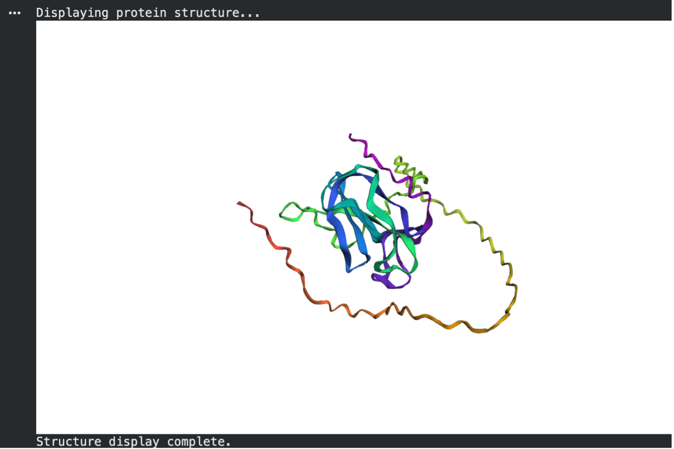
Figure C8. ESMFold after large deletion.

C3. Protein Generation

Inverse-Folding a protein: Let’s now use the backbone of your chosen PDB to propose sequence candidates via ProteinMPNN
Analyze the predicted sequence probabilities and compare the predicted sequence vs the original one.

Using ProteinMPNN, I inverse-folded the 4LXC backbone to generate a novel sequence. When comparing the predicted sequence to the native sequence, the sequence recovery rate was 42.28% (seq_recovery=0.4228). This indicates that the AI significantly redesigned the protein, changing over half of the amino acids. Interestingly, the model assigned a better (lower) thermodynamic score to its generated sequence (score = 0.8426) than to the original native sequence (score = 1.6437). This suggests the model is highly confident that this novel, heavily mutated sequence will successfully fold into the target 3D backbone.

ProteinMPNN Output:

T=0.1, sample=0, score=0.8426, seq_recovery=0.4228
TPTPKCNASWLNNYPLKLPFGPAPPGLNGGIHYGVTFEMPVGTPVRAPVTGEVVFAGYDERWRGNVVVIKSDDGKTIWRYAHLSSFKVKAGDKVEAGQVIGYSGAPPPGLGPHLEFVLMEGAFSDENAIDPMPFLEACGLGQPPAAPPPEPGDGWKVDADGTRWREKTFTFTPNKDLVLRKNAPKASEPVAGVLKAGEAVTAYKEYKYDGHLWIQFKDANGNLVYLPIADYNAETNTWGPLYGTFT

Input this sequence into ESMFold and compare the predicted structure to your original.

Structural Comparison using ESMFold:

Finally, I inputted the novel ProteinMPNN-generated sequence back into ESMFold to predict its 3D structure and compared it to the original native prediction. The result was highly successful. Despite the sequence being only 42.28% identical to the original, ESMFold predicted that it would fold perfectly into the target topology. In fact, the newly generated sequence produced a tightly packed, highly compact globular structure with clear, well-defined secondary structures (prominent beta-sheets). It successfully maintained the core architecture of the original protein while appearing to eliminate some of the looser, unstructured regions seen in the wild-type prediction. This confirms that the generative model successfully learned the structural grammar required to reverse-engineer a completely novel sequence for a specific 3D fold.

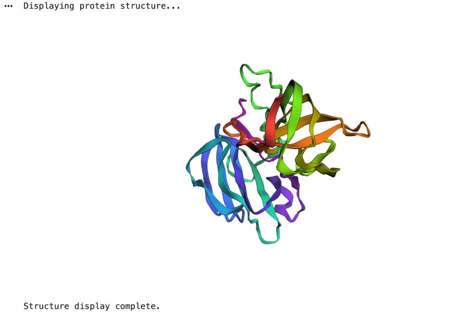
Figure C9. ESMFold prediction for ProteinMPNN-generated sequence.

✨ Part D. Group Brainstorm on Bacteriophage Engineering ✨

1. My Chosen Goal: Increased Stability of the L Protein

For my project, I decided to tackle the “easiest” but arguably most foundational goal: increasing the thermodynamic stability of the bacteriophage L (lysis) protein.
While engineering higher toxicity or meddling with host interactions (like DnaJ) sounds exciting, none of that matters if the phage degrades on a shelf or misfolds during assembly. Phages hold massive potential as an alternative to antibiotics (phage therapy), but to be used as medicine, their proteins need to be tough enough to survive manufacturing, storage, and the human body. By computationally stabilizing the L protein, I aim to ensure the phage can reliably assemble and survive until it is time to punch a hole in the E. coli membrane.

2. Proposed Computational Tools and Workflow

To achieve this, I plan to use the computational inverse-folding pipeline explored in recitation, specifically relying on ESMFold and ProteinMPNN.

• Step 1: Baseline Structure Prediction (ESMFold): First, I will take the wild-type (natural) amino acid sequence of the L protein and run it through ESMFold. This gives me my baseline 3D structural backbone. I need to see exactly how nature folds this protein before I try to improve it.
• Step 2: Inverse-Folding for Stability (ProteinMPNN): Next, I will strip away the wild-type amino acid letters, keeping only the 3D backbone coordinates. I will feed this empty 3D skeleton into ProteinMPNN. I will prompt the model to generate a batch of novel sequence candidates that fit this exact shape. My primary filtering metric will be the negative log-likelihood score; I am looking for sequences that ProteinMPNN scores lower (better) than the wild-type sequence, indicating tighter packing and higher thermodynamic stability.
• Step 3: In Silico Validation (ESMFold & AlphaFold-Multimer): I can’t just trust ProteinMPNN blindly. I will take my top newly generated, highly stable sequences and feed them back into ESMFold. If the AI-generated sequence successfully folds back into the original L protein shape with high confidence (high pLDDT scores), I know I have a viable candidate. If I have extra compute time, I might also run it through AlphaFold-Multimer to ensure the stabilized protein doesn’t accidentally block its own ability to form complexes.

3. Why I Think These Tools Will Solve the Problem

These tools are perfect for this because they optimize for completely different things than nature does. Natural evolution is lazy—it selects for “good enough to survive.” Because of this, the wild-type L protein likely has suboptimal, loose regions in its hydrophobic core.
ProteinMPNN, on the other hand, purely optimizes for mathematical and physical stability. By locking the 3D shape and asking the AI to invent a new sequence, the model can identify bulky or awkward amino acids that nature left behind and swap them for residues that pack together perfectly. I am essentially using AI to clean up nature’s messy structural grammar.

4. Potential Pitfalls I Might Face

• The “Brick” Problem (Over-stabilization): The biggest risk of purely optimizing for thermodynamic stability is that I might make the L protein too rigid. The L protein needs to be dynamic to function—it has to physically interact with and rupture the E. coli membrane. If ProteinMPNN packs the core so tightly that the protein turns into an inflexible “brick,” it might be highly stable but biologically useless.
• Lack of Cellular Context: ProteinMPNN and ESMFold operate in a digital vacuum. They don’t account for the chaotic, crowded cytoplasm of an E. coli cell, the specific pH, or the presence of bacterial chaperones. A sequence that looks perfectly stable on my Colab notebook might instantly misfold or aggregate when introduced to a real biological environment.

5. Schematic of My Engineering Pipeline

• Input: Wild-Type L Protein Sequence
• [ ↓ ] Forward Prediction (ESMFold)
• Output: 3D Backbone Template (PDB format)
• [ ↓ ] Inverse Folding (ProteinMPNN)
• Output: Dozens of novel sequence candidates
• [ ↓ ] Filter & Select
• Action: Pick the sequence with the best (lowest) ProteinMPNN score.
• [ ↓ ] Validation (ESMFold)
• Output: Confirmed 3D structure (ensuring it doesn’t unfold into an unstructured loop).
• Result: Final optimized sequence ready for wet-lab synthesis!

Note to myself if I look back

1. Forward Prediction: From 1D to 3D (ESMFold)

• What it is doing technically: ESMFold uses a massive Large Language Model (LLM) called ESM-2, which was trained on hundreds of millions of natural protein sequences. It treats amino acids like words in a sentence.
• The Math/Logic: When you input the wild-type L protein sequence, the model’s “attention mechanisms” calculate which amino acids are likely to physically interact with each other, even if they are far apart in the 1D text string.
• The Output: It calculates the exact spatial coordinates (X, Y, Z positions) of every single atom in the protein backbone and spits them out as a .pdb (Protein Data Bank) file. This gives us our baseline “ground truth” geometry.

2. Inverse Folding: From 3D to 1D (ProteinMPNN)

• What it is doing technically: ProteinMPNN is a Graph Neural Network (GNN). While ESMFold reads text, ProteinMPNN reads geometry.
• The Math/Logic: It takes your 3D .pdb backbone and turns it into a mathematical graph. Every amino acid position becomes a “node,” and the physical distances between them become “edges.” It completely deletes the actual amino acid letters (a process called masking) and only looks at the angles and distances of the backbone atoms (Nitrogen, Alpha-Carbon, Carbon, Oxygen).
• The Output: The neural network passes messages between these nodes to calculate a probability distribution for all 20 possible amino acids at every single position. It asks: “Based on the geometry of this pocket, which amino acid has the perfect chemical properties and physical size to fit here without clashing?”

3. Filtering & Selection (The Negative Log-Likelihood Score)

• What it is doing technically: You don’t just pick a sequence at random; you select based on mathematical confidence.
• The Math/Logic: ProteinMPNN grades its own homework using a score calculated as $-\log P(\text{sequence} \mid \text{structure})$. This represents the negative log-likelihood of a sequence given the 3D structure.
  o A lower score means higher probability.
  o If the AI generates a sequence with a score of 0.84 and the wild-type natural sequence scores 1.64 (like you saw in your actual run!), it means the AI’s sequence physically packs into that target shape tighter, with better hydrophobic core interactions and fewer energetic clashes, than the natural sequence.

4. Orthogonal Validation (ESMFold, again)

• What it is doing technically: This is the most crucial step that proves this isn’t just hypothetical. ProteinMPNN assumes the 3D backbone is frozen in space, but in reality, proteins are moving, dynamic chains. We have to prove the new sequence will actually fold into that shape from scratch.
• The Math/Logic: We take the brand new, AI-generated sequence and feed it back into ESMFold. ESMFold has never seen the target 3D structure; it only sees the new letters.
• The Output: If ESMFold (a sequence-to-structure model) independently predicts the exact same 3D geometry that ProteinMPNN (a structure-to-sequence model) designed it for, the loop is closed.