The Project Concept: Integrated Plant-Based Bone Scaffolds
The field of regenerative medicine currently relies heavily on static bone scaffolds that provide structural support but lack the ability to interact with the biological environment. I propose the development of a 3D bioprinted smart scaffold designed from sustainable, plant-based materials. This system will serve a dual purpose by providing a physical matrix for bone growth and integrating biosensors for real-time physiological monitoring. By using materials like alginate or cellulose, this approach offers a personalized and environmentally responsible alternative to traditional synthetic implants.
Technical Phases:
• Phase 1: Structural Foundation. The scaffold is bioprinted using biodegradable plant polymers tailored to the specific geometry of a patient’s bone defect. This provides the necessary mechanical integrity to support new tissue formation.
• Phase 2: Biological Intelligence. Biosensors are embedded within the matrix to monitor variables such as pH levels, calcium concentration, and mechanical strain. Simultaneously, a controlled delivery system releases growth factors to promote rapid vascularization and bone density.
• Phase 3: Controlled Degradation. As natural bone tissue regenerates and takes over the load-bearing responsibilities, the scaffold undergoes programmed biodegradation. This leaves behind only healthy, natural bone without the need for secondary surgeries to remove permanent hardware.
Governance Goals for Ethical Bioengineering
To ensure this technology aligns with safety and ethical standards, the following governance goals have been established.
Goal A: Environmental Sustainability and Non-Toxicity
The project must ensure that the transition to plant-based materials does not result in unintended ecological or biological consequences.
• Sub-goal: Utilize biodegradable materials that break down into inert metabolites to avoid systemic toxicity.
• Sub-goal: Standardize sourcing methods to ensure that plant extraction does not disrupt local ecosystems or biodiversity.
Goal B: Clinical Efficacy and Patient Protection
The integration of active growth factors requires strict oversight to prevent adverse biological reactions.
• Sub-goal: Validate the biocompatibility of all plant-derived components to eliminate the risk of chronic inflammation or immune rejection.
• Sub-goal: Implement precise delivery protocols for growth factors to prevent unregulated cellular proliferation.
Proposed Governance Actions
Action 1: Regulatory Frameworks for Bio-Hybrid Materials
The primary purpose is to establish clear safety benchmarks for plant-based medical devices that do not fit into existing regulatory categories. This involves collaboration with the MHRA and FDA to define specific testing protocols for the degradation rates of cellulose-based implants. The design of this action requires rigorous longitudinal studies to confirm that the breakdown of these materials is safe over several years. One significant risk is that high regulatory hurdles may delay the delivery of these life-changing treatments to patients in need.
Action 2: Data Security Protocols for In-Vivo Biosensors
As these scaffolds generate continuous streams of patient health data, it is vital to establish ethical data handling practices. The design of this action includes the development of encrypted transmission standards to ensure that sensitive biological information is only accessible to authorized medical personnel. A key assumption is that patient data can be transmitted wirelessly without compromising the physical integrity of the scaffold. The risk of failure involves potential cybersecurity vulnerabilities that could expose private health metrics.
Action 3: Global Sustainability Certification
This action focuses on creating a “Green Biotech” certification to encourage the use of eco-friendly materials in the medical industry. By working with the United Nations Environment Programme, we can set international standards for the carbon footprint of medical manufacturing. This assumes that a global market exists for sustainable medical products. However, a potential risk is that the cost of obtaining such certifications could increase the final price of the scaffold, potentially limiting access for lower-income healthcare systems.
Scoring of Governance Actions
Evaluation Criteria Action 1: Regulation Action 2: Data Privacy Action 3: Certification
Enhance Biosecurity 1 2 3
Foster Lab Safety 1 3 2
Protect the Environment 2 3 1
Stakeholder Feasibility 2 2 1
Constructive Application 1 2 1
(Note: 1 represents the highest alignment with the goal)
Prioritization and Ethical Considerations
Upon reviewing the scores, Action 1 (Regulation of Biodegradable Biomaterials) is the highest priority. Without a validated safety profile and regulatory approval, the clinical and environmental benefits of the scaffold cannot be realized. While Action 3 is easier to implement, it remains secondary to the fundamental safety of the patient.
During the development of this proposal, an important ethical concern arose regarding “Biotelemetry Equity.” If smart scaffolds become the gold standard, there is a risk that only patients in high-resource settings will benefit from real-time healing monitoring. To address this, governance actions should include incentives for companies to develop “passive” versions of the scaffold that provide high-quality structural support at a lower cost for global distribution.
Relevant Audiences
The recommendations for these governance actions are directed toward the FDA and the World Health Organization. These bodies are essential for establishing the international safety and sustainability standards required to bring 3D bioprinted plant-based scaffolds into mainstream clinical practice.
Q1: Even though it is not perfect, the precision of nature’s machinery for copying DNA is actually quite staggering. The intrinsic error rate of DNA polymerase is approximately one mistake for every million base pairs copied (10^(−6)). For context, the human genome comprises around 3.2 billion base pairs. If we were to depend solely on polymerase, each and every cell division would give rise to innumerable arbitrary mutations. This would have catastrophic consequences for the stability of life over many generations, but biology handles this massive discrepancy through a multi-layered proofreading and repair system. First, the polymerase itself has a ‘delete’ function whereby it can sense a mismatch, back up and correct it. Secondary systems, such as the MutS repair complex, then scan the DNA afterwards to detect any rare mistakes that have slipped through the first net. This combined effort brings the final error rate down to approximately one in a billion. This makes it reliable enough to maintain the blueprint of a human being.
Q2: When it comes to coding proteins, there is an incredible amount of flexibility because the genetic code is redundant. Since most amino acids are linked to several different three letter codons, you could theoretically write the DNA sequence for an average human protein in more ways than there are atoms in the universe. In practice, however, most of these sequences just do not work in a living cell. A major reason for this is the physical shape the RNA takes. If a sequence accidentally folds into a tight hairpin or a complex secondary structure, the cellular machinery gets physically stuck, much like a zipper hitting a snag in fabric. There are also issues with sequences having extreme GC ratios, which makes them too unstable or difficult for the cell to handle. Plus, cells have internal “cleavage rules” where they recognize certain patterns as signals to chop up the genetic instructions before they can even be translated. So, while the theoretical options are infinite, the actual biological grammar needed to express a protein is much more restrictive.
Questions from Dr. LeProust
Q1: The standard approach is the phosphoramidite method, which follows a four-step cycle. It starts with coupling the phosphoramidite to the chain, followed by capping any unreacted sites to prevent errors. The link is then oxidized to stabilize it, and finally, the growing chain is deblocked to prepare it for the next nucleotide addition.
Q2: The main issue is the cumulative effect of coupling efficiency. Even with a very high success rate for each step, small errors add up quickly over many cycles. By the time you reach 200 nucleotides, these compounding errors and the accumulation of truncated or incorrect sequences make it nearly impossible to retrieve a pure, full-length product.
Q3: Synthesizing a 2000bp gene directly would require 2000 consecutive coupling cycles without a single mistake, which is chemically unrealistic with current technology. The yield of the correct full-length molecule would be effectively zero. Beyond the chemistry, the sheer cost and the buildup of chemical damage over such a long process make it much more practical to assemble smaller fragments rather than trying to print the whole gene at once.
The ten amino acids that are generally considered to be essential for animals are: arginine, histidine, isoleucine, leucine, lysine, methionine, phenylalanine, threonine, tryptophan and valine. They are classified as essential because animals cannot synthesise sufficient quantities of their carbon skeletons, meaning they must be obtained through diet or from symbiotic relationships with microbes.
Questions from George Church
The ’lysine contingency’ refers to the fact that animals have lost the ability to produce lysine independently. From an evolutionary perspective, this seems less like a biological flaw and more like a way for ecosystems to create a reliance between different species. Our specific need for this amino acid has shaped the world as we know it, creating massive agricultural systems and complex food webs that would not exist if we could produce lysine ourselves. For example, the industrial production of lysine for livestock feed is a significant global enterprise centred on optimising animal growth. Without this essential amino acid, the entire economic and agricultural infrastructure might not exist, and we might not have moved towards such extensive farming practices. I wonder if, over millions of years, animals became dependent on lysine as a kind of self-imposed evolutionary trade-off. Perhaps it was once non-essential, but because it was so abundant in the environment, our ancestors eventually ’turned off’ the expensive metabolic machinery needed to produce it. In that sense, what we call a contingency is really just nature’s efficient way of outsourcing production to the surrounding environment.
References;
Part1: Assignment 1. The Project Concept: Integrated Plant-Based Bone Scaffolds The field of regenerative medicine currently relies heavily on static bone scaffolds that provide structural support but lack the ability to interact with the biological environment. I propose the development of a 3D bioprinted smart scaffold designed from sustainable, plant-based materials. This system will serve a dual purpose by providing a physical matrix for bone growth and integrating biosensors for real-time physiological monitoring. By using materials like alginate or cellulose, this approach offers a personalized and environmentally responsible alternative to traditional synthetic implants.
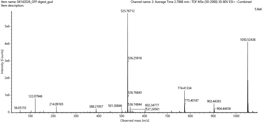
✨Part 1: Benchling & In silico Gel Art I simulated a restriction digest on λ DNA in Benchling using enzymes like EcoRI, HindIII, and BamHI, EcoRV, Kpnl. By comparing the band patterns, I could visualize how different enzymes cut the DNA into fragments of varying sizes. This simulation helped me understand how we verify DNA fingerprints before moving to synthesis.
Week 3 – Lab Automation ✨ Week 3 - Homework ✨ You can view my Automation Art design here: Opentrons Art Link
After creating this shell pattern using Opentrons Art, I duplicated the provided Colab notebook to develop a Python protocol. To program the Opentrons robot to physically recreate the artwork on a plate, I systematically entered the coordinate data from my design step-by-step into the script. Once the protocol was complete, it successfully generated the images shown below.
WEEK 4 — PROTEIN DESIGN PART I ✨ Part A. Conceptual Questions ✨ 1. How many molecules of amino acids do you take with a piece of 500 grams of meat? (on average an amino acid is ~100 Daltons)
Let’s walk through the math by looking directly at the weight. We know an average amino acid is about 100 Daltons. If we convert that to grams, one single Dalton is an incredibly tiny fraction of a gram (about 1.66 × 10⁻²⁴ g). That means our single 100-Dalton amino acid weighs roughly 1.66 × 10⁻²² grams. If we have a 500-gram piece of meat and we pretend for a second that it is 100% pure protein, we just divide the total weight by the weight of one molecule. So, 500 g divided by 1.66 × 10⁻²² g/molecule gives us roughly 3.01 × 10²⁴ amino acid molecules.
✨ Part A. SOD1 Binder Peptide Design ✨ Part 1: Generate Binders with PepMLM Sequence Retrieval and Mutation I began by retrieving the human Superoxide dismutase 1 (SOD1) sequence from the UniProt database using the accession number P00441. The native (wild-type) sequence consists of 154 amino acids:
MATKAVCVLKGDGPVQGIINFEQKESNGPVKVWGSIKGLTEGLHGFHVHEFGDNTAGCTSAGPHFNPLSRKHGGPKDEERHVGDLGNVTADKDGVADVSIEDSVISLSGDHCIIGRTLVVHEKADDLGKGGNEESTKTGNAGSRLACGVIGIAQ
To model the disease state, I introduced the ALS-causing A4V mutation (Alanine → Valine at residue 4). Noting that standard numbering excludes the initiator Methionine (M), I replaced the Alanine at the 5th position with a Valine to create my target mutant sequence:
✨ DNA Assembly ✨ Question 1: What are some components in the Phusion High-Fidelity PCR Master Mix and what is their purpose? Since the protocol didn’t list the exact ingredients, I looked up the standard components of a Phusion Master Mix from a supplier like New England Biolabs. A PCR Master Mix is basically a pre-mixed tube of everything needed to copy DNA, minus the specific template and primers. The main components are:
Assignment Part 1: Intracellular Artificial Neural Networks (IANNs) 1. What advantages do IANNs have over traditional genetic circuits? In my research, I found that IANNs offer a much more flexible way to handle biological data compared to standard Boolean (ON/OFF) circuits. Here are the main benefits:
HTGAA Week 9: Cell-Free Systems Part A: General and Lecturer-Specific Questions 1. Explain the main advantages of cell-free protein synthesis (CFPS) over traditional in vivo methods, specifically in terms of flexibility and control over experimental variables. Name at least two cases where cell-free expression is more beneficial than cell production. The biggest advantage I see is that CFPS turns “biology” into “chemistry.” In traditional in vivo systems, the cell membrane is a wall that prevents us from easily tweaking the internal environment. In a cell-free setup, I have an “open” system. I can add non natural amino acids, adjust salt concentrations (Mg²⁺ and K⁺) in real time, or even add detergents to help fold tricky proteins.
Homework: Final Project 1. Which aspect(s) of your project will you measure? The main goal is to measure how well my custom DNA construct actually stays stuck to the 3D-printed scaffold. I also need to measure the bioactivity of the produced protein — essentially checking if it actually triggers bone-growing signals like it’s supposed to. Finally, I’ll be measuring the retention time, which tells me how much longer my “anchored” version stays on the scaffold compared to a standard version that usually just washes away.
Week 11 — Bioproduction & Cloud Labs Part A: The 1,536 Pixel Artwork Canvas | Collective Artwork Make a note on your HTGAA webpages including:
(a) What you contributed to the community bioart project (e.g., “I made part of the DNA on the bottom right plate”) Honestly, I didn’t get to contribute a pixel this time. The window between the personalized URL going out and the editing deadline on Sunday 4/19 closed before I was able to sit down and place mine, which I’m a bit bummed about because the project sounded cool.
Integrated Plant-Based Bone Scaffolds
The field of regenerative medicine currently relies heavily on static bone scaffolds that provide structural support but lack the ability to interact with the biological environment. I propose the development of a 3D bioprinted smart scaffold designed from sustainable, plant-based materials. This system will serve a dual purpose by providing a physical matrix for bone growth and integrating biosensors for real-time physiological monitoring. By using materials like alginate or cellulose, this approach offers a personalized and environmentally responsible alternative to traditional synthetic implants.
Technical Phases:
• Phase 1: Structural Foundation. The scaffold is bioprinted using biodegradable plant polymers tailored to the specific geometry of a patient’s bone defect. This provides the necessary mechanical integrity to support new tissue formation.
• Phase 2: Biological Intelligence. Biosensors are embedded within the matrix to monitor variables such as pH levels, calcium concentration, and mechanical strain. Simultaneously, a controlled delivery system releases growth factors to promote rapid vascularization and bone density.
• Phase 3: Controlled Degradation. As natural bone tissue regenerates and takes over the load-bearing responsibilities, the scaffold undergoes programmed biodegradation. This leaves behind only healthy, natural bone without the need for secondary surgeries to remove permanent hardware.
2. Governance Goals for Ethical Bioengineering
To ensure this technology aligns with safety and ethical standards, the following governance goals have been established.
Goal A: Environmental Sustainability and Non-Toxicity
The project must ensure that the transition to plant-based materials does not result in unintended ecological or biological consequences.
• Sub-goal: Utilize biodegradable materials that break down into inert metabolites to avoid systemic toxicity.
• Sub-goal: Standardize sourcing methods to ensure that plant extraction does not disrupt local ecosystems or biodiversity.
Goal B: Clinical Efficacy and Patient Protection
The integration of active growth factors requires strict oversight to prevent adverse biological reactions.
• Sub-goal: Validate the biocompatibility of all plant-derived components to eliminate the risk of chronic inflammation or immune rejection.
• Sub-goal: Implement precise delivery protocols for growth factors to prevent unregulated cellular proliferation.
3. Proposed Governance Actions
Action 1: Regulatory Frameworks for Bio-Hybrid Materials
The primary purpose is to establish clear safety benchmarks for plant-based medical devices that do not fit into existing regulatory categories. This involves collaboration with the MHRA and FDA to define specific testing protocols for the degradation rates of cellulose-based implants. The design of this action requires rigorous longitudinal studies to confirm that the breakdown of these materials is safe over several years. One significant risk is that high regulatory hurdles may delay the delivery of these life-changing treatments to patients in need.
Action 2: Data Security Protocols for In-Vivo Biosensors
As these scaffolds generate continuous streams of patient health data, it is vital to establish ethical data handling practices. The design of this action includes the development of encrypted transmission standards to ensure that sensitive biological information is only accessible to authorized medical personnel. A key assumption is that patient data can be transmitted wirelessly without compromising the physical integrity of the scaffold. The risk of failure involves potential cybersecurity vulnerabilities that could expose private health metrics.
Action 3: Global Sustainability Certification
This action focuses on creating a “Green Biotech” certification to encourage the use of eco-friendly materials in the medical industry. By working with the United Nations Environment Programme, we can set international standards for the carbon footprint of medical manufacturing. This assumes that a global market exists for sustainable medical products. However, a potential risk is that the cost of obtaining such certifications could increase the final price of the scaffold, potentially limiting access for lower-income healthcare systems.
4. Scoring of Governance Actions
Evaluation Criteria
Action 1: Regulation
Action 2: Data Privacy
Action 3: Certification
Enhance Biosecurity
1
2
3
Foster Lab Safety
1
3
2
Protect the Environment
2
3
1
Stakeholder Feasibility
2
2
1
Constructive Application
1
2
1
(Note: 1 represents the highest alignment with the goal)
5. Prioritization and Ethical Considerations
Upon reviewing the scores, Action 1 (Regulation of Biodegradable Biomaterials) is the highest priority. Without a validated safety profile and regulatory approval, the clinical and environmental benefits of the scaffold cannot be realized. While Action 3 is easier to implement, it remains secondary to the fundamental safety of the patient.
During the development of this proposal, an important ethical concern arose regarding “Biotelemetry Equity.” If smart scaffolds become the gold standard, there is a risk that only patients in high-resource settings will benefit from real-time healing monitoring. To address this, governance actions should include incentives for companies to develop “passive” versions of the scaffold that provide high-quality structural support at a lower cost for global distribution.
Relevant Audiences
The recommendations for these governance actions are directed toward the FDA and the World Health Organization. These bodies are essential for establishing the international safety and sustainability standards required to bring 3D bioprinted plant-based scaffolds into mainstream clinical practice.
Q1: Even though it is not perfect, the precision of nature’s machinery for copying DNA is actually quite staggering. The intrinsic error rate of DNA polymerase is approximately one mistake for every million base pairs copied (10^(−6)). For context, the human genome comprises around 3.2 billion base pairs. If we were to depend solely on polymerase, each and every cell division would give rise to innumerable arbitrary mutations. This would have catastrophic consequences for the stability of life over many generations, but biology handles this massive discrepancy through a multi-layered proofreading and repair system. First, the polymerase itself has a ‘delete’ function whereby it can sense a mismatch, back up and correct it. Secondary systems, such as the MutS repair complex, then scan the DNA afterwards to detect any rare mistakes that have slipped through the first net. This combined effort brings the final error rate down to approximately one in a billion. This makes it reliable enough to maintain the blueprint of a human being.
Q2: When it comes to coding proteins, there is an incredible amount of flexibility because the genetic code is redundant. Since most amino acids are linked to several different three letter codons, you could theoretically write the DNA sequence for an average human protein in more ways than there are atoms in the universe. In practice, however, most of these sequences just do not work in a living cell. A major reason for this is the physical shape the RNA takes. If a sequence accidentally folds into a tight hairpin or a complex secondary structure, the cellular machinery gets physically stuck, much like a zipper hitting a snag in fabric. There are also issues with sequences having extreme GC ratios, which makes them too unstable or difficult for the cell to handle. Plus, cells have internal “cleavage rules” where they recognize certain patterns as signals to chop up the genetic instructions before they can even be translated. So, while the theoretical options are infinite, the actual biological grammar needed to express a protein is much more restrictive.
Questions from Dr. LeProust
Q1: The standard approach is the phosphoramidite method, which follows a four-step cycle. It starts with coupling the phosphoramidite to the chain, followed by capping any unreacted sites to prevent errors. The link is then oxidized to stabilize it, and finally, the growing chain is deblocked to prepare it for the next nucleotide addition.
Q2: The main issue is the cumulative effect of coupling efficiency. Even with a very high success rate for each step, small errors add up quickly over many cycles. By the time you reach 200 nucleotides, these compounding errors and the accumulation of truncated or incorrect sequences make it nearly impossible to retrieve a pure, full-length product.
Q3: Synthesizing a 2000bp gene directly would require 2000 consecutive coupling cycles without a single mistake, which is chemically unrealistic with current technology. The yield of the correct full-length molecule would be effectively zero. Beyond the chemistry, the sheer cost and the buildup of chemical damage over such a long process make it much more practical to assemble smaller fragments rather than trying to print the whole gene at once. The ten amino acids that are generally considered to be essential for animals are: arginine, histidine, isoleucine, leucine, lysine, methionine, phenylalanine, threonine, tryptophan and valine. They are classified as essential because animals cannot synthesise sufficient quantities of their carbon skeletons, meaning they must be obtained through diet or from symbiotic relationships with microbes.
Questions from George Church
The ’lysine contingency’ refers to the fact that animals have lost the ability to produce lysine independently. From an evolutionary perspective, this seems less like a biological flaw and more like a way for ecosystems to create a reliance between different species. Our specific need for this amino acid has shaped the world as we know it, creating massive agricultural systems and complex food webs that would not exist if we could produce lysine ourselves. For example, the industrial production of lysine for livestock feed is a significant global enterprise centred on optimising animal growth. Without this essential amino acid, the entire economic and agricultural infrastructure might not exist, and we might not have moved towards such extensive farming practices. I wonder if, over millions of years, animals became dependent on lysine as a kind of self-imposed evolutionary trade-off. Perhaps it was once non-essential, but because it was so abundant in the environment, our ancestors eventually ’turned off’ the expensive metabolic machinery needed to produce it. In that sense, what we call a contingency is really just nature’s efficient way of outsourcing production to the surrounding environment.
I simulated a restriction digest on λ DNA in Benchling using enzymes like EcoRI, HindIII, and BamHI, EcoRV, Kpnl. By comparing the band patterns, I could visualize how different enzymes cut the DNA into fragments of varying sizes. This simulation helped me understand how we verify DNA fingerprints before moving to synthesis.
✨ Part 3: DNA Design Challenge
3.1. Choose your protein
My Choice:
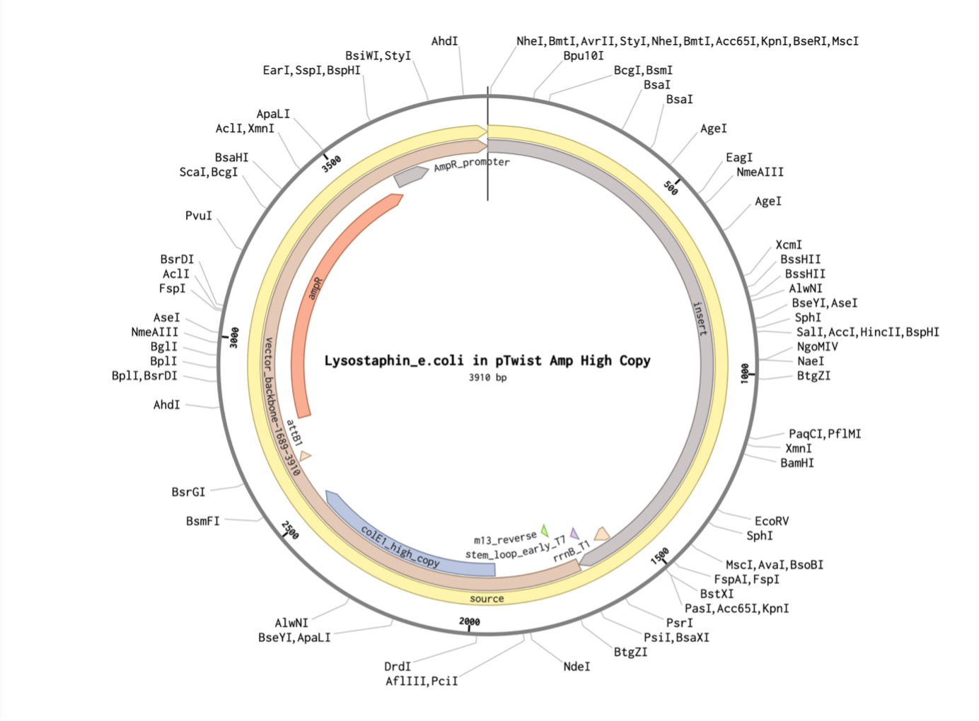
For this assignment, I chose Lysostaphin, a glycylglycine endopeptidase enzyme. This protein is naturally produced by Staphylococcus simulans to kill rival bacteria.
Why I chose it:
My background is in dentistry and tissue engineering, where peri-implantitis (infection around dental implants) is a critical failure mode. These infections are often caused by antibiotic-resistant Staphylococcus aureus (MRSA) forming biofilms on the titanium surface. Lysostaphin is capable of slicing through the cell wall of S. aureus, destroying the biofilm effectively where traditional antibiotics fail. It represents a potential “biological scalpel” for saving failing implants.
Sequence:
Using UniProt, I obtained the amino acid sequence for Lysostaphin:
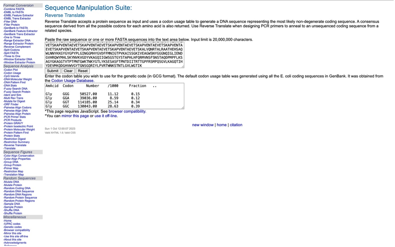
Using the online resource at https://www.bioinformatics.org/, I converted the amino acid sequence(taken from https://www.uniprot.org) of the Lysostaphin protein back into its potential DNA sequence. This technique follows the Central Dogma of Molecular Biology, which outlines the flow of genetic information from DNA to RNA and finally to protein. By reversing this sequence, the tool creates a logical nucleotide chain capable of producing that specific protein.
Converted Sequence:
reverse translation of Untitled to a 1479 base sequence of most likely codons.
atgaaaaaaaccaaaaacaactattatacccgcccgctggcgattggcctgagcaccttt
gcgctggcgagcattgtgtatggcggcattcagaacgaaacccatgcgagcgaaaaaagc
aacatggatgtgagcaaaaaagtggcggaagtggaaaccagcaaagcgccggtggaaaac
accgcggaagtggaaaccagcaaagcgccggtggaaaacaccgcggaagtggaaaccagc
aaagcgccggtggaaaacaccgcggaagtggaaaccagcaaagcgccggtggaaaacacc
gcggaagtggaaaccagcaaagcgccggtggaaaacaccgcggaagtggaaaccagcaaa
gcgccggtggaaaacaccgcggaagtggaaaccagcaaagcgccggtggaaaacaccgcg
gaagtggaaaccagcaaagcgccggtggaaaacaccgcggaagtggaaaccagcaaagcg
ccggtggaaaacaccgcggaagtggaaaccagcaaagcgccggtggaaaacaccgcggaa
gtggaaaccagcaaagcgccggtggaaaacaccgcggaagtggaaaccagcaaagcgccg
gtggaaaacaccgcggaagtggaaaccagcaaagcgccggtggaaaacaccgcggaagtg
gaaaccagcaaagcgccggtggaaaacaccgcggaagtggaaaccagcaaagcgctggtg
cagaaccgcaccgcgctgcgcgcggcgacccatgaacatagcgcgcagtggctgaacaac
tataaaaaaggctatggctatggcccgtatccgctgggcattaacggcggcatgcattat
ggcgtggatttttttatgaacattggcaccccggtgaaagcgattagcagcggcaaaatt
gtggaagcgggctggagcaactatggcggcggcaaccagattggcctgattgaaaacgat
ggcgtgcatcgccagtggtatatgcatctgagcaaatataacgtgaaagtgggcgattat
gtgaaagcgggccagattattggctggagcggcagcaccggctatagcaccgcgccgcat
ctgcattttcagcgcatggtgaacagctttagcaacagcaccgcgcaggatccgatgccg
tttctgaaaagcgcgggctatggcaaagcgggcggcaccgtgaccccgaccccgaacacc
ggctggaaaaccaacaaatatggcaccctgtataaaagcgaaagcgcgagctttaccccg
aacaccgatattattacccgcaccaccggcccgtttcgcagcatgccgcagagcggcgtg
ctgaaagcgggccagaccattcattatgatgaagtgatgaaacaggatggccatgtgtgg
gtgggctataccggcaacagcggccagcgcatttatctgccggtgcgcacctggaacaaa
agcaccaacaccctgggcgtgctgtggggcaccattaaa
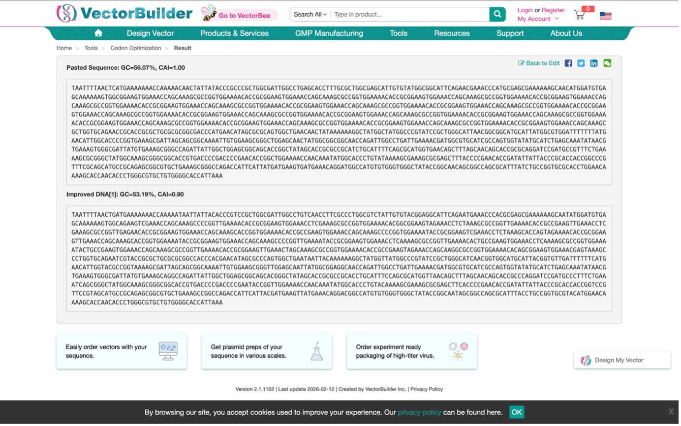
3.3. Codon optimization
Why do we optimize codons?
I need to ensure my DNA “reads” fluently in the host organism. If the codons are rare in the host, protein production will stall. Optimization replaces these rare codons with the host’s preferred ones without changing the final protein structure.
Which organism did you choose and why?
I chose Escherichia coli (E. coli) for codon optimization.
While my final application is for dental patients, E. coli is the industrial standard for manufacturing proteins. By optimizing for E. coli, I can grow large vats of bacteria, induce them to produce Lysostaphin, and then purify the enzyme to be applied as a dental gel or coating for implants.
Optimization Result:
3.4. You have a sequence! Now what?
Now that I have the optimized DNA sequence, the goal is recombinant protein production to create a therapeutic solution for peri-implantitis.
Cloning
I will insert the optimized Lysostaphin gene into an expression vector (plasmid). This plasmid acts as the delivery vehicle, containing a strong promoter that signals the host cell to begin producing the protein.
Transformation
The recombinant plasmid is put into $E. coli$ bacteria. This is achieved through a process called transformation (such as heat-shock), which allows the bacterial cells to take up the foreign DNA and host it within their own systems.
Expression
The bacteria act as biological factories, following the Central Dogma of Molecular Biology. The $E. coli$ cells read the optimized DNA instructions to produce mRNA via transcription, which is then translated into the Lysostaphin Protein. Because the codons were optimized for $E. coli$ (K12), the translation process is highly efficient with a high protein yield.
Purification
Finally, I will extract the protein from the bacterial culture. Through a series of filtration and chromatography steps, the Lysostaphin is isolated from other bacterial proteins. The result is a pure protein that can be formulated into a bioactive gel designed to target and eliminate $Staphylococcus$ biofilms in patients with peri-implantitis.
3.5. [Optional] How does it work in nature/biological systems?
Describe how a single gene codes for multiple proteins at the transcriptional level.
A gene is first transcribed into a long RNA molecule called pre-mRNA. This pre-mRNA contains both coding regions (exons) and non-coding regions (introns).
Through a process called Alternative Splicing, the cell can cut out the introns and stitch the exons together in different combinations. Just like editing a movie scene in different ways, different combinations of exons create different final mRNA molecules.
$$Different \ mRNA \ variants \rightarrow Different \ Proteins$$
Because the mRNA sequence changes, the resulting amino acid sequence changes too. This allows a single gene to code for multiple different protein isoforms, maximizing the efficiency of the genome.
Try aligning the DNA sequence, the transcribed RNA, and also the resulting translated Protein!
In nature, the enzyme RNA Polymerase reads the DNA template strand and synthesizes a single-stranded RNA molecule based on base complementarity.
• A pairs with U (Uracil replaces Thymine in RNA).
• T pairs with A.
• G pairs with C.
• C pairs with G.
After transcription, the Ribosome reads the mRNA in groups of three nucleotides called codons. Each codon corresponds to one specific amino acid.
Alignment for Lysostaphin (Start of Sequence):
Here is the flow of information for the first 6 amino acids of my Lysostaphin protein (MTTTPD…).
• DNA (Coding Strand): ATG ACC ACC ACC CCG GAT
• mRNA (Transcription): AUG ACC ACC ACC CCG GAU
• Protein (Translation): M T T T P D
Key:
• M (Methionine): The “Start” signal.
• T (Threonine): A polar amino acid.
• P (Proline): Adds structural rigidity.
• D (Aspartic Acid): Negatively charged.
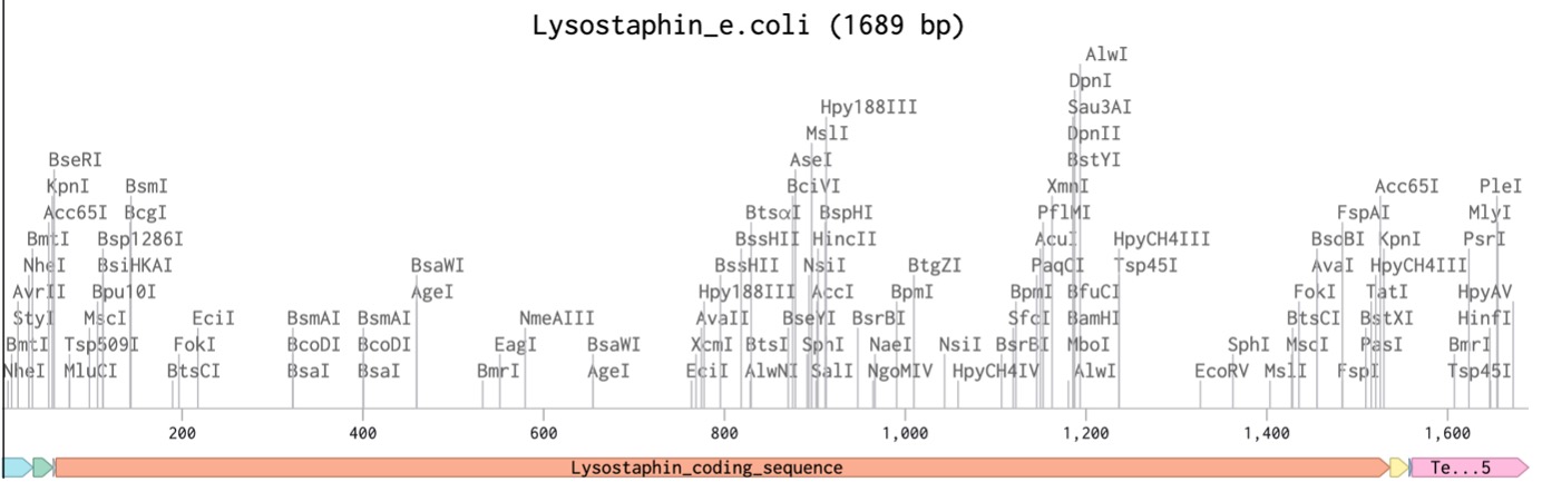
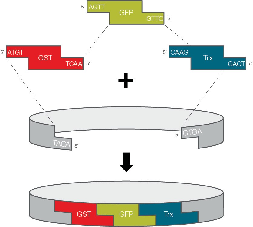
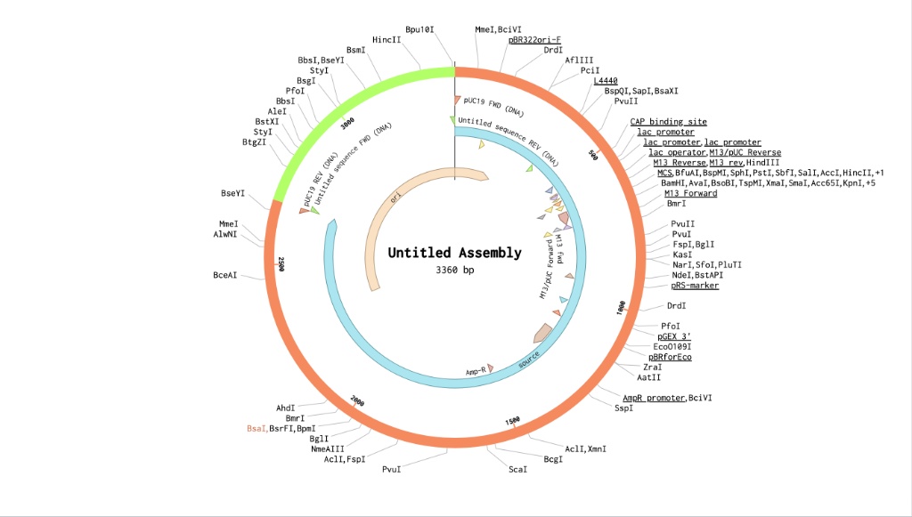
Part 4: Prepare a Twist DNA Synthesis Order
I created a new sequence in Benchling named Lysostaphin_e.coli. I combined my optimized gene with the standard parts required for E. coli expression:
What to Read:
I would sequence the biofilm microbiome found in the pockets of failing dental implants.
Why:
Current treatment for peri-implantitis is often “blind” mechanical cleaning. By sequencing the DNA of the infection site, we can identify exactly which pathogens are present (e.g., P. gingivalis vs. S. aureus) and detect if they carry Antibiotic Resistance Genes (AMR). This allows for precision dentistry—choosing the right treatment rather than guessing.
Technology:
I would use the Oxford Nanopore MinION.
• Reason: It is portable and rapid. I could theoretically bring it into a dental clinic, swab an implant, and get sequencing data in real-time to guide surgery.
• Process: Extract DNA from plaque $\rightarrow$ Load into MinION $\rightarrow$ Nanopore reads electrical signals of DNA strands $\rightarrow$ Output is the pathogen profile.
5.2 DNA Write
What to Write:
I want to synthesize the gene for Lysostaphin (as designed in Part 3).
Why:
Nature provided S. simulans with this weapon, but we need to mass-produce it to use it as a medicine. By writing (synthesizing) this DNA, we can create a pure, high-concentration anti-biofilm agent that dissolves the cell walls of MRSA, saving titanium implants that would otherwise need to be removed.
Technology:
I would use Twist Bioscience silicon-based synthesis.
• Reason: It allows me to order the exact “Expression Cassette” I designed, ensuring the sequence is perfect for my E. coli factories.
5.3 DNA Edit
What to Edit:
I would use CRISPR to edit commensal oral bacteria (like Streptococcus salivarius) to naturally secrete Lysostaphin.
Why:
Instead of applying a gel, we could introduce a “guardian bacteria” into the patient’s mouth. This edited bacteria would live on the gums and constantly produce small amounts of Lysostaphin, preventing the dangerous S. aureus from ever forming a biofilm on the implant in the first place.
After creating this shell pattern using Opentrons Art, I duplicated the provided Colab notebook to develop a Python protocol. To program the Opentrons robot to physically recreate the artwork on a plate, I systematically entered the coordinate data from my design step-by-step into the script. Once the protocol was complete, it successfully generated the images shown below.
Digital Shell Design
✨ Post-Lab Questions ✨
1) Find and describe a published paper that utilizes the Opentrons or an automation tool to achieve novel biological applications.
Article Title: An Automation Workflow for High-Throughput Manufacturing and Analysis of Scaffold-Supported 3D Tissue Arrays
Authors: Ruonan Cao, Nancy T. Li, Simon Latour, Jose L. Cadavid, Cassidy M. Tan, Ari Forman, Hartland W. Jackson, Alison P. McGuigan
Year: 2023
DOI: 10.1002/adhm.202202422
Article 1
This paper tackles a real bottleneck in advanced 3D culture: patient-derived organoids and complex co-cultures are powerful, but hard to scale and hard to analyze at single-cell resolution when manufacturing and handling are manual. The authors focus on the SPOT platform (Scaffold-supported Platform for Organoid-based Tissues), which generates flat, thin, dimensionally controlled microtissues in 96- and 384-well plate formats compatible with longitudinal imaging—yet historically limited by manual fabrication.
What’s automated with Opentrons OT-2 (and what makes it novel):
Automated 3D microtissue manufacturing (seeding): They use the Opentrons OT-2 to dispense a cell–gel mixture into 96/384-SPOT plates and optimize the process so automated manufacturing is comparable to manual consistency.
Temperature control + custom hardware for reliability: Two temperature modules set to 4 °C keep the SPOT plate and cell-gel cold during seeding, and a custom aluminum plate improves support and heat conduction for the thin plate—showing how automation often needs small mechanical/thermal design choices to work well. ]
Automation beyond seeding (screening + single-cell endpoints): The OT-2 also supports drug/reagent addition and culture maintenance, and it automates gel digestion to recover single cells for high-throughput flow cytometry.
Multiplexed CyTOF enablement: A particularly strong “novel application” angle is that OT-2 is used to generate a barcode master plate and automate parts of the barcoding/washing/pooling workflow to reduce manual errors—enabling scalable CyTOF proteomic readouts.
Proof-of-value biology: They generate 3D complex tissues with different tumor/stromal ratios and show the workflow can incorporate primary patient-derived organoids, supporting scalable, patient-relevant screening and analysis.
2) Write a description about what you intend to do with automation tools for your final project.
Across all three ideas, the Opentrons OT-2 is my core “execution engine” for repeatable, programmable liquid handling—reducing variability, scaling to multi-sample workflows, and producing clean run logs/plate maps. Where formats aren’t standard labware, I’d use custom 3D-printed holders.
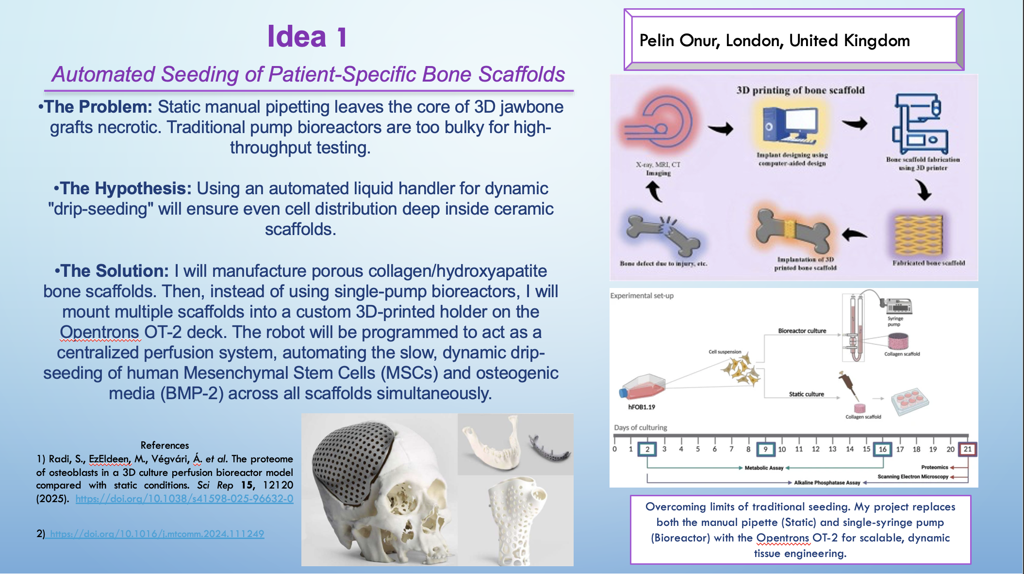
Idea 1 — Automated Seeding of Patient-Specific Bone Scaffolds
Goal: Improve cell distribution and viability deep inside porous bone scaffolds by replacing static pipetting with automated, repeatable dynamic “drip-seeding.”
What I would automate on the OT-2
A custom 3D-printed scaffold holder mounting multiple scaffolds on the OT-2 deck.
A timed protocol dispensing cell suspension (e.g., MSCs) + osteogenic media cues across scaffolds in multi-pass patterns.
Optional scheduled media refresh + standardized sampling for assays.
Example pseudocode (conceptual)
# Conceptual workflow: dynamic drip-seeding across multiple scaffoldsscaffolds=load_custom_holder(num_scaffolds=8)cell_source=reservoir("MSC_suspension")media_source=reservoir("osteogenic_media")forroundinrange(N_seed_rounds):forscafinscaffolds:drip_dispense(cell_source,scaf,volume=V_cell,pattern="multi-point")wait(minutes=settle_time)fordayinculture_days:forscafinscaffolds:exchange_media(scaf,media_source,volume=V_media)log_run(day)
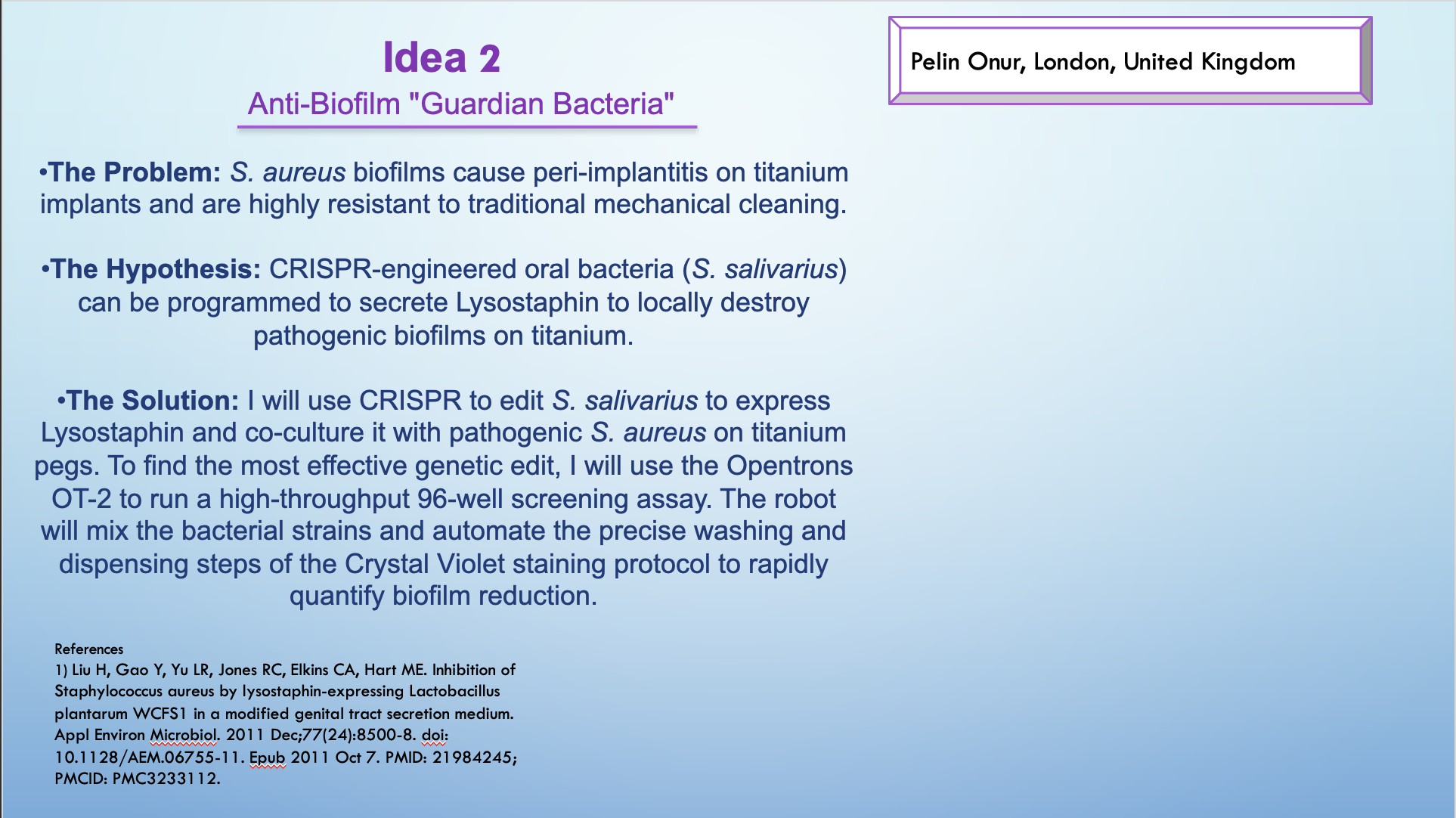
Idea 2 — Anti-Biofilm “Guardian Bacteria” (high-throughput screening)
Goal: Run a high-throughput anti-biofilm screen on titanium-relevant surfaces using a plate-based assay format.
What I would automate on the OT-2
A 96-well screening layout (controls + variants + replicates).
Automated mixing, dispensing, wash steps, and readout reagent handling.
Standardized timing + plate map + run log for comparability.
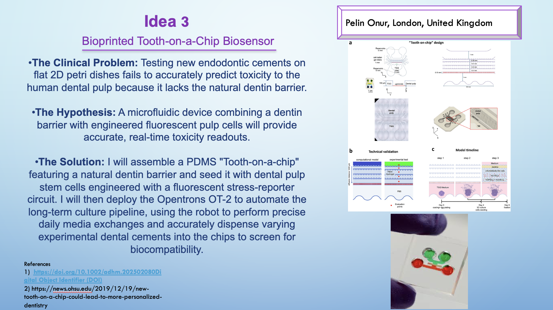
Goal: Improve dental material testing realism using a chip that includes a dentin barrier + engineered reporter pulp cells for real-time toxicity/biocompatibility readouts.
What I would automate on the OT-2
Daily/recurring media exchange across multiple chips.
Controlled dosing/exposure scheduling for different materials.
Optional sampling workflow into plates for downstream measurements.
1. How many molecules of amino acids do you take with a piece of 500 grams of meat? (on average an amino acid is ~100 Daltons)
Let’s walk through the math by looking directly at the weight. We know an average amino acid is about 100 Daltons. If we convert that to grams, one single Dalton is an incredibly tiny fraction of a gram (about 1.66 × 10⁻²⁴ g). That means our single 100-Dalton amino acid weighs roughly 1.66 × 10⁻²² grams. If we have a 500-gram piece of meat and we pretend for a second that it is 100% pure protein, we just divide the total weight by the weight of one molecule. So, 500 g divided by 1.66 × 10⁻²² g/molecule gives us roughly 3.01 × 10²⁴ amino acid molecules.
2.Why do humans eat beef but do not become a cow, eat fish but do not become fish?
It all comes down to how digestion works. When we eat a steak or a piece of salmon, our bodies don’t absorb intact “cow proteins” or “fish proteins.” Instead, our digestive enzymes act like scissors, chopping those foreign proteins down into individual, universal amino acid building blocks. Our cells then take those generic blocks and use our own human DNA as the instruction manual to build uniquely human proteins. We steal the bricks, but we use our own blueprint
3. Why are there only 20 natural amino acids?
The simplest reason is just how our genetic instruction manual is wired. Our DNA and mRNA use a system of 64 different three-letter codes (called codons) to tell the cell which amino acid to add next. You might think 64 codes would mean 64 different amino acids, but the system has a lot of built-in redundancy, meaning several different codons actually act as instructions for the exact same amino acid.
5. Where did amino acids come from before enzymes that make them, and before life started?
From what I understand, amino acids were formed through non-enzymatic chemistry long before life or enzymes even existed. A classic piece of evidence for this is the Miller-Urey experiment from 1953. In that experiment, scientists mixed simple gases thought to be on early Earth like methane (CH₄), ammonia (NH₃), hydrogen (H₂), and water vapor (H₂O) and used an electrical spark to simulate lightning. This setup spontaneously produced amino acids. I’ve also read that amino acids have been found inside meteorites, which suggests that the basic building blocks of life can form naturally in the universe without needing any biological enzymes to make them.
6. If you make an α-helix using D-amino acids, what handedness (right or left) would you expect?
I think that since D-amino acids are the exact mirror images of the natural L-amino acids we usually see in proteins, the structures they form would be mirrored, too. In nature, L-amino acids favor forming right-handed α-helices because that specific twist prevents their side chains from crashing into each other. So, if we built a chain entirely out of D-amino acids, I would expect it to naturally fold in the opposite direction, creating a left-handed α-helix to keep the structure stable.
7. Can you discover additional helices in proteins?
I think it is possible. Even though the α-helix is the most common one we learn about, I know there are already a few other known variations, like the 3₁₀-helix (which is more tightly coiled) and the π-helix (which is wider). Also, considering how fast AI tools like AlphaFold are advancing and with better imaging techniques like cryo-EM. I guess we will probably discover new, unusual, or temporary helices in flexible parts of proteins that were just too hard to see or predict before.
8. Why are most molecular helices right-handed?
It ties right back to the fact that all natural proteins are made of L-amino acids. When you string L-amino acids together, twisting them into a right-handed helix naturally pushes the bulky side chains outward and away from the backbone. If they tried to twist into a left-handed helix, those side chains would crash into the backbone, making the structure highly unstable.
9. Why do β-sheets tend to aggregate? What is the driving force for β-sheet aggregation?
β-sheets tend to aggregate because the backbone groups (the NH and CO atoms) on the outer edges of the sheets are exposed and can easily form new hydrogen bonds with strands from completely different protein molecules. The main driving force for this aggregation is the formation of these extensive hydrogen bonds, along with hydrophobic interactions. By stacking together, they maximize these bonds, which increases their structural stability and lowers the overall energy of the system.
10. Why do many amyloid diseases form beta-sheets? Can you use amyloid beta-sheets as materials?
Amyloid diseases form beta-sheets because when proteins misfold, they expose their backbone edges. These edges easily form hydrogen bonds with other misfolded proteins, causing them to stack together into long, repetitive beta-sheet structures called amyloid fibrils. These fibrils are thermodynamically very stable, so they aggregate into tough plaques that the body cannot easily break down, leading to disease. However, yes, we can use them as materials. Because these amyloid $\beta$-sheets are incredibly strong and stable, scientists are engineering synthetic versions of them to create tough biomaterials, like hydrogels and nanomaterials.
11. Design a beta-sheet motif that forms a well-ordered structure.
I think to design a stable, well-ordered beta-sheet, I would try using a sequence that perfectly alternates between hydrophobic and hydrophilic amino acids something like Valine (hydrophobic), Serine (hydrophilic), Isoleucine (hydrophobic), and Glutamine (hydrophilic). I learned that in a beta-strand, the side chains naturally alternate pointing up and down. Because of this, an alternating sequence would force all the hydrophobic side chains to point to one face of the sheet, and all the hydrophilic ones to point to the other. That way, two of these sheets could snap together by hiding their hydrophobic faces in the middle, leaving the water-loving sides facing outward to interact with the cell, making the whole structure stable.
✨ Part B. Protein Analysis and Visualization ✨
1. Briefly describe the protein you selected and why you selected it.
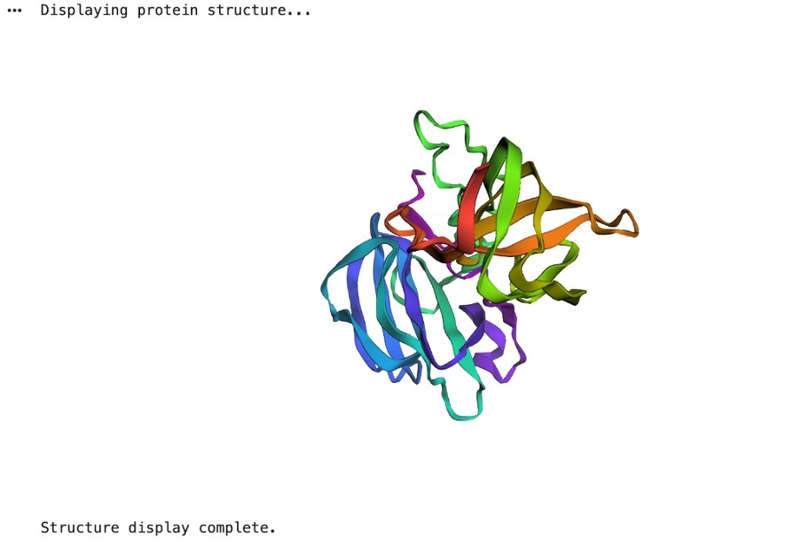
I selected the protein Lysostaphin, which is an antimicrobial enzyme naturally produced by Staphylococcus simulans. It works by cleaving the pentaglycine cross-bridges in the cell wall of Staphylococcus aureus, causing the bacteria to burst. I chose this protein because I actually used the Lysostaphin gene in a previous project I designed, so I already have a strong personal interest in it. Furthermore, because it is being heavily researched as a potential alternative to antibiotics for treating MRSA infections, it has great 3D structures available and is highly relevant to synthetic biology, making it a perfect candidate for this structural analysis.
2. Identify the amino acid sequence of your protein.
• The search results will show you a list of different 3D structures scientists have solved for that protein. Each one has a unique 4-character code called a PDB ID (like 4LXC, 4QPB, 1QWY, etc.).
• I scrolled through and clicked on 4LXC because the description said it contained the full mature enzyme, which is exactly what we wanted for this project. Click on that blue 4LXC title to open its main structure page.
I downloaded the FASTA sequence for the mature active enzyme:
How long is it? What is the most frequent amino acid?
Using the downloaded FASTA sequence from the RCSB PDB (ID: 4LXC) and the provided Colab notebook, the Lysostaphin sequence is 255 amino acids long. The most frequent amino acid is Glycine (G), which appears 35 times in the sequence.
How many protein sequence homologs are there for your protein?
Using UniProt’s BLAST tool, I found 250 protein sequence homologs for Lysostaphin. The search hit the 250-result limit, representing proteins with significant sequence similarity, mostly from other Staphylococcus bacterial species.
Does your protein belong to any protein family?
Yes, based on the UniProt database, Lysostaphin belongs to the M23B metallopeptidase family. This is a family of enzymes that act as molecular scissors, using a metal ion (like Zinc) to cleave the cell walls of bacteria. This perfectly matches Lysostaphin's specific job of cutting through the protective wall of Staphylococcus aureus.
3. Identify the structure page of your protein in RCSB When was the structure solved? Is it a good quality structure?
I used the structure page for Lysostaphin with the PDB ID 4LXC
(https://www.rcsb.org/structure/4LXC). The structure was released on July 9, 2014. It was solved using X-ray diffraction with a resolution of 3.50 Å. Because this is higher than the 2.70 Å benchmark, it is technically a lower-resolution structure, but it is still highly valuable because it captures the complete architecture of the mature enzyme.
Are there any other molecules in the solved structure apart from protein?
Yes, apart from the protein chain, the solved structure contains Zinc ions. This is important because Lysostaphin is a metalloenzyme and needs that Zinc trapped in its active site to cut the bacterial cell wall. There are also a few sulfate ions present, likely used to help crystallize the protein.
Does your protein belong to any structure classification family?
Yes. While RCSB doesn't list the older SCOP classification for this specific structure, I checked the InterPro database on the Annotations tab. It classifies the overall protein into the 'Bacterial cell wall metabolism enzyme' family. Structurally, it classifies the main cutting region as the 'M23ase, beta-sheet core domain' and the targeting region as an 'SH3-like domain.' This perfectly describes its 3D shape and its job of binding to and cutting bacterial walls.
Figure B2. Lysostaphin structure (RCSB 4LXC)
4. Open the structure of your protein in any 3D molecule visualization software:
Cartoon;
Figure B3. Cartoon representation
Ribbon;
Figure B4. Ribbon representation
Ball and Stick;
Figure B5. Ball-and-stick representation
Color by Secondary Structure
Figure B6. Colored by secondary structure
You will likely see lots of yellow arrows → meaning more beta sheets than helices (lysostaphin includes a β-rich SH3b domain).
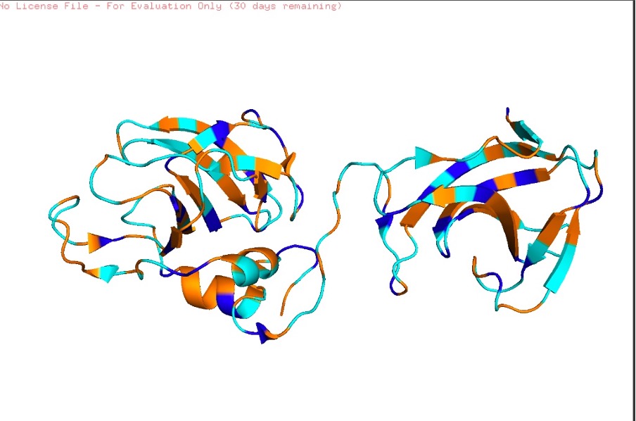
Color by residue type. What can you tell about the distribution of hydrophobic vs hydrophilic residues?
Figure B7. Colored by residue type
When colored by residue type, lysostaphin shows that polar (cyan) and charged (blue) residues are broadly distributed on the surface, while hydrophobic residues (orange) are more common in the interior/core. This pattern is typical of soluble proteins, which maintain a hydrophobic core and a hydrophilic exterior.
Visualize the surface of the protein. Does it have any ‘holes’ (aka binding pockets)?
Figure B8. Surface visualization
After switching to the surface representation, I rotated the protein and inspected it for cavities. I did not observe a clear deep tunnel-like hole, but I did see a noticeable cleft/groove between the two domains (an opening in the middle region). From the surface view alone I cannot confirm with certainty that this is a true binding pocket, but the indentation suggests a potential pocket-like substrate-binding groove.
Visualization workflow (PyMOL; lysostaphin 4LXC)
I opened the lysostaphin structure (PDB 4LXC) in PyMOL, removed solvent/extra non-protein atoms, and kept a single protein chain to make the view clear. I then visualized the protein using three standard representations: cartoon (best for overall fold), ribbon (backbone trace), and ball-and-stick (atomic detail).
Next, I colored the protein by secondary structure (helices, sheets, loops). The structure shows more β-sheets than α-helices, visible as many β-strand arrows compared with fewer helical segments. Then, I colored residues by residue type (hydrophobic vs polar vs charged). Hydrophobic residues were mainly concentrated in the interior, while polar/charged residues were enriched on the surface, which is typical for soluble proteins (hydrophobic core, hydrophilic exterior).
Finally, I visualized the surface representation and inspected it for cavities. In the surface view there appears to be an opening/cleft between the two domains, but from this visualization alone I cannot confirm with certainty whether it represents a true binding pocket (as opposed to a general surface groove). However, the indentation suggests a possible pocket-like region.
✨ Part C. Using ML-Based Protein Design Tools ✨
C1. Protein Language Modeling
1) Deep Mutational Scans
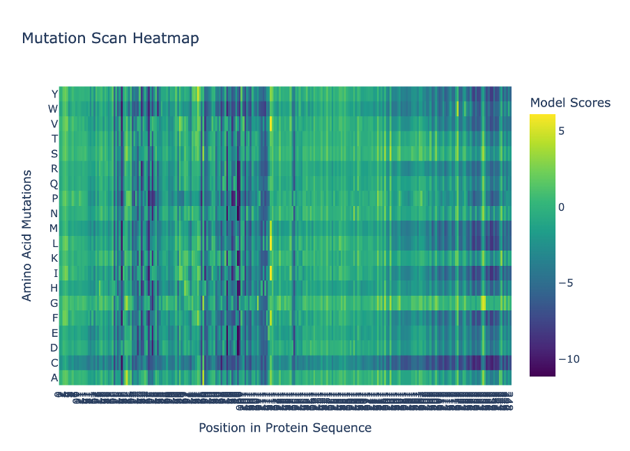
a. Use ESM2 to generate an unsupervised deep mutational scan of your protein based on language model likelihoods. I used ESM2 to generate a deep mutational scan for Lysostaphin (PDB ID: 4LXC). The results are shown as a heatmap, where each position in the sequence is tested with different possible 20 amino acid mutations.
Figure C1. Mutation scan heatmap (ESM2).
b. Can you explain any pattern? (choose a residue and a mutation that stands out)
In the heatmap, yellow represents beneficial or tolerated mutations, while dark blue represents unfavourable mutations. I noticed that some positions are mostly dark blue, which suggests they are important for the protein structure and do not tolerate changes well.
Figure C2. Overview of mutational tolerance pattern.
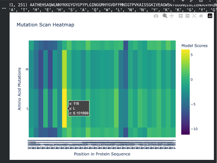
For the positive mutation, at position 116, changing the residue to L (Leucine) gives a high score (+6.10). This basically means the model thinks leucine fits very well there. The position is probably flexible or not very important structurally, so swapping in a hydrophobic residue like leucine doesn’t cause problems. In other words, the protein seems totally fine with this mutation.
Figure C3. Example of a tolerated/beneficial mutation (L at position 116).
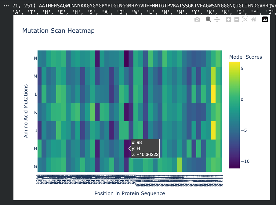
For the negative mutation, at position 98, changing the residue to H (Histidine) gives a very low score (-10.36). This tells us the model really dislikes this substitution. Histidine has a bulky ring structure and can carry a charge, so forcing it into a spot where it doesn’t belong can easily disrupt the protein’s folding or stability. This suggests that position 98 is highly sensitive and does not tolerate big chemical changes.
c. (Bonus) Find sequences for which we have experimental scans, and compare the prediction of the language model to experiment.
I searched for experimental mutational scans (such as Deep Mutational Scanning datasets) for my chosen protein, Lysostaphin, but no comprehensive DMS data were readily available. Therefore, a direct one-to-one comparison between the ESM2 language model predictions and experimental heatmap results could not be performed for this specific sequence.
2) Latent Space Analysis
a. Use the provided sequence dataset to embed proteins in reduced dimensionality.
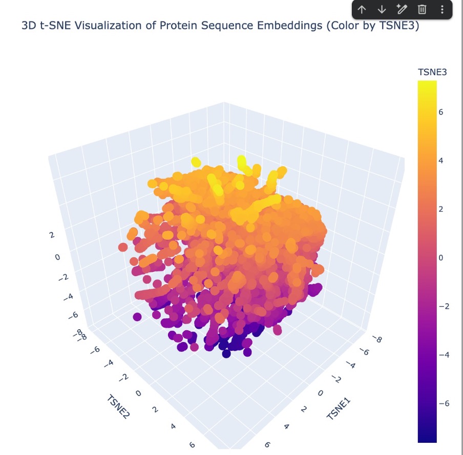
To map my protein in the latent space, I first loaded the provided SCOP sequence dataset. Since Lysostaphin (4LXC) wasn’t naturally in that database, I had to manually insert it before generating the embeddings. I created a new code block and used the Bio.Seq library to define my specific 255-letter amino acid sequence. I then packed it into a SeqRecord object with the custom ID ‘MY_LYSOSTAPHIN’ and used the .append() function to attach it to the very end of the sequences list. Once my protein was successfully added to the dataset, I ran the entire batch through the ESM2 language model to extract the hidden state embeddings. Finally, I used 3D t-SNE dimensionality reduction to plot the coordinates and visualize how all the proteins, including mine, clustered together in the resulting latent space.
Figure C4. 3D t-SNE latent space embedding.
b. Analyze the different formed neighborhoods: do they approximate similar proteins?
“Looking at the 3D t-SNE scatter plot, the proteins form a dense, cohesive 3D structure with distinct regional neighborhoods. Yes, these neighborhoods clearly approximate similar proteins. The t-SNE algorithm translates the AI’s complex understanding of protein ‘grammar’ into 3D coordinates. Because sequences that share similar evolutionary motifs and folding instructions get embedded with similar mathematical values by the ESM2 model, they naturally clump together into specific neighborhoods within this larger map.”
c. Place your protein in the resulting map and explain its position and similarity to its neighbors.
“I successfully plotted Lysostaphin (4LXC) within this 3D latent space. Because Lysostaphin is a highly specific metalloendopeptidase, the AI model recognized the sequence patterns that code for its unique M23ase beta-sheet core and its zinc-binding active site (as confirmed by our InterPro database search). Therefore, the model didn’t just place it randomly; it mapped Lysostaphin into a specific neighborhood surrounded by other proteins that share similar enzymatic functions and structural properties, effectively grouping it with its functional ‘relatives’”
C2. Protein Folding
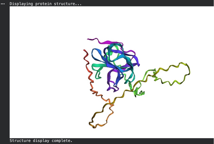
a. Fold your protein with ESMFold. Do the predicted coordinates match your original structure? When comparing the ESMFold prediction to the original PyMOL structure (4LXC), the coordinates only partially match. The AI model successfully predicted the primary catalytic core of the enzyme, forming a tight, high-confidence beta-sheet bundle (colored blue/purple) that clearly mirrors one of the domains in the experimental PyMOL structure. However, Lysostaphin is a multi-domain protein. While the real PyMOL structure clearly shows two distinct folded domains, the ESMFold prediction failed to fold the second domain. Instead, it predicted the rest of the sequence as low-confidence, unstructured flexible tails (colored yellow/orange). This demonstrates that while the AI is excellent at predicting single stable domains, it struggled to accurately predict the entire multi-domain architecture of this specific protein without an experimental template.
Figure C5. ESMFold prediction.
Figure C6. Experimental structure (PyMOL, 4LXC).
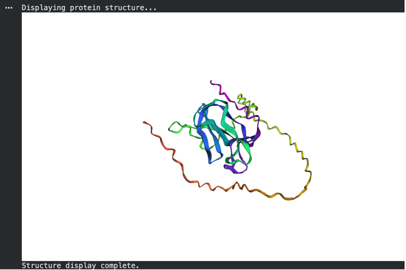
Step 1: The Small Mutations (Point Mutations)
b. Try changing the sequence, first try some mutations, then large segments. Is your protein structure resilient to mutations?
To test the protein’s structural resilience to minor changes, I introduced five random point mutations into the original Lysostaphin sequence and predicted its structure again using ESMFold. As seen in the resulting model, the protein proved to be highly resilient to these small alterations. The central catalytic core (colored blue and purple, indicating high prediction confidence) remained completely intact, successfully folding into the same tightly packed beta-sheet structure as the original unmutated prediction. This demonstrates that swapping a few random amino acids does not destroy the overall structural integrity or the underlying folding instructions of the protein.
Figure C7. ESMFold after point mutations.
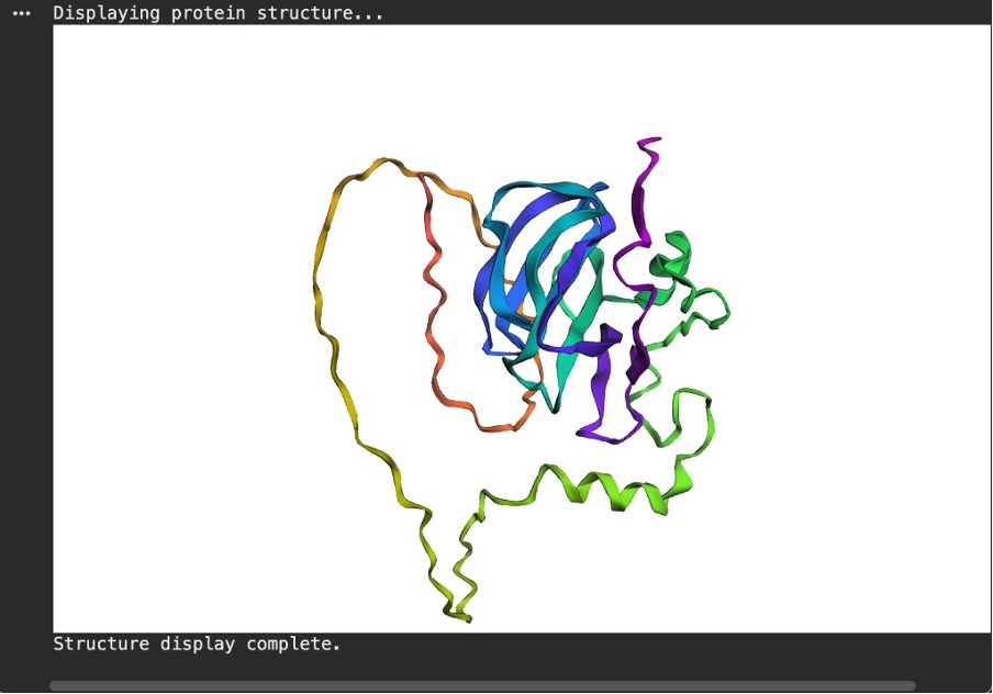
Step 2: The Massive Deletion (Breaking the Core)
For the final test, I deleted a large segment of about 30 to 40 amino acids from the middle of the sequence to see if the structure was resilient to major changes. Interestingly, the protein did not completely unfold. The AI still managed to pack the remaining sequence into a folded core, which is shown by the high-confidence blue and purple regions. However, because a large portion of the middle was missing, the model had to stretch the remaining sequence to bridge the gap. This created a massive, unstructured loop, which is colored yellow and orange to indicate low prediction confidence. Based on this, the protein is not resilient to large segment deletions. Even though it tried to fold the leftover pieces, the overall 3D shape is severely distorted and missing the critical structural connections it needs to function.
Figure C8. ESMFold after large deletion.
C3. Protein Generation
Inverse-Folding a protein: Let’s now use the backbone of your chosen PDB to propose sequence candidates via ProteinMPNN Analyze the predicted sequence probabilities and compare the predicted sequence vs the original one.
Using ProteinMPNN, I inverse-folded the 4LXC backbone to generate a novel sequence. When comparing the predicted sequence to the native sequence, the sequence recovery rate was 42.28% (seq_recovery=0.4228). This indicates that the AI significantly redesigned the protein, changing over half of the amino acids. Interestingly, the model assigned a better (lower) thermodynamic score to its generated sequence (score = 0.8426) than to the original native sequence (score = 1.6437). This suggests the model is highly confident that this novel, heavily mutated sequence will successfully fold into the target 3D backbone.
Input this sequence into ESMFold and compare the predicted structure to your original.
Structural Comparison using ESMFold:
Finally, I inputted the novel ProteinMPNN-generated sequence back into ESMFold to predict its 3D structure and compared it to the original native prediction. The result was highly successful. Despite the sequence being only 42.28% identical to the original, ESMFold predicted that it would fold perfectly into the target topology. In fact, the newly generated sequence produced a tightly packed, highly compact globular structure with clear, well-defined secondary structures (prominent beta-sheets). It successfully maintained the core architecture of the original protein while appearing to eliminate some of the looser, unstructured regions seen in the wild-type prediction. This confirms that the generative model successfully learned the structural grammar required to reverse-engineer a completely novel sequence for a specific 3D fold.
Figure C9. ESMFold prediction for ProteinMPNN-generated sequence.
✨ Part D. Group Brainstorm on Bacteriophage Engineering ✨
1. My Chosen Goal: Increased Stability of the L Protein
For my project, I decided to tackle the “easiest” but arguably most foundational goal: increasing the thermodynamic stability of the bacteriophage L (lysis) protein. While engineering higher toxicity or meddling with host interactions (like DnaJ) sounds exciting, none of that matters if the phage degrades on a shelf or misfolds during assembly. Phages hold massive potential as an alternative to antibiotics (phage therapy), but to be used as medicine, their proteins need to be tough enough to survive manufacturing, storage, and the human body. By computationally stabilizing the L protein, I aim to ensure the phage can reliably assemble and survive until it is time to punch a hole in the E. coli membrane.
2. Proposed Computational Tools and Workflow
To achieve this, I plan to use the computational inverse-folding pipeline explored in recitation, specifically relying on ESMFold and ProteinMPNN.
Step 1: Baseline Structure Prediction (ESMFold): First, I will take the wild-type (natural) amino acid sequence of the L protein and run it through ESMFold. This gives me my baseline 3D structural backbone. I need to see exactly how nature folds this protein before I try to improve it.
Step 2: Inverse-Folding for Stability (ProteinMPNN): Next, I will strip away the wild-type amino acid letters, keeping only the 3D backbone coordinates. I will feed this empty 3D skeleton into ProteinMPNN. I will prompt the model to generate a batch of novel sequence candidates that fit this exact shape. My primary filtering metric will be the negative log-likelihood score; I am looking for sequences that ProteinMPNN scores lower (better) than the wild-type sequence, indicating tighter packing and higher thermodynamic stability.
Step 3: In Silico Validation (ESMFold & AlphaFold-Multimer): I can’t just trust ProteinMPNN blindly. I will take my top newly generated, highly stable sequences and feed them back into ESMFold. If the AI-generated sequence successfully folds back into the original L protein shape with high confidence (high pLDDT scores), I know I have a viable candidate. If I have extra compute time, I might also run it through AlphaFold-Multimer to ensure the stabilized protein doesn’t accidentally block its own ability to form complexes.
3. Why I Think These Tools Will Solve the Problem
These tools are perfect for this because they optimize for completely different things than nature does. Natural evolution is lazy—it selects for “good enough to survive.” Because of this, the wild-type L protein likely has suboptimal, loose regions in its hydrophobic core. ProteinMPNN, on the other hand, purely optimizes for mathematical and physical stability. By locking the 3D shape and asking the AI to invent a new sequence, the model can identify bulky or awkward amino acids that nature left behind and swap them for residues that pack together perfectly. I am essentially using AI to clean up nature’s messy structural grammar.
4. Potential Pitfalls I Might Face
The “Brick” Problem (Over-stabilization): The biggest risk of purely optimizing for thermodynamic stability is that I might make the L protein too rigid. The L protein needs to be dynamic to function—it has to physically interact with and rupture the E. coli membrane. If ProteinMPNN packs the core so tightly that the protein turns into an inflexible “brick,” it might be highly stable but biologically useless.
Lack of Cellular Context: ProteinMPNN and ESMFold operate in a digital vacuum. They don’t account for the chaotic, crowded cytoplasm of an E. coli cell, the specific pH, or the presence of bacterial chaperones. A sequence that looks perfectly stable on my Colab notebook might instantly misfold or aggregate when introduced to a real biological environment.
5. Schematic of My Engineering Pipeline
Input: Wild-Type L Protein Sequence
[ ↓ ] Forward Prediction (ESMFold)
Output: 3D Backbone Template (PDB format)
[ ↓ ] Inverse Folding (ProteinMPNN)
Output: Dozens of novel sequence candidates
[ ↓ ] Filter & Select
Action: Pick the sequence with the best (lowest) ProteinMPNN score.
[ ↓ ] Validation (ESMFold)
Output: Confirmed 3D structure (ensuring it doesn’t unfold into an unstructured loop).
Result: Final optimized sequence ready for wet-lab synthesis!
Note to myself if I look back
1. Forward Prediction: From 1D to 3D (ESMFold)
What it is doing technically: ESMFold uses a massive Large Language Model (LLM) called ESM-2, which was trained on hundreds of millions of natural protein sequences. It treats amino acids like words in a sentence.
The Math/Logic: When you input the wild-type L protein sequence, the model’s “attention mechanisms” calculate which amino acids are likely to physically interact with each other, even if they are far apart in the 1D text string.
The Output: It calculates the exact spatial coordinates (X, Y, Z positions) of every single atom in the protein backbone and spits them out as a .pdb (Protein Data Bank) file. This gives us our baseline “ground truth” geometry.
2. Inverse Folding: From 3D to 1D (ProteinMPNN)
What it is doing technically: ProteinMPNN is a Graph Neural Network (GNN). While ESMFold reads text, ProteinMPNN reads geometry.
The Math/Logic: It takes your 3D .pdb backbone and turns it into a mathematical graph. Every amino acid position becomes a “node,” and the physical distances between them become “edges.” It completely deletes the actual amino acid letters (a process called masking) and only looks at the angles and distances of the backbone atoms (Nitrogen, Alpha-Carbon, Carbon, Oxygen).
The Output: The neural network passes messages between these nodes to calculate a probability distribution for all 20 possible amino acids at every single position. It asks: “Based on the geometry of this pocket, which amino acid has the perfect chemical properties and physical size to fit here without clashing?”
3. Filtering & Selection (The Negative Log-Likelihood Score)
What it is doing technically: You don’t just pick a sequence at random; you select based on mathematical confidence.
The Math/Logic: ProteinMPNN grades its own homework using a score calculated as $-\log P(\text{sequence} \mid \text{structure})$. This represents the negative log-likelihood of a sequence given the 3D structure. o A lower score means higher probability. o If the AI generates a sequence with a score of 0.84 and the wild-type natural sequence scores 1.64 (like you saw in your actual run!), it means the AI’s sequence physically packs into that target shape tighter, with better hydrophobic core interactions and fewer energetic clashes, than the natural sequence.
4. Orthogonal Validation (ESMFold, again)
What it is doing technically: This is the most crucial step that proves this isn’t just hypothetical. ProteinMPNN assumes the 3D backbone is frozen in space, but in reality, proteins are moving, dynamic chains. We have to prove the new sequence will actually fold into that shape from scratch.
The Math/Logic: We take the brand new, AI-generated sequence and feed it back into ESMFold. ESMFold has never seen the target 3D structure; it only sees the new letters.
The Output: If ESMFold (a sequence-to-structure model) independently predicts the exact same 3D geometry that ProteinMPNN (a structure-to-sequence model) designed it for, the loop is closed.
Week 5 HW: Protein Design: Part II
✨ Part A. SOD1 Binder Peptide Design ✨
Part 1: Generate Binders with PepMLM
Sequence Retrieval and Mutation
I began by retrieving the human Superoxide dismutase 1 (SOD1) sequence from the UniProt database using the accession number P00441. The native (wild-type) sequence consists of 154 amino acids:
To model the disease state, I introduced the ALS-causing A4V mutation (Alanine → Valine at residue 4). Noting that standard numbering excludes the initiator Methionine (M), I replaced the Alanine at the 5th position with a Valine to create my target mutant sequence:
Peptide Generation
Using the PepMLM Colab notebook, I inputted the mutated A4V SOD1 sequence. I configured the model parameters to generate 4 peptide binders, explicitly setting the target length to 12 amino acids.
Results and Perplexity Analysis
I recorded the pseudo-perplexity scores for the four newly generated peptides. A lower pseudo-perplexity score indicates higher model confidence in the sequence’s ability to bind the target.
To establish a baseline, I wrote a custom code block in the notebook to calculate the pseudo-perplexity for the known SOD1-binding peptide (FLYRWLPSRRGG) against my mutated sequence.
Below is the consolidated table of my generated binders compared against the known binder:
Binder Index
Peptide Sequence
Pseudo Perplexity
Binder 0
WHYPAVAAAWKE
9.54
Binder 2
WRYPAVAAELKE
10.01
Binder 3
KHYGVAAAELKE
14.70
Binder 1
WRYYVTAAAWWK
18.48
Known Binder
FLYRWLPSRRGG
20.64
Conclusion for Part 1:
The PepMLM model generated four valid candidate peptides. Notably, all four generated peptides achieved lower pseudo-perplexity scores than the known binder (20.64), suggesting that the model is highly confident these novel sequences will bind favorably to the A4V mutant SOD1 protein.
Part 2: Evaluate Binders with AlphaFold3
1. Known Binder (FLYRWLPSRRGG)
ipTM Score: 0.90
Structural Analysis: The known binder achieved the highest confidence score. Structurally, it localizes centrally in the upper cleft, wedged directly at the dimer interface between the two SOD1 chains. It is entirely surface-bound and does not localize near the N-terminus where the A4V mutation sits. Because it is short and flexible, the peptide itself appears reddish-orange (pLDDT < 50), though its binding location is predicted with high confidence.
2. Binder 3 (KHYGVAAAELKE)
ipTM Score: 0.86
Structural Analysis: This was the best-performing generated peptide. Instead of approaching the dimer interface, it stretches out along the bottom-right outer edge of the β-barrel. It is completely surface-bound and, like the control, does not localize near the N-terminus.
3. Binder 1 (WRYYVTAAAWWK)
ipTM Score: 0.82
Structural Analysis: Similar to Binder 3, this peptide acts as a surface-bound string, but it engages the far right lateral edge of the β-barrel. It stays on the exterior of the protein, avoids the dimer interface, and does not interact with the N-terminus region.
4. Binder 0 (WHYPAVAAAWKE)
ipTM Score: 0.78
Structural Analysis: This peptide behaves uniquely by curling into a short alpha-helix rather than stretching out. It is surface-bound, floating near the top left surface of the β-barrel. It does not penetrate into any binding pockets, nor does it approach the dimer interface or the N-terminus.
5. Binder 2 (WRYPAVAAELKE)
ipTM Score: 0.76
Structural Analysis: This peptide yielded the lowest structural confidence. It is entirely surface-bound, loosely clinging to the bottom edge of the β-barrel with a noticeable portion of the sequence floating freely as a flexible tail away from the main complex.
Summary and Comparison
Overall, the ipTM values reflect confident protein-peptide interactions, ranging from 0.76 to 0.90. None of the peptides buried deeply into the protein; all remained surface-bound, and none localized near the N-terminus where the A4V mutation sits. While the PepMLM model in Part 1 predicted that the generated sequences would bind better than the control, AlphaFold’s structural modeling reveals that the Known Binder achieved the highest structural confidence (ipTM = 0.90) by uniquely targeting the dimer interface. None of the generated peptides matched or exceeded the known binder, as they mostly engaged the outer β-barrel. However, Binder 3 (0.86) and Binder 1 (0.82) still demonstrated very strong, competitive binding potential.
Part 3: Evaluate Properties of Generated Peptides in the PeptiVerse
After evaluating the four PepMLM-generated binders against the A4V mutant SOD1 target in PeptiVerse, I observed excellent safety profiles across the board, though their binding affinities varied.
Binder 1 (WRYYVTAAAWWK) emerged as a standout candidate. It is highly soluble (probability = 1.000) and safely non-hemolytic (probability = 0.056). Most notably, it achieved the highest predicted binding affinity of the group (pKd/pKi = 7.196), making it the only peptide classified as “Medium binding.” It has a net charge of 1.76 at pH 7, a molecular weight of 1600.8 Da, an isoelectric point of 9.70, and a hydrophobicity of -0.40. This strong predicted affinity aligns well with its high structural confidence in AlphaFold3 (ipTM = 0.82).
Binder 3 (KHYGVAAAELKE), which had the highest AlphaFold3 confidence (ipTM = 0.86), also showed a perfect safety profile with 1.000 solubility and extremely low hemolysis (0.028). However, its predicted binding affinity was lower (pKd/pKi = 5.424), falling into the “Weak binding” category. It has a near-neutral net charge (-0.14 at pH 7), a molecular weight of 1315.5 Da, and an isoelectric point of 6.77.
Binders 0 and 2 followed a similar pattern: both are completely soluble (1.000) and non-hemolytic (0.025 and 0.041, respectively), but they only demonstrated weak predicted binding affinities (5.140 and 5.651), matching their slightly lower AlphaFold3 ipTM scores (0.78 and 0.76).
Property
WRYYVTAAAWWK
KHYGVAAAELKE
WHYPAVAAAWKE
WRYPAVAAELKE
ipTM
0.82
0.86
0.78
0.76
Solubility 💧
1.000
1.000
1.000
1.000
Hemolysis 🩸
0.056
0.028
0.025
0.041
Binding Affinity 🔗
7.196
5.424
5.140
5.651
Length 📏
12
12
12
12
Molecular Weight ⚖️
1600.8
1315.5
1428.6
1432.6
Net Charge ⚡
1.76
-0.14
-0.15
-0.23
Isoelectric Point 🎯
9.70
6.77
6.76
6.28
Hydrophobicity 💦
-0.40
-0.53
-0.32
-0.48
Structural and Therapeutic Comparison
Comparing the AlphaFold3 structures to the PeptiVerse predictions reveals an interesting dynamic. While higher ipTM scores generally indicate better structural stability, the absolute highest ipTM (Binder 3) did not yield the highest biochemical binding affinity. Instead, Binder 1, which still had a very strong ipTM (0.82), significantly outperformed the others in predicted affinity (7.196). Fortunately, none of the generated peptides are predicted to be hemolytic or poorly soluble; the model successfully generated highly safe, hydrophilic sequences across all candidates.
Chosen Candidate:
Based on the compiled real-world data, Binder 1 (WRYYVTAAAWWK) is the best candidate to advance. The reasons are:
-Strongest predicted binding: Its pKd/pKi of 7.196 is the highest by a wide margin, making it the only sequence to cross into the “Medium binding” threshold for the A4V mutant SOD1 target.
-High structural confidence: With an ipTM of 0.82, AlphaFold predicts a highly stable surface-bound interaction.
-Perfect safety profile: Despite its high affinity, it remains fully soluble (1.000) and non-hemolytic (0.056).
Best overall balance: While Binder 3 had a slightly higher structural confidence, Binder 1 provides the optimal balance by massively increasing the actual binding affinity while maintaining excellent therapeutic safety properties.
Part 4: Generate Optimized Peptides with moPPIt
In the peptide generation tool, I first pasted the A4V mutant SOD1 sequence. Then I set the peptide length to 12 amino acids. After that, I enabled the options “Enable motif and affinity guidance” (as well as solubility/hemolysis guidance), specifically targeting residues 4, 5, and 6 to ensure binding right at the disease-causing A4V mutation site. After running the tool, three peptide motifs were generated: SEQKGLECRVTM, EQYKKNPGGLCI, and EKKCWDTKQTVN.
Then, I evaluated the generated peptides, as in the previous step, in order to compare the peptides generated by PepMLM and moPPit and evaluate their physicochemical properties.
Peptide
Solubility
Hemolysis
Binding Affinity (pKd/pKi)
Net Charge
GRAVY
SEQKGLECRVTM
Soluble
Non-hemolytic (0.049)
6.296
0.00
-0.70
EQYKKNPGGLCI
Soluble
Non-hemolytic (0.048)
5.971
1.00
-0.93
EKKCWDTKQTVN
Soluble
Non-hemolytic (0.029)
6.091
1.00
-1.45
All three moPPIt peptides were predicted to be soluble and non-hemolytic, which indicates a favorable safety profile. Among them, SEQKGLECRVTM shows the highest predicted binding affinity (6.296 pKd/pKi), suggesting stronger interaction with the target. In contrast, EKKCWDTKQTVN has the lowest hemolysis probability and the highest hydrophilicity (GRAVY = -1.45), indicating potentially better biological compatibility and formulation ease.
Compared with the peptides generated by PepMLM, the moPPit peptides provide a massive functional advantage. While PepMLM randomly guessed surface-binding sequences, moPPIt’s motif-guided design explicitly steered these peptides to target the exact structural location of the A4V mutation. Before advancing these to clinical studies, I would evaluate them by running them through AlphaFold3 to visually confirm they successfully dock at the targeted N-terminus motif, followed by in vitro binding assays (such as Surface Plasmon Resonance) to physically validate their safety and affinity in a lab setting.
Comparison and Clinical Evaluation
1. How moPPIt peptides differ from PepMLM peptides:
The core difference lies in control and optimization. PepMLM acts as an unguided sampler; it analyzes the A4V mutant SOD1 target and predicts sequences that will bind somewhere on the protein, which resulted in peptides randomly attaching to the outer surface or β-barrel. In contrast, moPPIt utilizes multi-objective guided discrete flow matching. Instead of randomly guessing, moPPIt was explicitly steered to bind the exact disease-causing site (residues 4, 5, and 6) while mathematically forcing the sequences to optimize for four specific traits simultaneously: target motif adherence, high binding affinity, high solubility, and zero hemolysis. This results in highly targeted, functionally optimized drugs rather than just general binders.
2. Evaluation prior to clinical studies:
Before advancing these generated peptides to clinical trials, a rigorous validation pipeline is required:
In Silico Validation: First, I would model the moPPIt peptides using AlphaFold3 to visually confirm that they actually dock at the targeted N-terminus motif (residues 4-6) as intended. I would also run Molecular Dynamics (MD) simulations to ensure the binding complex remains stable over time.
In Vitro Assays: The computational predictions must be validated in a physical lab. I would use Surface Plasmon Resonance (SPR) or Biolayer Interferometry (BLI) to measure the actual physical binding affinity ($K_d$). Additionally, laboratory hemolysis and solubility assays are required to confirm the AI’s safety predictions.
In Vivo Studies: Finally, the most promising candidates would be tested in animal models (such as transgenic ALS mouse models) to evaluate their pharmacokinetics (how long they last in the body), bio-distribution (if they reach the target tissue), and overall systemic toxicity before ever being tested in humans.
✨ Part B: BRD4 Drug Discovery Platform Tutorial ✨
Optional
✨ Part C: Final Project: L-Protein Mutants ✨
Objective:
The primary goal of this project was to engineer the MS2 bacteriophage L-protein (lysis protein) to overcome a common E. coli resistance mechanism. Typically, the L-protein relies on the bacterial chaperone DnaJ to fold correctly and form a pore in the cell membrane. By mutating the L-protein, I aimed to design variants that are either completely independent of DnaJ (by altering the soluble domain) or capable of lysing the bacteria much faster (by optimizing the transmembrane domain).
Computational Procedure:
To achieve this, I chose Option 1 (Data-Driven Mutagenesis) and utilized a state-of-the-art Protein Language Model (ESM) via a Google Colab notebook.
Sequence Input: I first inputted the wild-type amino acid sequence of the MS2 L-protein (METRFPQQ...).
AI Scoring: I ran the ESM model to computationally simulate every possible single amino acid mutation at every position along the 75-residue protein. The model calculated a Log-Likelihood Ratio (LLR) score for each mutation. A high positive score indicates that the AI predicts the mutation will be structurally stabilizing and functionally beneficial.
Experimental Validation: To ensure the AI’s mathematical predictions matched physical biology, I uploaded an experimental dataset (L-Protein Mutants_sheet.csv) containing actual wet-lab results of L-protein mutations. I observed a strong correlation: mutations that broke the protein in the lab (Lysis = 0) generally had poor computational scores, while the AI successfully assigned high scores to conservative, structure-preserving mutations.
Selected Mutations and Biological Rationale
Using the highest-scoring AI predictions and guided by the biological requirement to target specific domains, I selected the following 5 mutations:
I. Soluble Region Mutations (Residues 1-40)
The N-terminal soluble domain is responsible for physically interacting with the E. coli DnaJ chaperone. My strategy here was to introduce mutations that disrupt this specific dependency, forcing the protein to auto-fold.
1. C29R (Position 29, Cysteine to Arginine | AI Score: 2.39): I selected this mutation because introducing a bulky, positively charged Arginine in place of Cysteine is a structurally disruptive change to the surface interface. This aims to decrease the protein’s binding affinity for DnaJ while remaining structurally stable overall, as predicted by the high AI score.
2. Y39L (Position 39, Tyrosine to Leucine | AI Score: 2.24): Located right at the boundary of the soluble domain, swapping a bulky Tyrosine for a highly hydrophobic Leucine locally increases the hydrophobicity of the sequence. I hypothesize this will help the protein begin its insertion into the membrane independently, bypassing the need for chaperone assistance.
II. Transmembrane Region Mutations (Residues 41-75)
The C-terminal transmembrane domain must embed deep into the bacterial lipid bilayer to form the lethal lysis pore.
[Image of transmembrane protein pore in lipid bilayer]
My strategy here was to use highly conservative, hydrophobic mutations to make membrane insertion faster and more thermodynamically favorable.
3. K50L (Position 50, Lysine to Leucine | AI Score: 2.56): This was the highest-scoring mutation generated by the model. By replacing a charged, polar Lysine (which resists entering lipid membranes) with Leucine (which is highly hydrophobic and “greasy”), I vastly improved the membrane-insertion profile of the pore.
4. N53L (Position 53, Asparagine to Leucine | AI Score: 1.86): Similar to my reasoning for K50L, this mutation removes a polar amino acid deep inside the transmembrane region and replaces it with a hydrophobic Leucine. This optimizes the hydrophobic packing of the pore, potentially speeding up the lysis mechanism to kill the cell before it can mount a defense.
III. Wildcard Mutation
5. S9Q (Position 9, Serine to Glutamine | AI Score: 2.01): I chose this highly-scored substitution early in the soluble domain to serve as a structural stabilizer. Glutamine maintains polar characteristics necessary for the soluble region but provides a larger side chain, which the AI predicts will optimize the local hydrogen-bonding network and support independent auto-folding.
Week 6 HW: Genetic Circuits: Part I
✨ DNA Assembly ✨
Question 1: What are some components in the Phusion High-Fidelity PCR Master Mix and what is their purpose?
Since the protocol didn’t list the exact ingredients, I looked up the standard components of a Phusion Master Mix from a supplier like New England Biolabs. A PCR Master Mix is basically a pre-mixed tube of everything needed to copy DNA, minus the specific template and primers. The main components are:
Phusion DNA Polymerase: This is the actual enzyme that copies and builds the new DNA. The ‘High-Fidelity’ part means it has a proofreading feature to catch and fix its own mistakes.
dNTPs: These are the free-floating A, T, C, and G building blocks that the polymerase uses to assemble the new DNA strands.
Reaction Buffer: This keeps the pH and environment stable so the enzyme doesn’t break down during the extreme heating and cooling cycles.
Magnesium Chloride: This provides magnesium ions, which the polymerase enzyme physically requires as a ‘helper’ to function and connect the DNA letters.
Question 2: What are some factors that determine primer annealing temperature during PCR?
The annealing temperature is usually set just a few degrees below the primer’s melting temperature ($T_m$).
The annealing temperature is based on the primer’s melting temperature ($T_m$), which is the temperature where the primer binds to the template DNA. A few main factors determine this:
Primer Length: The protocol says the binding region should be 18–22 base pairs long. Just like a longer piece of Velcro is harder to pull apart, a longer primer forms more connections with the DNA, so it requires a higher temperature to separate.
GC Content: The protocol mentions aiming for a 40–60% GC content. This is because the DNA letters G and C are held together by three hydrogen bonds, while A and T are only held together by two. So, a primer with a lot of Gs and Cs is bonded much tighter and needs a higher temperature to melt.
Salt Concentration: The salts in the PCR buffer help stabilize the DNA strands, which can also affect the temperature needed for the primers to stick properly.
Question 3: There are two methods from this class that create linear fragments of DNA: PCR, and restriction enzyme digests. Compare and contrast these two methods, both in terms of protocol as well as when one may be preferable to use over the other
Both PCR and restriction enzyme digests create linear DNA fragments, but they work in fundamentally different ways: PCR builds new DNA, while a restriction digest cuts existing DNA.
Protocol Differences:
PCR: The protocol involves mixing a DNA template with primers, dNTPs, and a polymerase, then running it through rapid heating and cooling cycles in a thermocycler to amplify specific regions.
Restriction Digest: The protocol is generally simpler. It involves mixing existing DNA with specific restriction enzymes and a buffer, then incubating the mixture at a steady, warm temperature (usually 37°C) while the enzymes act like molecular scissors to cut the DNA at specific recognition sequences.
When to Use Which:
PCR is preferable when you need to actively modify, build onto, or amplify a DNA sequence. Because you design the primers yourself, you have complete control over the final product. You can add extra sequences to the ends of your primers, which become permanent overlapping tails on your new DNA fragments and this is essential for seamless cloning methods like Gibson Assembly. PCR is also the go-to method for site-directed mutagenesis (like swapping out a few base pairs to change a protein’s color). You simply build the mutation into the primer, and the polymerase incorporates it into every new copy. Finally, if you only have a microscopic amount of starting DNA, PCR is necessary because it amplifies the target into billions of copies.
Restriction digests are preferable when you want to work with the exact DNA sequence you already have without risking any copying errors. Even the best “high-fidelity” PCR polymerases can occasionally make random mistakes while building new strands, but restriction enzymes just cut the existing DNA exactly as it is. If your plasmid already contains convenient restriction cut sites surrounding the gene you want to move, doing a simple digest to cut and paste that fragment into a new plasmid backbone is much cheaper, faster, and safer than running a PCR. Digests are also the standard method for a “diagnostic check.” After assembling a new plasmid, you can cut it with specific enzymes and check the fragment sizes on an agarose gel to quickly verify that your cloning experiment actually worked.
Question 4: How can you ensure that the DNA sequences that you have digested and PCR-ed will be appropriate for Gibson cloning?
To make sure our DNA pieces are ready to be glued together in Gibson Assembly, we have to clean them up and check that we actually made the right thing. We do this in four main steps:
DpnI Digest (Destroying the original template): Right after PCR, our tube contains our newly built mutated DNA, but it also still contains the original, non-mutated plasmid we used as a template. We add an enzyme called DpnI, which specifically hunts down and chops up the original template DNA but leaves our new PCR copies alone. This ensures we don’t accidentally assemble the old, wrong DNA.
DNA Purification (Washing away the junk): The PCR tube is also full of leftover ingredients like the old polymerase enzyme, unused DNA building blocks (dNTPs), and buffer salts. We use a spin column kit to wash all that junk away and trap just our pure DNA fragments. If we skip this, those leftover chemicals can actually block the Gibson Assembly enzymes from working properly.
Quantification (Measuring the concentration): We need to know exactly how much DNA we successfully made, so we measure the concentration using a machine like a Nanodrop. Gibson Assembly works best when you mix the DNA pieces together in a very specific ratio (the protocol says 2 parts color insert to 1 part backbone). We can’t calculate the right volumes to pipette if we don’t know our starting concentrations.
Diagnostic Gel (Checking our work): Finally, we run a small sample of our cleaned DNA on an agarose gel. This lets us visually check the DNA bands to confirm they are the correct size we predicted. It also proves that our PCR didn’t accidentally build a bunch of random, wrong-sized DNA fragments that would ruin the final assembly.
Question 5: How does the plasmid DNA enter the E. coli cells during transformation?
Based on the protocol, the assembled plasmid DNA gets inside the E. coli bacteria through a process called heat shock transformation. Here is how it works:
The Setup: First, I mix the ‘competent’ bacteria (which are specially prepped and kept super cold on ice) with our newly built plasmid DNA. At this point, the DNA is just floating in the liquid outside the bacterial cells.
The Heat Shock: I take the tube directly from the ice and plunge it into a hot water bath (42°C) for exactly 45 seconds, and then immediately stick it back on the ice.
Entering the Cell: This sudden, extreme shift from cold to hot physically stresses the bacteria and causes tiny pores (holes) to temporarily open up in their cell walls and membranes. Because the plasmid DNA is floating right outside, it simply diffuses (flows) through these microscopic open pores and into the cell.
Recovery: When the tube goes back on ice, the pores close up, trapping the DNA inside. After that, we just give the bacteria some nutrient-rich SOC broth and let them rest at a warm temperature for an hour so they can heal their cell walls and start reading the new color genes.
6. Describe another assembly method in detail (such as Golden Gate Assembly)
a. Explain the other method in 5 - 7 sentences plus diagrams (either handmade or online).
Golden Gate Assembly is another way to seamlessly join multiple DNA pieces together, but instead of using overlapping PCR primers like Gibson Assembly, it uses special restriction enzymes (like BsaI). These are called Type IIS enzymes because they physically cut the DNA a few steps away from their actual recognition sequence, leaving behind custom 4-letter sticky ends. By designing these 4-letter overhangs to match perfectly between our different fragments, we can mix multiple pieces into one tube and they will naturally assemble in the exact right order. The best part is that when the enzyme cuts the DNA, the original recognition sequence is completely chopped off and left behind. This means the DNA pieces get glued together ‘scarlessly’ and the enzyme can’t accidentally cut them apart again, allowing both the cutting and the gluing to happen simultaneously in a single tube.
b. Model this assembly method with Benchling or Asimov Kernel
Basically, here is what I just did in Benchling:
First, I needed an empty delivery truck to hold my gene, so I imported the standard pUC19 plasmid. I noted that it was exactly 2686 base pairs long. Next, I had to go get my the purple color gene (amilCP). I pulled up a different plasmid (MG252981) just so I could copy that specific purple gene out of it. I didn’t need the whole circle, just that ~666 bp chunk of linear DNA. Then came the slightly annoying but super important part: the restriction enzyme I am using (BsaI) leaves a specific 4-letter sticky overhang when it cuts pUC19 open, and that overhang is GCCA. So, for my purple gene to fit perfectly into that gap like a puzzle piece, I literally just typed ‘GCCA’ onto the very beginning and the very end of my amilCP sequence. Finally, I opened the Assembly Wizard. I told Benchling that pUC19 was my ‘backbone’ (the truck) and my edited purple gene was the ‘insert’. The software saw those matching GCCA sticky ends, snapped them together automatically, and spit out my final circular plasmid. Because 2686 + ~674 = 3360, seeing that final size on the map was the proof that I did it right.
✨ Asimov Kernel ✨
Week 7 HW: Genettic Circuits: Part II
Assignment Part 1: Intracellular Artificial Neural Networks (IANNs)
1. What advantages do IANNs have over traditional genetic circuits?
In my research, I found that IANNs offer a much more flexible way to handle biological data compared to standard Boolean (ON/OFF) circuits. Here are the main benefits:
Graded vs. Binary Responses: While Boolean gates force a sharp decision, IANNs treat molecules as continuous inputs. This allows the cell to compute a proportional response (like partial induction) rather than just being fully “on” or “off.”
Multivariate Integration: IANNs can sum up multiple weighted inputs at once. This lets them perform pattern recognition and complex classification that simple logic gates can’t handle.
Noise & Fault Tolerance: IANNs are much more robust. In a Boolean gate, a single signal crossing a threshold can flip the whole output (brittleness). In an IANN, since it’s an analog sum, noise in one specific regulator has a limited effect on the final result.
Adaptability: The “weights” and thresholds of these networks can be tuned or trained through directed evolution, making them easier to optimize than rigid digital circuits.
2. Application: Sentinel Implant Probiotic
I propose using an IANN to create a “Guardian” probiotic (using Lactobacillus reuteri) designed to prevent infections around dental implants.
Input Behavior: The bacteria would monitor two specific analog cues:
Local pH levels (which drop when acid-producing pathogens are present).
Output Behavior: These inputs are weighted within the cell. If the weighted sum of “AHL + Low pH” hits a certain threshold, the probiotic expresses an antimicrobial peptide at a proportional level.
The Goal: This creates a “soft AND” gate, ensuring the antimicrobial is only produced during actual dysbiosis, which protects the healthy oral flora.
Limitations: Setting precise biological weights is difficult. We also have to worry about signal leakage (AHL diffusing away) and the long-term stability of the engineered strain in a competitive biofilm.
3. Multilayer Perceptron Diagram
Below is a conceptual layout for a two-layer IANN:
Layer 1: Takes inputs $X_1$ and $X_2$ (DNA-encoded regulators) and a bias. Their weighted sum drives the production of an endoribonuclease (ERN-A).
Layer 2: Uses the ERN-A from Layer 1 as a negative weight (it cleaves the mRNA of the output) and integrates it with a third input, $X_3$.
Output: The final fluorescent protein reflects a cascaded computation, allowing for a more complex “decision boundary” than a single-layer model.
Assignment Part 2: Fungal Materials
1. Existing Fungal Materials: Use Cases, Pros, and Cons
Fungi provide a versatile range of materials that can replace traditional plastics and leathers.
50% lower $CO_2$ footprint than animal leather; high toughness.
High production consistency is hard to maintain.
Fungal Chitosan
Medical wound dressings.
Biocompatible, biodegradable, and shellfish-allergen free.
Requires strict regulatory approval; high cost at small scales.
2. Genetic Engineering in Fungi
What I would engineer: I’d want to engineer filamentous fungi (like Aspergillus) to secrete human growth factors (e.g., BMP-2) for bone and dental tissue regeneration.
Why Fungi over Bacteria?
Eukaryotic Processing: Fungi have the Golgi and ER needed to perform post-translational modifications (like glycosylation and disulfide bonding). Bacteria like E. coli often fail at this, leaving proteins unfolded or inactive.
High Secretion Capacity: Industrial fungi are powerhouses; they can secrete up to 100 g/L of protein, which is far beyond what most bacterial systems can do.
Safety: Fungi don’t produce endotoxins, making the purification process for medical-grade human proteins much simpler and safer.
Final Project: DNA Design & Backbone Documentation
Backbone Vector Details
The insert sequence will be synthesized and cloned into the pET28a expression vector, obtained from Addgene.
Key Features of pET28a:
Promoter: Carries a T7 promoter for high-level, IPTG-inducible expression.
Selection Marker: Includes a kanamycin resistance cassette for reliable bacterial selection.
Purification Tag: Features an N-terminal His-tag, allowing for efficient protein purification via IMAC (Immobilized Metal Affinity Chromatography).
Experimental Context:
This backbone is widely validated for recombinant protein production in E. coli BL21(DE3) and is directly compatible with the final project’s experimental aim. By using this standardized vector, I ensure that the synthesized DNA can be expressed and verified using established laboratory protocols.
Progress Checklist for March 20 Deadline:
Draft Aim 1 and Project Summary.
Select HTGAA Industry Council members.
Shared Benchling/Kernel folder created.
Insert sequence designed and uploaded to shared folder.
Backbone vector documented (above).
Week 9 HW: Cell Free Systems
HTGAA Week 9: Cell-Free Systems
Part A: General and Lecturer-Specific Questions
1. Explain the main advantages of cell-free protein synthesis (CFPS) over traditional in vivo methods, specifically in terms of flexibility and control over experimental variables. Name at least two cases where cell-free expression is more beneficial than cell production.
The biggest advantage I see is that CFPS turns “biology” into “chemistry.” In traditional in vivo systems, the cell membrane is a wall that prevents us from easily tweaking the internal environment. In a cell-free setup, I have an “open” system. I can add non natural amino acids, adjust salt concentrations (Mg²⁺ and K⁺) in real time, or even add detergents to help fold tricky proteins.
Two cases where this is a game changer:
Toxic Protein Production: If I’m trying to express an antimicrobial peptide designed to kill Streptococcus mutans, a live E. coli host would likely die before it can produce a high yield. In CFPS, the “host” is already an extract, so toxicity isn’t an issue.
Screening Biofilm Disruptors: I can rapidly test dozens of enzyme variants that degrade biofilm matrices (like glucanases) without the long turnaround time of bacterial transformation and culture.
2. Describe the main components of a cell-free expression system and explain the role of each component.
Cell Extract: The “engine” containing ribosomes, tRNAs, and initiation factors harvested from a host cell.
Energy Buffer: A mix of NTPs (ATP, GTP, etc.) that power the translation process.
Amino Acids: The building blocks used to assemble the protein.
DNA/mRNA Template: The genetic instructions (blueprint) for the specific protein I want to make.
Salts/Cofactors: Essential for stabilizing the ribosome and metabolic enzymes in the extract.
Energy Regeneration System: Reagents like Phosphoenolpyruvate (PEP) that recycle spent ADP back into ATP to keep the reaction running for hours.
3. Why is energy provision regeneration critical in cell-free systems? Describe a method you could use to ensure continuous ATP supply in your cell-free experiment.
Energy is the literal fuel for the ribosome. Without a regeneration system, the “pool” of ATP would be depleted in minutes due to the high metabolic demand of protein synthesis and background phosphatase activity. To keep the reaction going, I’d use the PANOX system (which utilizes PEP and the enzyme Pyruvate Kinase). This allows the system to constantly “recharge” the ATP so the reaction can last for 10+ hours.
Figure: ATP regeneration pathways for cell-free protein synthesis showing the glucose system (top) and creatine phosphate (CP) system (bottom). In the dual-energy system, inorganic phosphate released by the CP system is recycled into glycolysis. Source: Kim et al., Biotechnology and Bioengineering, 2007.
4. Compare prokaryotic versus eukaryotic cell-free expression systems. Choose a protein to produce in each system and explain why.
Prokaryotic (E. coli): Best for high speed and high yield. I’d use this for Mutanase, an enzyme that breaks down the (1→3)-α-glucan in dental biofilms. It’s a bacterial enzyme, so it folds well in a bacterial extract.
Eukaryotic (CHO or Wheat Germ): Better for complex human proteins. I’d use this for Histatin-5, a salivary protein with antifungal properties. Eukaryotic extracts are better at handling the specific folding and potential modifications this protein might need to be fully active.
5. How would you design a cell-free experiment to optimize the expression of a membrane protein? Discuss the challenges and how you would address them in your setup.
Membrane proteins are hydrophobic and tend to aggregate if they aren’t stuck in a lipid bilayer. To optimize this, I’d use Nanodiscs; tiny, discoidal pieces of lipid bilayer held together by a scaffold protein. I would add these nanodiscs directly to the cell-free reaction so the membrane protein can “sit” in the lipid environment as it’s being made, keeping it stable and functional.
6. Imagine you observe a low yield of your target protein in a cell-free system. Describe three possible reasons for this and suggest a troubleshooting strategy for each.
RNA Degradation: RNases in the extract might be eating my mRNA. Fix: Add a potent RNase inhibitor like RNasin.
Magnesium Titration: The Mg²⁺ concentration might be off. Ribosomes are very picky. Fix: Run a “magnesium sweep” (testing a range of 5–15 mM) to find the peak yield.
Energy Exhaustion: The reaction might be running out of steam. Fix: Switch to a “fed batch” approach where I add fresh energy mix every few hours.
Homework Question from Kate Adamala: Synthetic Minimal Cell (SMC)
Pick a function and describe it. What would your synthetic cell do? What is the input and what is the output?
I want to design a “Biofilm Sentinel.” Its job is to sense when the dental biofilm is becoming acidogenic and release a neutralizing enzyme.
Input: High acidity (low pH) or Quorum Sensing signals (like CSP from S. mutans).
Output: Urease (which produces ammonia to raise the pH) or a bacteriocin to kill the pathogens.
Could this function be realized by cell-free Tx/Tl alone, without encapsulation?
No. If it’s not encapsulated, the sensors and enzymes would just wash away with saliva. Encapsulation allows the SMC to stay localized within the “niche” of the biofilm and concentrate the response where it’s needed.
Could this function be realized by genetically modified natural cell?
Possibly, but natural cells are hard to control and might be outcompeted by the existing oral microbiome. An SMC is more predictable and won’t “evolve” into something else.
Describe the desired outcome of your synthetic cell operation.
The outcome is a more balanced oral microbiome where the “bad” bacteria are kept in check, preventing the pH from dropping low enough to cause demineralization.
Design all components that would need to be part of your synthetic cell.
Membrane: DOPC/Cholesterol for a robust vesicle.
Internal Machinery:E. coli S30 extract.
Communication: I need a pH sensitive promoter or a receptor for CSP (Competence Stimulating Peptide). I’ll use the α-hemolysin (aHL) pore to allow the output (Urease) to exit the cell.
Experimental details (Lipids and Genes):
Lipids: POPC, Cholesterol.
Genes:
comX/comE: The sensing system for S. mutans quorum signals.
ureA/ureB: Genes for Urease to neutralize acid.
hlyA: To create the α-hemolysin pores.
Measurement: I’d measure the pH of the surrounding medium over time using a pH sensitive dye like Bromocresol Purple.
Homework Question from Peter Nguyen: Cell-Free Materials
Choose one application field—Architecture, Textiles/Fashion, or Robotics—and propose an application using cell-free systems that are functionally integrated into the material.
Field: Architecture (Healthcare Surface Design)
Summary Pitch: I propose “Active Antimicrobial Coatings” for dental clinic surfaces that only activate when they detect dental pathogens.
Detailed Mechanism: I envision a transparent polymer coating embedded with freeze-dried, cell-free reaction pellets. These pellets contain a genetic circuit that is triggered by AI-2 (Autoinducer-2), a common signaling molecule in oral biofilms. When a pathogen like Porphyromonas gingivalis settles on the surface, its signals rehydrate and activate the CFPS, which then expresses and secretes a localized dose of Lysostaphin to kill the bacteria and prevent biofilm formation.
Societal Challenge: This reduces the reliance on harsh chemical disinfectants and helps prevent the spread of cross contaminants in clinical settings.
Addressing Limitations: To handle “one time use,” the coating would be applied as a “smart film” that can be peeled and replaced once the color indicator (built into the circuit) shows the “bioink” has been spent.
Homework Question from Ally Huang: Genes in Space Proposal
1. Provide background information that describes the space biology question or challenge you propose to address.
Astronauts often suffer from “Space Gingivitis.” Microgravity and radiation seem to shift the oral microbiome toward a more pathogenic state, and the lack of traditional hygiene tools makes it worse. This isn’t just about gum health; oral pathogens are linked to systemic issues like heart disease, which is a major risk on a 3 year mission to Mars.
2. Name the molecular or genetic target that you propose to study.
The target is the gtfB gene (Glucosyltransferase B) of Streptococcus mutans, which is the primary enzyme responsible for the “glue” that allows biofilms to stick to teeth.
3. Describe how your molecular or genetic target relates to the space biology question or challenge your proposal addresses.
Biofilms behave differently in microgravity. They often grow thicker and more resistant to antibiotics. By studying how gtfB is expressed and how its resulting protein (GTF-B) folds and functions in space using BioBits, we can understand if the “stickiness” of dental plaque increases in microgravity.
4. Clearly state your hypothesis or research goal and explain the reasoning behind it.
Hypothesis: I hypothesize that the BioBits® system can be used to produce a functional GTF-B inhibitor (a specific nanobody or peptide) in microgravity, and that its binding affinity to the GTF-B protein will be altered by the lack of convection in space.
The reasoning is that if we can’t brush effectively in space, we need “on demand” biological therapeutics. Using BioBits to produce biofilm disrupting proteins allows astronauts to create fresh, personalized oral health treatments without needing a cold chain supply from Earth.
5. Outline your experimental plan.
I will use BioBits® to express the gtfB gene and a fluorescently labeled version of a known inhibitor.
Test Sample: BioBits + gtfB DNA + Inhibitor DNA.
Control: BioBits + gtfB DNA (no inhibitor).
Measurements: I will use the P51 viewer to check for fluorescence. If the inhibitor is being produced and binding correctly, we should see a specific “quench” or shift in the signal. I’ll also use the miniPCR to check if the S. mutans DNA found in astronaut saliva samples shows an “upregulation” of the gtfB gene during flight compared to ground controls.
Homework Part B: Individual Final Project
I’ve put my slide to the slide deck and submit my final project form.
1. Which aspect(s) of your project will you measure?
The main goal is to measure how well my custom DNA construct actually stays stuck to the 3D-printed scaffold. I also need to measure the bioactivity of the produced protein — essentially checking if it actually triggers bone-growing signals like it’s supposed to. Finally, I’ll be measuring the retention time, which tells me how much longer my “anchored” version stays on the scaffold compared to a standard version that usually just washes away.
2. Which elements will you measure and how?
DNA Adsorption — I’ll measure how much DNA the scaffold can actually “soak up” and hold onto over time.
Protein Expression — Instead of using live animals right away, I’ll use a cell-free protein synthesis system to see if the DNA I designed successfully produces the chimeric peptide.
Osteogenic Bioactivity — To prove this grows bone, I’ll use an alkaline phosphatase assay, a classic lab test to see if bone-building cells are being activated.
3. What technologies will you use?
Benchling & DNA Synthesis — I’ll start by designing the DNA “blueprint” in Benchling and ordering the physical gene block from Twist Bioscience.
PCR & Gel Electrophoresis — To confirm the DNA was manufactured correctly and is the right size, I’ll amplify it with PCR and run it on an agarose gel to visualize the bands.
Ceramic 3D Printing — I’ll use specialized ceramic printing to create calcium phosphate scaffolds that mimic the structure of real human bone.
Opentrons OT-2 — To keep things precise and automated, I’ll write a Python script for this liquid-handling robot to load the DNA onto the scaffolds automatically.
Homework: Waters Part I — Molecular Weight
1. Calculated molecular weight of eGFP from the sequence
Using the Expasy Compute pI/Mw tool (web.expasy.org/compute_pi) on the provided eGFP sequence (including the LE linker and the HHHHHH His-tag):
Protein molecules in the mass spec pick up extra protons. I can use the spacing between two adjacent peaks to work out the charge state, and from that the intact mass.
Figure 1. Mass Spectrum of intact eGFP protein from the Waters Xevo G3 LC-MS (30,000 resolution), with individual charge state peaks labeled with $m/z$ values.
Selected peaks: $m_1 = 903.71$ and $m_2 = 875.44$.
3. Can you observe the charge state for the zoomed-in peak?
No. At such a high charge state (+31), the isotope spacing is only $1/31 \approx 0.03$ $m/z$. The instrument can’t cleanly resolve peaks that close together, so the isotopes blend into a single smooth envelope instead of appearing as individual lines.
Homework: Waters Part III — Peptide Mapping (Primary Structure)
1. How many Lysines (K) and Arginines (R) are in eGFP?
Counting the tryptic cleavage sites in the sequence:
Residue
Count
Lysine (K)
20
Arginine (R)
6
Total cleavage sites
26
2. How many peptides from tryptic digestion?
Trypsin acts like molecular scissors cutting after every K and R. 26 cut sites → 27 peptides.
Figure 4. Example conditions for predicting the number of tryptic peptides from the eGFP standard in the Expasy PeptideMass tool.
3. How many chromatographic peaks in Figure 5a (>10% abundance)?
Figure 5a. Total ion chromatogram (TIC) of the eGFP peptide map. The peak at 2.78 min is circled; its MS data appears in Figure 5b.
Counting peaks that stand clearly above baseline between 0.5–6 min: 21 peaks.
4. Does the number of peaks match the prediction?
No — I predicted 27 but only count 21. This usually happens because:
some peptides are so small they elute in the void volume (too fast to be separated),
some peptides co-elute (very close in hydrophobicity, so they come off the column at the same time),
and some may be below the 10% abundance threshold.
5. $m/z$ and charge of the peptide in Figure 5b
Figure 5b. Mass spectrum for the 2.78-min peak; inset zooms into $m/z$ 525.76 to show the isotopes.
Peak: $m/z = 525.76$
Charge — the isotope spacing is $\approx 0.5$, so $z = 1 / 0.5 = \mathbf{+2}$
A sub-5-ppm error is well within the spec of a high-resolution LC-MS, so the match is confident.
7. Percentage of sequence confirmed
Figure 6. Amino acid coverage map of eGFP from the BioAccord LC-MS peptide identification data.
From the coverage map: 88% of the eGFP sequence was identified by peptide mapping.
Homework: Waters Part IV — Oligomers
Using the known subunit masses (7FU = 340 kDa, 8FU = 400 kDa), I identified the following oligomeric states on the CDMS spectrum:
Figure 7. Mass spectrum of Keyhole Limpet Hemocyanin (KLH) acquired on the CDMS.
Oligomer
Subunits
Calculation
Peak on spectrum
7FU Decamer
10 × 340 kDa
3.4 MDa
~3.4 M Da
8FU Decamer
10 × 400 kDa
4.0 MDa
~4.0 M Da
8FU Didecamer
20 × 400 kDa
8.0 MDa
~8.0 M Da
8FU 3-Decamer
30 × 400 kDa
12.0 MDa
~12.0 M Da
Homework: Waters Part V — Did I make GFP?
Final summary of the intact LC-MS measurement against theoretical values:
Measurement
Theoretical
Measured
Result
Intact Protein Weight
28.006 kDa
27.983 kDa
✅ Match (~815 ppm)
Sequence Coverage
100%
88%
✅ High confidence
Peptide Mass $[M+H]^+$
1050.521 Da
1050.526 Da
✅ Very accurate (~4.7 ppm)
Conclusion: the intact mass, the peptide-map coverage, and the MS/MS identification of FEGDTLVNR all agree with the expected eGFP standard — so yes, the protein is eGFP.
Week 11 HW: Bioproduction & Cloud Labs
Week 11 — Bioproduction & Cloud Labs
Part A: The 1,536 Pixel Artwork Canvas | Collective Artwork
Make a note on your HTGAA webpages including:
(a) What you contributed to the community bioart project (e.g., “I made part of the DNA on the bottom right plate”)
Honestly, I didn’t get to contribute a pixel this time. The window between the personalized URL going out and the editing deadline on Sunday 4/19 closed before I was able to sit down and place mine, which I’m a bit bummed about because the project sounded cool.
(b) What you liked about the project
There’s something charming about turning a piece of lab plasticware into a collaborative painting. The fact that the “paint” is actually six different fluorescent proteins (so the colours come from real biology, not a filter) made it feel meaningful in a way that ordinary digital art wouldn’t. And the global participation aspect was the part I kept thinking about: strangers in different time zones jointly producing one coherent image is exactly the kind of thing cloud labs are supposed to make possible.
(c) What about this collaborative art experiment could be made better for next year
The biggest thing for me would be a longer contribution window.
Part B: Cell-Free Protein Synthesis | Cell-Free Reagents
1. Referencing the cell-free protein synthesis reaction composition (the middle box outlined in yellow on the image above, also listed below), provide a 1-2 sentence description of what each component’s role is in the cell-free reaction.
E. coli Lysate, BL21(DE3) Star with T7 RNA Polymerase: This is the engine of the whole reaction. Lysing the cells gives you all the ribosomes, tRNAs, translation factors, and aminoacyl-tRNA synthetases you need, and the BL21 Star background means RNase E is knocked down so your transcripts last longer. The included T7 RNAP transcribes any DNA template that’s under a T7 promoter.
Salts / Buffer
Potassium glutamate: The main monovalent cation source. Glutamate is used instead of chloride because it’s much gentler on translation. Chloride tends to inhibit ribosome activity at the concentrations you’d need.
HEPES-KOH pH 7.5: Buffers the reaction near physiological pH. This matters a lot over long incubations because cell-free reactions tend to acidify as energy substrates get metabolized.
Magnesium glutamate: Mg²⁺ is essential for ribosome assembly, RNAP activity, and basically every NTP-using enzyme. The concentration is fussy: too little and translation stalls, too much and you get misreading.
Potassium phosphate (mono- and dibasic): Together they act as a secondary buffer and supply inorganic phosphate, which feeds back into NTP regeneration.
Energy / Nucleotide System
Ribose: Substrate for the pentose phosphate pathway in the lysate; gets converted into PRPP, which is used to build nucleotides from free bases.
Glucose: Cheap, slow-burn energy source feeding glycolysis. It produces ATP gradually rather than all at once, which is what makes the long-incubation format possible.
AMP, CMP, GMP, UMP: The NMPs are starting material for nucleotide regeneration. Endogenous kinases in the lysate phosphorylate them up to NTPs, which are what RNAP uses.
Guanine: Free base that feeds into the salvage pathway (more on this in question 3).
Translation Mix (Amino Acids)
17 amino acid mix: Provides the pool of monomers for the ribosome to assemble into protein.
Tyrosine and Cysteine are added separately because they’re less soluble than the others and tend to need their own handling, so they’re broken out of the main mix.
Additives
Nicotinamide: Precursor for NAD⁺/NADH regeneration. The lysate’s redox metabolism eats through these cofactors quickly and keeping the NAD pool topped up helps maintain energy regeneration over long reactions.
Backfill
Nuclease-Free Water: Brings the reaction to its final volume without introducing contaminating RNases or DNases that would chew up your template or transcripts.
2. Describe the main differences between the 1-hour optimized PEP-NTP master mix and the 20-hour NMP-Ribose-Glucose master mix shown in the Google Slide above. (2-3 sentences)
The 1-hour PEP-NTP mix is built for speed: it ships pre-formed NTPs and uses phosphoenolpyruvate as a high-energy phosphate donor, so ATP regeneration happens in basically a single enzymatic step (via pyruvate kinase). You get a fast burst of expression, but PEP is expensive and gets exhausted quickly, so the reaction plateaus within an hour.
The 20-hour NMP-Ribose-Glucose mix takes the opposite approach. Instead of pre-built NTPs, it relies on the lysate’s own glycolysis and pentose phosphate pathway to slowly assemble NTPs from cheaper precursors (NMPs, ribose, glucose). Yields per unit time are lower but the reaction sustains itself for much longer.
In practice, PEP-NTP is what you’d reach for in a screen where you want a quick yes/no on expression, while NMP-Ribose-Glucose is the right call for our 36-hour fluorescence experiment where total integrated signal matters more than how fast it gets there.
3. Bonus question: How can transcription occur if GMP is not included but Guanine is?
Through the purine salvage pathway. The lysate retains the enzymes that normally let E. coli recycle bases rather than building them from scratch. Free guanine gets joined to PRPP (5-phosphoribosyl-1-pyrophosphate, made from the ribose in the energy mix) by the enzyme HGPRT, producing GMP. From there, guanylate kinase phosphorylates GMP → GDP, and nucleoside diphosphate kinase finishes the job → GTP, which is the actual substrate T7 RNAP uses for transcription. So even without GMP in the mix directly, the reaction generates it on demand, which is partly why ribose is included in the energy system in the first place.
Part C: Planning the Global Experiment | Cell-Free Master Mix Design
1. Given the 6 fluorescent proteins we used for our collaborative painting, identify and explain at least one biophysical or functional property of each protein that affects expression or readout in cell-free systems. (1-2 sentences each)
Hint: options include maturation time, acid sensitivity, folding, oxygen dependence, etc.
sfGFP (superfolder GFP): The standout property here is folding robustness. sfGFP was engineered specifically to fold correctly even from poorly behaved fusion partners or under suboptimal conditions. In a cell-free lysate, where chaperone availability is limited compared to a live cell, this matters a lot: you get reliable maturation and a clean fluorescence readout even if other reaction parameters drift.
mRFP1: Slow chromophore maturation is the big one. mRFP1 was an early-generation monomeric red derived from DsRed, and while it fixed the tetramerization problem, the maturation half-time is still on the order of an hour, meaning a chunk of synthesized protein in a 36-hour cell-free run will be sitting in a non-fluorescent intermediate state, especially at the early time points.
mKO2: Acid sensitivity. mKO2 has a relatively high pKa (~5.5), which sounds fine in isolation, but cell-free reactions noticeably acidify over long incubations as glycolytic byproducts accumulate. This means mKO2’s apparent brightness can drop later in the run not because less protein is being made, but because more of it is sitting in a protonated, dim state.
mTurquoise2: Very high quantum yield (~0.93) and tight folding kinetics. The practical consequence in cell-free is that you get an unusually favorable signal-to-noise ratio per molecule of folded protein, so mTurquoise2 is forgiving of low expression yields. It’s also a popular FRET donor for the same reason.
mScarlet-I: The “I” variant was engineered specifically for faster maturation than the original mScarlet, trading a small amount of brightness for speed. In a 36-hour cell-free run that distinction shows up clearly: you see signal accumulation earlier in the time course rather than only at late time points, which is the main reason mScarlet-I tends to be preferred over mScarlet in dynamic measurements.
Electra2: Oxygen-dependent chromophore maturation. All FPs in the GFP/DsRed family need molecular O₂ for the autocatalytic cyclization step that forms the fluorophore, but Electra2 is on the more demanding end. In a sealed or partially anaerobic cell-free reaction, that can cap the fraction of molecules that ever become fluorescent.
2. Create a hypothesis for how adjusting one or more reagents in the cell-free mastermix could improve a specific biophysical or functional property you identified above, in order to maximize fluorescence over a 36-hour incubation. Clearly state the protein, the reagent(s), and the expected effect.
I’m going to base my hypothesis on sfGFP, partly because it’s the protein I have the cleanest mental model for and partly because its main bottleneck is something you can actually push on with the master mix.
Hypothesis: For sfGFP, modestly increasing magnesium glutamate (in the 8 to 12 mM range) together with topping up the energy regeneration components, specifically ensuring sustained NTP supply via the NMP-Ribose-Glucose route, will increase the time-integrated fluorescence over a 36-hour incubation.
Reasoning: sfGFP’s folding is essentially not the rate-limiting step (that’s the whole point of “superfolder”), so the real ceiling on its 36-hour signal is how much protein the system can actually translate before energy or ribosome activity gives out. Mg²⁺ directly affects both ribosome stability and translation fidelity, so a small bump should improve elongation rates without tipping into misreading territory. And because sfGFP matures fast and is photostable, every additional molecule synthesized translates almost immediately into detectable signal, with no maturation backlog masking the gains.
Expected effect: Earlier rise to a higher fluorescence plateau, and crucially a flatter decay curve toward the back end of the 36-hour window, since translation continues feeding new molecules into a pool that doesn’t lose signal quickly.
Notes on next phases
The second phase of this lab will be to define the precise reagent concentrations for the cell-free experiment. Wells with specific fluorescent proteins will be assigned and instructions sent by email by April 24. Master mix compositions can be drafted ahead of time.
The final phase will be analyzing the fluorescence data once it comes back, to see if any conclusions can be drawn about favorable reagent compositions for our fluorescent proteins. Due a week after the data is returned (date TBD).
Reaction composition per well
Component
Volume
Lysate
6 μL
2X Optimized Master Mix
10 μL
Assigned fluorescent protein DNA template
2 μL
Custom reagent supplements
2 μL
Total
20 μL
Week 12 HW: Building Genomes
Week 13 HW: Biodesign and Engineered Living Materials
Dual-peptide Gene-Activated Scaffolds for Combined Osteogenesis and Angiogenesis Section 1 — Abstract Significance. Critical size bone defects, which are too large to heal on their own, remain one of the hardest problems in orthopaedic surgery. The current treatment, a recombinant protein called BMP-2, is expensive, requires very high doses, and causes side effects including ectopic bone growth, swelling, and inflammation. BMP-2 also only triggers bone formation; it does nothing for blood vessel growth. Without a blood supply, new bone cannot survive, so this gap is one of the main reasons large defects fail to heal.
Dual-peptide Gene-Activated Scaffolds for Combined Osteogenesis and Angiogenesis
Section 1 — Abstract
Significance. Critical size bone defects, which are too large to heal on their own, remain one of the hardest problems in orthopaedic surgery. The current treatment, a recombinant protein called BMP-2, is expensive, requires very high doses, and causes side effects including ectopic bone growth, swelling, and inflammation. BMP-2 also only triggers bone formation; it does nothing for blood vessel growth. Without a blood supply, new bone cannot survive, so this gap is one of the main reasons large defects fail to heal.
Broad objective. The goal of this project is to design a calcium phosphate bone scaffold that delivers DNA instead of recombinant protein. Once implanted, cells migrating into the scaffold take up the DNA and produce the healing peptides themselves, locally at the defect site over the healing window. A single piece of DNA produces two peptides at once: one for bone formation and one for blood vessel growth.
Hypothesis. A 438 bp DNA construct encoding two scaffold anchored peptides, BMP2-MP for osteogenesis and SVVYGLR for angiogenesis, separated by a T2A self-cleaving sequence, can produce both peptides from a single mRNA. Each peptide carries a polyaspartate (polyD₈) tail that sticks to the calcium on the scaffold surface, holding the peptide in place where new tissue is forming.
Specific aims. Aim 1 (this project) covers the DNA design, AlphaFold2 structural validation of the peptides, plasmid amplification and sequence verification, fabricating a porous β-TCP/HA scaffold and loading it with DNA nanoparticles. Aim 2 will test whether the construct works in mammalian cells, using HEK293T transfection followed by osteogenic and angiogenic assays. In parallel, Aim 2 will upgrade the scaffold to a 3D printed ceramic format. Aim 3 envisions the system as a cheaper, more accessible alternative to BMP-2 for clinical bone defect repair.
Methods. The project combines molecular biology (gene design and codon optimisation, Twist Bioscience synthesis, bacterial transformation, miniprep, whole plasmid nanopore sequencing), computational structural biology (AlphaFold2 for predicting peptide geometry), and biomaterials engineering (porogen leached β-TCP/HA scaffold fabrication and calcium phosphate co-precipitation nanoparticle synthesis). Together these establish the foundation for a new class of gene activated bone scaffolds that deliver bone growth and blood vessel signals together.
Section 2 — Project Aims
Aim 1 — Experimental Aim
The first aim of my final project is to design and prepare a dual-peptide gene-activated calcium phosphate scaffold for coupled osteogenesis and angiogenesis by:
Designing a 438 bp DNA construct co-expressing the osteogenic peptide BMP2-MP and the angiogenic peptide SVVYGLR, each anchored to hydroxyapatite via a polyD₈ tail, separated by a T2A self-cleaving sequence so a single mRNA produces both peptides;
Codon-optimising the construct for mammalian expression and submitting it as a clonal gene order to Twist Bioscience;
Validating the predicted structural topology of the two peptides using AlphaFold2 to confirm that the polyD₈ anchor sits far enough from the bioactive site to avoid interfering with receptor binding;
Preparing a verified plasmid stock through DH5α transformation, miniprep, and whole-plasmid sequence verification;
Preparing porogen-leached β-TCP/HA scaffold fabrication and surface adsorption loading of DNA-calcium-phosphate nanoparticles.
The detailed step-by-step experimental plan for Aim 1 is provided in Section 4 (Experimental Design).
Aim 2 — Development Aim
The second aim is to validate construct biological function and upgrade the scaffold fabrication to a 3D-printed format, building directly on the verified plasmid produced in Aim 1.
Biological validation will be performed in mammalian cell culture: HEK293T cells, and conditioned media will be analysed by anti-FLAG and anti-His Western blots to confirm that both peptides are produced. Osteogenic activity will be measured by alkaline phosphatase (ALP) assay on pre-osteoblast cells, and angiogenic activity by HUVEC tube-formation assay.
In parallel, the scaffold itself will be advanced from the porogen-leached prototype of Aim 1 to a 3D-printed β-TCP/HA scaffold using a ceramic 3D printing platform; either direct ink writing or lithography-based ceramic manufacturing. The 3D-printed scaffolds will then be loaded with the same DNA-nHA nanoparticles developed in Aim 1, and scaffold-mediated transfection efficiency will be validated using seeded HEK293T cells.
Aim 3 — Visionary Aim
The long-term vision is to develop gene-activated dual-function bone scaffolds as a clinical alternative to recombinant BMP-2 for repairing critical-size bone defects.
Current rhBMP-2 protein is expensive, requires supraphysiological dosing that causes ectopic bone formation, swelling, and inflammation, and addresses only osteogenesis; leaving the parallel problem of vascularisation unsolved. My approach replaces protein delivery with continuously replenished, locally secreted, cell-derived peptide signalling, co-expressing osteogenic and angiogenic factors from a single transcript so bone formation and blood vessel growth occur at the same time and the same place. This project directly addressing the critical-size defect bottleneck.
If fully realised, this technology could:
Reduce per-treatment cost, enabling accessible bone regeneration in low-resource settings where Infuse is unaffordable;
Eliminate supraphysiological dosing by relying on physiological peptide concentrations produced by the patient’s own cells;
Serve as a modular platform for other dual-function gene-activated scaffolds (e.g., osteo-immunomodulatory or osteo-antibacterial constructs) by simply swapping the bioactive cassettes;
Enable point-of-care manufacturing, where a clinician prints a patient-specific scaffold geometry with pre-loaded gene cassettes on demand, using direct-ink-write ceramic 3D printers in a hospital setting.
Section 3 — Background and Literature Context
3.1 Summary of two peer-reviewed citations
Liu et al. (2021),Journal of Biological Engineering15:21. Liu and colleagues developed a 3D-printed hydroxyapatite scaffold loaded with the BMP-2 mimetic peptide BMP2-MP, anchored to the scaffold by fusing the peptide to a hydroxyapatite-binding sequence. The tethering strategy worked in vitro: peptide retention increased about 10-fold compared with unmodified peptides, and the loaded scaffolds drove significantly stronger osteoblast differentiation. However, the study was entirely cell-based, contained no angiogenic component, and used pre-deposited synthetic peptides rather than gene-encoded production. The result is a demonstration that scaffold-anchored osteogenic peptides outperform soluble peptides in vitro, but with no in vivo testing, no vascular outcome, and a finite peptide dose once consumed.
Raftery et al. (2018),Journal of Controlled Release283:20-31. Raftery and colleagues built the first cell-free gene-activated scaffold for bone repair, using chitosan-DNA nanoparticles carrying an optimised BMP-2 plasmid loaded onto a collagen-nanohydroxyapatite matrix. When implanted into a 7 mm rat skull defect, the scaffold accelerated early osteogenesis at 4 weeks compared with control scaffolds, establishing that local gene delivery from a bone-mimicking matrix is a viable strategy. However, the study was osteogenesis-only: no angiogenic gene was co-delivered, no vascular endpoint was measured, and the secreted BMP-2 protein had no anchoring mechanism, so it was free to diffuse away from the defect. The rat calvarial model used is also small and highly vascularised by surrounding tissue, meaning the scaffold did not have to supply its own vasculature; in larger, deeper, or less vascular defects, the coupling between osteogenesis and angiogenesis becomes the rate-limiting problem (Grosso et al. 2017), and gene-activated osteogenesis alone is not sufficient.
3.2 Novelty
The headline novelty of this project is the co-expression of an osteogenic peptide (BMP2-MP, Saito et al. 2003) and an angiogenic peptide (SVVYGLR, derived from osteopontin, Hamada et al. 2003) from a single 438 bp mRNA, separated by a T2A self-cleaving sequence that releases both peptides from one transcript at a defined ratio (Liu et al. 2017). To my knowledge, no published gene-activated scaffold has used a single polycistronic transgene to deliver both an osteogenic and an angiogenic peptide mimetic in this way. The dual cassette directly addresses the osteogenesis-angiogenesis coupling problem identified in Grosso et al. (2017), which the gene-activated osteogenesis-only approach in Raftery et al. (2018) leaves unsolved.
The second component of the novelty is the gene-activated production format. Following Raftery et al. (2018), infiltrating cells transcribe and translate the plasmid locally, producing the bioactive peptides continuously over the healing window rather than relying on a one-time peptide deposit. This contrasts with the synthetic peptide-soaking approach of Liu et al. (2021), where the dose is finite and consumed once. Continuous local production lowers the peptide mass required and sustains the signal for as long as the plasmid is expressed (D’Mello et al. 2017).
The third component is scaffold anchoring. Each peptide carries a polyaspartate (polyD8) tail that immobilises it on the calcium phosphate scaffold after secretion, exploiting the well-characterised affinity of acidic amino acid stretches for hydroxyapatite (Murphy et al. 2007; Hunter and Goldberg 1994). This addresses the diffusion problem that limits both current recombinant BMP-2 protein therapy and Raftery’s gene-activated approach, where the secreted protein has no mechanism to stay at the defect site.
The novelty therefore lies in the integration of these three features — dual osteogenic and angiogenic co-expression, continuous gene-activated production, and electrostatic scaffold anchoring.
3.3 Why this matters
The problem addressed. Critical-sized bone defects do not heal on their own. They are caused by trauma, tumour resection, congenital conditions, and severe infection, and they leave patients with lasting disability if untreated.
Importance of the problem. The current biologic standard, recombinant human BMP-2 protein therapy, is expensive and is associated with side effects including unwanted bone growth at non-target sites, postoperative swelling, and inflammation (Tannoury and An 2014). Beyond cost and safety, the underlying biology has been clear for over a decade: bone regeneration cannot be uncoupled from vascular ingrowth, because new bone requires perfusion for mineral, oxygen, and progenitor cell delivery (Grosso et al. 2017). Most current scaffolds still target osteogenesis alone, which is why even successful osteogenesis can fail to produce stable, integrated bone tissue in larger or less vascular defects.
Broader societal contribution. A substantially cheaper alternative to current protein therapy could make bone defect treatment viable in healthcare systems where it is not currently affordable, particularly in low-resource settings.
Advancement of knowledge or capability. The same single-mRNA, scaffold-anchored cassette is a generalisable platform that could be retargeted to other dual-function applications, such as combining osteogenesis with antibacterial or immunomodulatory peptides, simply by swapping the second cassette.
Field-level change. This would shift bone tissue engineering away from expensive recombinant protein delivery toward locally synthesised peptide signalling produced by the patient’s own infiltrating cells. The scaffold becomes both a structural support and a local source of the biological signals a healing defect needs, rather than a passive carrier for an externally manufactured protein.
3.4 Ethics
This project carries low immediate ethical risk because it is a paper-stage protocol with no human or animal work performed, but the technology it sets up does have real ethical weight if it advances. The strongest principles in play are justice and beneficence: recombinant BMP-2 protein therapy is effective but expensive, leaving many patients with critical-sized bone defects without access to current biologic treatment. A gene-encoded alternative that lowers per-treatment cost could meaningfully improve access in low-resource settings. Working against this is non-maleficence: the construct uses a non-integrating plasmid, so expression is transient and lower-risk than viral gene therapy, but transient does not mean zero risk. Immune responses to the plasmid or to the secreted peptides, off-target signalling if peptides diffuse before binding, and ectopic mineralisation all remain credible concerns once the system is tested in vivo. Responsibility at the communication level is also important: this is a paper protocol, not a validated therapy, and writing about it should not exceed what has actually been demonstrated.
The construct must be sequence-verified before any biological use, and any future in vivo testing would require ethical and animal welfare approval. Several things could still go wrong. The most important is the assumption that short peptide mimetics fully recapitulate the activity of their parent proteins; if they do not, the in vivo effect may be smaller than the literature suggests. Polyaspartate anchoring may also be less complete than predicted, allowing some secreted peptide to act on neighbouring tissue. If the dual-peptide design fails, established alternatives remain available, including full-length BMP-2 protein delivery and separate VEGF protein delivery for vascularisation, which are the technologies this project is trying to improve on rather than replace overnight.
Section 4 — Experimental Design, Techniques, Tools, and Technology
4.1 Project overview and Aim 1 scope
This section documents the wet-lab workflow for Aim 1: receive the Twist-synthesised dual-peptide construct, amplify it in E. coli, sequence-verify the plasmid, fabricate a porogen-leached β-TCP/HA ceramic scaffold, and load DNA-calcium-phosphate nanoparticles onto the scaffold by surface adsorption. The protocol is written as a 9-day paper protocol that I will not execute before the HTGAA presentation because we have not received our Twist orders yet.
4.2 DNA Construct Design
The full construct is a 438 bp insert encoding two peptide cassettes separated by a T2A “self-cleaving” sequence so that one mRNA produces two separate peptides. The cassette layout, cloned into the pTwist CMV vector, is:
Eukaryotic ribosome binding signal — tells the ribosome “start translating here.” Required for efficient translation initiation in mammalian cells.
Igκ#1 / Igκ#2
METDTLLLWVLLLWVPGSTGD
Secretion signal peptide derived from the mouse immunoglobulin κ light chain. Tags each peptide for export from the cell through the ER/Golgi pathway. Cleaved off after secretion.
D (spacer)
Single Asp residue
Small spacer left after Igκ cleavage by signal peptidase; ensures clean N-terminus on the mature peptide.
BMP2-MP
KIPKASSVPTELSAISMLYL
Bioactive osteogenic peptide derived from the BMP-2 knuckle epitope (Saito 2003). Binds BMP-receptor on osteoblast precursors and triggers bone formation.
(GGGGS)₂
GGGGSGGGGS
Flexible glycine-serine linker. Provides physical separation between the bioactive motif and the polyD8 anchor so the anchor doesn’t interfere with receptor binding.
polyD8
DDDDDDDD
Hydroxyapatite-binding anchor (Murphy 2007). The 8 negatively charged aspartates electrostatically grip the calcium ions on the scaffold’s surface, immobilising the secreted peptide.
FLAG
DYKDDDDK
Detection epitope tag for the osteogenic peptide. Recognised by anti-FLAG antibodies in Western blot — used in Aim 2 to confirm the peptide is being made and secreted.
GSG
GSG
Short Gly-Ser-Gly spacer placed before T2A. Significantly improves T2A cleavage efficiency (Liu 2017).
T2A
EGRGSLLTCGDVEENPGP
Self-cleaving 2A peptide derived from Thosea asigna virus. The ribosome “skips” between the glycine and proline at the end, releasing the upstream peptide and continuing to translate the downstream one — producing two independent proteins from a single mRNA at ~1:1 stoichiometry.
SVVYGLR
SVVYGLR
Bioactive angiogenic peptide derived from osteopontin (Hamada 2003). Triggers endothelial cell migration and tube formation, promoting blood vessel growth.
6xHis
HHHHHH
Detection epitope tag for the angiogenic peptide. Recognised by anti-His antibodies — orthogonal to FLAG so I can detect both peptides independently in Aim 2 Westerns.
Stop
TAA
Translation termination codon.
Design rationale and codon optimisation
T2A was selected over alternative 2A peptides (F2A, E2A, P2A) because Liu et al. 2017 reported it is among the top-performing self-cleaving peptides when paired with an upstream GSG linker; exactly the arrangement I have used before each T2A. The polyD8 anchor was chosen over single-domain hydroxyapatite-binding peptides (e.g., HABP) because Murphy 2007 demonstrates that an ~8-residue aspartate run is the minimum length for high-affinity calcium-mineral binding while remaining short enough not to disturb the upstream peptide fold. Using polyD8 also avoids dependence on secondary structure; it works through electrostatics regardless of how the peptide folds, which is important for a gene-encoded design where folding cannot be guaranteed.
The two cassettes are duplicated (Igκ leader + bioactive peptide + (GGGGS)₂ linker + polyD8 anchor + epitope tag) but use codon-diverged Igκ sequences (Igκ#1 and Igκ#2) to prevent the bacterial host from recombining the two identical regions during plasmid replication; a standard precaution when including repeat sequences in a single construct.
The final 438 bp design was passed through Twist’s V1 codon optimiser to maximise mammalian expression while preserving the NcoI start codon and avoiding internal BseSI, SgrAI, and MspA1I restriction sites.
4.3 AlphaFold2 structural validation
To verify that my construct design would produce peptides with the correct spatial geometry — specifically, that the polyD8 anchor would sit far enough away from the bioactive site to not interfere with receptor binding — I performed structural prediction on three peptides using AlphaFold2 via ColabFold (Mirdita 2022, Jumper 2021).
What I did:
For each peptide, I prepared the full mature sequence as it would exist after secretion and processing (the bioactive site + (GGGGS)₂ linker + polyD8 anchor + epitope tag), giving 30–50 residues per peptide.
Liu 2021 benchmark (BMP2-MP + (GGGGS)₂ + HABP; 50 residues) — the published reference design I am improving on.
Using a short Python script with the BioPython Bio.PDB module, I extracted the alpha-carbon (Cα) positions of all residues, computed the centroid (average position) of the bioactive site and the polyD8 anchor, and measured the 3D distance between them.
What this tells me: the distance between the bioactive site and the polyD8 anchor confirms whether the design hypothesis holds — that the (GGGGS)₂ linker physically separates the two domains so that the anchor doesn’t sterically block receptor binding. Comparison with Liu 2021’s published HABP-based design shows whether my polyD8 strategy achieves comparable spatial topology to a literature benchmark.
The full quantitative results, pLDDT confidence plots, and three-way comparison figure are in Section 5 (Validation).
4.4 Day 0 — Receive and resuspend Twist plasmid
Spin the tube briefly to bring the dried DNA to the bottom.
Add 20 µL of Buffer EB (a mild Tris buffer that protects DNA from degradation during long-term storage).
Vortex briefly, then let it sit at room temperature for 5 minutes to dissolve.
Measure the concentration on a NanoDrop (a small spectrophotometer that reads DNA concentration by shining UV light through a tiny droplet).
Aliquot into small tubes and store at −20 °C.
4.5 Day 1 — Heat-shock transformation into DH5α
I will use NEB DH5α competent cells.
Thaw a 50 µL tube of competent cells on ice for 10 minutes.
Add 1 µL of my plasmid; flick the tube gently to mix. Don’t vortex.
Incubate on ice for 30 minutes.
Heat-shock at exactly 42 °C for 45 seconds in a water bath.
Return to ice for 2 minutes.
Add 950 µL of room-temperature SOC medium.
Recover at 37 °C, 250 rpm shaking, for 60 minutes.
The next morning, I should see between 50 and 500 isolated bacterial colonies on the plate.
4.6 Day 2 — Pick colonies and grow overnight cultures
Pick 4 well-isolated colonies using sterile pipette tips (picking 4 gives backup options in case some colonies have plasmid problems).
Drop each tip into its own 5 mL tube of LB broth with 100 µg/mL ampicillin.
Shake at 37 °C, 250 rpm, for 16 hours.
By morning each tube will be cloudy with bacteria, each carrying millions of plasmid copies.
4.7 Day 3 — Miniprep
I will use the Qiagen QIAprep Spin Miniprep Kit, following the standard protocol.
Spin down each 5 mL culture to pellet the bacteria.
Resuspend the pellet in Buffer P1 (gentle salt buffer that breaks up the pellet without harming cells).
Add Buffer P2 to lyse the cells (alkaline detergent that opens bacterial membranes and releases all DNA). Don’t leave longer than 5 minutes — it damages plasmid DNA.
Add Buffer N3 to neutralize (acidic salt that selectively re-folds plasmid DNA while genomic DNA stays tangled and falls out).
Spin down the precipitated debris. The supernatant contains pure plasmid + RNA + small proteins.
Apply supernatant to the silica column. Wash with Buffer PE.
Elute the pure plasmid in 50 µL of Buffer EB.
Quality check on NanoDrop: aim for A260/A280 between 1.8 and 2.0 (this confirms DNA purity).
Expected yield: 5–30 µg per sample.
4.8 Day 4 — Submit for sequencing (Plasmidsaurus)
Even with high-quality DNA synthesis, occasional errors can happen during synthesis or bacterial replication. The polyD8 region of my construct is repetitive (8 × DDDDDDDD), and bacteria sometimes “slip” during replication of repeats and accidentally delete a few bases. Sequencing catches these errors before I waste downstream experiments on a broken plasmid.
Take 10 µL from each miniprep.
Submit to Plasmidsaurus for whole-plasmid nanopore sequencing (a service that reads my entire plasmid in one go using nanopore technology, which threads DNA through tiny pores and reads each base electrically).
Results return overnight.
4.9 Day 5 — Receive sequence, verify, glycerol stock
Open the Plasmidsaurus result file in Benchling.
Align it against my designed sequence. Pass criteria:
Zero SNPs (no single-base mismatches anywhere)
Zero indels (no insertions or deletions, especially in the polyD8 regions)
≥30× coverage (each base read at least 30 times for confidence)
If at least one of my 4 samples passes, I pick that as my verified working clone.
Make a glycerol stock for permanent backup: mix 500 µL of overnight culture with 500 µL of 50% glycerol; store at −80 °C (this lets me regrow the plasmid forever from this single tube).
4.10 Day 6 — Fabricate β-TCP/HA porogen-leached scaffold
The locked formulation is a gelatin-bonded ceramic scaffold with NaCl as a sacrificial porogen. β-TCP is the resorbable osteoconductive ceramic, nano-hydroxyapatite (nHA) provides the polyD8-binding surface, and the 200–500 µm NaCl porogen produces macropores in the size range needed for cell migration and capillary formation (Karageorgiou & Kaplan 2005).
Formulation per ~1 g scaffold:
β-TCP powder: 60 wt% = 600 mg
Nano-hydroxyapatite (nHA): 10 wt% = 100 mg
NaCl crystals, sieved 200–500 µm: 30 wt% = 300 mg
10 wt% gelatin solution: 0.5 mL (binder, kept at 50 °C)
Steps:
Sieve NaCl through stacked 200 µm and 500 µm sieves; collect the 200–500 µm fraction. Discard fines.
Make 10% gelatin: dissolve 1.0 g gelatin in 9 mL warm dH₂O at 50 °C with magnetic stirring, ~15 min until clear.
Dry-mix powders (β-TCP + nHA + sieved NaCl) in a clean agate mortar for 60 sec.
Add 0.5 mL warm gelatin solution to the mortar; mix to a homogeneous paste, ~60 sec (keep gelatin warm or it gels mid-mix).
Press paste into mould. Preferred: 8 mm × 3 mm silicone cylinder mould. Acceptable alternatives: 35 mm petri dish at 3 mm thickness for hand-shaped disc, or a 24-well plate as an improvised mould.
Smooth the top surface flat with a spatula.
Cool at 4 °C for 30 min (gelatin sets, immobilising the powders).
Dry at 37 °C overnight (16–24 h) in a standard incubator.
Demould carefully with a flat spatula.
4.11 Day 7 — Salt leaching (porogenesis)
Transfer demoulded scaffolds to 50 mL Falcon tubes containing 30 mL sterile dH₂O at 37 °C.
Place on a tube roller at 10 rpm for 48 h (gentle agitation, no mechanical erosion).
Exchange water at 24 h to maintain dissolution.
After 48 h, the spaces once occupied by NaCl crystals are open 200–500 µm macropores connected by smaller channels; this is the porous scaffold structure that cells will infiltrate.
4.12 Day 8 — Final scaffold drying
Transfer scaffolds to fresh sterile dH₂O for 1 h to rinse residual NaCl.
Air-dry in a desiccator over silica gel at 4 °C for 48 h.
Store dry in a sealed glass vial with desiccant at room temperature.
Sterilise by UV exposure (15 min in a biosafety cabinet) immediately before use.
4.13 Day 9 — Prepare DNA-nHA nanoparticles
The plasmid DNA needs to be packaged into calcium phosphate nanoparticles so that cells can take it up via endocytosis. Naked DNA cannot enter cells efficiently because both DNA and cell membranes are negatively charged and repel each other. The nanoparticle wrapping solves this problem (Raftery 2018).
This method uses calcium phosphate co-precipitation: when calcium ions and phosphate ions meet in solution at the right pH, they form tiny calcium phosphate particles. If DNA is present at the same time, it gets trapped inside the particles as they form.
Reagents — 2× HBS (HEPES Buffered Saline) at pH 7.05:
NaCl (salt for physiological ionic strength)
HEPES (buffer that keeps pH stable at 7.05)
Na₂HPO₄ (provides the phosphate that reacts with calcium)
KCl (mimics intracellular potassium levels)
Glucose (mimics blood sugar)
pH adjusted to exactly 7.05. This is critical because pH changes the size of the particles formed.
Steps per scaffold:
Tube A: mix 20 µg of my verified plasmid with calcium chloride (CaCl₂) in 250 µL of sterile dH₂O.
Tube B: 250 µL of 2× HBS at pH 7.05.
Set Tube B on a vortex at medium speed.
While vortexing, add Tube A dropwise into Tube B over ~25 seconds (adding slowly while vortexing ensures DNA gets trapped inside the particles as they form, rather than just sticking to the outside).
Let sit at room temperature for 25 minutes. A faint cloudy appearance after 5–10 minutes confirms nanoparticles are forming.
Use within 45 minutes; particles grow too large after that.
Expected result: nanoparticles of 100–300 nm containing my plasmid DNA.
4.14 Day 9 — Surface adsorption loading
The nanoparticles now need to be coated onto the scaffold so that cells migrating into the scaffold encounter them.
Mix the 500 µL of fresh nanoparticle suspension with 50 µL of sucrose solution. Why sucrose: sucrose acts as a protective shield around the DNA during drying — it prevents ice damage during the drying process.
UV-sterilize the scaffold in a biosafety cabinet for 15 minutes.
Pipette the nanoparticle-sucrose mixture onto the scaffold in 10 drops of 50 µL each, distributed evenly across the surface.
Let each drop wick into the scaffold (~5 seconds, the porous structure pulls the liquid in by capillary action) before placing the next drop.
Dry the loaded scaffold: air-dry in a desiccator (a sealed box containing silica gel beads) at 4 °C for 48 hours. This makes the scaffold shelf-stable for storage.
Store finished scaffolds in sealed glass vials with desiccant at −20 °C.
The 17-domain dual-cassette was designed in Benchling by laying out each functional element as an annotated block. T2A was selected over alternative self-cleaving peptides (F2A, E2A, P2A) because Liu et al. 2017 reported it is among the top-performing options when paired with an upstream Gly-Ser-Gly linker, which is the context I have used before each T2A. The polyD8 anchor was chosen over single-domain hydroxyapatite-binding peptides because Murphy 2007 demonstrates an 8-residue aspartate run is the minimum length for high-affinity calcium-mineral binding while remaining short enough not to disturb the upstream peptide fold. The final 438 bp design was codon-optimised in Twist’s V1 optimiser to maximise mammalian expression while preserving the NcoI start codon and avoiding internal restriction sites, so the synthesised insert drops cleanly into the pTwist-CMV backbone.
4.17.2 Use of Benchling and Models/Notebooks (AlphaFold2 / ColabFold)
Three peptides were submitted to ColabFold running AlphaFold2: my osteogenic cassette, my angiogenic cassette, and a published reference benchmark. For each peptide I submitted the full expressed sequence (Igκ leader, bioactive site, linker, polyD8 anchor) so I could measure the spatial distance between the bioactive site and the polyD8 anchor in the predicted 3D structure. Distances were extracted from the predicted PDB files using BioPython’s Bio.PDB module in a Jupyter notebook. The results were consistent with the design hypothesis that the polyD8 anchor sits far enough from the bioactive site to avoid steric interference with receptor binding; full structural results are in Section 5.
Section 5 — Validation Results
5.1 Sequence design validation
The 438 bp construct passed Twist Bioscience’s automated design review on the first submission (V1). Twist’s design screen checks for synthesis-blocking features (repetitive sequences, extreme GC content, problematic secondary structure) and for the restriction sites that must be preserved or avoided for downstream cloning. The V1 design preserved the NcoI start codon and avoided internal BseSI, SgrAI, and MspA1I sites, so the synthesised insert drops cleanly into the pTwist-CMV backbone. This validates the sequence at the design level before any biological work begins.
To confirm that the polyD8 anchor in each cassette would sit far enough from the active peptide site to avoid steric interference with receptor binding, I performed structural prediction on three peptides using AlphaFold2 via ColabFold:
My osteogenic cassette (BMP2-MP, (GGGGS)₂ linker, polyD8 anchor, FLAG tag)
My angiogenic cassette (SVVYGLR, (GGGGS)₂ linker, polyD8 anchor, 6xHis tag)
Liu et al. 2021 benchmark design (BMP2-MP fused to HABP), used as a published reference
For each peptide, I submitted the full expressed sequence and extracted the predicted 3D structure. Using BioPython’s Bio.PDB module in a Jupyter notebook, I measured the 3D distance between the centroid of the active peptide site and the centroid of the anchor segment.
Results:
Peptide
Active site to anchor distance
My osteogenic cassette
58.6 Å
My angiogenic cassette
41.5 Å
Liu 2021 benchmark
43.7 Å
Interpretation. All three distances fall in the same range, with my designs producing equal or greater separation than the published reference. This supports the design hypothesis that the polyD8 anchor sits far enough from the active site to avoid blocking receptor binding. The result also confirms that the (GGGGS)₂ flexible linker provides sufficient physical separation between the two functional regions, consistent with the role this linker plays in the literature.
5.3 Confidence and limitations of the structural validation
AlphaFold2 predictions are computational, not experimental. Each prediction comes with per-residue confidence scores (pLDDT) and pairwise error estimates (PAE), and the predictions used here had confidence patterns typical for short peptides with flexible linkers, namely high confidence in the active site and anchor segments and lower confidence in the linker region itself. This is expected and does not affect the distance measurement, because the active site and the anchor are the high-confidence regions being measured. The relevant limitation is that structure prediction cannot verify peptide activity, receptor binding, or anchoring strength; it only confirms that the spatial geometry of the design is plausible. Real biological validation requires the wet-lab assays planned in Aim 2.
5.4 What has not yet been validated
The following experimental readouts are planned but have not been performed in this project (Aim 1) and constitute the immediate next steps under Aim 2:
Construct expression and T2A self-cleavage in mammalian cells (HEK293T transient transfection followed by anti-FLAG and anti-His Western blots).
Osteogenic activity of the secreted BMP2-MP peptide (alkaline phosphatase assay on osteoblast precursor cells).
Angiogenic activity of the secreted SVVYGLR peptide (endothelial cell tube formation assay on Matrigel).
Scaffold-mediated DNA delivery (transfection efficiency when cells are seeded onto the loaded scaffold).
In vivo bone defect repair (Aim 3 future work).
The Aim 1 deliverables are therefore the verified construct design, the AlphaFold2 structural confirmation, and plasmid amplification, scaffold fabrication, and nanoparticle loading documented in Section 4.
Section 6 — References
Liu Z, Wu S, Li J, Zhang L, Wang Y, Gao H, Cao J. Three-dimensional printed hydroxyapatite bone tissue engineering scaffold with antibacterial and osteogenic ability. J Biol Eng. 2021;15(1):21. doi:10.1186/s13036-021-00273-6
Raftery RM, Mencía-Castaño I, Sperger S, et al. Delivery of the improved BMP-2-Advanced plasmid DNA within a gene-activated scaffold accelerates mesenchymal stem cell osteogenesis and critical size defect repair. J Control Release. 2018;283:20-31. doi:10.1016/j.jconrel.2018.05.022
Saito A, Suzuki Y, Ogata S, et al. Activation of osteo-progenitor cells by a novel synthetic peptide derived from the bone morphogenetic protein-2 knuckle epitope. Biochim Biophys Acta. 2003;1651(1-2):60-67. doi:10.1016/S1570-9639(03)00235-8
Hamada Y, Nokihara K, Okazaki M, et al. Angiogenic activity of osteopontin-derived peptide SVVYGLR. Biochem Biophys Res Commun. 2003;310(1):153-157. doi:10.1016/j.bbrc.2003.09.001
Murphy MB, Hartgerink JD, Goepferich A, Mikos AG. Synthesis and in vitro hydroxyapatite binding of peptides conjugated to calcium-binding moieties. Biomacromolecules. 2007;8(7):2237-2243. doi:10.1021/bm070121s
Liu Z, Chen O, Wall JBJ, et al. Systematic comparison of 2A peptides for cloning multi-genes in a polycistronic vector. Sci Rep. 2017;7(1):2193. doi:10.1038/s41598-017-02460-2
Jumper J, Evans R, Pritzel A, et al. Highly accurate protein structure prediction with AlphaFold. Nature. 2021;596(7873):583-589. doi:10.1038/s41586-021-03819-2
Mirdita M, Schütze K, Moriwaki Y, et al. ColabFold: making protein folding accessible to all. Nat Methods. 2022;19(6):679-682. doi:10.1038/s41592-022-01488-1
Grosso A, Burger MG, Lunger A, et al. It takes two to tango: coupling of angiogenesis and osteogenesis for bone regeneration. Front Bioeng Biotechnol. 2017;5:68. doi:10.3389/fbioe.2017.00068
Tannoury CA, An HS. Complications with the use of bone morphogenetic protein 2 (BMP-2) in spine surgery. Spine J. 2014;14(3):552-559. doi:10.1016/j.spinee.2013.08.060
D’Mello S, Atluri K, Geary SM, et al. Bone regeneration using gene-activated matrices. AAPS J. 2017;19(1):43-53. doi:10.1208/s12248-016-9982-2
Adelnia H, Tran HDN, Little PJ, Blakey I, Ta HT. Poly(aspartic acid) in biomedical applications: from polymerization, modification, properties, degradation, and biocompatibility to applications. ACS Biomater Sci Eng. 2021;7(6):2083-2105. doi:10.1021/acsbiomaterials.1c00150
Hunter GK, Goldberg HA. Modulation of crystal formation by bone phosphoproteins: role of glutamic acid-rich sequences in the nucleation of hydroxyapatite by bone sialoprotein. Biochem J. 1994;302(Pt 1):175-179. doi:10.1042/bj3020175