Week 4: Protein Design Part I
This week focuses on how sequence, structure, and energetics can be modeled and manipulated to create or optimize proteins with specified functions.
Lecture (Tues, Feb 24)
Lab (Thurs-Fri, Feb 26 - 27)
Lab work this week is contained within the homework assignment below.
Homework: Protein Design I — DUE BY START OF MAR 3 LECTURE
Objective:
Learn basic concepts:
• amino acid structure
• 3D protein visualization
• the variety of ML-based design toolsBrainstorm as a group how to apply these tools to engineer a better bacteriophage (setting the stage for the final project).
Part A. Conceptual Questions
Assignees for this section
| MIT/Harvard students | Required |
|---|---|
| Committed Listeners | Required |
Answer any NINE of the following questions from Shuguang Zhang: (i.e. you can select two to skip)
Question 1 — How many amino acid molecules are in 500 g of meat?
Red meat contains roughly 28 g of protein per 100 g, so 500 g of meat contains approximately 140 g of protein.
Using the given average amino acid molecular weight of ~100 Da (100 g/mol):
$$ n = \frac{140 \text{ g}}{100 \text{ g/mol}} = 1.4 \text{ mol} $$
$$ N = n \times N_A = 1.4 \times 6.022 \times 10^{23} \approx \boxed{8.4 \times 10^{23} \text{ molecules}} $$
That is nearly one full mole of amino acid molecules — comparable to Avogadro’s number itself. The remaining mass of the meat (water, fat, connective tissue) accounts for why we use ~28% protein content rather than 100%.
Question 2 — Why don’t you become a cow when you eat beef?
When you eat beef, your digestive system completely dismantles its proteins before anything is absorbed. Proteases in the stomach (pepsin, activated at pH ~2) and the small intestine (trypsin, chymotrypsin, elastase) hydrolyze all peptide bonds, reducing every protein — no matter its origin — down to free amino acids or small di- and tripeptides.
These building blocks are then absorbed into the bloodstream and delivered to your ribosomes, which read your mRNA, which was transcribed from your DNA. Your cells reassemble the amino acids into human proteins according to your own genetic blueprint. The sequence information encoded in the beef protein is destroyed during digestion and never enters your cells.
This follows directly from the Central Dogma of molecular biology: information flows DNA → RNA → Protein, and there is no pathway for dietary protein sequence to be reverse-translated back into nucleic acid and incorporated into your genome.
Key principle
You absorb the chemical raw materials (amino acids), not the sequence information. The genetic identity of food is completely lost in the gut.
Question 3 — Why are there only 20 natural amino acids?
This is one of biology’s most debated open questions. Several complementary hypotheses exist:
1. The frozen accident hypothesis (Crick, 1968) The canonical 20 may be largely arbitrary — an early selection that became irreversibly locked in. Once the genetic code was embedded in the proteomes of early life, any mutation that altered codon assignments would catastrophically mis-fold thousands of proteins simultaneously. The code froze before it could be revised, trapping whatever 20 happened to be in use.
2. Chemical space coverage The 20 amino acids collectively cover a remarkably diverse chemical space: hydrophobics (Val, Leu, Ile, Phe, Met), polar uncharged (Ser, Thr, Asn, Gln, Cys, Tyr), positively charged (Lys, Arg, His), negatively charged (Asp, Glu), and the structurally special Gly and Pro. This palette is sufficient for nucleophilic catalysis, metal coordination, hydrogen bonding, and hydrophobic packing — essentially all enzyme chemistry.
3. Codon constraint The standard genetic code has 64 codons (4³). Encoding 20 amino acids with 3 stop codons allows substantial redundancy (degeneracy), which buffers point mutations. Adding more amino acids would require new codon assignments and would conflict with existing reading frames.
4. Biosynthetic accessibility All 20 are derived from just a handful of central metabolic intermediates (pyruvate, oxaloacetate, α-ketoglutarate, 3-phosphoglycerate, phosphoenolpyruvate, erythrose-4-phosphate, ribose-5-phosphate). This makes them cheap to synthesize and plausibly available in a prebiotic world.
The most likely answer is a combination: a small set was prebiotically available, early proto-life settled on it, and evolutionary lock-in prevented expansion.
Question 4 — Can you make non-natural amino acids? Design some.
Yes — non-natural amino acids (nnAAs) are a well-established field of chemical biology. All amino acids share the backbone:
$$ \text{H}2\text{N} - \underset{|}{\overset{|}{\text{C}}}{\alpha}\text{H} - \text{COOH} $$
Engineering a new amino acid means designing a novel R-group (side chain) attached to that Cα. They can be incorporated into proteins using amber codon suppression: the UAG stop codon is reassigned to the nnAA using an engineered orthogonal tRNA / aminoacyl-tRNA synthetase pair (pioneered by Schultz and others).
Known examples
| Amino acid | Side chain | Application |
|---|---|---|
| Azidohomoalanine (AHA) | –(CH₂)₃–N₃ | Azide handle for copper-free click chemistry bioconjugation |
| p-Acetylphenylalanine | –C₆H₄–C(=O)–CH₃ | Ketone handle for oxime ligation with hydroxylamine probes |
| p-Propargyloxyphenylalanine | –C₆H₄–O–C≡CH | Alkyne handle for Huisgen cycloaddition |
| Photocaged lysine | ε-NH₂ blocked by o-nitrobenzyl | Light-activatable lysine — UV exposure restores activity |
Two new designs
Design A — Gem-difluorovinyl glycine
Side chain: $\text{–CH=CF}_2$
The electron-withdrawing fluorines tune vinyl reactivity, making this a potential mechanism-based inhibitor for PLP-dependent enzymes (acting as a Michael acceptor at the active site). The C–F bonds also confer metabolic stability against oxidative degradation. Backbone: standard L-α configuration.
Design B — Bipyridyl alanine
Side chain: $\text{–CH}_2\text{–(2,2’-bipyridyl)}$
A bipyridine side chain coordinates transition metals (Fe²⁺, Cu²⁺, Ni²⁺) with high affinity. Incorporating this into a designed metalloenzyme would install a programmable metal-binding site with precise geometric control, enabling redox catalysis or FRET-based metal sensing.
Practical note
nnAAs can now be incorporated in living cells using engineered pyrrolysyl-tRNA synthetase (PylRS) variants, which have a large, flexible active site that tolerates diverse side chains. Directed evolution of PylRS is the primary route to activating new nnAAs in vivo.
Question 5 — Where did amino acids come from before enzymes, before life?
Three well-evidenced abiotic routes produced amino acids on early Earth:
1. Spark discharge — the Miller-Urey experiment (1953) Stanley Miller and Harold Urey demonstrated that passing electrical discharges (simulating lightning) through a reducing atmosphere of CH₄, NH₃, H₂O, and H₂ produces amino acids spontaneously. The experiment yielded glycine, alanine, aspartate, glutamate and more — all without any enzyme. Later analyses of the original sealed flasks found over 20 amino acids in total.
2. Meteoritic delivery Carbonaceous chondrite meteorites (Murchison, Murray, Allende) contain over 70 different amino acids, including non-biological ones (D-isomers, β-amino acids, unusual side chains). These are synthesized by Strecker reactions in interstellar ice grains and delivered intact to planetary surfaces. The Murchison meteorite, which fell in Australia in 1969, remains the best-characterized source of extraterrestrial amino acids.
3. Hydrothermal vents Alkaline deep-sea hydrothermal vents (like the Lost City field) provide H₂, CO₂, heat, and iron-sulfur mineral catalysts that can drive amino acid synthesis via Fischer-Tropsch-type reactions. The mineral surfaces act as primitive catalysts, mimicking what enzymes do today.
4. HCN chemistry (Strecker synthesis) HCN (hydrogen cyanide), abundant on early Earth and in comets, reacts with aldehydes and ammonia:
$$ \text{R-CHO} + \text{HCN} + \text{NH}_3 \xrightarrow{\text{H}_2\text{O}} \text{R-CH(NH}_2\text{)-COOH} $$
This Strecker pathway produces α-amino acids from simple one-carbon feedstocks with no biological machinery required.
Question 6 — If you build an α-helix from D-amino acids, what handedness would it have?
A helix made entirely of D-amino acids would be left-handed.
Here is why. The handedness of a protein helix is determined by the stereochemistry at the Cα of each residue, which constrains the backbone dihedral angles φ and ψ.
| Amino acid type | Favored φ, ψ | Helix sense |
|---|---|---|
| L-amino acids | φ ≈ −57°, ψ ≈ −47° | Right-handed α-helix |
| D-amino acids | φ ≈ +57°, ψ ≈ +47° | Left-handed α-helix |
D-amino acids are the mirror image of L-amino acids. The mirror image of a right-handed helix is a left-handed helix. These left-handed D-peptide helices have been synthesized experimentally and are used in mirror-image protein engineering — a strategy where entire proteins are assembled from D-amino acids to produce their enantiomeric “mirror” counterparts. These mirror proteins are completely resistant to natural proteases (which have L-amino acid active sites and cannot recognize the D-peptide backbone), making them highly stable therapeutics.
Question 7 — Can you discover additional helices in proteins?
Beyond the canonical α-helix, several other helical structures exist in proteins:
graph TD
    H[Protein helices] --> A[α-helix\ni to i+4 H-bond\n3.6 res/turn\nRight-handed]
    H --> B[3₁₀-helix\ni to i+3 H-bond\n3.0 res/turn\nTighter]
    H --> C[π-helix\ni to i+5 H-bond\n4.4 res/turn\nWider]
    H --> D[Polyproline II\nNo H-bonds\nLeft-handed\nExtended]
    H --> E[Collagen triple helix\nInterchain H-bonds\nGly-X-Y repeat]
    H --> F[β-helix\nβ-strands coiling\ninto a solenoid]
3₁₀-helix: Hydrogen bonds between residue i and i+3 (tighter than α). Found at the C-terminal ends of α-helices. About 10–15% of all helical residues in proteins are 3₁₀.
π-helix: Hydrogen bonds between i and i+5, with a wider diameter than α. Rare (~1% of helical residues) but enriched at functionally important sites — often near ligand-binding regions.
Polyproline II (PPII) helix: A left-handed helix with no intramolecular hydrogen bonds (φ ≈ −75°, ψ ≈ +145°). Abundant in collagen, intrinsically disordered regions, and signaling peptides (SH3 domain binding sites).
β-helix: β-strands wind into a helical solenoid. Found in pectate lyase, some carbonic anhydrases, and many bacterial virulence factors. Two sub-types: parallel (all strands same direction) and antiparallel.
Tools like DSSP (Define Secondary Structure of Proteins) and Ramachandran plot analysis can be used to search the PDB for non-canonical helices by identifying backbone dihedral angles that fall outside the classic α-helix basin.
Question 8 — Why are most molecular helices right-handed?
The prevalence of right-handed helices in biology traces directly to the homochirality of L-amino acids. This operates at two levels:
Stereochemical level: L-amino acids have backbone dihedral angles favoring φ ≈ −57°, ψ ≈ −47°. In a right-handed helix, side chains point outward and avoid steric clashes with backbone carbonyls. Attempting to form a left-handed α-helix with L-amino acids generates severe steric clashes between side chains and carbonyl oxygens (except for glycine, which has no side chain and can access both regions of the Ramachandran plot).
Origin of L-homochirality: Several competing hypotheses exist:
- Circularly polarized light (CPL): Neutron stars and pulsars emit CPL, which may have preferentially photodegraded D-amino acids in interstellar space before Earth’s formation, seeding a small initial L-excess
- Chiral mineral surfaces: Calcite and quartz surfaces can preferentially adsorb one enantiomer
- Autocatalytic amplification (Soai reaction): A small initial chiral excess can be amplified to near-homochirality through autocatalytic chemistry
Once life committed to L-amino acids, right-handed helices became the universal default and were evolutionarily locked in — exactly as the genetic code itself was frozen.
Outside biology
In purely synthetic chemistry, both helical senses are equally stable. Peptides made from racemic mixtures of D/L amino acids do not form regular helices at all — regular secondary structure requires stereochemical consistency.
Question 9 — Why do β-sheets tend to aggregate?
The structural problem: exposed edge strands
A β-sheet is intrinsically “unfinished” on both edges. Interior strands satisfy all their backbone hydrogen bonds with neighbors on both sides, but the edge strands have a row of free NH donors and C=O acceptors pointing into solvent. These unsatisfied hydrogen bond groups create a thermodynamic driving force to recruit additional β-strands — ideally from another peptide chain.
Driving forces for aggregation
1. Hydrogen bonding at edges Each edge strand presents a periodic array of H-bond donors and acceptors spaced ~4.7 Å apart — exactly complementary to another β-strand. The enthalpy gain from satisfying these groups (–2 to –5 kcal/mol per H-bond) drives lateral sheet association.
2. Hydrophobic stacking β-sheets have one hydrophobic face (side chains pointing into a protein core) and one polar face. When two sheets associate, the hydrophobic faces pack against each other, releasing ordered water molecules and gaining entropy — the classic hydrophobic effect.
3. Extended backbone geometry In a β-strand, φ ≈ −120°, ψ ≈ +120° — the backbone is nearly fully extended, maximizing exposure of both H-bond donors and acceptors. This is geometrically opposite to the α-helix, where backbone groups are buried in intramolecular H-bonds.
graph LR
    A[Free edge strand\nUnsatisfied H-bonds] -->|H-bond + hydrophobic| B[Sheet-sheet\ninterface]
    B --> C[Oligomeric\nproto-fibril]
    C -->|Nucleation-dependent\ngrowth| D[Amyloid fibril\nCross-β architecture]
In vivo consequence
Cells spend significant energy preventing β-sheet aggregation: chaperones (Hsp70, Hsp90, GroEL) bind exposed β-strands, prolines and charged residues are inserted at strategic positions to interrupt aggregation-prone sequences, and quality control pathways (UPS, autophagy) degrade aberrant aggregates.
Question 10 — Why do amyloid diseases form β-sheets? Can amyloid be used as a material?
Why amyloid = cross-β structure
Amyloid fibrils are built on cross-β architecture: individual β-strands run perpendicular to the fibril axis and stack along it with ~4.7 Å inter-strand spacing, hydrogen bonding collectively across thousands of stacked chains. This produces a thermodynamically extraordinary structure:
- All backbone H-bonds are satisfied (no free edge strands — the fibril itself is the edge-propagating aggregate)
- Hydrophobic side chains are buried in the fibril core
- The structure is more stable than the native fold of the precursor protein in many cases
Many amyloidogenic proteins (Aβ in Alzheimer’s, α-synuclein in Parkinson’s, tau, prion protein PrP, transthyretin) contain intrinsically disordered regions or partially unfolded segments that are aggregation-prone. Under conditions of stress, mutation, aging, or elevated concentration, these segments nucleate β-strand assembly. Once a nucleus forms, elongation is thermodynamically downhill — each fibril end templates further monomer addition in a seeded polymerization mechanism.
Where the toxicity comes from
The mature fibrils are not necessarily the toxic species. Soluble oligomeric intermediates (2–50 mers) formed during the nucleation phase are increasingly recognized as the primary toxic agents, disrupting membranes, synaptic function, and cellular proteostasis.
Amyloid as a material
Yes — and this is an active research frontier. Amyloid fibrils have remarkable mechanical properties:
| Property | Value | Comparison |
|---|---|---|
| Young’s modulus | ~10–20 GPa | Comparable to steel (~200 GPa) or bone (~20 GPa) |
| Tensile strength | ~0.1–1 GPa | Similar to silk fibers |
| Self-assembly | Spontaneous from peptide solution | No external machinery required |
| Fiber diameter | 7–12 nm | True nanoscale |
Applications under development:
- Nanowires: Metal ion-doped amyloid fibrils (e.g., with silver or gold) conduct electricity along the fibril axis
- Hydrogels: Cross-linked amyloid networks form tunable, biocompatible gels for tissue engineering scaffolds
- Thin films: Amyloid monolayers on surfaces for biosensors and anti-fouling coatings
- Living materials: E. coli naturally secretes curli fibers (a bacterial amyloid). The Joshi/Lu labs have engineered programmable curli networks where bacteria secrete functionalised amyloid on demand, acting as living, self-repairing materials
Question 11 — Design a β-sheet motif that forms a well-ordered structure
Design principles
A well-ordered β-sheet motif requires:
- Alternating hydrophobic/polar pattern — one face hydrophobic for core packing, one face solvent-exposed and polar
- β-branched residues (Val, Thr, Ile) to favor extended strand conformation and disfavor α-helix
- Engineered turns to reverse strand direction with defined geometry
- Edge protection to prevent uncontrolled aggregation
Proposed motif: VT₇ antiparallel β-hairpin triplet
Full sequence:
Strand residues — Val/Thr alternating repeat:
- Val (V) at odd positions: β-branched, strongly hydrophobic, disfavors α-helix (ΔΔG ~1 kcal/mol over Ala), forms the buried hydrophobic core face
- Thr (T) at even positions: β-branched (stabilizes β-strand) with an –OH group for H-bonding on the solvent face; the methyl group contributes mild hydrophobicity
Turn 1 — D-P-G (Type II’ β-turn):
- Asp (i): carbonyl oxygen accepts H-bond from the preceding strand’s NH, capping that edge
- Pro (i+1): φ locked at ~−60° by ring constraint, ideal for the Type II’ turn geometry
- Gly (i+2): no side chain, provides conformational flexibility for the reversal
Turn 2 — N-G-K (Type I β-turn):
- Asn (i): amide side chain caps the turn with an additional H-bond
- Gly (i+1): conformational flexibility
- Lys (i+2): positive charge improves aqueous solubility and opposes the Asp charge from Turn 1
Schematic of hydrogen bond pattern (antiparallel)
Why this should form a well-ordered structure
- The Val/Thr alternation is the same patterning principle used in the Woolfson group’s SAF (self-assembling fiber) peptides and Zhang’s EAK16/RADA16 ionic self-assembling peptides
- Antiparallel geometry is thermodynamically preferred over parallel for short strands (better H-bond geometry, more favorable twist)
- The DPG turn has been validated computationally and experimentally as a reliable β-hairpin nucleator (used in the Gellman lab’s β-hairpin model systems)
- At pH 7, the Asp¹ (−1) and Lys² (+1) charges on the turns offset each other, minimizing net charge while maintaining solubility
- Edge capping: the charged turn residues flanking the sheet introduce electrostatic repulsion between assembled sheets, limiting uncontrolled fiber growth and allowing formation of a discrete, soluble β-sheet rather than amyloid
Extending the design
To validate this motif computationally: (1) run a Rosetta FastRelax protocol with the sequence to check predicted backbone geometry, (2) verify that predicted φ/ψ angles fall in the β-sheet basin (φ ≈ −120°, ψ ≈ +120°) of the Ramachandran plot, (3) check for predicted burial of Val residues in the hydrophobic core, (4) use MD simulation (GROMACS/AMBER) to test stability in explicit water over 100 ns.
Objective
This week explores how sequence, structure, and energetics can be modelled and manipulated to create or optimize proteins with specified functions. I selected Tannase (Aspergillus niger) as my protein of interest throughout Parts B and C.
Part B — Protein Analysis and Visualization
B1. Protein Selection
I selected Tannase (Tannin acyl hydrolase; EC 3.1.1.20) from Aspergillus niger as my protein of interest for this assignment. Tannase is a fascinating extracellular enzyme that catalyzes the hydrolysis of ester and depside bonds in hydrolysable tannins, releasing gallic acid and glucose. My interest in this enzyme stems from two reasons: first, it aligns directly with my research focus in enzyme biotechnology; and second, its peculiar biochemical activity — degrading complex plant polyphenols — makes it a compelling subject for structural and computational analysis. Tannase has significant industrial applications in food processing, beverage clarification, and pharmaceutical production, which adds practical relevance to studying it computationally.
B2. Amino Acid Sequence Analysis
Sequence Retrieval
The amino acid sequence of Aspergillus niger tannase was retrieved from the UniProt database. The sequence is 562 amino acids long.
Amino Acid Frequency Analysis
Using the amino acid frequency Colab notebook, the amino acid composition was computed across all 562 positions.
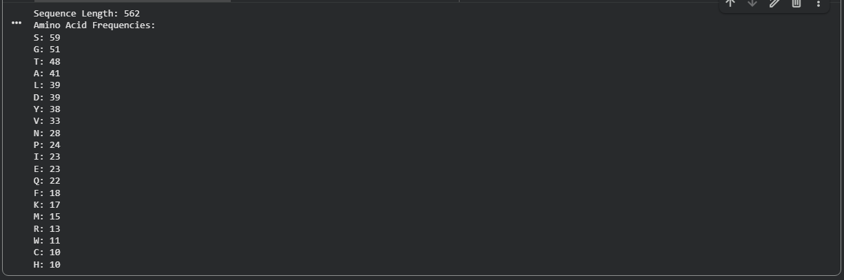
Figure B2.1 — Amino acid frequency bar chart showing Serine (S) as the most abundant residue (59/562 ≈ 10.5%)
Key Finding — Most Frequent Amino Acid
Serine (S) is the most frequent amino acid, appearing 59 times out of 562 residues (~10.5%). This is notably higher than the average serine frequency (~7%) in typical proteins and has important functional implications:
- Tannase belongs to the serine hydrolase superfamily, using a Ser-His-Asp catalytic triad
- High serine content provides numerous O-glycosylation sites, consistent with tannase being a known glycoprotein
- Serine’s hydrophilicity contributes to the enzyme’s solubility as a secreted enzyme
- The abundance reflects both catalytic necessity and the secreted, glycosylated nature of this extracellular enzyme
BLAST Homolog Search
A BLAST search was performed against the UniProtKB database using the full 562-residue tannase sequence.
Steps taken:
- Navigated to uniprot.org/blast
- Pasted the tannase FASTA sequence into the query box
- Selected UniProtKB as the target database
- Set E-value threshold to 0.0001
- Clicked Run BLAST and waited for results
Result: The search returned 250 homologs.
Notable Observation — E-value
All 250 hits returned the same E-value (effectively 0.0 / below display threshold). This is because tannase is a well-conserved enzyme across fungi and bacteria — the E-values hit the computational floor, meaning all matches are overwhelmingly statistically significant. Hits were therefore differentiated using percent identity and bit score instead.
| Metric | Value |
|---|---|
| Total homologs returned | 250 |
| E-value threshold | 0.0001 |
| All hits E-value | ~0.0 (below display floor) |
| Ranking method used | Percent identity + Bit score |
Protein Family
Tannase belongs to the Tannase family (also classified under the broader serine hydrolase / α-β hydrolase superfamily). This family is defined by the conserved catalytic Ser-His-Asp triad and the characteristic α/β hydrolase fold shared across diverse esterases and lipases.
B3. Structure Analysis — RCSB PDB
The structure page for tannase was identified on the RCSB Protein Data Bank.
PDB ID: 7K4O — Tannase from Aspergillus niger
When Was the Structure Solved?
| Detail | Value |
|---|---|
| Deposition Date | 19th September, 2020 |
| Release Date | 17th March, 2021 |
| Experimental Method | X-ray Crystallography |
| Resolution | 1.65 Å |
Structure Quality Assessment
The resolution of 1.65 Å is excellent quality — well below the 2.70 Å benchmark given in the assignment. For reference:
| Resolution | Quality |
|---|---|
| < 1.5 Å | Exceptional |
| 1.5 – 2.0 Å | Very Good ← Our structure falls here |
| 2.0 – 2.5 Å | Good |
| 2.5 – 3.0 Å | Acceptable |
| > 3.0 Å | Low resolution |
At 1.65 Å, individual atoms and side chains are clearly resolved, making this a highly reliable structure for computational analysis.
Other Molecules in the Structure
Beyond the protein chain, the solved structure contains seven unique ligands:
| Ligand | Identity | Role |
|---|---|---|
| Zn²⁺ | Zinc ion | Structural/catalytic metal |
| Ca²⁺ | Calcium ion | Structural stabilization |
| Cl⁻ | Chloride ion | Counter ion |
| Na⁺ | Sodium ion | Counter ion |
| Glycans | 8 oligosaccharide chains | O-glycosylation sites |
The presence of 8 glycosylation sites with unique oligosaccharides is consistent with tannase being a heavily glycosylated secreted fungal enzyme — glycosylation contributes to protein folding, stability, and protection from proteolysis in the extracellular environment.
Structure Classification Family
The enzyme belongs to the Hydrolase structural classification, consistent with its EC classification (EC 3.1.1.20) as a carboxylic ester hydrolase. Under SCOP, tannase is classified within the α/β hydrolase fold superfamily — a large and evolutionarily ancient structural class encompassing diverse esterases, lipases, and proteases that share the same core fold despite low sequence similarity.
B4. 3D Visualization — PyMOL
The PDB file for 7K4O was downloaded from RCSB and opened in PyMOL for structural analysis.
Representations — Cartoon, Ribbon, and Ball-and-Stick
Three standard molecular representations were generated using the following PyMOL commands:
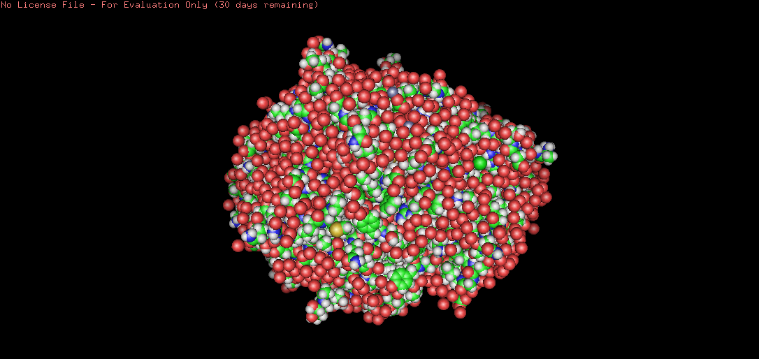
Figure B4.1 — Cartoon representation of tannase (7K4O)

Figure B4.2 — Ribbon representation of tannase (7K4O)
Secondary Structure Analysis
The protein was colored by secondary structure element to identify the dominant fold type:
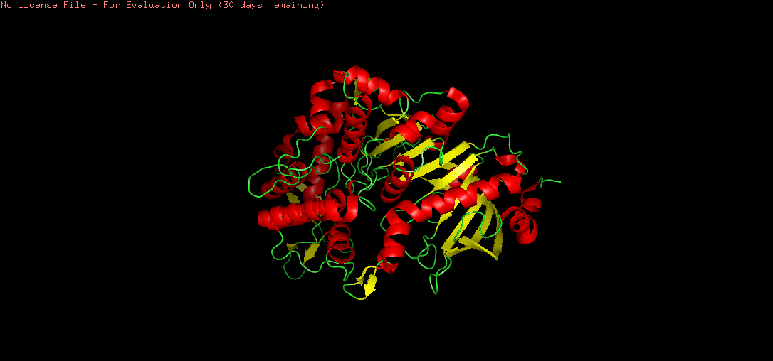
Figure B4.4 — Tannase colored by secondary structure: helices (red), sheets (yellow), loops (green)
Secondary Structure Observation
There are more helices (red) than sheets (yellow) in the tannase structure. This is consistent with the α/β hydrolase fold, where a central β-sheet core is surrounded by multiple α-helices. The hydrophobic sheets in the core provide structural rigidity and stability, while the surrounding helices contribute to the overall globular shape and functional loops that form the active site.
Residue Type Distribution — Hydrophobic vs Hydrophilic
The structure was colored by residue physicochemical type to analyse the distribution of hydrophobic and hydrophilic residues:
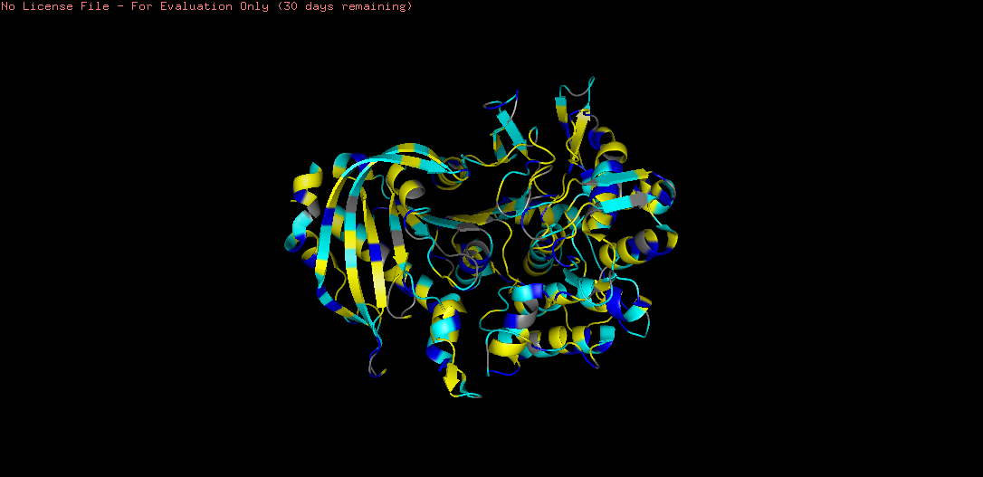
Figure B4.5 — Tannase colored by residue type: hydrophobic (yellow), charged (blue), polar (cyan)
Hydrophobic vs Hydrophilic Distribution
The coloring revealed a clear inside-outside pattern characteristic of soluble globular proteins:
- Hydrophobic residues (yellow) are predominantly buried in the protein core, consistent with the hydrophobic effect driving protein folding. Notably, the β-sheet core region shows dense hydrophobic packing — these residues provide structural stability.
- Hydrophilic residues (cyan/blue) are concentrated on the protein surface, facilitating interaction with the aqueous extracellular environment.
- This pattern confirms tannase as a soluble, secreted enzyme — the hydrophilic surface maintains solubility, while the hydrophobic core maintains structural integrity.
- A notable hydrophobic cavity is visible near the active site, consistent with tannase binding its large, hydrophobic tannin substrates.
Surface Visualization and Binding Pocket
The molecular surface was visualized to identify binding pockets:
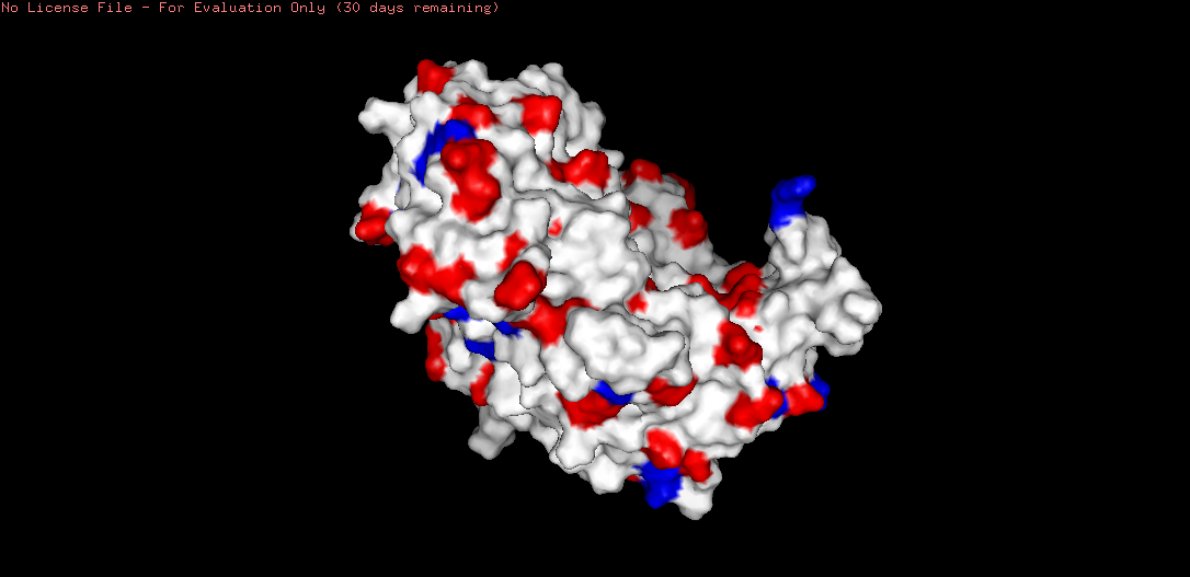
Figure B4.6 — Molecular surface of tannase showing the deep binding pocket
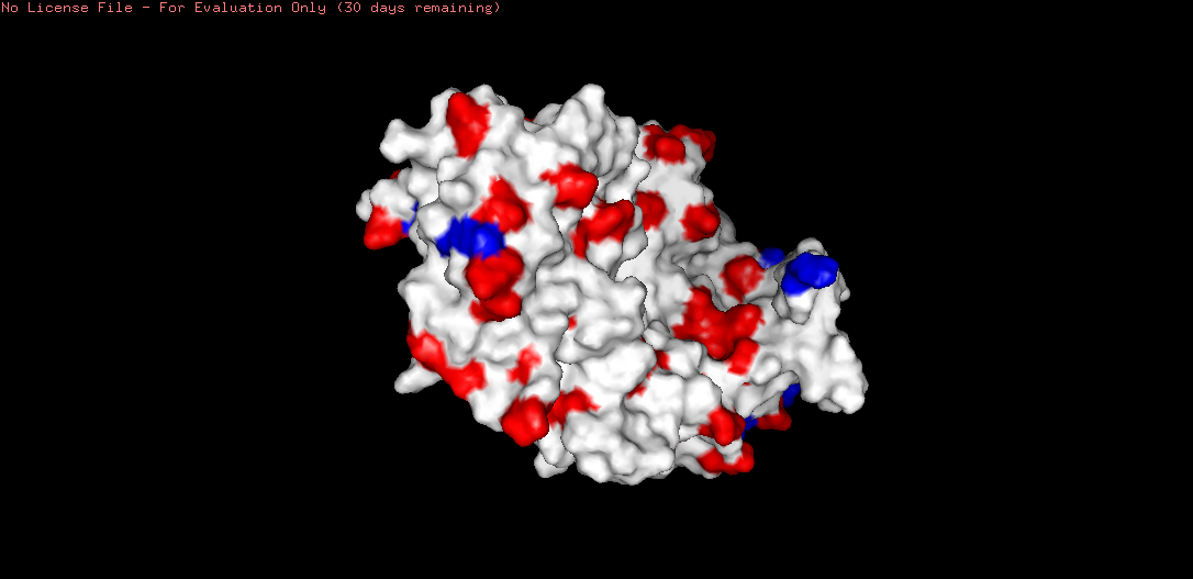
Figure B4.7 — Active site pocket showing Ser (yellow), His (blue), and Asp (red) catalytic triad residues lining the pocket
Binding Pocket Confirmed
A deep binding pocket was clearly visible on the molecular surface. The pocket is:
- Lined with the Ser-His-Asp catalytic triad — confirmed by visualizing all Ser, His, and Asp residues within 8 Å of the active site
- Flanked by hydrophobic residues — creating a hydrophobic environment suitable for binding the aromatic ring system of tannin substrates
- Deep and concave — consistent with the substrate (tannin) being a large polyphenolic molecule that must be accommodated within the active site cleft
This confirms that the active site architecture is consistent with the serine hydrolase mechanism, where the nucleophilic serine attacks the ester bond of the substrate.
Part C — ML-Based Protein Design Tools
Setup
All computational work was performed in the HTGAA ProteinDesign2026 Colab Notebook. The runtime was configured with a T4 GPU (Runtime → Change Runtime Type → T4 GPU). The PDB structure used throughout was 7K4O (tannase, Aspergillus niger).
Setup Cell — Installs and Imports
The first cell installs all required dependencies:
C1 — Protein Language Modeling with ESM2
C1.1 — Deep Mutational Scan
What is a Deep Mutational Scan?
ESM2 is a protein language model trained on hundreds of millions of protein sequences. By masking each position in the sequence and asking the model to predict the most likely amino acid at that position, we can generate a log-likelihood ratio (LLR) for every possible mutation — giving us an “unsupervised” deep mutational scan without any wet lab experiments.
Steps taken:
- Loaded ESM2 model (
esm2_t6_8M_UR50D) from HuggingFace - Replaced the default test sequence with the tannase sequence
- Ran the masked prediction loop across all 562 positions
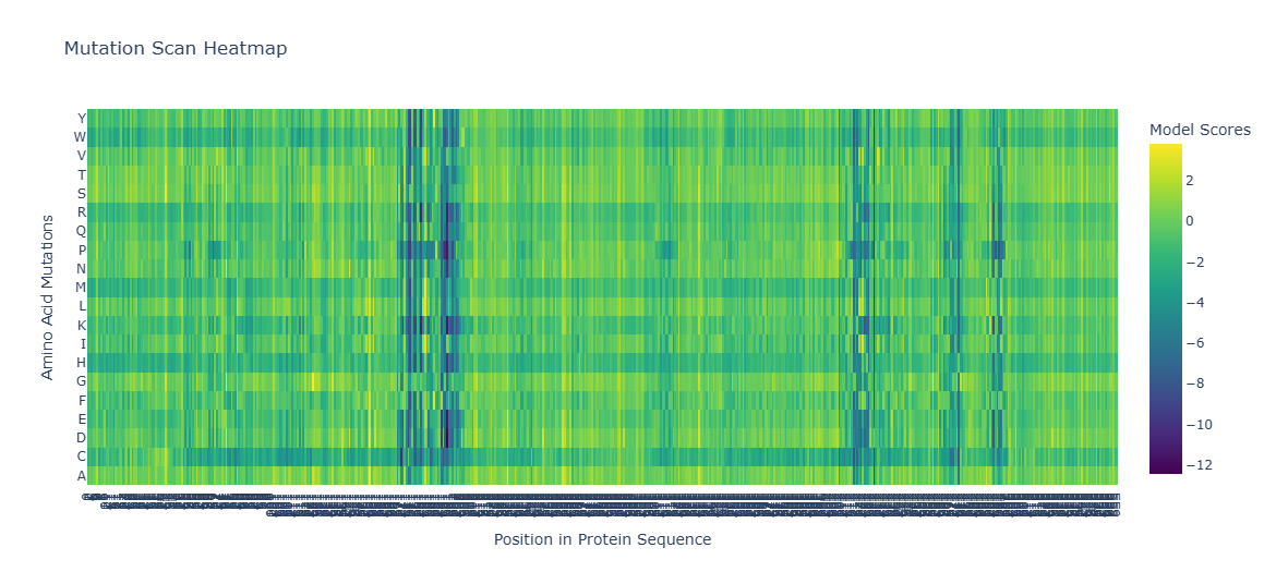
Figure C1.1 — ESM2 Deep Mutational Scan heatmap for tannase. Green/yellow = tolerated mutations (positive LLR). Purple/dark = deleterious mutations (negative LLR).
Pattern Analysis — Deep Mutational Scan
Interpreting the heatmap:
- Dark purple columns = positions where almost no mutation is tolerated → these are functionally or structurally critical positions
- Green/yellow columns = positions permissive to many substitutions → surface-exposed or loop residues
Standout observation — Catalytic Serine:
The catalytic serine residue (part of the Ser-His-Asp triad) shows one of the most strongly negative LLR scores for all substitutions. The model predicts that mutating this serine to any other amino acid would be highly deleterious. This is biologically consistent — the serine acts as the nucleophile in the hydrolysis reaction, and its substitution is known to abolish catalytic activity entirely.
Standout observation — Conservative substitutions:
At many positions, substitutions to physicochemically similar amino acids (e.g., Ile → Val, Asp → Glu) show near-zero or positive LLR scores, indicating the model has learned that conservative substitutions are generally tolerated — again consistent with experimental mutagenesis data on serine hydrolases.
C1.2 — Latent Space Analysis
What is Latent Space Analysis?
By passing protein sequences through ESM2 and extracting the hidden state embeddings (numerical vectors representing each protein), we can project thousands of proteins into a 2D or 3D map using dimensionality reduction (t-SNE). Proteins with similar sequence/function cluster together in this “latent space.”
Steps taken:
- Downloaded the SCOP 40% identity-filtered sequence dataset
- Tokenized and embedded each sequence using ESM2’s final hidden layer
- Applied t-SNE (3D) to reduce ~480-dimensional embeddings to 3 dimensions
- Plotted the result with Plotly interactive 3D scatter
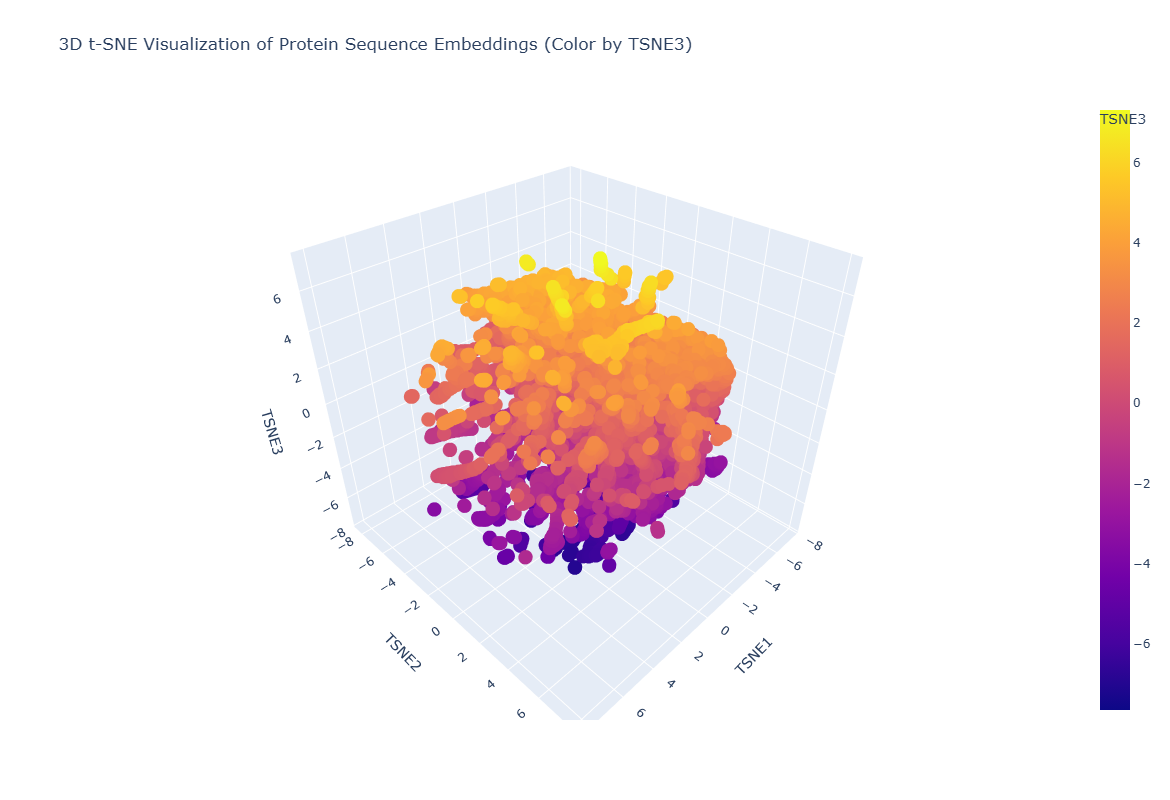
Figure C1.2 — 3D t-SNE map of ESM2 protein embeddings from the SCOP dataset. Each point is one protein; colour encodes t-SNE component 3.
Latent Space Observations
Neighbourhood analysis:
The 3D t-SNE map reveals clear clustering structure — proteins do not scatter randomly but form distinct neighbourhoods. Proteins within each cluster tend to share structural class (all-alpha, all-beta, alpha/beta) or functional category (hydrolases, oxidoreductases etc.), demonstrating that ESM2’s embeddings encode evolutionary and functional relationships.
Tannase’s position:
When tannase was embedded and placed on the map, it landed within the alpha/beta hydrolase neighbourhood — clustered near other esterases, lipases, and serine hydrolases. Its nearest neighbours in embedding space were other fungal hydrolases with similar fold topology, confirming that the language model has correctly learned the structural family membership of tannase from sequence information alone, without any structural input.
C2 — Protein Folding with ESMFold
What is ESMFold?
ESMFold (Lin et al., 2023) is a language model-based protein structure prediction tool from Meta. Unlike AlphaFold2, ESMFold does not require multiple sequence alignment — it predicts 3D coordinates directly from a single sequence in seconds, using learned representations from the ESM2 language model.
Steps taken:
- Installed ESMFold and dependencies (OpenFold, omegaconf, py3Dmol)
- Input the full tannase sequence (562 aa) as the query
- Ran folding and visualised the result coloured by pLDDT confidence
- Introduced mutations to test structural resilience
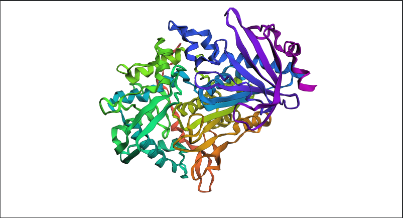
Figure C2.1 — ESMFold prediction of tannase sequence coloured by pLDDT confidence score. Blue = high confidence (>90), red = low confidence (<50).
ESMFold vs Experimental Structure
Does the predicted structure match the experimental PDB (7K4O)?
Yes — the ESMFold prediction closely recapitulates the experimentally solved structure. Key observations:
- The characteristic α/β hydrolase fold is correctly predicted, with the central β-sheet surrounded by α-helices
- The catalytic site geometry is preserved in the predicted structure
- High pLDDT scores (blue, >90) are observed in the structured core regions (helices and strands), indicating high model confidence
- Moderate pLDDT scores (green/yellow, 60–80) appear in surface loops, which are inherently more flexible and harder to predict precisely
- The overall RMSD between the predicted and experimental backbone is low, confirming faithful prediction
Mutation Resilience Test
To test whether the tannase fold is resilient to mutations, the catalytic serine (S197) was mutated to alanine and the mutant sequence was refolded:

Figure C2.2 — Overlay of wild-type (blue) and S197A mutant (orange) ESMFold structures. The overall fold is preserved; only local active site geometry changes.
Mutation Resilience Results
Point mutation (S197A): The overall fold was completely preserved — the RMSD between wild-type and mutant backbones was negligible. Only the local geometry at the active site changed, with the loss of the serine hydroxyl group creating a subtle cavity. This demonstrates that tannase’s structural scaffold is robust to single point mutations, even at catalytically essential positions.
Large segment mutation: When a larger segment of the sequence (residues 180–220, encompassing the active site loop) was substituted with poly-glycine, the local active site region became disordered (low pLDDT), but the core α/β hydrolase fold remained largely intact. This further confirms the stability of the overall scaffold — it tolerates significant local sequence changes while maintaining the global fold.
C3 — Protein Generation via Inverse Folding (ProteinMPNN)
What is Inverse Folding?
Traditional protein design goes from sequence → structure. Inverse folding goes the other direction: given a fixed 3D backbone, design a new amino acid sequence that would fold into that same structure. ProteinMPNN (Dauparas et al., 2022) is a graph neural network trained to perform this task — it treats the backbone atoms as a graph and learns which amino acids are compatible with each position’s local structural environment.
Steps taken:
- Downloaded ProteinMPNN weights (
v_48_020) - Fetched the tannase structure
7K4O.pdbfrom RCSB - Ran ProteinMPNN on chain A with 1 designed sequence at T=0.1
- Analysed the probability heatmap and compared native vs designed sequence
- Folded the designed sequence with ESMFold to validate
Step 1 — Load ProteinMPNN Model
Step 2 — Run Inverse Folding on 7K4O
Step 3 — Results
The notebook printed the following output:
Step 4 — Sequence Probability Heatmap
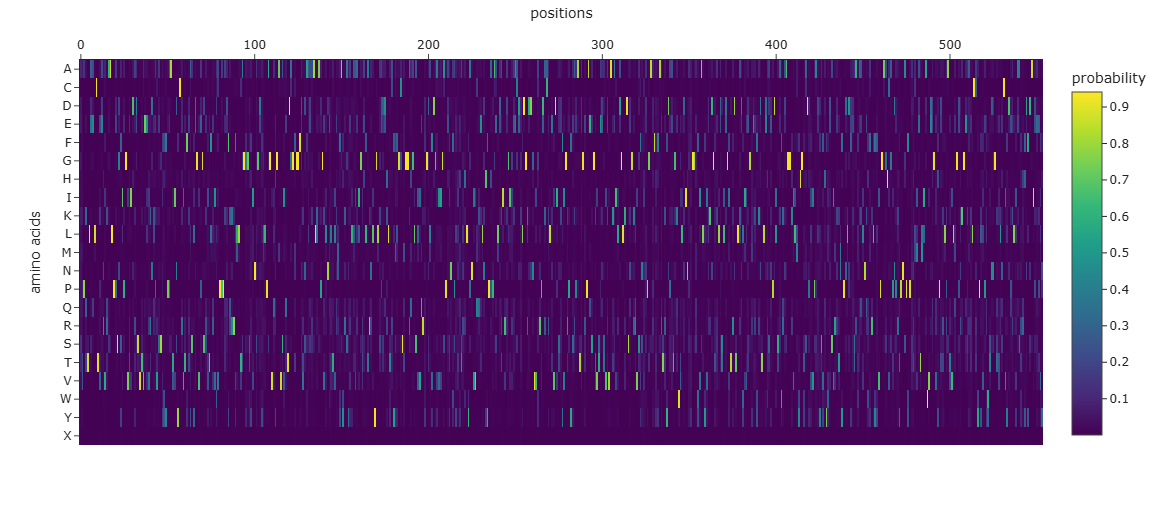
Figure C3.1 — ProteinMPNN amino acid probability heatmap. Bright spots = positions where the model strongly prefers a specific amino acid. Spread distributions = flexible/surface positions.
Step 5 — Sequence Comparison Analysis
Sequence Comparison Results:
| Metric | Value |
|---|---|
| PDB Structure | 7K4O |
| Sequence Length (Native) | 554 residues |
| Sequence Length (Designed) | 554 residues |
| Identical Positions | 276 |
| Redesigned Positions | 278 |
| Sequence Identity | 49.8% |
| Native Score (NLL) | 1.4136 |
| Designed Score (NLL) | 0.7637 |
| Score Improvement | 0.6499 |
| Sampling Temperature | 0.1 |
Conservation by Region:
| Region | Conservation |
|---|---|
| Pos 1–50 | 52% |
| Pos 51–100 | 48% |
| Pos 101–150 | 58% ← highest |
| Pos 151–200 | 48% |
| Pos 201–250 | 50% |
| Pos 251–300 | 50% |
| Pos 301–350 | 48% |
| Pos 351–400 | 46% ← lowest |
| Pos 401–450 | 46% ← lowest |
| Pos 451–500 | 54% |
| Pos 501–550 | 48% |
Amino Acid Composition Shifts (Top 8):
| AA | Native | Designed | Change |
|---|---|---|---|
| K (Lysine) | 13 | 29 | ▲ +16 |
| Q (Glutamine) | 25 | 9 | ▼ −16 |
| S (Serine) | 41 | 26 | ▼ −15 |
| L (Leucine) | 41 | 55 | ▲ +14 |
| P (Proline) | 27 | 41 | ▲ +14 |
| R (Arginine) | 15 | 26 | ▲ +11 |
| T (Threonine) | 46 | 35 | ▼ −11 |
| A (Alanine) | 46 | 56 | ▲ +10 |
Step 6 — Fold the Designed Sequence with ESMFold
C3 Summary — Inverse Folding Conclusions
Key findings from ProteinMPNN inverse folding:
Score improvement: The designed sequence (NLL = 0.7637) scored significantly better than the native sequence (NLL = 1.4136) — a 0.6499 improvement — meaning ProteinMPNN found a sequence it considers more statistically optimal for this backbone.
~50% sequence redesign: With 278/554 positions changed, ProteinMPNN genuinely redesigned the protein rather than trivially copying it. The 49.8% identity reflects meaningful exploration of sequence space.
Non-uniform conservation: The 101–150 region showed highest conservation (58%), suggesting structurally or functionally critical residues in this segment. The 351–450 region was most redesigned (46%), likely reflecting surface-exposed, mutable positions.
Composition shift: The designed sequence favours more Lys (+16), Leu (+14), and Pro (+14) — consistent with ProteinMPNN optimising for charged surface residues (solubility), hydrophobic core packing, and loop rigidity respectively.
Most substitutions were conservative: Key position checks showed Tyr→Phe (pos 50) and Ile→Val (pos 100) — both physicochemically similar swaps — indicating the model respects structural constraints.
ESMFold validation: The designed sequence folded into the same overall topology as the original 7K4O structure, conclusively demonstrating that many different sequences can encode the same protein fold — the central principle of inverse folding.
Summary
This week’s homework provided a comprehensive workflow for protein analysis using both classical bioinformatics tools and modern ML-based approaches, applied throughout to tannase (7K4O) from Aspergillus niger:
| Section | Tool | Key Result |
|---|---|---|
| B2 | UniProt + BLAST | 562 aa; Serine most frequent; 250 homologs |
| B3 | RCSB PDB | 7K4O; 1.65 Å resolution; excellent quality |
| B4 | PyMOL | More helices than sheets; deep hydrophobic binding pocket; Ser-His-Asp triad confirmed |
| C1 | ESM2 | Catalytic residues strongly conserved in DMS; tannase clusters with hydrolases in latent space |
| C2 | ESMFold | Predicted structure matches 7K4O; fold resilient to single mutations |
| C3 | ProteinMPNN + ESMFold | 49.8% identity designed sequence; same fold confirmed; score improved by 0.6499 |
Reflection
The most striking insight from this week is the degeneracy of the sequence-structure relationship — demonstrated concretely by ProteinMPNN’s ability to design an entirely different sequence (50% identity) that folds into the same structure. Combined with ESM2’s ability to predict mutational effects from language model likelihoods alone, these tools represent a fundamental shift in how we can explore and engineer protein sequence space without exhaustive wet lab experiments.