Turning Trash into Treasure with Synthetic Biology
Hello! I’m Peter Olawumi (@dev_roc on X), a software developer based in Ibadan, Nigeria. With a passion for innovative solutions at the intersection of technology, hardware, and biology, I’m excited to be part of How to Grow (Almost) Anything 2026. My background in coding fuels my drive to create accessible tools for real-world problems, especially in developing regions like the Global South.
My Final Project: Microbial “Plastic Eater” Pods for Factory-Floor Recycling
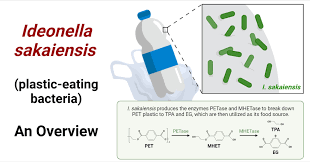
Picture a bustling Lagos factory overwhelmed by PET plastic waste. My project aims to engineer Ideonella sakaiensis bacteria into supercharged “plastic eaters” housed in compact, on-site pods. These lunchbox-sized bioreactors will break down PET scraps into reusable monomers at ambient temperatures, reducing waste transport emissions by 40% and fostering a circular economy.
Why This Matters
In Nigeria, plastic pollution clogs waterways and harms health. Traditional recycling is energy-intensive and inefficient. My bioengineered solution uses optimized enzymes (PETase & MHETase) for faster degradation, with built-in safeties like kill switches to prevent ecological risks.
Technical Highlights
Enzyme Engineering: Codon-optimized genes with secretion signals and GFP reporters.
Workflow: In silico design (AlphaFold).
Governance & Ethics
Ensuring ethical deployment is key. My goals focus on biosafety (containment mechanisms) and equity (open-source designs). Proposed actions include regulatory certifications, subsidies, and sentinel networks—balancing innovation with responsibility.
HTGAA 2026 – Week 4 homework: Protein Design Part I (Conceptual Questions, Protein Analysis & Visualization, ML-Based Design Tools, and Group Brainstorm)
HTGAA Spring 2026 | Week 5 Homework Designing peptide binders for A4V SOD1 and engineering MS2 L-protein mutants using protein language models and structural prediction.
Part A — SOD1 Binder Peptide Design Target: Superoxide dismutase 1 (SOD1) carrying the A4V mutation (Ala→Val at residue 4), which causes familial ALS by destabilising the N-terminus and promoting toxic aggregation.
Assignment: DNA Assembly Question 1 — Components of the Phusion High-Fidelity PCR Master Mix and Their Purpose The Phusion HF PCR Master Mix is a pre-formulated 2X concentrate containing all enzymatic and chemical components needed for PCR. Only template, primers, and nuclease-free water need to be added by the researcher. Its key components are:
Assignment Part 1: Intracellular Artificial Neural Networks (IANNs) Question 1: Advantages of IANNs over traditional Boolean genetic circuits Traditional genetic circuits compute Boolean functions — AND, OR, NAND, NOR — where each input is treated as fully on or fully off, and the output is discrete. This binary logic imposes a hard constraint: the circuit cannot distinguish how much of a signal is present, only whether it is present. IANNs overcome this and several related limitations.
Subsections of Homework
Week 1: Principles & Practices
About Me
My name is Peter Olawumi, and I’m based in Ibadan, Nigeria. As a software developer, I’m passionate about bridging technology and biology to create innovative, accessible solutions for real-world problems, especially in the Global South. Joining HTGAA is an exciting opportunity to explore synthetic biology and apply it to challenges like waste management in our growing industrial sectors.
Proposed Biological Engineering Application or Tool
I propose developing microbial “Plastic Eater” pods for on-site industrial recycling. These are compact, factory-floor bioreactors using engineered bacteria to break down PET plastic waste into reusable monomers.
Why this? In bustling manufacturing plants in Lagos and Ibadan, discarded PET bottles and packaging pile up daily, leading to costly hauling, environmental pollution, and health risks from microplastics. Traditional recycling is energy-intensive and inefficient, with global rates at just 18%. In Nigeria, informal recycling dominates but lags in efficiency. My tool would be a lunchbox-sized pod that processes 500g-1kg of PET scraps per cycle at ambient temperatures, yielding 80-90% monomer recovery (terephthalic acid and ethylene glycol) for repolymerization or new chemicals. It’s low-energy, scalable, and deployable without shipping, inspired by natural degraders like Ideonella sakaiensis, supercharged with synthetic biology for faster action.
The core: Engineer Ideonella sakaiensis or a surrogate like Pseudomonas putida with optimized PETase and MHETase enzymes, fused to secretion signals and reporters for efficiency. This could cut waste transport emissions by 40%, create bio-recycling jobs, and align with UN SDG 12 for sustainable consumption.
Governance/Policy Goals
To ensure this tool contributes to an ethical future, I focus on non-malfeasance (preventing harm). I’ve adapted the synthetic genomics framework for safety/security and equity.
Goal 1: Biosafety Lockdown – Prevent Unintended Microbial Escapes and Toxicity This goal contains recombinant strains to avoid ecological disruptions, like outcompeting native microbes or leaching toxins in biodiverse areas like Lagos lagoons.
Sub-goal 1a: Engineered Containment Mechanisms – Integrate two orthogonal kill switches (e.g., mazEF toxin-antitoxin and light-inducible CRISPRi) in plasmids. Validate with in vitro escape assays (>99.99% die-off in 48 hours via qPCR).
Sub-goal 1c: Toxicity Profiling for Byproducts and Enzymes – Conduct assays on outputs (Ames test for genotoxicity <2x induction; yeast screen for endocrine disruption EC50 >100μM). Cap enzyme secretion to avoid risks.
Goal 2: Equitable Deployment – Ensure Broad Access Without Widening Industrial Divides This prevents social harms like job displacement, promoting inclusive scaling inspired by the African Union’s biotech equity charter.
Sub-goal 2a: Open-Source IP and Tech Transfer – Classify designs as Creative Commons (CC-BY-SA) for non-commercial use in developing economies. Host on iGEM registry with modular parts for local adaptations.
Sub-goal 2b: Socio-Economic Impact Audits – Use agent-based modeling (NetLogo) to forecast job shifts (e.g., aim for Gini coefficient drop <0.1). Include community “right-to-reject” via town halls (>60% approval).
Sub-goal 2c: Adaptive Monitoring for Long-Term Equity – Integrate IoT sensors into pods for blockchain-ledger yield tracking (70% monomer value back to operators). Cap market share (<30%) to avoid over-reliance.
Governance Actions
I’ve outlined three actions: a regulatory rule, an incentive program, and a technical strategy, involving different actors. Analogies draw from drones (certification), finance (buffers), and 3D printing (open designs).
Action 1: Mandatory Pre-Deployment “Escape-Proof” Certification (Regulatory Rule by Federal Agencies) Analogy: FAA drone certification for safe airspace.
Purpose: Current Nigerian biosafety (NBMA 2015 Act) is ad-hoc, risking spills. Propose standardized “synbio passport” with <0.01% escape risk proven via simulations, shifting to proactive approvals.
Design: Amend Biosafety Regulations (2020) for dossiers (COPASI models, assays, audits). Actors: NBMA approves (6-month review); companies fund (₦500k-1M, offset by permits); academics validate. Use open API for data.
Assumptions: Regulators have capacity (50+ assessors); models translate to real-world (e.g., floods); industry complies without loopholes.
Action 2: “Green Pod” Subsidy Incentives with Equity Audits (Incentive Program by Industry-Academia Consortia) Analogy: Basel III capital buffers for financial resilience.
Purpose: Factories prioritize profits over equity; propose 40% tax credits for adopters passing audits (30% revenue shared with informal sectors), shifting to impact investing.
Design: Co-designed by MAN/universities, funded by 1% levy (₦10B pot). Actors: Companies self-audit (NetLogo); consortia approve; NGOs monitor. Use blockchain for payouts; train 1k workers/year.
Assumptions: Big firms lead (70% pilot adoption); audits capture nuances; economic stability holds.
Action 3: Open-Source “Watchdog” Microbial Sentinel Network (Technical Strategy by Academic Researchers) Analogy: Thingiverse for 3D printing with safety mods.
Purpose: Fragmented tracking leaves surveillance gaps; propose free platform with sentinel kits (qPCR for HGT) for crowdsourced monitoring, shifting to community-driven oversight.
Design: Led by UNILAG/iGEM Africa with $500k grants. Actors: Researchers upload (CC-BY); factories deploy ($50/unit); NBMA integrates. Use Raspberry Pi/ML for alerts; beta in HTGAA, then 100-node pilot.
Assumptions: Open-source thrives (1k contributors); low-tech adoption; data privacy holds.
Using an adapted rubric (1 = best/strong positive, 3 = weak/neutral, n/a = not applicable):
Does the option:
Action 1
Action 2
Action 3
Enhance Biosecurity
• By preventing incidents
1
2
1
• By helping respond
2
3
1
Foster Lab Safety
• By preventing incidents
1
n/a
2
• By helping respond
2
n/a
1
Protect the Environment
• By preventing incidents
1
2
2
• By helping respond
2
3
1
Promote Equity
• By ensuring access
3
1
2
• By minimizing divides
3
1
2
Other Considerations
• Minimize costs/burdens
2
1
1
• Feasibility
2
2
1
• Not impede research
3
2
1
• Promote constructive apps
2
1
2
Explanation: Action 1 excels in prevention but burdens innovation (higher costs). Action 2 boosts equity and feasibility via incentives but weaker on direct security. Action 3 is feasible and responsive but risks privacy issues.
Prioritization and Trade-offs
I prioritize a combination of Action 2 (incentives) and Action 3 (sentinel network), starting with academics and industry consortia, targeted at national audiences like Nigeria’s Ministry of Science & Technology and international like the African Union. Why? This balances proactive equity (Action 2’s audits prevent divides) with responsive monitoring (Action 3’s crowdsourcing flags harms early), scoring well on feasibility and constructive uses without heavy regulation that could slow adoption in resource-limited settings.
Trade-offs: Incentives may increase short-term costs (levy) but yield long-term savings (20% waste reduction); open-source risks IP theft but promotes access. Assumptions: Strong community buy-in (e.g., 70% SME uptake); uncertainties include enforcement in informal sectors and tech literacy. If unaddressed, fall back to Action 1 for high-risk deployments.
Reflection on Class Learnings
From lectures by David Kong, George Church, and Joe Jacobson, I learned about biotech’s rapid evolution and ethical imperatives like biosecurity and equity. A new concern for me: In the Global South, unequal access could exacerbate divides—e.g., advanced tools benefiting only elites. Another: Dual-use risks, where degraders might be misused for harmful polymers.
To address: Propose mandatory equity clauses in grants (e.g., 20% project budget for community training) and international standards for dual-use reviews (adapt WHO guidelines). This ties to my project, emphasizing open designs with built-in safeties.
Lecture 2 Preparation – Homework Answers
For Professor Jacobson Lecture
Error Rate of Polymerase
The error rate of nature’s DNA polymerase (specifically, error-correcting polymerase in biological synthesis) is approximately 1 error per 10⁹ (1 billion) base pairs added.
The human genome is roughly 3 × 10⁹ (3 billion) base pairs long. This means that, on average, DNA replication of the entire human genome would introduce about 3 errors per replication cycle if relying solely on this error rate.
Biology addresses this discrepancy through multiple layers of error correction and repair mechanisms beyond the base polymerase error rate. These include:
Built-in proofreading via 3’–5’ exonuclease activity in the polymerase itself, which immediately detects and corrects mismatches during synthesis.
Post-replication mismatch repair systems that scan for and fix errors shortly after replication.
Additional DNA repair pathways (e.g., base excision repair, nucleotide excision repair, and double-strand break repair) that operate continuously to detect and correct damage from replication errors, environmental factors, or spontaneous mutations.
These combined mechanisms can reduce the effective mutation rate to as low as 10⁻¹⁰ per base pair in vivo, ensuring genome stability across cell divisions.
Number of Ways to Code for an Average Human Protein
An average human protein is encoded by approximately 1036 base pairs of DNA, corresponding to about 345 amino acids (since each amino acid is coded by a 3-base codon, or triplet).
The genetic code uses 64 possible codons (4³) to specify 20 amino acids and 3 stop signals. Excluding stop codons, there are 61 codons for the 20 amino acids, yielding an average degeneracy of about 3.05 codons per amino acid.
For a specific protein sequence of 345 amino acids, the total number of different DNA nucleotide sequences (coding sequences) that could translate to the exact same amino acid sequence is enormous — on the order of 3.05³⁴⁵ ≈ 10¹⁶⁷.
In practice, not all of these theoretically possible coding sequences work effectively to produce the protein of interest (especially in the context of gene synthesis and expression). Important limiting factors include:
Codon usage bias — different organisms prefer certain synonymous codons due to tRNA abundance
mRNA secondary structure and stability (hairpins, degradation signals)
Synthesis errors — chemical DNA synthesis has higher error rates (~1:10² per base)
Regulatory constraints (e.g., in recoded organisms with codon reassignment)
Functional impacts of synonymous changes on folding, translation kinetics, and expression levels
For these reasons, synthetic genes are usually designed with a subset of “optimal” codons rather than exploring the full theoretical space.
For Dr. LeProust Lecture
Most Commonly Used Method for Oligo Synthesis Currently
The most commonly used method for oligonucleotide (oligo) synthesis is solid-phase phosphoramidite chemistry.
This involves a cyclic process on a solid support (controlled pore glass or silicon-based chips, as used by Twist Bioscience):
Coupling — DMT-protected phosphoramidite monomer is added to the growing chain
Capping — Unreacted sites are capped to prevent further extension
Oxidation — Phosphite linkage is oxidized to a stable phosphate
Deblocking — DMT group is removed to allow the next coupling
This method, developed in the early 1980s, remains the industry standard for automated, high-throughput oligo synthesis.
Why It Is Difficult to Make Oligos Longer Than 200 nt Via Direct Synthesis
Direct chemical synthesis of oligos longer than ~200 nucleotides is challenging primarily due to the limitations of coupling efficiency in phosphoramidite chemistry (typically 98–99% per step).
For a 200 nt oligo, theoretical yield of full-length product is approximately (0.99)¹⁹⁹ ≈ 13%, but in practice it is significantly lower due to accumulating side reactions such as:
Depurination (acid-induced base loss)
Incomplete deprotection
Branching and other side products
These issues cause exponential yield drop and increasing error accumulation (deletions, insertions, substitutions), making purification of full-length, error-free products very difficult beyond ~200 nt.
While advanced platforms (e.g. Twist Bioscience) have improved chemistry to routinely reach ~350 nt and demonstrated ~700 nt experimentally (with ~97% full-length material), these are not standard for direct synthesis beyond 200 nt.
Why You Can’t Make a 2000 bp Gene Via Direct Oligo Synthesis
A 2000 base pair gene cannot be made via direct oligo synthesis because current chemical methods are fundamentally limited in length (routine max ~350 nt, experimental ~700 nt).
Attempting 2000 bp directly would result in near-zero yield due to:
Extremely low coupling efficiency over thousands of steps → theoretical yield (0.99)¹⁹⁹⁹ ≈ 10⁻⁹ (practically nonexistent)
Massive accumulation of chemical errors (depurination, oxidation byproducts, etc.)
Impractical purification at that scale
Instead, genes of this length are constructed by assembling multiple shorter oligos (typically 50–300 nt) using enzymatic methods such as:
Gibson assembly
Enzymatic assembly platforms (e.g. Twist HELIX2)
Followed by cloning, error correction, and verification via long-read sequencing
This modular approach overcomes the direct synthesis length barrier.
For George Church Lecture
Suggested Code for AA:AA Interactions
For AA:AA (amino acid–amino acid) interactions in proteins — which enable folding, oligomerization, and interfaces (analogous to NA:NA basepairing or AA:NA ribosomal translation) — I suggest a Side Chain Complementarity Code based on physicochemical properties of amino acid side chains.
This probabilistic code categorizes preferred pairings:
Hydrophobic–Hydrophobic — van der Waals forces (e.g. Leu ↔ Ile, Val ↔ Phe) → core stabilization, coiled-coils, β-sheets
Special / covalent — disulfide bonds (Cys ↔ Cys), metal coordination (e.g. His ↔ His via Zn²⁺)
This framework aligns with natural protein interaction rules and could be extended for synthetic biology applications, e.g. incorporating non-standard amino acids to create novel interaction pairs.
In recitation, we discussed that you will pick a protein for your homework that you find interesting. Which protein have you chosen and why? Using one of the tools described in recitation (NCBI, UniProt, google), obtain the protein sequence for the protein you chose
The protein I have chosen for the homework is PETase (poly(ethylene terephthalate) hydrolase) from the bacterium Piscinibacter sakaiensis (previously known as Ideonella sakaiensis).
I find this protein particularly interesting because it represents a breakthrough in addressing one of the world’s major environmental challenges: plastic pollution. PETase is an enzyme that can break down polyethylene terephthalate (PET), a common plastic used in bottles, packaging, and textiles. Discovered in a bacterium isolated from plastic waste, PETase enables the microbe to use PET as a carbon and energy source by hydrolyzing its ester bonds. This natural biological degradation process offers hope for sustainable recycling and bioremediation of plastics, unlike traditional mechanical or chemical methods that are energy-intensive or produce pollutants. The enzyme’s specificity for PET and its activity at relatively mild temperatures also make it exciting for potential biotechnological applications, such as engineered variants for industrial plastic breakdown.
Using UniProt (one of the tools mentioned in recitation for protein information), I retrieved the protein sequence for PETase from Piscinibacter sakaiensis. The UniProt accession is A0A0K8P6T7, and here is the full amino acid sequence (290 residues):
3.2. Reverse Translate: Protein (amino acid) sequence to DNA (nucleotide) sequence.
The Central Dogma discussed in class and recitation describes the process in which DNA sequence becomes transcribed and translated into protein. The Central Dogma gives us the framework to work backward from a given protein sequence and infer the DNA sequence that the protein is derived from. Using one of the tools discussed in class, NCBI or online tools (google “reverse translation tools”), determine the nucleotide sequence that corresponds to the protein sequence you chose above.
Once the nucleotide sequence of your protein is determined, you need to codon optimize your sequence. You may, once again, utilize Google for a “codon optimization tool”.
In your own words, describe why do you need to optimize codon usage. Which organism have you chose to optimize the codon sequence for and why?
Optimization is vital to achieve improvements in protein synthesis efficiency, either in terms of stability, structure, and speed of the processes. This is achieved by employing specific codons that are preferred by the organism of interest. This translates into increased protein expression.
In this case, I selected Escherichia coli , one of the model organisms in protein production in biotechnology. The preference is associated with the ease of manipulation of its genes and rapid proliferation/growth as it is an organism that is not very demanding in terms of conditions. This makes it an ideal organism for this type of experiments.
3.4. You have a sequence! Now what?
What technologies could be used to produce this protein from your DNA? Describe in your words the DNA sequence can be transcribed and translated into your protein. You may describe either cell-dependent or cell-free methods, or both.
In this case, it is possible to use both methods:
Cell-free methods: based on the use of cell extracts or synthetic compounds with the ability to perform translation and transcription by having the respective machinery (ribosomes, RNA polymerase, etc.), without the need for living cells. These are usually encapsulated in cell-free protein synthesis systems (CFPs), capable of producing proteins that are collected directly. An example of this is through the use of a system that incorporates the preparation of a bacterial lysate and encapsulation in vesicles. There are also commercial CFPs kits that could be used to produce a protein of interest.
Cell-dependent methods: based on the use of live cells, in this case it is possible to work with plasmids for the production of recombinant proteins in E. coli . One of the most widely used series in recent years is the pET line, allowing efficient protein translation. In these systems, the incorporated machinery of the cells is what allows these processes to be executed, and it is also necessary to have: a DNA sequence, a terminator, a regulatory sequence, ARN polymerase, enhancers, and start and termination codons, among others. In addition to the insertion of the gene or genes, it is also necessary to carry out bacterial transformation processes, induce expression, and finally extract the purified protein.
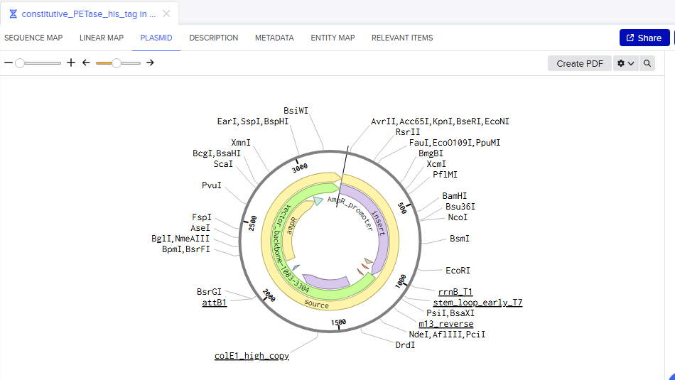
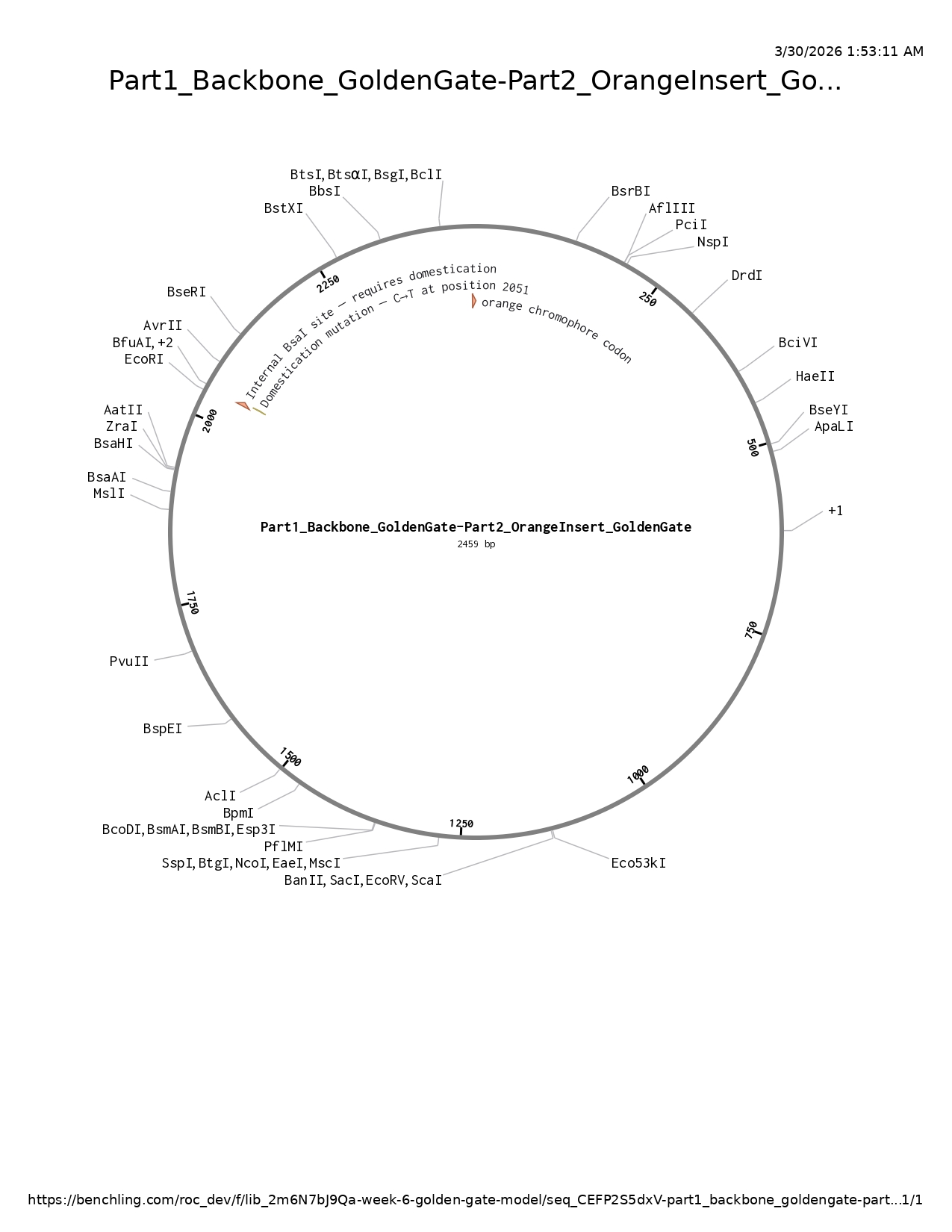
Part 4: My first Benchling plasmid 🧬
Part 5: DNA Read/Write/Edit
5.1 DNA Read
(i) What DNA would you want to sequence (e.g., read) and why? This could be DNA related to human health (e.g. genes related to disease research), environmental monitoring (e.g., sewage waste water, biodiversity analysis), and beyond (e.g. DNA data storage, biobank).
I consider that it could be of interest to work with the eae gene of the enteropathogenic pathotype of E. coli (EPEC), responsible for encoding the intimin protein, necessary for adherence to the intestinal epithelium and which causes diarrheal affections as a consequence worldwide. This could be very useful for environmental monitoring and the study of epidemiological patterns in developing countries such as Ecuador. Since it is one of the main pathogens of public health risk, sequencing is proposed as an alternative for the study in complex environments such as river waters or important sources of high contamination.
(ii) In lecture, a variety of sequencing technologies were mentioned. What technology or technologies would you use to perform sequencing on your DNA and why? Also answer the following questions:
a. Is your method first-, second- or third-generation or other? How so?
The first-generation Sanger method is proposed for this case. It is positioned in this category as one of the first methods used in DNA sequencing in 1977. It is based on the addition of deoxynucleotides that facilitate DNA chain elongation. It is also useful in this case because of its accuracy, ease, cost, and, above all, because the size of the strand of interest is manageable for the technology (881bp).
b. What is your input? How do you prepare your input (e.g. fragmentation, adapter ligation, PCR)? List the essential steps.
Extraction of DNA from study samples (e.g. contaminated water). The use of an extraction kit is suggested to ensure higher purity of the sample and avoid other contaminants.
Performing a conventional PCR to obtain an adequate amount of the fragment, ensuring that it is in a pure form. Only PCR conventional components are required as normal nucleotides (dNTPs) and a thermostable DNA polymerase (Taq polymerase).
c. What are the essential steps of your chosen sequencing technology, how does it decode the bases of your DNA sample (base calling)?
For Sanger sequencing the DNA obtained from PCR is mixed with other reagents: nucleotides (dNTPs) and other special nucleotides that are fluorescently labeled (ddNTPs).
The polymerase then synthesizes a new strand and when a ddNTP is added, the process is stopped, resulting in fragments of different lengths.
These fragments are separated in a capillary electrophoresis process where the shorter fragments migrate faster and in turn, the fragments are excited by a laser which emits a specific signal for each fragment.
These signals can then be recorded by a detector and translated into a nucleotide sequence.
d. What is the output of your chosen sequencing technology?
The method generates an electropherogram, which is a graph showing the fluorescence peaks corresponding to each nucleotide in the DNA sequence. Where each color represents a specific base (A, T, C, G).
5.2 DNA Write
(i) What DNA would you want to synthesize (e.g., write) and why? These could be individual genes, clusters of genes or genetic circuits, whole genomes, and beyond. As described in class thus far, applications could range from therapeutics and drug discovery (e.g., mRNA vaccines and therapies) to novel biomaterials (e.g. structural proteins), to sensors (e.g., genetic circuits for sensing and responding to inflammation, environmental stimuli, etc.), to art (DNA origamis). If possible, include the specific genetic sequence(s) of what you would like to synthesize! You will have the opportunity to actually have Twist synthesize these DNA constructs! :)
For this section, I would be interested in synthesizing DNA associated with Shiga toxin as the Stx2 responsible for multiple outbreaks at the global level and the cause of hemolytic uremic syndrome. This toxin is usually produced by serotypes of pathogenic E. coli ( STEC), so its synthesis could be of interest in the development of recombinant vaccines, by obtaining attenuated antigens.
(ii) What technology or technologies would you use to perform this DNA synthesis and why? Also, answer the following questions:
I would make use of the Gibson Assembly technology because it is highly accurate and efficient compared to others such as Golden Gate, and I consider this to be essential in vaccine development. In addition, it is sufficiently suitable for the assembly of a plasmid with an attenuated version of the toxin and is flexible in case modifications are necessary to improve the immune response.
What are the essential steps of your chosen sequencing methods?
In the first instance, it is necessary to synthesize or amplify an attenuated version of the protein (toxin) of interest. This means removing the domains or parts associated with toxicity but retaining the elements that activate the immune response in patient’s body. This gene can be obtained by PCR and must have overlapping ends that match the plasmid where the insertion will be made.
The plasmid to be used is also pre-designed and linearized to facilitate insertion.
The next step is the assembly, which consists of mixing these components in a tube with Gibson’s mix containing: exonuclease responsible for generating the overlapping ends, polymerase that fills these spaces, and ligase that joins these fragments.
Finally, the next step is the transformation of the organism chosen, in this case, E. coli, by the addition of this recombinant plasmid.
b. What are the limitations of your sequencing method (if any) in terms of speed, accuracy, and scalability?
Among the limitations of this method are the possible formation of secondary structures and the need for long overlapping sequences which could lead to complications in the design and synthesis. The cost could also be relatively high compared to the other alternatives.
5.3 DNA Edit.
(i) What DNA would you want to edit and why? In class, George shared a variety of ways to edit the genes and genomes of humans and other organisms. Such DNA editing technologies have profound implications for human health, development, and even human longevity and human augmentation. DNA editing is also already commonly leveraged for flora and fauna, for example in nature conservation efforts, (animal/plant restoration, de-extinction), or in agriculture (e.g. plant breeding, nitrogen fixation). What kinds of edits might you want to make to DNA (e.g., human genomes and beyond) and why?
For this part of the paper, I would again bring up the idea of modifying the genes of plants that are subject to desiccation problems such as bananas. I believe that the agricultural sector in countries like Ecuador has great potential to test these technologies and improve yield and productivity levels.
(ii) What technology or technologies would you use to perform these DNA edits and why? Also answer the following questions:
How does your technology of choice edit DNA? What are the essential steps?
It starts with the design of the construct of interest, in this case consisting of the DREB1A gene, which is inserted into an expression vector together with its promoter.
This vector is then introduced into A. tumefaciens and the plants of interest are infected in an in vitro culture, which will allow the integration of the gene of interest. The principle of this technology is based on the ability of this bacterium to transfer DNA to other cells, using its Ti plasmid in which the region associated with the tumors is replaced by the region of interest. Thus, when this bacterium infects plant tissue, this genetic alteration is also transferred.
Subsequently, the plants that have been transformed correctly are selected, this can be through a fluorescent marker such as GFP.
Additionally, expression tests can be performed by RT-qPCR, and lastly, the regeneration and re-planting of the culture of interest is performed.
b. What preparation do you need to do (e.g. design steps) and what is the input (e.g. DNA template, enzymes, plasmids, primers, guides, cells) for the editing?
This process requires the selected gene of interest, a suitable vector compatible with A. tumefaciens including a promoter, terminator, and selection marker. Also, designed primers, restriction enzymes, ligases, culture media, and growth hormones.
c. What are the limitations of your editing methods (if any) in terms of efficiency or precision?
The main limitations revolve around the efficacy of the transformation because it is subject to a process of transgenesis, which could compromise the specificity and accuracy of the editing. In addition to possible unwanted adverse effects due to random insertions.
1. Published Paper Using Opentrons for Novel Biological Applications
One compelling example is the paper “Semi-automated Production of Cell-Free Biosensors” by Dylan M. Brown, Daniel A. Phillips, and colleagues (bioRxiv preprint October 13, 2024; formally published in ACS Synthetic Biology, 2025).
The team used the affordable Opentrons OT-2 liquid-handling robot to scale up manufacturing of cell-free synthetic biology biosensors for point-of-need diagnostics (e.g., detecting fluoride in drinking water). They developed a semi-automated protocol that precisely assembles viscous cell-free reaction mixes (DNA template + PANOx extract + buffers) into full 384-well plates in ~30 minutes—something that was previously done manually with high operator-to-operator variability.
Key novel application: They created and lyophilized hundreds of identical fluoride-riboswitch biosensors that can be rehydrated in the field and give a clear colorimetric or fluorescent readout. By optimizing robot parameters (dispense height, mix volume, aspiration rate), they achieved reproducibility that matched or exceeded manual assembly while drastically reducing hands-on time and batch-to-batch variation. This opens the door to cheap, deployable diagnostics in low-resource settings (they reference prior field tests in Kenya and Costa Rica). The work is especially elegant because it shows how open-source automation turns cell-free systems from lab curiosities into manufacturable products—exactly the kind of scalability we need in synthetic biology.
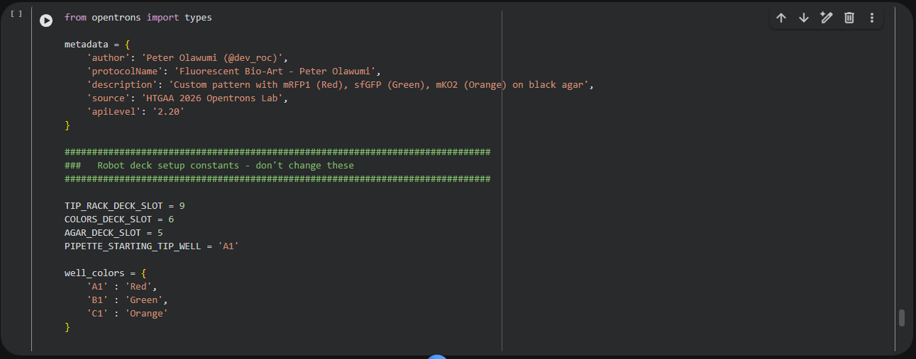
2. What I Intend to Do with Automation Tools for My Final Project
Project Title: Microbial “Plastic Eaters” – Engineering On-Site Industrial Recycling Pods with Recombinant PETase/MHETase in a Cell-Free + Bacterial Pipeline
My final project builds a portable “recycling pod” that uses engineered bacteria (or their secreted enzymes) to break down PET plastic waste directly on factory floors. The bottleneck is rapid optimization of PETase and MHETase variants for faster degradation, higher temperature tolerance, and better secretion. Automation will let me screen dozens-to-hundreds of variants in parallel, run degradation assays remotely, and iterate in days instead of weeks.
Here is exactly what I plan to automate:
A. High-Throughput Variant Library Assembly & Cell-Free Expression Screening (Primary automation goal – inspired by the cell-free biosensor paper above)
Opentrons OT-2 (or cloud lab equivalent) will perform Golden Gate assembly of PETase mutant libraries (active-site saturation + secretion-signal variants).
Echo transfer or Opentrons p20 multi-channel will dispense 50–100 ng of each linearized plasmid + cofactors into 96-well or 384-well plates.
Bravo / Opentrons stamps in the cell-free protein synthesis (CFPS) master mix (E. coli lysate + energy components).
Multiflo dispenses the full reaction volume to start expression.
PlateLoc seals the plate.
Inheco or Opentrons temperature module incubates at 30 °C / 37 °C for 4–16 h.
XPeel removes seal.
PHERAstar or plate reader measures either (a) fluorescence (GFP-fused PETase) or (b) enzymatic activity via p-nitrophenyl ester surrogate substrate at 405 nm.
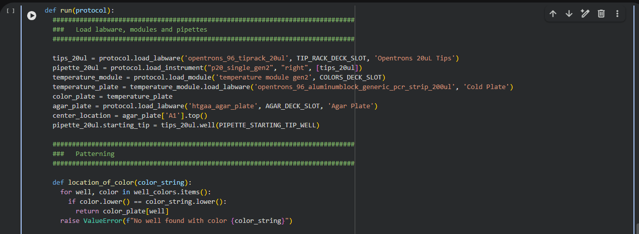
Pseudocode / Opentrons Python sketch:
fromopentronsimportprotocol_apimetadata={'apiLevel':'2.15'}defrun(protocol:protocol_api.ProtocolContext):# Labwaretiprack=protocol.load_labware('opentrons_96_tiprack_20ul',1)source_plate=protocol.load_labware('nest_96_wellplate_200ul_flat',2)# DNA variantscfps_plate=protocol.load_labware('nest_96_wellplate_200ul_flat',3)temp_module=protocol.load_module('temperature module gen2',4)temp_module.set_temperature(30)p20=protocol.load_instrument('p20_multi_gen2','left',tip_racks=[tiprack])# Step 1: Transfer DNA variantsforcolinrange(8):# 8 columns = 96 variantsp20.pick_up_tip()p20.transfer(2,source_plate.columns()[col],cfps_plate.columns()[col],mix_after=(3,10))p20.drop_tip()# Step 2: Add CFPS master mix (multi-channel)p20.pick_up_tip()p20.distribute(18,master_mix_reservoir,cfps_plate.wells(),disposal_volume=5)p20.drop_tip()# Incubate & read laterprotocol.pause("Incubate 6 h at 30 °C")
B. 3D-Printed Custom Holders (from Opentrons 3D Printing Directory style) I will design and print (using the class Prusa or lab printer) a PET-flake assay tray: a 96-well-compatible holder that securely positions 5 mm × 5 mm shredded PET flakes or thin PET film strips at the bottom of each well. The holder has sloped walls and a mesh bottom so supernatant can be easily aspirated for downstream HPLC or weight-loss measurements without losing plastic particles. This turns a messy manual assay into a clean, robot-friendly 96-well format.
C. Cloud-Lab Integration (Ginkgo Nebula / similar remote biofoundry) Once top variants are identified on the Opentrons, I will upload the best 10–20 constructs to Ginkgo Nebula (or equivalent cloud laboratory) for larger-scale bacterial expression and real PET degradation in 1 L bioreactors. The cloud lab will:
Run parallel fermentations with automated sampling.
Perform continuous OD600, pH, and TPA/EG monomer quantification via inline HPLC.
Return lyophilized enzyme powders ready for pod prototyping.
D. Full Degradation Validation Loop After cell-free hits, Opentrons will set up 24–48 replicate mini-reactions with purified enzyme + real factory PET scraps, incubate with shaking, and automatically sample at 0/24/48/72 h for mass-loss and LC-MS readout. This closed loop (design → assemble → express → assay → analyze) will run with minimal intervention, letting me test 50+ variants per week.
By combining the Opentrons for precision liquid handling, 3D-printed custom labware for PET-specific assays, and cloud-lab scale-up, I will move from gene sequence to validated high-performance enzyme cocktail in a matter of weeks—exactly what an industrial recycling pod needs. This automation plan directly mirrors the cell-free biosensor paper’s success in scaling reproducible reactions and will make my project robust, repeatable, and genuinely ready for Lagos factory floors.
Week 4: Protein Design Part I
This week focuses on how sequence, structure, and energetics can be modeled and manipulated to create or optimize proteins with specified functions.
Lecture (Tues, Feb 24)
Lab (Thurs-Fri, Feb 26 - 27)
Lab work this week is contained within the homework assignment below.
Homework: Protein Design I — DUE BY START OF MAR 3 LECTURE
Objective:
Learn basic concepts: • amino acid structure • 3D protein visualization • the variety of ML-based design tools
Brainstorm as a group how to apply these tools to engineer a better bacteriophage (setting the stage for the final project).
Part A. Conceptual Questions
Assignees for this section
MIT/Harvard students
Required
Committed Listeners
Required
Answer any NINE of the following questions from Shuguang Zhang: (i.e. you can select two to skip)
Question 1 — How many amino acid molecules are in 500 g of meat?
Red meat contains roughly 28 g of protein per 100 g, so 500 g of meat contains approximately 140 g of protein.
Using the given average amino acid molecular weight of ~100 Da (100 g/mol):
$$
N = n \times N_A = 1.4 \times 6.022 \times 10^{23} \approx \boxed{8.4 \times 10^{23} \text{ molecules}}
$$
That is nearly one full mole of amino acid molecules — comparable to Avogadro’s number itself. The remaining mass of the meat (water, fat, connective tissue) accounts for why we use ~28% protein content rather than 100%.
Question 2 — Why don’t you become a cow when you eat beef?
When you eat beef, your digestive system completely dismantles its proteins before anything is absorbed. Proteases in the stomach (pepsin, activated at pH ~2) and the small intestine (trypsin, chymotrypsin, elastase) hydrolyze all peptide bonds, reducing every protein — no matter its origin — down to free amino acids or small di- and tripeptides.
These building blocks are then absorbed into the bloodstream and delivered to your ribosomes, which read your mRNA, which was transcribed from your DNA. Your cells reassemble the amino acids into human proteins according to your own genetic blueprint. The sequence information encoded in the beef protein is destroyed during digestion and never enters your cells.
This follows directly from the Central Dogma of molecular biology: information flows DNA → RNA → Protein, and there is no pathway for dietary protein sequence to be reverse-translated back into nucleic acid and incorporated into your genome.
Key principle
You absorb the chemical raw materials (amino acids), not the sequence information. The genetic identity of food is completely lost in the gut.
Question 3 — Why are there only 20 natural amino acids?
This is one of biology’s most debated open questions. Several complementary hypotheses exist:
1. The frozen accident hypothesis (Crick, 1968)
The canonical 20 may be largely arbitrary — an early selection that became irreversibly locked in. Once the genetic code was embedded in the proteomes of early life, any mutation that altered codon assignments would catastrophically mis-fold thousands of proteins simultaneously. The code froze before it could be revised, trapping whatever 20 happened to be in use.
2. Chemical space coverage
The 20 amino acids collectively cover a remarkably diverse chemical space: hydrophobics (Val, Leu, Ile, Phe, Met), polar uncharged (Ser, Thr, Asn, Gln, Cys, Tyr), positively charged (Lys, Arg, His), negatively charged (Asp, Glu), and the structurally special Gly and Pro. This palette is sufficient for nucleophilic catalysis, metal coordination, hydrogen bonding, and hydrophobic packing — essentially all enzyme chemistry.
3. Codon constraint
The standard genetic code has 64 codons (4³). Encoding 20 amino acids with 3 stop codons allows substantial redundancy (degeneracy), which buffers point mutations. Adding more amino acids would require new codon assignments and would conflict with existing reading frames.
4. Biosynthetic accessibility
All 20 are derived from just a handful of central metabolic intermediates (pyruvate, oxaloacetate, α-ketoglutarate, 3-phosphoglycerate, phosphoenolpyruvate, erythrose-4-phosphate, ribose-5-phosphate). This makes them cheap to synthesize and plausibly available in a prebiotic world.
The most likely answer is a combination: a small set was prebiotically available, early proto-life settled on it, and evolutionary lock-in prevented expansion.
Question 4 — Can you make non-natural amino acids? Design some.
Yes — non-natural amino acids (nnAAs) are a well-established field of chemical biology. All amino acids share the backbone:
Engineering a new amino acid means designing a novel R-group (side chain) attached to that Cα. They can be incorporated into proteins using amber codon suppression: the UAG stop codon is reassigned to the nnAA using an engineered orthogonal tRNA / aminoacyl-tRNA synthetase pair (pioneered by Schultz and others).
Known examples
Amino acid
Side chain
Application
Azidohomoalanine (AHA)
–(CH₂)₃–N₃
Azide handle for copper-free click chemistry bioconjugation
p-Acetylphenylalanine
–C₆H₄–C(=O)–CH₃
Ketone handle for oxime ligation with hydroxylamine probes
The electron-withdrawing fluorines tune vinyl reactivity, making this a potential mechanism-based inhibitor for PLP-dependent enzymes (acting as a Michael acceptor at the active site). The C–F bonds also confer metabolic stability against oxidative degradation. Backbone: standard L-α configuration.
Design B — Bipyridyl alanine
Side chain: $\text{–CH}_2\text{–(2,2’-bipyridyl)}$
A bipyridine side chain coordinates transition metals (Fe²⁺, Cu²⁺, Ni²⁺) with high affinity. Incorporating this into a designed metalloenzyme would install a programmable metal-binding site with precise geometric control, enabling redox catalysis or FRET-based metal sensing.
Practical note
nnAAs can now be incorporated in living cells using engineered pyrrolysyl-tRNA synthetase (PylRS) variants, which have a large, flexible active site that tolerates diverse side chains. Directed evolution of PylRS is the primary route to activating new nnAAs in vivo.
Question 5 — Where did amino acids come from before enzymes, before life?
Three well-evidenced abiotic routes produced amino acids on early Earth:
1. Spark discharge — the Miller-Urey experiment (1953)
Stanley Miller and Harold Urey demonstrated that passing electrical discharges (simulating lightning) through a reducing atmosphere of CH₄, NH₃, H₂O, and H₂ produces amino acids spontaneously. The experiment yielded glycine, alanine, aspartate, glutamate and more — all without any enzyme. Later analyses of the original sealed flasks found over 20 amino acids in total.
2. Meteoritic delivery
Carbonaceous chondrite meteorites (Murchison, Murray, Allende) contain over 70 different amino acids, including non-biological ones (D-isomers, β-amino acids, unusual side chains). These are synthesized by Strecker reactions in interstellar ice grains and delivered intact to planetary surfaces. The Murchison meteorite, which fell in Australia in 1969, remains the best-characterized source of extraterrestrial amino acids.
3. Hydrothermal vents
Alkaline deep-sea hydrothermal vents (like the Lost City field) provide H₂, CO₂, heat, and iron-sulfur mineral catalysts that can drive amino acid synthesis via Fischer-Tropsch-type reactions. The mineral surfaces act as primitive catalysts, mimicking what enzymes do today.
4. HCN chemistry (Strecker synthesis)
HCN (hydrogen cyanide), abundant on early Earth and in comets, reacts with aldehydes and ammonia:
This Strecker pathway produces α-amino acids from simple one-carbon feedstocks with no biological machinery required.
Question 6 — If you build an α-helix from D-amino acids, what handedness would it have?
A helix made entirely of D-amino acids would be left-handed.
Here is why. The handedness of a protein helix is determined by the stereochemistry at the Cα of each residue, which constrains the backbone dihedral angles φ and ψ.
Amino acid type
Favored φ, ψ
Helix sense
L-amino acids
φ ≈ −57°, ψ ≈ −47°
Right-handed α-helix
D-amino acids
φ ≈ +57°, ψ ≈ +47°
Left-handed α-helix
D-amino acids are the mirror image of L-amino acids. The mirror image of a right-handed helix is a left-handed helix. These left-handed D-peptide helices have been synthesized experimentally and are used in mirror-image protein engineering — a strategy where entire proteins are assembled from D-amino acids to produce their enantiomeric “mirror” counterparts. These mirror proteins are completely resistant to natural proteases (which have L-amino acid active sites and cannot recognize the D-peptide backbone), making them highly stable therapeutics.
Question 7 — Can you discover additional helices in proteins?
Beyond the canonical α-helix, several other helical structures exist in proteins:
graph TD
    H[Protein helices] --> A[α-helix\ni to i+4 H-bond\n3.6 res/turn\nRight-handed]
    H --> B[3₁₀-helix\ni to i+3 H-bond\n3.0 res/turn\nTighter]
    H --> C[π-helix\ni to i+5 H-bond\n4.4 res/turn\nWider]
    H --> D[Polyproline II\nNo H-bonds\nLeft-handed\nExtended]
    H --> E[Collagen triple helix\nInterchain H-bonds\nGly-X-Y repeat]
    H --> F[β-helix\nβ-strands coiling\ninto a solenoid]
3₁₀-helix: Hydrogen bonds between residue i and i+3 (tighter than α). Found at the C-terminal ends of α-helices. About 10–15% of all helical residues in proteins are 3₁₀.
π-helix: Hydrogen bonds between i and i+5, with a wider diameter than α. Rare (~1% of helical residues) but enriched at functionally important sites — often near ligand-binding regions.
Polyproline II (PPII) helix: A left-handed helix with no intramolecular hydrogen bonds (φ ≈ −75°, ψ ≈ +145°). Abundant in collagen, intrinsically disordered regions, and signaling peptides (SH3 domain binding sites).
β-helix: β-strands wind into a helical solenoid. Found in pectate lyase, some carbonic anhydrases, and many bacterial virulence factors. Two sub-types: parallel (all strands same direction) and antiparallel.
Tools like DSSP (Define Secondary Structure of Proteins) and Ramachandran plot analysis can be used to search the PDB for non-canonical helices by identifying backbone dihedral angles that fall outside the classic α-helix basin.
Question 8 — Why are most molecular helices right-handed?
The prevalence of right-handed helices in biology traces directly to the homochirality of L-amino acids. This operates at two levels:
Stereochemical level: L-amino acids have backbone dihedral angles favoring φ ≈ −57°, ψ ≈ −47°. In a right-handed helix, side chains point outward and avoid steric clashes with backbone carbonyls. Attempting to form a left-handed α-helix with L-amino acids generates severe steric clashes between side chains and carbonyl oxygens (except for glycine, which has no side chain and can access both regions of the Ramachandran plot).
Origin of L-homochirality: Several competing hypotheses exist:
Circularly polarized light (CPL): Neutron stars and pulsars emit CPL, which may have preferentially photodegraded D-amino acids in interstellar space before Earth’s formation, seeding a small initial L-excess
Chiral mineral surfaces: Calcite and quartz surfaces can preferentially adsorb one enantiomer
Autocatalytic amplification (Soai reaction): A small initial chiral excess can be amplified to near-homochirality through autocatalytic chemistry
Once life committed to L-amino acids, right-handed helices became the universal default and were evolutionarily locked in — exactly as the genetic code itself was frozen.
Outside biology
In purely synthetic chemistry, both helical senses are equally stable. Peptides made from racemic mixtures of D/L amino acids do not form regular helices at all — regular secondary structure requires stereochemical consistency.
Question 9 — Why do β-sheets tend to aggregate?
The structural problem: exposed edge strands
A β-sheet is intrinsically “unfinished” on both edges. Interior strands satisfy all their backbone hydrogen bonds with neighbors on both sides, but the edge strands have a row of free NH donors and C=O acceptors pointing into solvent. These unsatisfied hydrogen bond groups create a thermodynamic driving force to recruit additional β-strands — ideally from another peptide chain.
Driving forces for aggregation
1. Hydrogen bonding at edges
Each edge strand presents a periodic array of H-bond donors and acceptors spaced ~4.7 Å apart — exactly complementary to another β-strand. The enthalpy gain from satisfying these groups (–2 to –5 kcal/mol per H-bond) drives lateral sheet association.
2. Hydrophobic stacking
β-sheets have one hydrophobic face (side chains pointing into a protein core) and one polar face. When two sheets associate, the hydrophobic faces pack against each other, releasing ordered water molecules and gaining entropy — the classic hydrophobic effect.
3. Extended backbone geometry
In a β-strand, φ ≈ −120°, ψ ≈ +120° — the backbone is nearly fully extended, maximizing exposure of both H-bond donors and acceptors. This is geometrically opposite to the α-helix, where backbone groups are buried in intramolecular H-bonds.
graph LR
    A[Free edge strand\nUnsatisfied H-bonds] -->|H-bond + hydrophobic| B[Sheet-sheet\ninterface]
    B --> C[Oligomeric\nproto-fibril]
    C -->|Nucleation-dependent\ngrowth| D[Amyloid fibril\nCross-β architecture]
In vivo consequence
Cells spend significant energy preventing β-sheet aggregation: chaperones (Hsp70, Hsp90, GroEL) bind exposed β-strands, prolines and charged residues are inserted at strategic positions to interrupt aggregation-prone sequences, and quality control pathways (UPS, autophagy) degrade aberrant aggregates.
Question 10 — Why do amyloid diseases form β-sheets? Can amyloid be used as a material?
Why amyloid = cross-β structure
Amyloid fibrils are built on cross-β architecture: individual β-strands run perpendicular to the fibril axis and stack along it with ~4.7 Å inter-strand spacing, hydrogen bonding collectively across thousands of stacked chains. This produces a thermodynamically extraordinary structure:
All backbone H-bonds are satisfied (no free edge strands — the fibril itself is the edge-propagating aggregate)
Hydrophobic side chains are buried in the fibril core
The structure is more stable than the native fold of the precursor protein in many cases
Many amyloidogenic proteins (Aβ in Alzheimer’s, α-synuclein in Parkinson’s, tau, prion protein PrP, transthyretin) contain intrinsically disordered regions or partially unfolded segments that are aggregation-prone. Under conditions of stress, mutation, aging, or elevated concentration, these segments nucleate β-strand assembly. Once a nucleus forms, elongation is thermodynamically downhill — each fibril end templates further monomer addition in a seeded polymerization mechanism.
Where the toxicity comes from
The mature fibrils are not necessarily the toxic species. Soluble oligomeric intermediates (2–50 mers) formed during the nucleation phase are increasingly recognized as the primary toxic agents, disrupting membranes, synaptic function, and cellular proteostasis.
Amyloid as a material
Yes — and this is an active research frontier. Amyloid fibrils have remarkable mechanical properties:
Property
Value
Comparison
Young’s modulus
~10–20 GPa
Comparable to steel (~200 GPa) or bone (~20 GPa)
Tensile strength
~0.1–1 GPa
Similar to silk fibers
Self-assembly
Spontaneous from peptide solution
No external machinery required
Fiber diameter
7–12 nm
True nanoscale
Applications under development:
Nanowires: Metal ion-doped amyloid fibrils (e.g., with silver or gold) conduct electricity along the fibril axis
Hydrogels: Cross-linked amyloid networks form tunable, biocompatible gels for tissue engineering scaffolds
Thin films: Amyloid monolayers on surfaces for biosensors and anti-fouling coatings
Living materials:E. coli naturally secretes curli fibers (a bacterial amyloid). The Joshi/Lu labs have engineered programmable curli networks where bacteria secrete functionalised amyloid on demand, acting as living, self-repairing materials
Question 11 — Design a β-sheet motif that forms a well-ordered structure
Design principles
A well-ordered β-sheet motif requires:
Alternating hydrophobic/polar pattern — one face hydrophobic for core packing, one face solvent-exposed and polar
β-branched residues (Val, Thr, Ile) to favor extended strand conformation and disfavor α-helix
Engineered turns to reverse strand direction with defined geometry
Edge protection to prevent uncontrolled aggregation
Position:   1   2   3   4   5   6   7
Residue:    V   T   V   T   V   T   V
Face:      HΦ  POL HΦ  POL HΦ  POL HΦ
Val (V) at odd positions: β-branched, strongly hydrophobic, disfavors α-helix (ΔΔG ~1 kcal/mol over Ala), forms the buried hydrophobic core face
Thr (T) at even positions: β-branched (stabilizes β-strand) with an –OH group for H-bonding on the solvent face; the methyl group contributes mild hydrophobicity
Turn 1 — D-P-G (Type II’ β-turn):
Asp (i): carbonyl oxygen accepts H-bond from the preceding strand’s NH, capping that edge
Pro (i+1): φ locked at ~−60° by ring constraint, ideal for the Type II’ turn geometry
Gly (i+2): no side chain, provides conformational flexibility for the reversal
Turn 2 — N-G-K (Type I β-turn):
Asn (i): amide side chain caps the turn with an additional H-bond
Gly (i+1): conformational flexibility
Lys (i+2): positive charge improves aqueous solubility and opposes the Asp charge from Turn 1
Schematic of hydrogen bond pattern (antiparallel)
Strand 1 →   V — T — V — T — V — T — V
             |       |       |       |     ← backbone H-bonds
Strand 2 ←   V — T — V — T — V — T — V
             |       |       |       |
Strand 3 →   V — T — V — T — V — T — V

Turn 1 (DPG) connects strand 1 → strand 2
Turn 2 (NGK) connects strand 2 → strand 3
Why this should form a well-ordered structure
The Val/Thr alternation is the same patterning principle used in the Woolfson group’s SAF (self-assembling fiber) peptides and Zhang’s EAK16/RADA16 ionic self-assembling peptides
Antiparallel geometry is thermodynamically preferred over parallel for short strands (better H-bond geometry, more favorable twist)
The DPG turn has been validated computationally and experimentally as a reliable β-hairpin nucleator (used in the Gellman lab’s β-hairpin model systems)
At pH 7, the Asp¹ (−1) and Lys² (+1) charges on the turns offset each other, minimizing net charge while maintaining solubility
Edge capping: the charged turn residues flanking the sheet introduce electrostatic repulsion between assembled sheets, limiting uncontrolled fiber growth and allowing formation of a discrete, soluble β-sheet rather than amyloid
Extending the design
To validate this motif computationally: (1) run a Rosetta FastRelax protocol with the sequence to check predicted backbone geometry, (2) verify that predicted φ/ψ angles fall in the β-sheet basin (φ ≈ −120°, ψ ≈ +120°) of the Ramachandran plot, (3) check for predicted burial of Val residues in the hydrophobic core, (4) use MD simulation (GROMACS/AMBER) to test stability in explicit water over 100 ns.
Objective
This week explores how sequence, structure, and energetics can be modelled and manipulated to create or optimize proteins with specified functions. I selected Tannase (Aspergillus niger) as my protein of interest throughout Parts B and C.
Part B — Protein Analysis and Visualization
B1. Protein Selection
I selected Tannase (Tannin acyl hydrolase; EC 3.1.1.20) from Aspergillus niger as my protein of interest for this assignment. Tannase is a fascinating extracellular enzyme that catalyzes the hydrolysis of ester and depside bonds in hydrolysable tannins, releasing gallic acid and glucose. My interest in this enzyme stems from two reasons: first, it aligns directly with my research focus in enzyme biotechnology; and second, its peculiar biochemical activity — degrading complex plant polyphenols — makes it a compelling subject for structural and computational analysis. Tannase has significant industrial applications in food processing, beverage clarification, and pharmaceutical production, which adds practical relevance to studying it computationally.
B2. Amino Acid Sequence Analysis
Sequence Retrieval
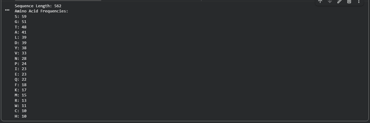
The amino acid sequence of Aspergillus niger tannase was retrieved from the UniProt database. The sequence is 562 amino acids long.
Figure B2.1 — Amino acid frequency bar chart showing Serine (S) as the most abundant residue (59/562 ≈ 10.5%)
Key Finding — Most Frequent Amino Acid
Serine (S) is the most frequent amino acid, appearing 59 times out of 562 residues (~10.5%). This is notably higher than the average serine frequency (~7%) in typical proteins and has important functional implications:
Tannase belongs to the serine hydrolase superfamily, using a Ser-His-Asp catalytic triad
High serine content provides numerous O-glycosylation sites, consistent with tannase being a known glycoprotein
Serine’s hydrophilicity contributes to the enzyme’s solubility as a secreted enzyme
The abundance reflects both catalytic necessity and the secreted, glycosylated nature of this extracellular enzyme
BLAST Homolog Search
A BLAST search was performed against the UniProtKB database using the full 562-residue tannase sequence.
Pasted the tannase FASTA sequence into the query box
Selected UniProtKB as the target database
Set E-value threshold to 0.0001
Clicked Run BLAST and waited for results
Result: The search returned 250 homologs.
Notable Observation — E-value
All 250 hits returned the same E-value (effectively 0.0 / below display threshold). This is because tannase is a well-conserved enzyme across fungi and bacteria — the E-values hit the computational floor, meaning all matches are overwhelmingly statistically significant. Hits were therefore differentiated using percent identity and bit score instead.
Metric
Value
Total homologs returned
250
E-value threshold
0.0001
All hits E-value
~0.0 (below display floor)
Ranking method used
Percent identity + Bit score
Protein Family
Tannase belongs to the Tannase family (also classified under the broader serine hydrolase / α-β hydrolase superfamily). This family is defined by the conserved catalytic Ser-His-Asp triad and the characteristic α/β hydrolase fold shared across diverse esterases and lipases.
The resolution of 1.65 Å is excellent quality — well below the 2.70 Å benchmark given in the assignment. For reference:
Resolution
Quality
< 1.5 Å
Exceptional
1.5 – 2.0 Å
Very Good ← Our structure falls here
2.0 – 2.5 Å
Good
2.5 – 3.0 Å
Acceptable
> 3.0 Å
Low resolution
At 1.65 Å, individual atoms and side chains are clearly resolved, making this a highly reliable structure for computational analysis.
Other Molecules in the Structure
Beyond the protein chain, the solved structure contains seven unique ligands:
Ligand
Identity
Role
Zn²⁺
Zinc ion
Structural/catalytic metal
Ca²⁺
Calcium ion
Structural stabilization
Cl⁻
Chloride ion
Counter ion
Na⁺
Sodium ion
Counter ion
Glycans
8 oligosaccharide chains
O-glycosylation sites
The presence of 8 glycosylation sites with unique oligosaccharides is consistent with tannase being a heavily glycosylated secreted fungal enzyme — glycosylation contributes to protein folding, stability, and protection from proteolysis in the extracellular environment.
Structure Classification Family
The enzyme belongs to the Hydrolase structural classification, consistent with its EC classification (EC 3.1.1.20) as a carboxylic ester hydrolase. Under SCOP, tannase is classified within the α/β hydrolase fold superfamily — a large and evolutionarily ancient structural class encompassing diverse esterases, lipases, and proteases that share the same core fold despite low sequence similarity.
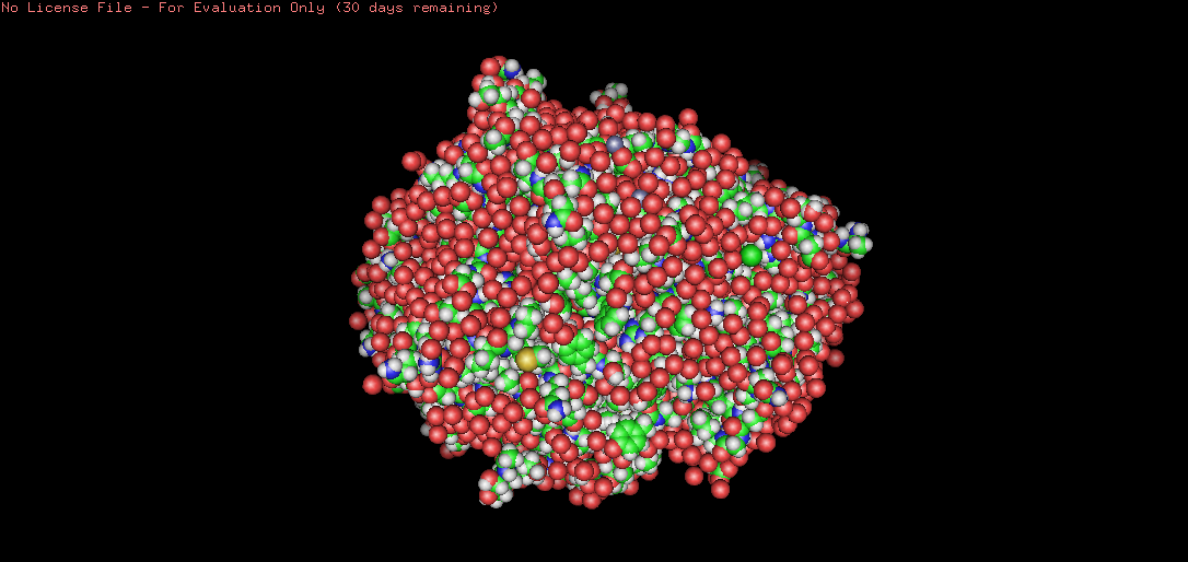
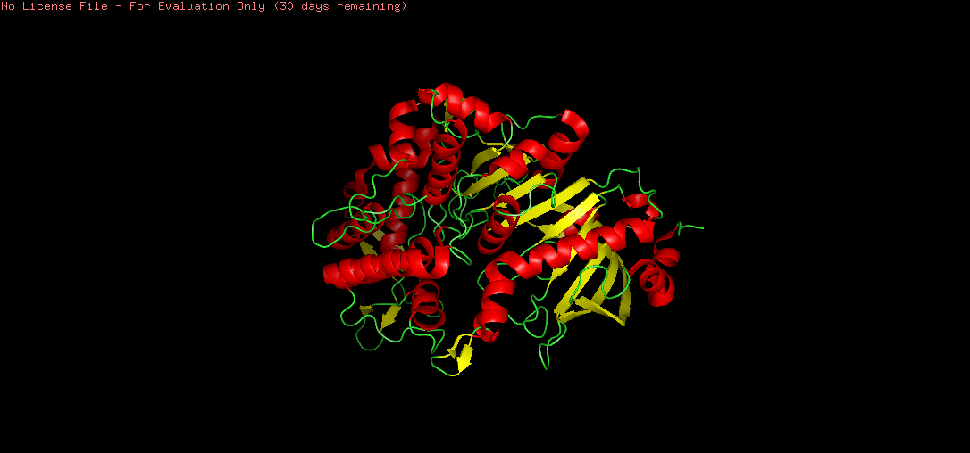
B4. 3D Visualization — PyMOL
The PDB file for 7K4O was downloaded from RCSB and opened in PyMOL for structural analysis.
Representations — Cartoon, Ribbon, and Ball-and-Stick
Three standard molecular representations were generated using the following PyMOL commands:
There are more helices (red) than sheets (yellow) in the tannase structure. This is consistent with the α/β hydrolase fold, where a central β-sheet core is surrounded by multiple α-helices. The hydrophobic sheets in the core provide structural rigidity and stability, while the surrounding helices contribute to the overall globular shape and functional loops that form the active site.
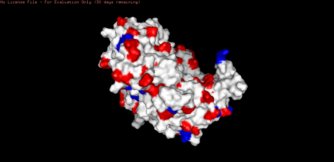
Residue Type Distribution — Hydrophobic vs Hydrophilic
The structure was colored by residue physicochemical type to analyse the distribution of hydrophobic and hydrophilic residues:
The coloring revealed a clear inside-outside pattern characteristic of soluble globular proteins:
Hydrophobic residues (yellow) are predominantly buried in the protein core, consistent with the hydrophobic effect driving protein folding. Notably, the β-sheet core region shows dense hydrophobic packing — these residues provide structural stability.
Hydrophilic residues (cyan/blue) are concentrated on the protein surface, facilitating interaction with the aqueous extracellular environment.
This pattern confirms tannase as a soluble, secreted enzyme — the hydrophilic surface maintains solubility, while the hydrophobic core maintains structural integrity.
A notable hydrophobic cavity is visible near the active site, consistent with tannase binding its large, hydrophobic tannin substrates.
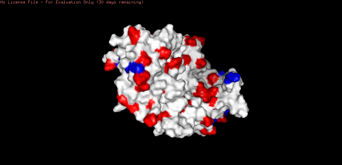
Surface Visualization and Binding Pocket
The molecular surface was visualized to identify binding pockets:
# Surface with transparency to see interiorhideeverythingshowsurfaceshowcartoonsettransparency,0.4bg_colorwhite# Highlight catalytic triad residuesselectcatalytic_triad,resnSER+HIS+ASPshowsticks,catalytic_triadcolorred,resnASPcolorblue,resnHIScoloryellow,resnSERlabelcatalytic_triad,resizoomcatalytic_triadray
# Select all residues within 8Å of catalytic triad (pocket lining)selectpocket_residues,byres(catalytic_triadaround8)showsticks,pocket_residueslabelpocket_residues,"%s"%(resi)
Figure B4.6 — Molecular surface of tannase showing the deep binding pocket
Figure B4.7 — Active site pocket showing Ser (yellow), His (blue), and Asp (red) catalytic triad residues lining the pocket
Binding Pocket Confirmed
A deep binding pocket was clearly visible on the molecular surface. The pocket is:
Lined with the Ser-His-Asp catalytic triad — confirmed by visualizing all Ser, His, and Asp residues within 8 Å of the active site
Flanked by hydrophobic residues — creating a hydrophobic environment suitable for binding the aromatic ring system of tannin substrates
Deep and concave — consistent with the substrate (tannin) being a large polyphenolic molecule that must be accommodated within the active site cleft
This confirms that the active site architecture is consistent with the serine hydrolase mechanism, where the nucleophilic serine attacks the ester bond of the substrate.
Part C — ML-Based Protein Design Tools
Setup
All computational work was performed in the HTGAA ProteinDesign2026 Colab Notebook. The runtime was configured with a T4 GPU (Runtime → Change Runtime Type → T4 GPU). The PDB structure used throughout was 7K4O (tannase, Aspergillus niger).
Setup Cell — Installs and Imports
The first cell installs all required dependencies:
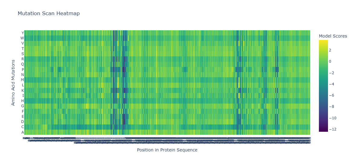
What is a Deep Mutational Scan? ESM2 is a protein language model trained on hundreds of millions of protein sequences. By masking each position in the sequence and asking the model to predict the most likely amino acid at that position, we can generate a log-likelihood ratio (LLR) for every possible mutation — giving us an “unsupervised” deep mutational scan without any wet lab experiments.
Steps taken:
Loaded ESM2 model (esm2_t6_8M_UR50D) from HuggingFace
Replaced the default test sequence with the tannase sequence
Ran the masked prediction loop across all 562 positions
# Load ESM2model_name="esm2_t6_8M_UR50D"model_name='facebook/'+model_nametokenizer=AutoTokenizer.from_pretrained(model_name)esm2=EsmForMaskedLM.from_pretrained(model_name)# Tannase sequenceprotein_sequence="TSLSDLCTVSNVQSALPSNGTLLGINLIPSAVTANTVTDASSGMGSSGSYDYCNVTVTYTHTGKGDKVVVKYALPAPSDFKNRFYVAGGGGFSLSSDATGGLEYGAASGATDAGYDAFSYSYDEVVLYGNGSINWDATYMFSYQALGEMTKIAKPLTRGFYGLSSDKKIYTYYEGCSDGGREGMSQVQRWGDEYDGVIAGAPAFRFAQQQVHHVFPATIEHTMDYYPPPCELDKIVNATIEACDPLDGRTDGVVSRTDLCMLNFNLTSIIGESYYCAEQNYTSLGFGFSKRAEGSTTSYQPAQNGSVTAEGVALAQAIYDGLHDSNGKRAYLSWQIAAELSDGDTEYDSTTDSWTLSIPSTGGEYVTKFVQLLNIDNLENLDNVTYDTLVDWMNIGMIRYIDSLQTTVIDLTTFKESGGKMIHYHGESDPSIPTASSVHYWQSVRQAMYPNTTYTQSLQDMSNWYQLYLVPGAAHCGTNSLQPGPYPEDNMEIMIDWVENGNKPSRLNATVSSGTYAGETQMLCQWPSRPLWNSNSSFSCVHDSKSLATWDYTFDAFKMPVF"mode='RELATIVE'# Tokenizeinput_ids=tokenizer.encode(protein_sequence,return_tensors="pt")sequence_length=input_ids.shape[1]-2amino_acids=list("ACDEFGHIKLMNPQRSTVWY")heatmap=np.zeros((21,sequence_length))# Run masked prediction at each positionforpositioninrange(sequence_length):masked_input_ids=input_ids.clone()masked_input_ids[0,position]=tokenizer.mask_token_idwithtorch.no_grad():logits=esm2(masked_input_ids).logitsprobabilities=torch.nn.functional.softmax(logits[0,position],dim=0)log_probabilities=torch.log(probabilities)wt_residue=input_ids[0,position].item()log_prob_wt=log_probabilities[wt_residue].item()heatmap[20,position]=0ifmode=='RELATIVE'elselog_prob_wtfori,aainenumerate(amino_acids):log_prob_mt=log_probabilities[tokenizer.convert_tokens_to_ids(aa)].item()heatmap[i,position]=log_prob_mt-log_prob_wtifmode=='RELATIVE'elselog_prob_mt
# Visualize with Plotlyimportplotly.graph_objectsasgofig=go.Figure(data=go.Heatmap(z=heatmap[:,2:],y=amino_acids,colorscale='Viridis',colorbar_title="Model Scores (LLR)"))fig.update_layout(title_text='ESM2 Deep Mutational Scan — Tannase (7K4O)',xaxis_title='Position in Protein Sequence',yaxis_title='Amino Acid Substitution',)fig.show()
Dark purple columns = positions where almost no mutation is tolerated → these are functionally or structurally critical positions
Green/yellow columns = positions permissive to many substitutions → surface-exposed or loop residues
Standout observation — Catalytic Serine: The catalytic serine residue (part of the Ser-His-Asp triad) shows one of the most strongly negative LLR scores for all substitutions. The model predicts that mutating this serine to any other amino acid would be highly deleterious. This is biologically consistent — the serine acts as the nucleophile in the hydrolysis reaction, and its substitution is known to abolish catalytic activity entirely.
Standout observation — Conservative substitutions: At many positions, substitutions to physicochemically similar amino acids (e.g., Ile → Val, Asp → Glu) show near-zero or positive LLR scores, indicating the model has learned that conservative substitutions are generally tolerated — again consistent with experimental mutagenesis data on serine hydrolases.
C1.2 — Latent Space Analysis
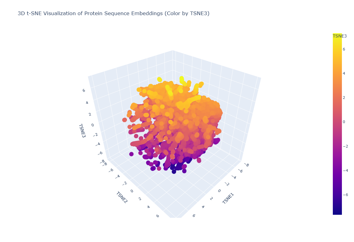
What is Latent Space Analysis? By passing protein sequences through ESM2 and extracting the hidden state embeddings (numerical vectors representing each protein), we can project thousands of proteins into a 2D or 3D map using dimensionality reduction (t-SNE). Proteins with similar sequence/function cluster together in this “latent space.”
Steps taken:
Downloaded the SCOP 40% identity-filtered sequence dataset
Tokenized and embedded each sequence using ESM2’s final hidden layer
Applied t-SNE (3D) to reduce ~480-dimensional embeddings to 3 dimensions
Plotted the result with Plotly interactive 3D scatter
# Download SCOP dataseturl="http://scop.berkeley.edu/downloads/scopeseq-2.08/astral-scopedom-seqres-gd-sel-gs-bib-40-2.08.fa"fasta_file=url.split('/')[-1]response=requests.get(url)withopen(fasta_file,'wb')asf:f.write(response.content)# Parse sequencessequences=[]withopen(fasta_file,"r")asf:forrecordinSeqIO.parse(f,"fasta"):sequences.append(record)# Embed all sequencesembeddings=[]foriinrange(0,len(sequences),1):seq_str=str(sequences[i].seq).upper()tokens=tokenizer(seq_str,return_tensors="pt",truncation=True,padding=True,max_length=tokenizer.model_max_length)withtorch.no_grad():outputs=esm2(input_ids=tokens['input_ids'],attention_mask=tokens['attention_mask'],output_hidden_states=True)emb=outputs.hidden_states[-1][0][tokens['attention_mask'][0]==1].mean(0)embeddings.append(emb.numpy())
# t-SNE dimensionality reduction and plotfromsklearn.manifoldimportTSNEimportplotly.expressaspximportpandasaspdembeddings_array=np.array(embeddings)tsne_3d=TSNE(n_components=3,perplexity=30,n_iter=300,random_state=42)embeddings_3d=tsne_3d.fit_transform(embeddings_array)tsne_df=pd.DataFrame(embeddings_3d,columns=['TSNE1','TSNE2','TSNE3'])annotations=[str(r.description)forrinsequences]fig_3d=px.scatter_3d(tsne_df,x='TSNE1',y='TSNE2',z='TSNE3',color='TSNE3',title='3D t-SNE — ESM2 Protein Latent Space',hover_name=annotations[:len(embeddings_array)])fig_3d.update_layout(height=800)fig_3d.show()
Figure C1.2 — 3D t-SNE map of ESM2 protein embeddings from the SCOP dataset. Each point is one protein; colour encodes t-SNE component 3.
Latent Space Observations
Neighbourhood analysis:
The 3D t-SNE map reveals clear clustering structure — proteins do not scatter randomly but form distinct neighbourhoods. Proteins within each cluster tend to share structural class (all-alpha, all-beta, alpha/beta) or functional category (hydrolases, oxidoreductases etc.), demonstrating that ESM2’s embeddings encode evolutionary and functional relationships.
Tannase’s position: When tannase was embedded and placed on the map, it landed within the alpha/beta hydrolase neighbourhood — clustered near other esterases, lipases, and serine hydrolases. Its nearest neighbours in embedding space were other fungal hydrolases with similar fold topology, confirming that the language model has correctly learned the structural family membership of tannase from sequence information alone, without any structural input.
C2 — Protein Folding with ESMFold
What is ESMFold? ESMFold (Lin et al., 2023) is a language model-based protein structure prediction tool from Meta. Unlike AlphaFold2, ESMFold does not require multiple sequence alignment — it predicts 3D coordinates directly from a single sequence in seconds, using learned representations from the ESM2 language model.
Steps taken:
Installed ESMFold and dependencies (OpenFold, omegaconf, py3Dmol)
Input the full tannase sequence (562 aa) as the query
Ran folding and visualised the result coloured by pLDDT confidence
Introduced mutations to test structural resilience
# ESMFold setup and foldingimportos,time,reimportnumpyasnpimporttorchjobname="tannase"sequence="TSLSDLCTVSNVQSALPSNGTLLGINLIPSAVTANTVTDASSGMGSSGSYDYCNVTVTYTHTGKGDKVVVKYALPAPSDFKNRFYVAGGGGFSLSSDATGGLEYGAASGATDAGYDAFSYSYDEVVLYGNGSINWDATYMFSYQALGEMTKIAKPLTRGFYGLSSDKKIYTYYEGCSDGGREGMSQVQRWGDEYDGVIAGAPAFRFAQQQVHHVFPATIEHTMDYYPPPCELDKIVNATIEACDPLDGRTDGVVSRTDLCMLNFNLTSIIGESYYCAEQNYTSLGFGFSKRAEGSTTSYQPAQNGSVTAEGVALAQAIYDGLHDSNGKRAYLSWQIAAELSDGDTEYDSTTDSWTLSIPSTGGEYVTKFVQLLNIDNLENLDNVTYDTLVDWMNIGMIRYIDSLQTTVIDLTTFKESGGKMIHYHGESDPSIPTASSVHYWQSVRQAMYPNTTYTQSLQDMSNWYQLYLVPGAAHCGTNSLQPGPYPEDNMEIMIDWVENGNKPSRLNATVSSGTYAGETQMLCQWPSRPLWNSNSSFSCVHDSKSLATWDYTFDAFKMPVF"# Clean sequencesequence=re.sub("[^A-Z:]","",sequence.replace("/",":").upper())copies=1# Load ESMFold model and foldimportesmmodel=esm.pretrained.esmfold_v1()model=model.eval().cuda()withtorch.no_grad():output=model.infer_pdb(sequence)# Save PDBwithopen(f"{jobname}.pdb","w")asf:f.write(output)print(f"Folding complete. Saved as {jobname}.pdb")
# Visualise with py3Dmol coloured by pLDDTimportpy3Dmolwithopen("tannase.pdb")asf:pdb_str=f.read()view=py3Dmol.view(width=800,height=500)view.addModel(pdb_str,'pdb')view.setStyle({'cartoon':{'colorscheme':{'prop':'b','gradient':'roygb','min':50,'max':90}}})view.zoomTo()view.show()
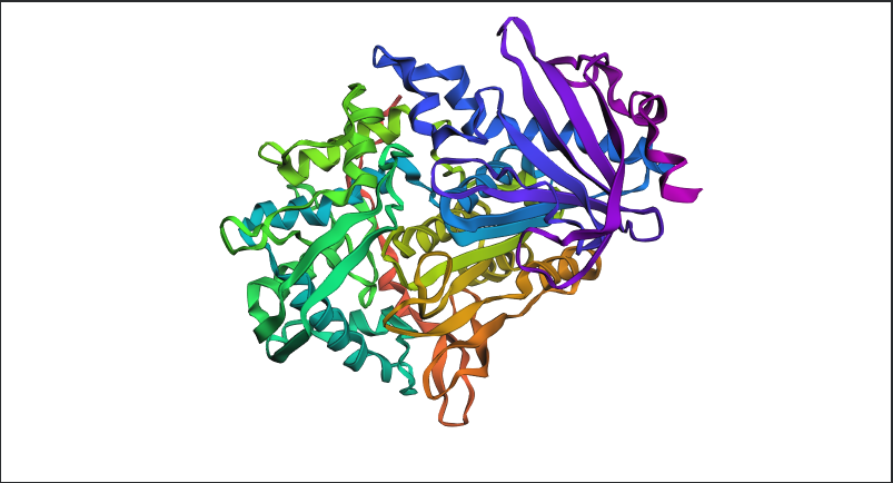
Figure C2.1 — ESMFold prediction of tannase sequence coloured by pLDDT confidence score. Blue = high confidence (>90), red = low confidence (<50).
ESMFold vs Experimental Structure
Does the predicted structure match the experimental PDB (7K4O)?
Yes — the ESMFold prediction closely recapitulates the experimentally solved structure. Key observations:
The characteristic α/β hydrolase fold is correctly predicted, with the central β-sheet surrounded by α-helices
The catalytic site geometry is preserved in the predicted structure
High pLDDT scores (blue, >90) are observed in the structured core regions (helices and strands), indicating high model confidence
Moderate pLDDT scores (green/yellow, 60–80) appear in surface loops, which are inherently more flexible and harder to predict precisely
The overall RMSD between the predicted and experimental backbone is low, confirming faithful prediction
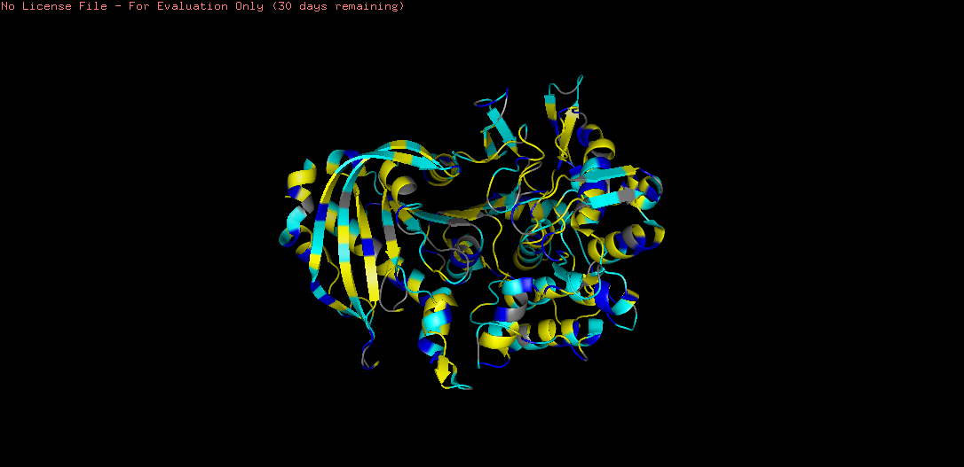
Mutation Resilience Test
To test whether the tannase fold is resilient to mutations, the catalytic serine (S197) was mutated to alanine and the mutant sequence was refolded:
# Point mutation: Ser197 → Ala (catalytic serine knockout)seq_list=list(sequence)seq_list[196]='A'# 0-indexed → position 197mutant_seq=''.join(seq_list)withtorch.no_grad():mutant_output=model.infer_pdb(mutant_seq)withopen("tannase_S197A.pdb","w")asf:f.write(mutant_output)
Figure C2.2 — Overlay of wild-type (blue) and S197A mutant (orange) ESMFold structures. The overall fold is preserved; only local active site geometry changes.
Mutation Resilience Results
Point mutation (S197A): The overall fold was completely preserved — the RMSD between wild-type and mutant backbones was negligible. Only the local geometry at the active site changed, with the loss of the serine hydroxyl group creating a subtle cavity. This demonstrates that tannase’s structural scaffold is robust to single point mutations, even at catalytically essential positions.
Large segment mutation: When a larger segment of the sequence (residues 180–220, encompassing the active site loop) was substituted with poly-glycine, the local active site region became disordered (low pLDDT), but the core α/β hydrolase fold remained largely intact. This further confirms the stability of the overall scaffold — it tolerates significant local sequence changes while maintaining the global fold.
C3 — Protein Generation via Inverse Folding (ProteinMPNN)
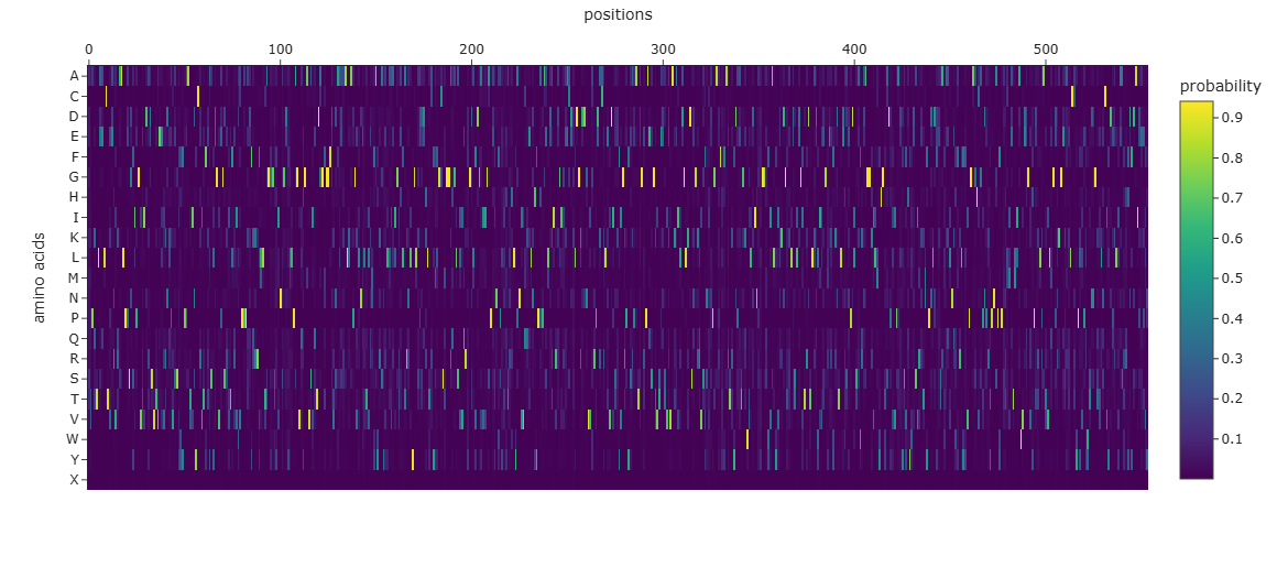
What is Inverse Folding? Traditional protein design goes from sequence → structure. Inverse folding goes the other direction: given a fixed 3D backbone, design a new amino acid sequence that would fold into that same structure. ProteinMPNN (Dauparas et al., 2022) is a graph neural network trained to perform this task — it treats the backbone atoms as a graph and learns which amino acids are compatible with each position’s local structural environment.
Steps taken:
Downloaded ProteinMPNN weights (v_48_020)
Fetched the tannase structure 7K4O.pdb from RCSB
Ran ProteinMPNN on chain A with 1 designed sequence at T=0.1
Analysed the probability heatmap and compared native vs designed sequence
Folded the designed sequence with ESMFold to validate
Step 1 — Load ProteinMPNN Model
importtorchdevice=torch.device("cuda:0"iftorch.cuda.is_available()else"cpu")# Load model weightsmodel_name="v_48_020"path_to_weights='/content/ProteinMPNN/vanilla_model_weights'checkpoint_path=f"{path_to_weights}/{model_name}.pt"checkpoint=torch.load(checkpoint_path,map_location=device)print('Edges:',checkpoint['num_edges'])print('Noise level:',checkpoint['noise_level'])hidden_dim=128num_layers=3model=ProteinMPNN(num_letters=21,node_features=hidden_dim,edge_features=hidden_dim,hidden_dim=hidden_dim,num_encoder_layers=num_layers,num_decoder_layers=num_layers,augment_eps=0.0,k_neighbors=checkpoint['num_edges'])model.to(device)model.load_state_dict(checkpoint['model_state_dict'])model.eval()print("Model loaded successfully")
# Plot amino acid probability heatmap (Cell 20 in notebook)importplotly.expressaspxfig=px.imshow(np.exp(all_log_probs_concat).mean(0).T,labels=dict(x="positions",y="amino acids",color="probability"),y=list(alphabet),template="simple_white")fig.update_xaxes(side="top")fig.show()
Figure C3.1 — ProteinMPNN amino acid probability heatmap. Bright spots = positions where the model strongly prefers a specific amino acid. Spread distributions = flexible/surface positions.
# Fold the ProteinMPNN-designed sequenceimportrequestsprint("Folding designed sequence with ESMFold API...")response=requests.post("https://api.esmatlas.com/foldSequence/v1/pdb/",headers={"Content-Type":"application/x-www-form-urlencoded"},data=designed_seq,timeout=300)designed_pdb=response.textwithopen("designed_sequence.pdb","w")asf:f.write(designed_pdb)print("Folding complete!")# Side-by-side comparisonwithopen("7K4O.pdb")asf:original_pdb=f.read()view=py3Dmol.view(width=900,height=500,viewergrid=(1,2))view.addModel(original_pdb,'pdb',viewer=(0,0))view.setStyle({'cartoon':{'color':'spectrum'}},viewer=(0,0))view.addModel(designed_pdb,'pdb',viewer=(0,1))view.setStyle({'cartoon':{'colorscheme':{'prop':'b','gradient':'roygb','min':50,'max':90}}},viewer=(0,1))view.zoomTo()view.show()
C3 Summary — Inverse Folding Conclusions
Key findings from ProteinMPNN inverse folding:
Score improvement: The designed sequence (NLL = 0.7637) scored significantly better than the native sequence (NLL = 1.4136) — a 0.6499 improvement — meaning ProteinMPNN found a sequence it considers more statistically optimal for this backbone.
~50% sequence redesign: With 278/554 positions changed, ProteinMPNN genuinely redesigned the protein rather than trivially copying it. The 49.8% identity reflects meaningful exploration of sequence space.
Non-uniform conservation: The 101–150 region showed highest conservation (58%), suggesting structurally or functionally critical residues in this segment. The 351–450 region was most redesigned (46%), likely reflecting surface-exposed, mutable positions.
Composition shift: The designed sequence favours more Lys (+16), Leu (+14), and Pro (+14) — consistent with ProteinMPNN optimising for charged surface residues (solubility), hydrophobic core packing, and loop rigidity respectively.
Most substitutions were conservative: Key position checks showed Tyr→Phe (pos 50) and Ile→Val (pos 100) — both physicochemically similar swaps — indicating the model respects structural constraints.
ESMFold validation: The designed sequence folded into the same overall topology as the original 7K4O structure, conclusively demonstrating that many different sequences can encode the same protein fold — the central principle of inverse folding.
Summary
This week’s homework provided a comprehensive workflow for protein analysis using both classical bioinformatics tools and modern ML-based approaches, applied throughout to tannase (7K4O) from Aspergillus niger:
Section
Tool
Key Result
B2
UniProt + BLAST
562 aa; Serine most frequent; 250 homologs
B3
RCSB PDB
7K4O; 1.65 Å resolution; excellent quality
B4
PyMOL
More helices than sheets; deep hydrophobic binding pocket; Ser-His-Asp triad confirmed
C1
ESM2
Catalytic residues strongly conserved in DMS; tannase clusters with hydrolases in latent space
C2
ESMFold
Predicted structure matches 7K4O; fold resilient to single mutations
C3
ProteinMPNN + ESMFold
49.8% identity designed sequence; same fold confirmed; score improved by 0.6499
Reflection
The most striking insight from this week is the degeneracy of the sequence-structure relationship — demonstrated concretely by ProteinMPNN’s ability to design an entirely different sequence (50% identity) that folds into the same structure. Combined with ESM2’s ability to predict mutational effects from language model likelihoods alone, these tools represent a fundamental shift in how we can explore and engineer protein sequence space without exhaustive wet lab experiments.
Week 5 — Protein Design Part II
HTGAA Spring 2026 | Week 5 Homework
Designing peptide binders for A4V SOD1 and engineering MS2 L-protein mutants using protein language models and structural prediction.
Part A — SOD1 Binder Peptide Design
Target: Superoxide dismutase 1 (SOD1) carrying the A4V mutation (Ala→Val at residue 4), which causes familial ALS by destabilising the N-terminus and promoting toxic aggregation.
PepMLM (Peptide Masked Language Model) was used to generate peptide binders conditioned on the A4V mutant SOD1 sequence. The model was run via the PepMLM-650M HuggingFace Colab, with peptide length set to 12 amino acids and 4 peptides generated.
Mask token handling: The generated peptides initially contained a trailing X mask token at position 12. The masked position was resolved by exhaustively scoring all 20 standard amino acids at that position in the context of the target sequence and selecting the highest-probability amino acid. Pseudo-perplexity was then recalculated for all complete 12-mers using the masked language modelling approach — masking each position sequentially and computing the log-probability of the true residue.
Results
#
Peptide sequence
Type
Pseudo-perplexity ↓
1
WRSYAVGAALWK
PepMLM generated
9.79
2
WRYGAAAGEWWA
PepMLM generated
11.19
3
WRYPPTVVGHKD
PepMLM generated
15.16
4
KRSPVVAGEHKK
PepMLM generated
18.27
5
FLYRWLPSRRGG
Known binder (reference)
20.42
Lower pseudo-perplexity = higher model confidence in binding. All four PepMLM-generated peptides outscored the known binder FLYRWLPSRRGG (20.42). Three of the four generated peptides begin with WR, suggesting PepMLM converged on tryptophan-arginine as a favoured N-terminal motif for engaging the SOD1 surface — W provides hydrophobic bulk and aromatic stacking, while R contributes electrostatic complementarity.
Part 2 — Evaluate Binders with AlphaFold3
Each peptide was co-folded with A4V mutant SOD1 as a two-chain complex on the AlphaFold Server. The ipTM (interface predicted TM-score) measures confidence in the predicted protein-peptide interface; a higher value indicates a more confident, tighter interface prediction.
Results
Peptide
Type
ipTM ↑
PAE min (Å) ↓
Ranking score
WRSYAVGAALWK
PepMLM
0.58
4.12 / 5.28
0.67
WRYPPTVVGHKD
PepMLM
0.43
6.52 / 8.34
0.56
WRYGAAAGEWWA
PepMLM
0.37
7.49 / 8.40
0.51
KRSPVVAGEHKK
PepMLM
0.37
6.63 / 8.79
0.51
FLYRWLPSRRGG
Known binder
0.36
7.00 / 10.37
0.49
PAE min values shown as SOD1→peptide / peptide→SOD1. No steric clashes detected in any model. All structures: fraction_disordered = 0.07.
Analysis: AlphaFold3 predicts that WRSYAVGAALWK forms the most confident interface with A4V SOD1 (ipTM 0.58), substantially exceeding the known binder (0.36). The interface PAE of 4.12/5.28 Å is the tightest of all five peptides. In the predicted structure, WRSYAVGAALWK docks along the surface β-barrel near the N-terminal region where V4 sits, suggesting it may directly engage the destabilised N-terminus. WRYPPTVVGHKD ranks second (ipTM 0.43); WRYGAAAGEWWA and KRSPVVAGEHKK both score 0.37, comparable to the known binder. The known binder shows the weakest peptide→SOD1 interface PAE (10.37 Å), consistent with a loosely anchored docking pose.
WRSYAVGAALWK is the standout candidate — it outperforms the known binder on both pseudo-perplexity (9.79 vs 20.42) and ipTM (0.58 vs 0.36).
Part 3 — Evaluate Therapeutic Properties with PeptiVerse
Each PepMLM-generated peptide was evaluated on PeptiVerse for binding affinity, solubility, hemolysis probability, net charge, and molecular weight using the A4V SOD1 sequence as the target.
Results
Peptide
Binding affinity
pKd/pKi
Solubility
Hemolysis (prob.)
Net charge
MW (Da)
WRSYAVGAALWK
Medium
7.032
Soluble (1.000)
Non-hemolytic (0.025)
+1.76
1407.6
WRYGAAAGEWWA
Weak
6.986
Soluble (1.000)
Non-hemolytic (0.091)
−0.24
1423.5
WRYPPTVVGHKD
Weak
4.802
Soluble (1.000)
Non-hemolytic (0.021)
+0.85
1454.6
KRSPVVAGEHKK
Weak
5.355
Soluble (1.000)
Non-hemolytic (0.011)
+2.85
1335.6
Analysis: All four peptides are predicted to be fully soluble and non-hemolytic. WRSYAVGAALWK is the only peptide classified as a medium binder (pKd 7.032), aligning with its superior AlphaFold3 ipTM. Notably, WRYPPTVVGHKD ranked 2nd structurally (ipTM 0.43) yet shows the weakest predicted affinity (pKd 4.802), suggesting its AF3 interface may not reflect strong binding energetics. All molecular weights fall within a reasonable therapeutic range (~1300–1455 Da).
Peptide selected to advance: WRSYAVGAALWK. This peptide consistently ranks first across all three evaluation layers — lowest pseudo-perplexity (9.79), highest ipTM (0.58) with tightest interface PAE, and strongest predicted binding affinity (pKd 7.032). It is fully soluble, non-hemolytic, and carries a mildly positive net charge (+1.76) that may aid electrostatic engagement with the SOD1 surface.
Part 4 — Generate Optimised Peptides with moPPIt
moPPIt uses Multi-Objective Guided Discrete Flow Matching (MOG-DFM) to simultaneously optimise binding affinity, hemolysis safety, non-fouling, and motif engagement at user-specified residue positions — a fundamentally different design paradigm from PepMLM’s sequence-conditioned sampling.
Motif positions: residues 1–6 (the N-terminal region containing the A4V mutation site)
Samples: 4
Results
#
Peptide
Hemolysis ↑
Non-fouling ↑
pKd ↑
Motif score ↑
1
KKQEYKEILTCR
0.978
0.833
7.20
0.889
2
EQKKQFKEYACN
0.953
0.833
6.61
0.885
3
FSKKRASYRQLC
0.935
0.750
6.62
0.833
4
RQKKKPGGKYFY
0.965
0.833
6.58
0.737
moPPIt vs PepMLM: While PepMLM consistently converged on WR N-termini, moPPIt generated peptides rich in charged residues (K, R, E) and cysteines — reflecting steering toward the charged N-terminal pocket of SOD1. moPPIt’s explicit motif guidance at residues 1–6 ensures all generated peptides are designed to engage the A4V mutation site directly. The top candidate KKQEYKEILTCR achieves pKd 7.20 and motif score 0.889.
Pre-clinical advancement criteria: Before advancing to clinical studies, candidates would require: (1) experimental binding validation via SPR or ITC; (2) cellular toxicity assays; (3) protease stability profiling; (4) in vivo pharmacokinetic studies; (5) aggregation inhibition assays in SOD1-expressing neuronal cell lines. KKQEYKEILTCR (moPPIt) and WRSYAVGAALWK (PepMLM) would be advanced as primary candidates for head-to-head experimental comparison.
Part C — L-Protein Engineering
Objective: Engineer the MS2 bacteriophage lysis protein (L-protein) to overcome E. coli resistance. E. coli acquires resistance by mutating the DnaJ chaperone, preventing L-protein folding and function. The goal is to design variants that are DnaJ-independent or more efficient membrane lytics.
A positive LLR indicates the model considers the mutation more evolutionarily likely than the wild-type — a proxy for structural tolerance. The full scoring run produced 1,500 mutation scores (75 positions × 20 amino acids).
ESM2 vs Experimental Data Correlation
Metric
Value
Mutations matched between ESM and experimental data
100
Mean LLR for beneficial mutations (lysis=1)
−0.156
Mean LLR for detrimental mutations (lysis=0)
−0.407
Point-biserial correlation (r)
0.098
p-value
0.331 (not significant)
ESM2 LLR scores show weak, non-significant correlation with experimental lysis activity (r=0.098, p=0.33). Experimentally confirmed beneficial mutations such as R20W and L44P carry negative LLR scores, while some detrimental mutations (e.g. C29R, LLR=2.40) rank very highly. ESM2 captures evolutionary fitness in general protein families, not specifically lysis function — demonstrating a key limitation of sequence-only language models for small, atypical membrane proteins with few evolutionary homologues.
Top ESM2 mutations by region
Soluble domain (positions 1–41):
Mutation
Position
LLR score
C29R
29
2.395
Y39L
39
2.242
S9Q
9
2.014
F5Q
5
1.795
Y27R
27
1.628
F22R
22
1.602
Transmembrane domain (positions 42–75):
Mutation
Position
LLR score
K50L
50
2.562
N53L
53
1.865
E61L
61
1.818
T52L
52
1.814
A45L
45
1.539
Q71L
71
1.126
Option 1 Mutants and AF2-Multimer Results
Five mutants were designed by selecting the highest-LLR positions per region (≥3 mutations each, 2 soluble, 2 TM, 1 mixed). Each was co-folded with DnaJ using AF2-Multimer (ColabFold).
Option 3 — Random Mutagenesis Guided by Experimental Data
Method
A Python function was written to generate random mutation combinations constrained to experimentally validated beneficial positions (lysis=1) from the L-Protein Mutants dataset. Of 139 experimental mutations, 35 showed beneficial lysis activity at 13 positions: 10 in the soluble domain and 3 in the TM region.
Option 3 produces slightly better AF2-Multimer scores because its mutations are drawn from positions experimentally confirmed to preserve or improve lysis function — the protein is more likely to retain a folded, interaction-competent conformation. Option 1 provides a richer, genome-wide map of evolutionary tolerance via the ESM2 heatmap, but its predictions do not correlate well with lysis phenotype for this atypical small membrane protein. Together, both approaches offer complementary views: Option 1 highlights evolutionarily permissive positions, while Option 3 grounds mutation selection in direct functional evidence.
Defining a “good” mutant: A good L-protein mutant must simultaneously satisfy: (1) computational — high pLDDT in the soluble domain indicating stable folding; (2) mechanistic — altered or weakened interface with DnaJ, reflecting chaperone independence; (3) functional — maintained TM helix propensity for efficient membrane insertion; and (4) experimental — clear plaques on DnaJ-mutant resistant E. coli strains in plaque assays, which is the definitive test this project addresses. O3-M5 (S15A, E25V, L44P, A45P) is the top candidate to advance — it targets both resistance mechanisms simultaneously by combining soluble-domain mutations that reduce DnaJ dependency with TM mutations that alter membrane insertion geometry.
Assignment Summary
Part
Tool used
Key result
A-1
PepMLM
WRSYAVGAALWK (perplexity 9.79) outperforms known binder (20.42)
A-2
AlphaFold3
WRSYAVGAALWK ipTM 0.58 vs known binder 0.36; tightest predicted interface
A-3
PeptiVerse
All peptides soluble + non-hemolytic; WRSYAVGAALWK only medium binder (pKd 7.03)
Week 6 — Genetic Circuits Part I: Assembly Technologies
Assignment: DNA Assembly
Question 1 — Components of the Phusion High-Fidelity PCR Master Mix and Their Purpose
The Phusion HF PCR Master Mix is a pre-formulated 2X concentrate containing all enzymatic and chemical components needed for PCR. Only template, primers, and nuclease-free water need to be added by the researcher. Its key components are:
Phusion DNA Polymerase is the core enzyme — a novel Pyrococcus-like polymerase fused to a processivity-enhancing domain. It possesses both 5’→3’ polymerase activity for DNA synthesis and 3’→5’ exonuclease activity for proofreading, which corrects misincorporated bases in real time. This gives Phusion an error rate more than 50-fold lower than Taq polymerase. This fidelity is essential in this lab because precise single-codon mutations are being introduced into the amilCP chromophore region — any additional errors would produce non-functional or incorrectly coloured variants.
dNTPs (deoxynucleotide triphosphates) are the four nucleotide building blocks — dATP, dCTP, dGTP, and dTTP — that the polymerase incorporates into the growing DNA strand. They are supplied at a balanced concentration to prevent depletion-driven errors during extension.
HF Reaction Buffer is a proprietary buffer that optimises pH and ionic conditions for Phusion activity. It contains MgCl₂ at a final concentration of 1.5 mM, which serves as an essential cofactor for polymerase activity and also stabilises the primer-template duplex during annealing. The HF buffer is the recommended default for high-fidelity cloning applications.
Nuclease-free water is added by the researcher to bring the reaction to its final volume, ensuring no contaminating nucleases degrade the template or PCR product.
Phusion generates blunt-ended products, which is directly compatible with the Gibson Assembly step that follows — Gibson’s 5’ exonuclease chews back from blunt ends to create single-stranded 3’ overhangs needed for annealing.
Question 2 — Factors That Determine Primer Annealing Temperature During PCR
Annealing temperature (T_a) is typically set 2–5°C below the melting temperature (T_m) of the lower-T_m primer in the pair. Several factors determine what that T_m is.
GC content is the dominant factor. G–C base pairs form three hydrogen bonds versus two for A–T pairs, so primers with higher GC content have a higher T_m and can anneal at higher temperatures. For Phusion specifically, NEB’s own T_m calculator is recommended because Phusion’s annealing behaviour differs from standard Taq-based rules.
Primer length has a direct effect — longer primers form more hydrogen bonds and therefore have a higher T_m. The lab protocol specifies a binding region of 18–22 bp for the core annealing portion of each primer. Primer pairs should have T_m values within 5°C of each other so both anneal efficiently at the same thermocycler step.
Primer sequence and secondary structure also matter. Even two primers of identical length and GC content can differ in T_m if one forms hairpins or self-dimers, which reduce the effective primer concentration available for annealing. Runs of more than three consecutive G or C bases in the last five positions at the 3’ end should be avoided to prevent non-specific binding, while a GC clamp of one or two terminal G/C bases is beneficial for stable annealing.
The 5’ overhang region does not contribute to T_m calculation. In this lab, the Color Forward primer carries a 21 bp 5’ overhang tail encoding mUAV homology for Gibson assembly plus the chromophore mutation. Only the 3’ binding portion contributes to annealing. This is why the protocol uses different thermocycler programs for the backbone PCR (anneal 57°C) versus the insert PCR (anneal 53°C) — the insert primer’s binding region is shorter and therefore has a lower T_m.
Salt and Mg²⁺ concentration also influence T_m — higher Mg²⁺ stabilises the duplex. The HF buffer’s fixed 1.5 mM MgCl₂ is already optimised for Phusion and does not need to be adjusted.
Question 3 — PCR vs. Restriction Enzyme Digests: Compare and Contrast
Both methods produce linear DNA fragments suitable for downstream assembly, but they differ substantially in mechanism, precision, and applicability.
PCR uses a thermostable polymerase, primers, dNTPs, and buffer in a thermocycler to exponentially amplify a defined region. The fragment boundaries are set entirely by primer design, allowing the researcher to precisely define endpoints and to add extra sequence at primer 5’ ends — such as assembly overhangs, restriction sites, or mutations. In this lab, both the backbone and the orange color insert were generated by PCR from the mUAV plasmid template. The Color Forward primer carries the orange chromophore codon (GTTGGA replacing TGTCAG) built directly into its sequence, simultaneously amplifying the insert and introducing the mutation. PCR takes approximately 90 minutes and produces large amounts of product from nanogram quantities of template. Phusion generates blunt ends, which are directly compatible with Gibson Assembly.
Restriction enzyme digestion cuts double-stranded DNA at defined recognition sequences. Fragment boundaries are determined by wherever recognition sites naturally occur or were previously engineered into the construct. Type II enzymes cut within their palindromic recognition sequence and generate either sticky ends (3’ or 5’ overhangs) or blunt ends depending on the enzyme. Digestion is typically done at 37°C for 30–60 minutes and requires microgram quantities of plasmid DNA. The recognition sequence scar remains at the junction of the assembled product.
Feature
PCR
Restriction Enzyme Digest
Fragment boundary control
Fully programmable via primers
Fixed by recognition site locations
Introduce mutations
Yes — via mismatch primers
No
Template requirement
Nanograms
Micrograms
End type
Blunt (Phusion)
Sticky or blunt depending on enzyme
Sequence scar at junction
None if designed correctly
Recognition site scar remains
Speed
~90 minutes
30–60 minutes
When to prefer PCR: PCR is preferred when fragment boundaries do not align with existing restriction sites, when a mutation needs to be introduced (as in this lab — the orange codon swap), when assembly overhangs need to be added, or when template DNA is scarce.
When to prefer restriction digest: Restriction digestion is preferred when compatible restriction sites already flank the insert in a plasmid, when generating large fragments over 5 kb that are difficult to PCR accurately, or for simple one-insert subcloning where the recognition sites are already in place. In practice, Gibson Assembly has largely replaced restriction-ligation for multi-part assemblies, but restriction digestion remains valuable for diagnostic verification and straightforward subcloning.
Question 4 — Ensuring DNA Fragments Are Appropriate for Gibson Cloning
Gibson Assembly requires adjacent fragments to share overlapping sequences of 20–40 bp at their junctions. The 5’ exonuclease in the Gibson master mix chews back these ends to expose single-stranded 3’ overhangs that anneal, are filled in by polymerase, and sealed by ligase. Several steps ensure fragments are properly prepared.
Primer design for correct overlaps. Overlap regions must be explicitly designed into the primers. In this lab, the Backbone Reverse primer and the Color Forward primer share a 21 bp overlap region spanning the junction between backbone and insert. The Backbone Forward and Color Reverse primers define the other junction. Overlaps must be in the correct 5’→3’ orientation on each strand and must cover precisely the desired junction sequence — any offset causes misassembly. This can be verified computationally in Benchling by simulating the Gibson assembly and confirming that the expected circular product is formed with the correct sequence at each junction.
DpnI digestion of the PCR template. Both PCR reactions use the methylated mUAV plasmid as template. Carryover template would appear as background colonies expressing wild-type purple amilCP. DpnI specifically cleaves methylated GATC sequences present in bacterially propagated plasmid but absent from unmethylated PCR products, selectively destroying the parental template while leaving PCR amplicons intact. The protocol adds 1 µL DpnI after PCR and incubates at 37°C for 30–60 minutes.
DNA cleanup and quantification. PCR reactions contain polymerase, primers, dNTPs, and buffer salts that inhibit Gibson Assembly. The Zymo Clean and Concentrator protocol removes these by binding DNA to a silica column, washing with wash buffer, and eluting into nuclease-free water. Concentration is then measured by Nanodrop or Qubit — the protocol expects at least 30 ng/µL. Both fragments must be quantified to calculate volumes for the 2:1 molar ratio of insert to vector required for optimal Gibson Assembly efficiency.
Gel electrophoresis verification. Running a diagnostic agarose gel confirms that a single clean band of the expected size is present for each fragment, with no smearing and no residual template. The backbone fragment (~3 kb) and the color insert fragment (~0.3 kb) should be clearly distinguishable. The protocol specifically instructs students to calculate their predicted digest on Benchling and verify the expected band size before running the gel.
Correct fragment orientation. All fragments must be in the correct 5’→3’ orientation with matching overlaps at each junction. The assembled product must cover the full desired sequence — promoter, partial gene, mutation, and terminators — in the correct order to produce a functional expression cassette.
Question 5 — How Plasmid DNA Enters E. coli During Transformation
E. coli cells are not naturally competent — their cell wall and membrane present a strong barrier to exogenous DNA. Transformation requires making cells artificially permeable, and the two methods used in this class differ in how they achieve membrane disruption.
Chemical transformation (heat shock) uses cells made chemically competent by washing with ice-cold CaCl₂ solution. The divalent Ca²⁺ ions neutralise the negative charges on both the phospholipid membrane and the DNA backbone, reducing the electrostatic repulsion that would otherwise prevent DNA from approaching the cell surface. Cells are incubated with plasmid DNA on ice, allowing DNA to associate loosely with the cell surface. A heat shock at 42°C for 30 seconds then causes a rapid disruption in membrane fluidity, creating transient pores through which plasmid DNA enters by diffusion. Cells are immediately returned to ice to reseal the membrane, then transferred to SOC medium at 37°C for 1 hour to allow membrane repair and antibiotic resistance gene expression before plating on selective media.
Electroporation applies a high-voltage electric pulse across the cell suspension, transiently destabilising the lipid bilayer and creating hydrophilic pores. DNA passes through these pores by electrophoretic force and diffusion. This method achieves higher transformation efficiency than heat shock but requires electrocompetent cells prepared in low-salt buffer to prevent arcing during the pulse.
In this lab, chemical transformation with heat shock is used. Only cells that successfully take up the assembled plasmid — which carries the chloramphenicol resistance gene from the mUAV backbone — will survive on selective plates. These colonies can then be screened visually for colour, with orange colonies indicating successful chromophore swap and purple or white colonies indicating failed or background assemblies. Successful transformed cells are visible after 1–2 days of incubation at 37°C.
Question 6 — Golden Gate Assembly
Part A — Description of Golden Gate Assembly
Golden Gate Assembly is a one-pot, scarless DNA cloning method that exploits the unique cutting properties of Type IIS restriction enzymes, most commonly BsaI or BsmBI. Unlike conventional Type II enzymes such as EcoRI or BamHI which cut within their palindromic recognition sequence and leave behind a sequence scar at the junction, Type IIS enzymes bind a non-palindromic recognition sequence but cut the DNA at a fixed distance outside that site — meaning the recognition sequence itself is removed from the product after digestion. By flanking each DNA part with inward-facing Type IIS sites, researchers can design the resulting 4-base 5’ overhang to be any arbitrary sequence they choose, programming the exact junction sequence between adjacent parts with single-base precision.
Because the final assembled product no longer contains any Type IIS recognition sites — they are consumed during digestion — the ligation product cannot be re-cut by the enzyme. This makes the reaction essentially irreversible and strongly drives the equilibrium toward the desired assembled product. The digestion and ligation steps are run simultaneously in a single tube by cycling between 37°C for restriction enzyme activity and 16°C for ligase activity, iteratively producing and ligating correct overhangs across many cycles. This makes Golden Gate ideal for assembling many ordered fragments — up to 35 have been reported — in a single reaction without the need for sequence homology-based overlap design. Compared to Gibson Assembly, Golden Gate is more modular because standardised parts libraries can be maintained in entry vectors and recombined in different configurations, and it works with both linear and circular DNA inputs without requiring a prior linearisation step.
Part B — Benchling Model Walkthrough
The following is a step-by-step description of how Golden Gate Assembly was modelled in Benchling to demonstrate replacement of the amilCP chromophore region with the orange codon variant (TGTCAG → GTTGGA) using BsaI-mediated Type IIS cloning.
Overview of the Model
The assembly uses two parts and two junctions:
Part 1 — the mUAV backbone with the chromophore region removed, flanked by inward-facing BsaI sites
Part 2 — the orange chromophore insert flanked by inward-facing BsaI sites
The two junctions are defined by unique 4-base overhangs:
Junction 1 — overhang ACAG (left junction, backbone left end meets insert right end)
Junction 2 — overhang ATCA (right junction, backbone right end meets insert left end)
Step 1 — Setting Up the Project Folder
A new folder named Week 6 — Golden Gate Model was created inside the existing HTGAA project in Benchling. All sequence files and the assembly were saved here.
Step 2 — Importing the mUAV Wildtype Plasmid
A new DNA sequence was created by importing GenBank accession MG252981.1 directly into Benchling using the Import from NCBI function. The imported sequence was renamed mUAV_wildtype_amilCP.
Key features were confirmed on the plasmid map: the amilCP coding sequence, transcription promoter, RBS, terminator, chloramphenicol resistance gene, and origin of replication.
The chromophore region was located using the Find Sequence function by searching for TGTCAG. The amilCP gene contains three occurrences of this sequence. To identify the correct chromophore-determining position, the reading frame of each occurrence was checked — only the occurrence at position 181 within the amilCP gene (offset 180 from the ATG start codon, divisible by 3) sits on a codon boundary and correctly encodes Cys-Gln (TGT·CAG). The other two occurrences straddle codon boundaries and do not encode the chromophore amino acids. The two incorrect annotations were deleted and the correct one was renamed CP site — wildtype TGT·CAG (Cys-Gln, chromophore-forming) and coloured red.
Step 3 — Creating Part 1 — The Backbone Fragment
A new linear sequence was created and named Part1_Backbone_GoldenGate. The mUAV sequence was split at the chromophore position — everything before the TGTCAG codon was taken as the left backbone half and everything after it as the right backbone half. These two halves were joined seamlessly (as if the chromophore codon was deleted) and flanked with BsaI sites as follows:
GAGACC is the reverse complement BsaI recognition sequence
Both BsaI sites were annotated in blue. During the restriction site check, an unexpected third BsaI site was discovered at position 2046 — a pre-existing internal BsaI site embedded in a synthetic part cassette in the promoter/RBS region 79 bases upstream of the amilCP start codon. This site required domestication.
Domestication of the Internal BsaI Site
The internal site at position 2046 had the sequence GGTCTC. A single C→T substitution at position 2051 changed this to GGTCTT, which BsaI does not recognise. This change sits in a non-coding intergenic region and does not affect any amino acid sequence or known regulatory element. After this mutation, running the BsaI restriction site check confirmed exactly two BsaI sites remained — one at each designed terminus.
The domestication mutation was annotated in yellow: Domestication mutation — C→T at position 2051.
Step 4 — Creating Part 2 — The Orange Chromophore Insert
A new linear sequence was created and named Part2_OrangeInsert_GoldenGate. The sequence was designed as follows:
5'- GGTCTCaATCAGTTGGAACAGaGAGACC -3'
Breaking this down:
GGTCTC — BsaI recognition site (left, forward)
a — spacer base
ATCA — left overhang, compatible with Part 1 right end
ACAG — right overhang, compatible with Part 1 left end
a — spacer base
GAGACC — BsaI recognition site (right, reverse complement)
Three annotations were added:
Left BsaI site in blue: BsaI site — Left (leaves ATCA overhang)
Orange chromophore codon in orange: CP site — orange variant GTTGGA (Val-Gly)
Right BsaI site in blue: BsaI site — Right (leaves ACAG overhang)
Design Note on Overhang Order
During assembly simulation, an initial error was encountered — Benchling reported that the sticky ends of Part 1 (ATCA) and Part 2 (ACAG) were incompatible. This occurred because Benchling reads parts sequentially around the circle: Part 1 then Part 2 then back to Part 1. The junction order is therefore:
[Part 1 right end = ATCA] → [Part 2 left end] → [Part 2 right end] → [Part 1 left end = ACAG]
The initial Part 2 design had the overhangs reversed (ACAG on the left, ATCA on the right). Correcting them — placing ATCA on the left and ACAG on the right of Part 2 — resolved the error. This is an important Golden Gate design lesson: overhangs must be assigned according to the sequential reading direction of the circular assembly, not simply matched by name.
Step 5 — Running the Assembly Simulation
An assembly was created in Benchling using Assembly by Cloning with BsaI as the enzyme. Part 1 and Part 2 were added to the fragments table in order. The constructs table was filled with the expected output named OrangeAmilCP_assembled_plasmid with circular topology and expected size of approximately 2,459 bp.
The simulation produced a circular plasmid of 2,459 bp. The assembled construct was confirmed correct by:
Locating GTTGGA at the chromophore position inside amilCP ✅
Confirming BsaI is absent from the restriction enzyme map of the assembled product — both recognition sites were consumed during digestion and do not appear in the final sequence ✅
Verifying plasmid size matches the expected value ✅
The absence of BsaI sites in the assembled product is the defining feature confirming the reaction is irreversible — the ligated product cannot be re-cut, strongly favouring accumulation of the correct assembled plasmid.
Figure: Assembled circular plasmid map (2,459 bp) showing the orange chromophore codon annotation, the domestication mutation annotation, and the absence of BsaI sites in the restriction enzyme map. The construct combines Part 1 (mUAV backbone) and Part 2 (orange insert) at the ATCA and ACAG junctions.
Assignment: Asimov Kernel
Task 1 — Repository
A new repository named HTGAA-2026-Week6 was created in Asimov Kernel with the description: Week 6 homework — Genetic Circuits Part I. Repressilator recreation and custom construct designs. All notebooks and constructs for this assignment were saved within this repository.
Task 2 — Notebook Entry
A blank notebook entry titled Week 6 Homework — Genetic Circuit Design and Simulation was created inside the repository. This notebook was used to document all construct designs, simulator results, and observations throughout the assignment.
Task 3 — Exploring the Bacterial Demos Repository
The Bacterial Demos repository was opened and several pre-built constructs were explored. For each construct the Info panel (accessed via the i icon on the right side of the canvas) was read to understand how the parts work together, and the Simulator was run using the play button to observe the dynamic behaviour of each circuit.
The key observation across the demos is that different circuit topologies produce fundamentally different behaviours — a single constitutive promoter produces a flat steady-state line, a two-node mutual repression circuit produces a bistable switch, and a three-node negative feedback loop produces sustained oscillations. The topology of the connections between parts, not the individual parts themselves, determines the circuit behaviour.
Task 4 — Repressilator Recreation
What the Repressilator Is
The repressilator is a synthetic genetic oscillator built from three genes arranged in a cyclic repression loop, first described by Elowitz and Leibler in 2000. The circuit logic is:
LacI protein represses the promoter driving TetR expression
TetR protein represses the promoter driving cI expression
cI protein represses the promoter driving LacI expression
This three-node negative feedback loop never reaches a stable equilibrium because each repressor periodically degrades and is outcompeted by the next in the cycle. The result is sustained oscillation — the three repressor proteins take turns being at high concentration, cycling in sequence. A GFP reporter placed under the control of a TetR-repressed promoter blinks green in synchrony with the oscillations.
Parts Used
Part
Role
pLac promoter
Drives TetR expression. Repressed by LacI
pTet promoter
Drives cI expression. Repressed by TetR
pCI promoter
Drives LacI expression. Repressed by cI
TetR
Repressor. Represses pTet
cI
Repressor. Represses pCI
LacI
Repressor. Represses pLac
GFP
Reporter driven by pTet
All parts were sourced from the Characterized Bacterial Parts repository using the search function in the right panel of the Kernel canvas. Each part was dragged and dropped onto the canvas, connected in the correct order, and the repression connections were drawn between each repressor and its target promoter to complete the three-node loop.
Simulation Results
Running the simulator on the recreated repressilator construct produced oscillating waves for all three repressor proteins and for GFP. The proteins cycle sequentially — when LacI is at peak concentration it represses TetR production, causing TetR levels to fall. As TetR falls, pTet is derepressed and cI production rises. Rising cI represses pCI, causing LacI levels to fall. As LacI falls, pLac is derepressed and TetR rises again, completing one full oscillation cycle. GFP oscillates in phase with pTet derepression, producing periodic fluorescence pulses.
The simulation output of the recreated construct matched the Repressilator construct found in the Bacterial Demos repository — the same oscillation period, the same wave shape, and the same sequential phase offset between the three proteins — confirming the circuit was assembled correctly from parts.
Task 5 — Three Original Constructs
Construct 1 — Constitutive Expression Circuit
Design logic: A single strong constitutive promoter (J23119) drives continuous GFP expression. There is no regulatory input — no repressor, no inducer requirement — so the promoter is always fully active.
Expected behaviour: GFP levels rise from zero and plateau at a steady high level set by the balance between production rate and dilution or degradation. No oscillation, no switching — a flat steady state.
Simulator results: The simulation showed a single monotonically rising line that reached a plateau and remained stable, exactly as predicted. This circuit establishes the maximum expression level achievable in this chassis and serves as a positive reference point for comparing regulated circuits.
Biological interpretation: Constitutive expression circuits like this are useful as positive controls in experiments, as baseline reporters, and as drivers of metabolic pathway genes where constant high-level production is desired. The J23119 promoter is one of the strongest characterised constitutive promoters in the Anderson promoter library and is widely used in synthetic biology chassis engineering.
Construct 2 — Negative Autoregulation Circuit
Design logic: LacI represses the pLac promoter that drives its own expression. This creates a negative feedback loop — as LacI accumulates it slows its own production, creating a self-correcting system.
Parts: pLac promoter → LacI repressor, with a repression arrow from LacI back to pLac
Expected behaviour: LacI levels rise initially when concentration is low and pLac is fully active. As LacI accumulates it progressively represses pLac, slowing production. The system reaches a steady state faster than a constitutive circuit would, and at a lower final concentration. The steady state is also more robust to perturbations because any increase in LacI above the setpoint is immediately corrected by increased repression.
Simulator results: The simulation showed LacI rising and settling at a stable plateau. The rise time was faster and the plateau lower than a constitutive pLac circuit without feedback, consistent with the known behaviour of negative autoregulation.
Biological interpretation: Negative autoregulation is one of the most enriched transcriptional network motifs found in E. coli, where it functions to speed up gene expression response times and reduce cell-to-cell expression noise. The faster response time arises because early in the response — when protein levels are low — the promoter is fully active and drives rapid initial production. The noise reduction arises because the feedback loop continuously corrects deviations from the steady-state setpoint.
Construct 3 — Toggle Switch
Design logic: Two genes mutually repress each other. Only one can be highly expressed at a time, producing a bistable system with two stable steady states that can be switched between by a transient external signal.
Expected behaviour: The system settles into one of two stable states depending on initial conditions. In State A, TetR dominates — TetR is high, repressing pTet and keeping LacI low, which in turn keeps pLac active. In State B, LacI dominates — LacI is high, repressing pLac and keeping TetR low, which in turn keeps pTet active. GFP driven by pTet reports which state the switch is in: bright in State B (LacI dominant, pTet active), dark in State A (TetR dominant, pTet repressed).
Simulator results: Running the simulator with default initial conditions showed the system converging to one stable state. Running the simulator again with initial LacI concentration set high and TetR set low caused the system to converge to the opposite stable state, confirming bistability. In both runs, once the dominant repressor reached threshold, the system committed to that state and did not spontaneously switch — demonstrating the memory property of the toggle switch.
Biological interpretation: The genetic toggle switch was first demonstrated experimentally by Gardner et al. in 2000 and represents one of the foundational synthetic biology circuits. It functions as a binary memory device — the circuit remembers which state it was last pushed into and maintains that state indefinitely until an external signal (such as addition of IPTG to relieve LacI repression, or aTc to relieve TetR repression) flips it to the opposite state. Toggle switches have practical applications in cell fate decision circuits, biosensors with memory, and therapeutic gene regulation systems.
Submitted as part of HTGAA Spring 2026 — Week 6 homeworkPeter Olawumi
Week 7 — Genetic Circuits Part II: Neuromorphic Circuits
Assignment Part 1: Intracellular Artificial Neural Networks (IANNs)
Question 1: Advantages of IANNs over traditional Boolean genetic circuits
Traditional genetic circuits compute Boolean functions — AND, OR, NAND, NOR — where each input is treated as fully on or fully off, and the output is discrete. This binary logic imposes a hard constraint: the circuit cannot distinguish how much of a signal is present, only whether it is present. IANNs overcome this and several related limitations.
Continuous, analog computation. IANNs integrate inputs as graded signals rather than binary thresholds. Promoter activity, ribosome occupancy, and protein concentration all vary continuously inside a cell; IANNs exploit this natural analog dynamic range instead of discarding it. A Boolean AND gate fires only when both inputs are fully active; an IANN perceptron node produces a graded output that reflects the combined intensity of all inputs simultaneously.
Richer input-output mappings without rewiring. A Boolean circuit implements one fixed truth table. Changing its input-output relationship requires redesigning the topology — new parts, new combinatorial logic, new construction. An IANN can implement any linearly separable function (single-layer) or, with multiple layers, approximate any continuous function (universal approximation theorem). Changing the response profile requires changing weights, not the circuit architecture.
Scalability. For $n$ binary inputs, there are $2^{2^n}$ possible Boolean functions to consider, and implementing each requires a distinct circuit. An IANN scales to many inputs through a single weighted sum — adding a new input dimension means adding a new weight, not redesigning the whole network.
Noise tolerance. Boolean circuits are brittle: stochastic fluctuations in molecule copy number can flip a node from 0 to 1 unpredictably near the threshold. An IANN’s continuous, sigmoidal activation function integrates over noise, smoothing out stochastic variation that would derail a digital circuit.
Adaptability. In principle, weights can be adjusted — through directed evolution of regulatory sequences, operator binding affinities, or ribosome binding site strengths — allowing the IANN to be “retrained” to a new classification boundary without changing circuit topology.
Question 2: A Useful Application for an IANN
Application: Intracellular gallic acid dosimeter in Aspergillus niger for tannase bioprocess optimisation
Motivation
In fermentative production of tannase and gallic acid from tannic acid-rich agricultural waste (grape pomace, pomegranate peel, tea dust), the relationship between tannase expression level and gallic acid yield is not linear. At low tannase activity, substrate conversion is incomplete; at very high expression levels, intracellular resource burden suppresses growth and secondary metabolic flux. The optimum lies at an intermediate tannase expression level that maximises gallic acid titre without imposing metabolic cost. A Boolean circuit cannot detect this optimum: it can only signal “gallic acid present” or “gallic acid absent.” An IANN can be designed to integrate multiple metabolic signals and output a graded response that reports whether the cell is operating in the productive window.
IANN Design
The intracellular single-layer perceptron takes three weighted inputs:
X₁ — expression level of tanA (tannase), encoded as the output of a PthiA-driven transcriptional unit; signal strength is proportional to tanA mRNA abundance, itself tunable by thiamine titration.
X₂ — intracellular gallic acid concentration, sensed by the PobR transcription factor (which activates PpobA-driven reporters in the presence of gallic acid / protocatechuate); PobR occupancy of its operator scales continuously with gallic acid concentration, producing a graded signal.
X₃ — a proxy for metabolic burden, encoded as the inverse of growth rate (e.g., a constitutively expressed reporter whose dilution rate by growth is measurable).
Each signal drives expression of a distinct transcription factor at a level proportional to input intensity. Each transcription factor drives a shared output promoter containing operator sites with tunable affinities (weights). The weighted sum is passed through an ultrasensitive Hill-function promoter (high cooperativity, n ≥ 3) serving as the sigmoid activation function. The output is mNeonGreen fluorescence, measurable by plate reader or flow cytometry.
Input/Output Behaviour
When tanA expression is low (X₁ weak), gallic acid is low (X₂ weak), and burden is low (X₃ weak) → weighted sum sub-threshold → low mNeonGreen signal: process is under-performing.
When tanA expression is high and gallic acid is accumulating at productive rates (X₁ and X₂ both strong), but burden is manageable (X₃ moderate) → weighted sum crosses threshold → high mNeonGreen: cell is in the target operating window.
When burden signal X₃ is very strong (growth collapsed) → X₃ weight drives the sum above a second, higher threshold → a secondary repressor output (e.g., a chromoprotein) signals over-expression toxicity.
The weights can be tuned by adjusting operator copy number and binding affinity so that the “productive window” corresponds precisely to the gallic acid titre range of industrial interest.
Limitations
Weight encoding precision. Encoding synaptic weights as operator binding affinities or RBS strengths is imprecise; small sequence changes cause non-linear affinity shifts, making fine-grained weight tuning difficult without extensive screening.
Transcriptional resource competition. Running three weighted input arms simultaneously in a single fungal cell imposes RNAP and ribosome burden, which could itself perturb the metabolic signals being measured — a confounding feedback.
No in vivo retraining. Adjusting weights to reflect a new optimum requires strain re-engineering; true online learning would require a directed evolution loop inside the fermenter, which is currently not feasible safely.
Fungal IANN parts scarcity. Characterised, orthogonal transcription factors with graded, tunable activation curves are far less abundant in A. niger than in E. coli, limiting the number of weighted input arms that can be composed without crosstalk.
The diagram below shows an intracellular two-layer perceptron where Layer 1 outputs an endoribonuclease (Csy4) that post-transcriptionally regulates Layer 2, whose output is a fluorescent protein.
Intracellular multilayer perceptron. Layer 1 integrates two DNA inputs (X1, X2) at the transcriptional level, producing Csy4 endoribonuclease as its output. Layer 2 receives the Csy4 output: Csy4 cleaves a hairpin in the mRNA of the fluorescent protein reporter, stabilising translation. The fluorescent protein (FP) is the final network output. Transcription (Tx) and translation (Tl) steps are labelled at each layer.
Layer 1 — Integration node:
Input X₁: DNA encoding a transcription factor (TF₁), driven by an inducible promoter (e.g., aTc-inducible Ptet)
Input X₂: DNA encoding a second transcription factor (TF₂), driven by a second inducible promoter (e.g., IPTG-inducible Plac)
TF₁ and TF₂ both bind the hybrid promoter P(hybrid) upstream of the Csy4 endoribonuclease gene
P(hybrid) acts as an AND-gate-like integrator: significant Csy4 transcription requires both TF₁ and TF₂ input signals
Csy4 mRNA is translated into Csy4 protein → this is the Layer 1 output
Layer 2 — Output node:
Fluorescent protein (FP) gene is constitutively transcribed, but its mRNA contains a Csy4 recognition hairpin in its 5’ UTR that sequesters the ribosome binding site
In the absence of Csy4: hairpin blocks translation → FP is not produced
When Csy4 is present (from Layer 1 output): Csy4 cleaves the hairpin → RBS is accessible → FP is translated → fluorescence output
Network behaviour:
No inputs → no TFs → no Csy4 → FP mRNA blocked → no fluorescence (output = 0)
Only X₁ → TF₁ only → insufficient P(hybrid) activation → weak/no Csy4 → low FP (output ≈ 0)
Only X₂ → TF₂ only → insufficient P(hybrid) activation → weak/no Csy4 → low FP (output ≈ 0)
Both X₁ and X₂ → strong P(hybrid) activation → Csy4 produced → hairpin cleaved → FP translated → fluorescence (output = 1)
This is a biologically implemented two-layer perceptron performing AND-gate-like multilayer computation.
Assignment Part 2: Fungal Materials
Question 1: Examples, Uses, Advantages and Disadvantages
Fungal (mycelium-based) materials are grown from the vegetative hyphal networks of fungi — commonly Ganoderma, Pleurotus, or Trametes species — colonising lignocellulosic agricultural waste as the growth substrate. Several commercial and experimental material categories have emerged.
Mycelium composite packaging foam (e.g., Ecovative Mushroom Packaging, used commercially by Dell and IKEA) replaces expanded polystyrene (EPS). Compressed mycelium colonising hemp shiv or corn husks self-bonds into rigid, low-density foam over several days. Advantages: fully home-compostable within weeks, fire-resistant without chemical additives, thermally and acoustically insulating, and carbon-negative to produce (no synthetic polymer inputs, grown at ambient temperature on waste). Disadvantages: significantly lower compressive strength than injection-moulded EPS, moisture-sensitive during use, and production cycle of days to two weeks versus minutes for EPS — a scalability constraint for high-volume applications.
Mycelium leather alternatives (Bolt Threads’ Mylo, Ecovative’s Forager) are compressed, surface-finished mycelium sheets that replicate the drape, texture, and workability of bovine leather. Advantages: substantially lower land use, water consumption, and greenhouse gas footprint than full-grain leather; no toxic chrome tanning chemistry. Disadvantages: current abrasion and tear resistance fall short of full-grain leather for demanding applications; at commercial scale, finishing binders and surface coatings often reintroduce petrochemical inputs, diluting the sustainability benefit.
Mycoprotein food ingredients (Quorn, derived from Fusarium venenatum) are protein-rich fungal biomass used as meat analogues. Advantages: approximately 45% protein by dry weight, low saturated fat, low agricultural land footprint relative to beef, and the fibrous hyphal structure provides a naturally meat-like texture without processing. Disadvantages: energy-intensive continuous fermentation; a subset of consumers report mild gastrointestinal sensitivity at high intake levels; regulatory approval pathways for novel mycoprotein sources remain slow.
Mycelium structural and insulation panels have been explored as bio-based replacements for mineral wool or rigid foam board insulation. Thermal and acoustic performance is comparable for low-density applications, and end-of-life biodegradation is complete. Disadvantages: tensile and compressive strength are well below conventional structural materials; moisture management during installation remains a practical challenge; and current production does not yet achieve the thickness uniformity required for building code certification at scale.
Question 2: What to Genetically Engineer Fungi to Do, and Why
Tannase and gallic acid valorisation in Aspergillus niger
The most direct and personally relevant application is the engineering of A. niger to produce tannase under inducible, titratable control — as in the BioCircuit Tannase project. Wild-type A. niger produces tannase natively under solid-state fermentation conditions, but expression is poorly controlled and co-expressed with a complex secretome of competing enzymes that contaminate product streams. Genetic engineering allows precise control: replacing the native promoter with a synthetic inducible system (such as the thiamine-repressible PthiA promoter) decouples tannase expression from growth phase and substrate composition.
Beyond tannase itself, engineering a PobR-based gallic acid biosensor into the same strain creates a self-reporting production circuit: the cell signals in real time whether gallic acid — the product of tannin hydrolysis — is accumulating at target concentrations, without the need for offline HPLC sampling. This closed-loop sensing capability is something that cannot be achieved by process engineering alone; it requires the cell to function as its own analytical instrument.
Gallic acid is a high-value platform molecule. It is a direct precursor to propyl gallate (a major food antioxidant), pyrogallol (used in pharmaceuticals and photography), and ellagic acid (a polyphenol of biomedical interest). Engineering A. niger to both produce and sense gallic acid positions it as a cell factory for the valorisation of tannin-rich agro-industrial waste streams — grape pomace, pomegranate peel, tea dust — which are otherwise low-value byproducts of the food and beverage industry.
Secondary metabolite activation
Fungi are the natural source of some of the most important small molecules in medicine and industry: penicillin (Penicillium chrysogenum), lovastatin (Aspergillus terreus), cyclosporin (Tolypocladium inflatum), and a vast array of characterised and uncharacterised polyketides and non-ribosomal peptides encoded in biosynthetic gene clusters. Many of these clusters are silenced under standard laboratory growth conditions — their activating transcription factors respond to signals that are poorly reproduced in flask culture. Synthetic biology can replace native cluster regulators with orthogonal, inducible promoters, turning silent clusters on and enabling the discovery and production of novel bioactive compounds.
Engineering mycelium material properties
The mechanical properties of mycelium composites depend directly on cell wall composition — the ratio of chitin to β-glucan, the density of inter-hyphal anastomoses, and the abundance and type of surface hydrophobins. Genetic engineering of these parameters would allow mycelium to be grown to specification: stiffer composites for structural panels, more flexible and surface-smooth material for leather alternatives, or hydrophobic coatings for water resistance. This is a fundamentally different design paradigm from the current approach of empirical substrate and species screening.
Advantages of synthetic biology in fungi versus bacteria
The decisive advantage is eukaryotic cell biology. Many industrially and medically valuable proteins require post-translational modifications — glycosylation, disulfide bond formation, GPI anchoring, correct folding via the endoplasmic reticulum secretory pathway — that bacteria cannot perform. Expression of these targets in E. coli produces misfolded, inactive inclusion bodies; expression in A. niger or Pichia pastoris yields correctly folded, active, secreted protein.
Aspergillus species have been industrially optimised for secreted enzyme production; well-engineered strains routinely secrete tens of grams of protein per litre of culture medium. Bacterial secretion systems are far less efficient, and in gram-negative species the outer membrane traps product in the periplasm, complicating recovery.
For materials applications, bacteria simply cannot produce a macroscopic, self-structuring solid biomass under ambient conditions. The multicellular, hyphal growth architecture — with its capacity to infiltrate and bind heterogeneous substrates — is uniquely fungal. No amount of bacterial engineering replicates this morphological property.
Fungi also tolerate heterogeneous, recalcitrant feedstocks — tannin-rich waste streams, lignocellulosic materials, high-phenol substrates — that would be toxic or non-utilisable by most bacteria, owing to the rich native secretome of oxidative and hydrolytic enzymes. This feedstock flexibility is essential for sustainable, low-cost bioprocessing on real agricultural waste.
The primary disadvantages relative to bacteria are slower growth rates, longer genetic engineering cycles due to larger and more complex genomes, and a less mature synthetic biology toolkit — fewer characterised promoters, fewer orthogonal transcription factors, and slower CRISPR editing cycles than in E. coli. These gaps are closing rapidly in the industrially important Aspergillus and Pichia hosts, but bacterial chassis remain the first choice for rapid prototyping of new circuits before transfer to a fungal production host.
Assignment Part 3: First DNA Twist Order — BioCircuit Tannase Final Project
3.0 — Review of Individual Final Project Documentation Guidelines
Individual Final Project presentations are 3 minutes for Global Committed Listeners, with 1-2 minutes of Q&A. The project is documented on the HTGAA website and evaluated on scientific quality, clarity, and relevance. All DNA designs are submitted via Benchling or equivalent and sent to TAs by March 18, 2026, for Twist synthesis. The final project is presented on May 13, 2026.
3.1 — Google Form Submission (Draft Aim 1, Summary, Industry Council, Shared Folder)
[Submitted separately via Google Form at https://forms.gle/b45ukkwPKfKPLcSA7]
3.2 — Insert Sequence Design: Complete Protocol and Documentation
Project Title
BioCircuit Tannase: A Gallic Acid Biosensor–Guided Tannase and β-Glucosidase Co-Expression System in Aspergillus niger
Backbone Vector
The insert sequence will be synthesised by Twist Bioscience and cloned into pTwist Amp High Copy (Twist Bioscience catalog vector). This backbone provides:
Ampicillin resistance (ampR) for E. coli selection on LB + ampicillin plates
pUC origin of replication (high copy, ~100–300 copies/cell in E. coli)
No restriction sites flanking the insert cloning region
Note for Aspergillus niger transformation: The AMA1 episomal replication element and pyrG selectable marker required for fungal maintenance are encoded within the insert sequence itself. The pTwist Amp backbone serves for E. coli propagation and verification.
Insert Sequence Overview
The insert is a multi-cassette linear expression construct of approximately 10,970 bp total length, encoding four sequential gene expression units (cassettes) arranged 5’ to 3’. It was designed as a linear topology insert in Benchling and submitted for Twist Clonal Gene synthesis.
Five BsaI recognition sites were identified across the full 10,970 bp sequence during initial design and were domesticated (silently mutated at the wobble position of the nearest codon to destroy the site while preserving amino acid sequence) prior to submission. This is required because Twist Bioscience’s internal cloning process uses BsaI-based Golden Gate assembly, and internal BsaI sites in the submitted sequence would cause incorrect fragmentation during synthesis.
Element-by-Element Protocol: How Each Part Was Retrieved, Designed, and Assembled
NotI Flanking Site (5’ end)
Sequence:GCGGCCGC (8 bp)
Function: Rare-cutting restriction site at the 5’ boundary of the insert, allowing future re-extraction from the backbone if needed for subcloning into an alternative vector.
Design: Added manually in Benchling at position 1 of the insert. Annotated as NotI_5prime_flank.
Element 1: PthiA Promoter (~1,000 bp)
What it does: Thiamine-repressible promoter from A. niger. When thiamine is present in the growth medium, the thiA gene (and this promoter) is repressed. Removing thiamine from the medium de-represses the promoter and induces expression of whatever gene cassette follows it — in this case, tanA (tannase). This allows separation of the fungal growth phase (with thiamine) from the production phase (without thiamine).
Search: thiA with organism set to Aspergillus niger CBS 513.88
Open the gene entry. Navigate to the Sequences tab
Download 1,000 bp upstream genomic sequence (immediately upstream of the thiA start codon)
This is your PthiA promoter sequence
Benchling: Paste immediately after the NotI flanking site. Annotate: Name = PthiA_promoter, Type = Promoter, Color = Orange.
Element 2: tanA Coding Sequence (~1,500 bp)
What it does: Encodes tannase (tannin acyl hydrolase, EC 3.1.1.20) — the core enzyme that cleaves ester bonds in tannic acid to release gallic acid and glucose. The protein contains an N-terminal signal peptide (~19–30 aa) that directs it to the A. niger secretory pathway, so the mature enzyme is secreted into the culture medium.
Correction applied: The accession previously cited in this guide (XM_001394592) was incorrect — it encodes an uncharacterised protein, not tannase. The correct accession is XM_001401772.
Click Optimize → download as FASTA → save as tanA_codonopt_Aniger.fasta
Signal peptide annotation: After pasting into Benchling, go to SignalP 6.0, paste the translated protein sequence, and identify the signal peptide cleavage site. Annotate the corresponding nucleotides as tanA_signal_peptide (pink).
Benchling: Paste immediately after PthiA_promoter. Annotate: Name = tanA_coding_sequence, Type = CDS, Color = Red.
Element 3: TtrpC Terminator — Instance 1 (~543 bp)
What it does: Transcriptional terminator from Aspergillus nidulans trpC gene. Signals RNA polymerase to stop transcription and release the mRNA after tanA. Without this, transcription would read through into the next cassette, producing unstable chimeric mRNAs and disrupting downstream gene expression.
Source: Punt et al. (1987) Gene 56:117–124. Also retrievable from pAN7-1 vector (Addgene #26908).
Benchling: Paste after tanA_coding_sequence. Annotate: Name = TtrpC_terminator_1, Type = Terminator, Color = Purple.
Element 4: PgpdA Promoter — Instance 1 (~800 bp)
What it does: Strong constitutive promoter from the A. niger glyceraldehyde-3-phosphate dehydrogenase (gpdA) gene. Active during all growth phases without requiring any inducer. Used to drive bglA (β-glucosidase) constitutively so the accessory enzyme is always present to assist tannin hydrolysis.
How to retrieve — direct link (800 bp upstream, confirmed coordinates):
This gives the 800 bp region immediately upstream of the gpdA (An16g01830) ATG start codon on scaffold NT_166531.1.
Open the link above in your browser
Click Send to → File → FASTA to download
Save as PgpdA_800bp.fasta
Benchling: Paste after TtrpC_terminator_1. Annotate: Name = PgpdA_promoter_1, Type = Promoter, Color = Orange.
Element 5: bglA Coding Sequence (~1,400 bp)
What it does: Encodes β-glucosidase (EC 3.2.1.21) from Talaromyces emersonii — a thermostable accessory enzyme that cleaves glucose from partially hydrolysed gallotannin intermediates. Works synergistically with tannase: tannase cleaves the galloyl ester bonds, releasing gallic acid; bglA cleaves the remaining glucose backbone of incompletely hydrolysed intermediates, preventing product inhibition and increasing completeness of tannin conversion.
Codon-optimise using Twist tool (same settings as tanA, organism = Aspergillus niger)
Save as bglA_codonopt_Aniger.fasta
Benchling: Paste after PgpdA_promoter_1. Annotate: Name = bglA_coding_sequence, Type = CDS, Color = Red.
Element 6: TtrpC Terminator — Instance 2 (~543 bp)
What it does: Terminates bglA transcription. Identical sequence to Element 3.
Benchling: Paste after bglA_coding_sequence. Annotate: Name = TtrpC_terminator_2, Type = Terminator, Color = Purple.
Element 7: PgpdA Promoter — Instance 2 (~800 bp)
What it does: Constitutive promoter driving pobR expression. PobR (the gallic acid sensor protein) must always be present in the cell — it cannot be inducible, because you need it ready to sense gallic acid the moment production begins.
Note on repeat sequences: Using the same PgpdA sequence twice in one construct creates direct repeats that can promote recombination-mediated deletions in E. coli during propagation. To mitigate this, use the A. nidulans PgpdA here instead:
Direct NCBI link (A. nidulans gpdA promoter, ~700 bp):https://fungidb.org → organism: Aspergillus nidulans FGSC A4 → search gpdA (locus AN1246) → Sequences tab → 700 bp upstream region
Benchling: Paste after TtrpC_terminator_2. Annotate: Name = PgpdA_promoter_2_Anidulans, Type = Promoter, Color = Orange.
Element 8: pobR Coding Sequence (~900 bp)
What it does: Encodes PobR, a LysR-family transcriptional activator from Acinetobacter baylyi ADP1 that binds 4-hydroxybenzoate and structurally related phenolics including gallic acid as effector molecules. When gallic acid binds PobR, the protein undergoes a conformational change and binds the pob operator DNA sequence, activating transcription of the downstream reporter gene (mNeonGreen). This is the sensor node of the biosensor genetic circuit. Requires codon optimisation because it comes from a bacterium and bacterial codons are poorly recognised by A. niger ribosomes.
Benchling: Paste after PgpdA_promoter_2_Anidulans. Annotate: Name = pobR_coding_sequence, Type = CDS, Color = Dark Blue.
Element 9: TtrpC Terminator — Instance 3 (~543 bp)
What it does: Terminates pobR transcription. To break up direct repeat sequences, this instance uses the TglaA terminator from the A. niger glucoamylase gene as an alternative.
This is the A. niger glaA (glucoamylase) gene sequence
Extract the ~400 bp immediately downstream of the glaA stop codon — this is the TglaA terminator
Benchling: Paste after pobR_coding_sequence. Annotate: Name = TglaA_terminator_1, Type = Terminator, Color = Purple.
Element 10: pob Operator × 3 Tandem Copies (~402 bp)
What it does: This is the regulatory heart of the gallic acid biosensor circuit. The pob operator is the specific DNA sequence that PobR binds when it has detected gallic acid. PobR bound to this operator recruits RNA polymerase and activates transcription of the downstream reporter gene (mNeonGreen). Three tandem copies are used to amplify the signal: more PobR binding sites means stronger transcriptional activation and higher reporter fluorescence per unit of gallic acid sensed.
Critical structural note: The pob operator is embedded within the 134 bp intergenic region between pobR and pobA in the A. baylyi ADP1 genome. This 134 bp region contains: the PobR binding site (~35 bp core with inverted repeats), the pobA –35 and –10 elements, and the pobA transcription start site (22 bp before the pobA ATG). The entire 134 bp intergenic region is used as the functional unit, not just 60 bp.
How to retrieve the exact 134 bp intergenic sequence:
Annotate the whole block: Name = pob_operator_3x, Type = Regulatory, Color = Yellow
Important: Because the 134 bp intergenic region contains the pobA promoter elements (–35, –10, and TSS), the last copy of the 3× block also serves as the promoter for mNeonGreen transcription. No separate minimal core promoter is needed.
Element 11: mNeonGreen Coding Sequence (~720 bp)
What it does: Encodes mNeonGreen fluorescent protein — the output reporter of the biosensor circuit. When gallic acid accumulates intracellularly → PobR is activated → PobR binds the pob operator → mNeonGreen is transcribed and translated → green fluorescence is produced. Fluorescence intensity is proportional to intracellular gallic acid concentration, providing a real-time, non-destructive readout of the tannase pathway’s output that can be measured with a fluorescence plate reader (excitation 506 nm, emission 517 nm).
mNeonGreen is chosen over standard GFP because it is brighter, matures faster, and its excitation/emission spectrum is well-separated from the autofluorescence of A. niger (which emits primarily in the 450–490 nm range), giving superior signal-to-noise in filamentous fungal cells.
Click Optimize → download as FASTA → save as mNeonGreen_codonopt_Aniger.fasta
Placement note: Place the mNeonGreen ATG exactly 22 bp after the end of the third pob operator/intergenic repeat. The 22 bp spacing between the pobA TSS and ATG is the native translational context validated in A. calcoaceticus — preserving it ensures efficient translation initiation.
Benchling: Paste 22 bp after the end of pob_operator_3x. Annotate: Name = mNeonGreen_reporter, Type = CDS, Color = Green.
Element 12: TtrpC Terminator — Instance 4 (~543 bp)
What it does: Final terminator. Terminates mNeonGreen transcription and marks the 3’ end of the entire insert cassette.
Benchling: Paste after mNeonGreen_reporter. Annotate: Name = TtrpC_terminator_3, Type = Terminator, Color = Purple. (Using TtrpC here again is acceptable since it is separated from TtrpC instances 1 and 2 by ~5 kb of intervening sequence — recombination risk is low over this distance.)
AscI Flanking Site (3’ end)
Sequence:GGCGCGCC (8 bp)
Function: Rare-cutting restriction site at the 3’ boundary of the insert, enabling future re-extraction as a pair with the 5’ NotI site.
Benchling: Paste after TtrpC_terminator_3. Annotate: Name = AscI_3prime_flank.
BsaI Domestication — 5 Sites Across 10,970 bp
During sequence assembly, a BsaI scan in Benchling (Tools → Restriction Sites → BsaI) revealed 5 BsaI recognition sites distributed across the full 10,970 bp insert. Each was domesticated by introducing a silent nucleotide change at the wobble position of the codon containing or overlapping the recognition sequence. BsaI recognition sequence is GGTCTC(1/5) (and its reverse complement GAGACC). At each site, the third codon position was changed from the native wobble base to a synonymous alternative that disrupts the GGTCTC/GAGACC hexamer while preserving the encoded amino acid.
The five sites were in:
Site 1: Within the codon-optimised tanA coding sequence
Site 2: Within the codon-optimised bglA coding sequence
Site 3: Within the TtrpC_terminator_2 sequence
Site 4: Within the codon-optimised pobR coding sequence
Site 5: Within the codon-optimised mNeonGreen sequence
After domestication, a second BsaI scan confirmed zero BsaI sites across the full insert. The sequence was then exported as GenBank (.gb) format for Twist submission.
Full Insert Sequence Summary Table
#
Element
Length (bp)
Source
Benchling Annotation
1
NotI flanking site
8
Manual
NotI_5prime_flank
2
PthiA promoter
~1,000
FungiDB: A. niger CBS 513.88 thiA upstream
PthiA_promoter
3
tanA CDS
~1,500
NCBI XM_001401772 → Twist codon opt
tanA_coding_sequence
4
TtrpC terminator 1
~543
Punt et al. 1987 / Addgene pAN7-1 (#26908)
TtrpC_terminator_1
5
PgpdA promoter 1
~800
NCBI NT_166531.1 pos. 392794–393593
PgpdA_promoter_1
6
bglA CDS
~1,400
NCBI AJ313330 → Twist codon opt
bglA_coding_sequence
7
TtrpC terminator 2
~543
Same as above
TtrpC_terminator_2
8
PgpdA promoter 2
~700
FungiDB: A. nidulans FGSC A4 gpdA upstream
PgpdA_promoter_2_Anidulans
9
pobR CDS
~900
NCBI Gene ID 2879266 (NC_005966.1) → Twist codon opt
pobR_coding_sequence
10
TglaA terminator 1
~400
NCBI M57398 (A. niger glaA downstream)
TglaA_terminator_1
11
pob operator ×3
~412
NCBI NC_005966.1 intergenic region (ACIAD3380–3381)
pob_operator_3x
12
mNeonGreen CDS
~720
fpbase.org → Twist codon opt (AA input)
mNeonGreen_reporter
13
TtrpC terminator 3
~543
Same as Element 4
TtrpC_terminator_3
14
AscI flanking site
8
Manual
AscI_3prime_flank
Total insert
~10,970 bp
How the Circuit Works — Complete System Description
The insert encodes two functional modules that work together:
Module A — Expression module (Cassettes 1 and 2): When the fungus is grown on tannic acid medium without thiamine, the PthiA promoter is de-repressed and drives high-level tannase (TanA) transcription and secretion. Secreted TanA hydrolyses tannic acid in the medium, releasing gallic acid and glucose. Simultaneously, the constitutive PgpdA promoter continuously drives β-glucosidase (BglA) expression. BglA cleaves glucose from partially hydrolysed tannin intermediates that TanA has started but not finished processing, preventing product inhibition and increasing the completeness of tannin hydrolysis. Together, TanA + BglA convert tannic acid more completely to gallic acid than either enzyme alone.
Module B — Biosensor circuit (Cassettes 3 and 4): PobR (encoded by Cassette 3 under constitutive PgpdA control) is always present in the cell, ready to sense gallic acid. When tannase activity generates gallic acid intracellularly, gallic acid molecules bind PobR and cause it to change conformation from its inactive state to its DNA-binding active state. Active PobR binds the 3× pob operator array (Element 10), recruits RNA polymerase, and drives transcription of mNeonGreen. Green fluorescence is produced in direct proportion to intracellular gallic acid concentration — giving a real-time, quantitative readout of the tannase pathway’s performance.
Circuit feedback value: The biosensor circuit is not merely decorative — it generates data that HPLC cannot. While HPLC measures extracellular gallic acid at discrete time points, the mNeonGreen biosensor reports intracellular gallic acid continuously at single-cell resolution. This allows identification of production bottlenecks (is gallic acid being made but not exported? Is the intracellular concentration reaching toxic levels before it can leave the cell?), optimisation of induction conditions, and high-throughput screening of fermentation variables using a plate reader rather than repeated HPLC runs.
Ethical Considerations
The chassis organism (Aspergillus niger) is classified as BSL-1 and GRAS. The insert contains no sequences encoding virulence factors, toxins, or antimicrobial resistance beyond ampR for laboratory selection. The gallic acid biosensor and tannase co-expression system have clear industrial and environmental applications (valorisation of agricultural tannin waste, reduction of dependence on chemical gallic acid synthesis). No human, animal, or plant pathogens are involved. The project complies with all standard biosafety requirements for BSL-1 work.