Week 3 HW: OpenTrons and Python

We learned how to use the Opentrons Python API to write a protocol, essentially a set of instructions that controls the robot’s pipettes. Instead of manually pipetting, we defined coordinates, volumes, and movement steps in code so the robot could deposit liquid precisely into specific wells to create a defined pattern.

Also we could simulate the protocol before running it on the actual robot. This let us preview how the design would look, check for mistakes, and adjust the pattern in software first.

from opentrons import types
import math

This protocol relies on two key libraries.

The math module provides the trigonometric functions ( sin , cos , pi ) needed to compute the hypotrochoid curve.

The Opentrons types module allows us to describe 3-dimensional positions on the robot deck. In particular, we use types.Point() to move the pipette relative to a reference point on the agar plate.

Together these allow us to convert mathematical coordinates into physical robot movements.

metadata = {
    'protocolName':'HTGAA_SAMI',
    'author':'Sami',
    'description':'Hypotrochoid loops',
    'source':'HTGAA 2026 Opentrons Lab',
    'apiLevel':'2.20'
}

Every Opentrons protocol contains metadata describing the experiment.

This includes:

• the name of the protocol
• the author
• a description of the experiment
• the API version

The API level is particularly important because it determines which robot commands are available.

TIP_RACK_DECK_SLOT = 9
COLORS_DECK_SLOT = 6
AGAR_DECK_SLOT = 5
PIPETTE_STARTING_TIP_WELL = 'A1'

These constants define where each piece of labware sits on the robot deck.

For this experiment we use:

• a 20µL tip rack
• a temperature-controlled plate containing colored liquids
• an agar plate where the design will be drawn

Separating these as constants makes the protocol easier to modify if the deck layout changes.

well_colors = {
    'A1':'Red',
    'B1':'Yellow',
    'C1':'Green',
    'D1':'Cyan',
    'E1':'Blue'
}

Each colored dye is stored in a specific well on the cold plate.

This dictionary creates a simple mapping between well locations and color names so that later in the protocol we can refer to colors directly (e.g., “blue”) rather than remembering the exact well coordinates.

tips_20ul = protocol.load_labware(
    'opentrons_96_tiprack_20ul',
    TIP_RACK_DECK_SLOT
)
pipette_20ul = protocol.load_instrument(
“p20_single_gen2”,
“right”,
[tips_20ul]
)

Inside the run() function, the robot is configured by loading labware and instruments.

Here we load:

• a 20 µL tip rack
• a P20 single-channel pipette

The pipette is mounted on the robot’s right arm and is linked to the tip rack so the robot knows where to pick up tips.

def location_of_color(color_string):
    for well, color in well_colors.items():
        if color.lower() == color_string.lower():
            return color_plate[well]

Instead of hardcoding well positions throughout the code, this helper function allows us to request colors by name.

For example:

location_of_color("blue")

The function searches the well_colors dictionary and returns the corresponding well location on the plate.

This keeps the protocol clean and readable.

def hypotrochoid_points(R_mm, r_mm, d_mm, n_steps, n_turns):
    x = (R - r) * cos(t) + d * cos((R - r) / r * t)
    y = (R - r) * sin(t) - d * sin((R - r) / r * t)

The core of the design is the hypotrochoid equation, the same mathematical curve used in spirograph toys.

A hypotrochoid describes the path traced by a point on a circle rolling inside a larger circle.

The parameters control the shape:

• R – radius of the large circle
• r – radius of the rolling circle
• d – distance of the pen from the rolling circle center

The function evaluates these equations at many values of t to generate a list of (x, y) points representing the curve.

These coordinates later become robot movement instructions.

def rotate_points(pts, deg):
    th = math.radians(deg)
    return [(x*c - y*s, x*s + y*c) for x, y in pts]

Scaling

def scale_points(pts, scale):
    return [(x * scale, y * scale) for x, y in pts]

This shrinks or expands the pattern.

By applying these transformations we can create multiple interwoven layers of the same curve.

loc = center_location.move(types.Point(x, y))
dispense_and_detach(pipette_20ul, drop_ul, loc)

Each (x, y) coordinate is translated into a physical position on the agar plate relative to the plate center.

The robot then:

1. moves above the point
2. dispenses a tiny droplet
3. lifts the pipette slightly to detach the drop

This produces a sequence of small droplets that trace the mathematical curve.

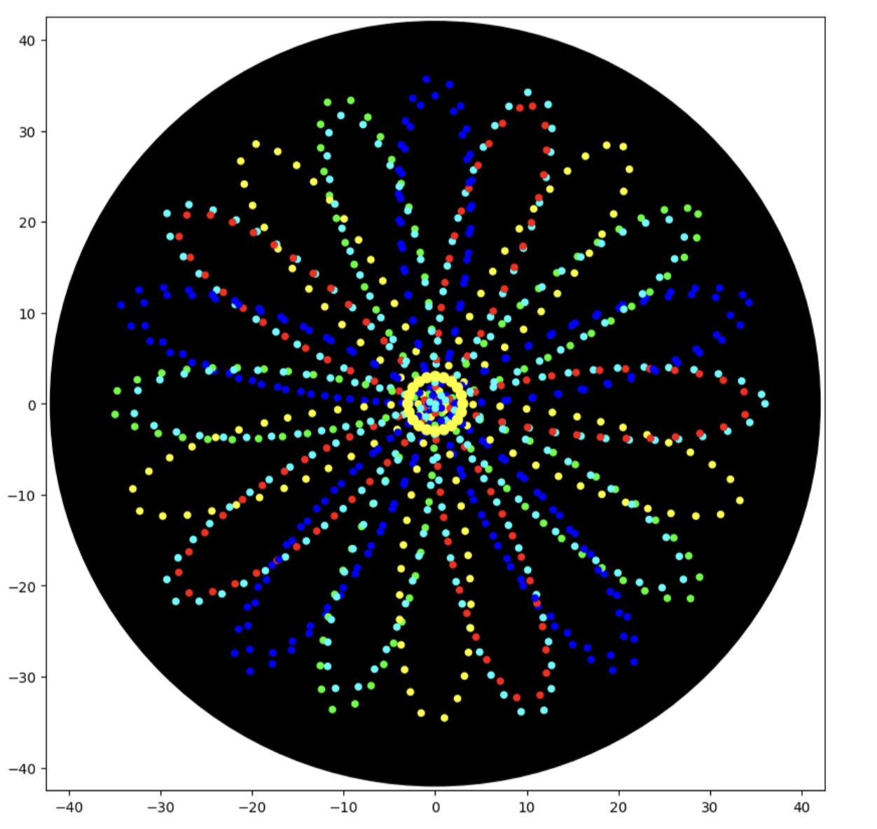
layers = [
    ('cyan',0,1.00,0.2,2.5),
    ('blue',18,1.00,0.2,2.5),
    ('green',36,0.985,0.2,2.5),
    ('yellow',54,0.97,0.2,2.5),
]

Instead of drawing a single curve, the protocol draws multiple layers.

Each layer specifies:

• a color
• a rotation angle
• a scale factor
• droplet size
• spacing between droplets

By rotating and slightly scaling each layer, the curves weave together into a complex multi-color pattern.

for color, rot_deg, scl, dot_ul, step_mm in layers:
    pts = scale_points(base_pts, scl)
    pts = rotate_points(pts, rot_deg)
    dispense_path(color, pts)

ring_pts = []
for i in range(80):
    t = 2 * math.pi * i / 80
    ring_pts.append((ring_r * math.cos(t), ring_r * math.sin(t)))

Finally, a small circular ring of yellow droplets is added at the center of the design.

This creates a visual “sparkle” effect and highlights the symmetry of the pattern.