Week 4 HW: Protein Design Part 1

Protein in 500 g of meat:
100 g → 26 g protein
500 g → 130 g protein

Mass of one amino acid:
1 Dalton = 1.66 × 10⁻²⁴ g
Average amino acid ≈ 100 Da
→ 100 × 1.66 × 10⁻²⁴ = 1.66 × 10⁻²² g

Number of amino acid molecules:
130 g ÷ 1.66 × 10⁻²² g ≈ 7.83 × 10²³ molecules

Convert to moles using Avogadro’s number:
7.83 × 10²³ ÷ 6.022 × 10²³ ≈ 1.30 mol

Final answer:
≈ 7.8 × 10²³ amino acid molecules
≈ 1.3 mol of amino acids

When we eat beef or fish, the body breaks it down into basic building blocks like amino acids, so at that point it is no longer “cow” or “fish” but just raw materials that we use to build our own cells and proteins; the DNA in food is also broken down and cannot function in our bodies, and since our cells only follow human DNA instructions, we are simply using the materials rather than becoming what we eat.

It is not fully understood why there are only 20 natural amino acids. One idea, proposed by Francis Crick, is the frozen accident theory, which suggests that the genetic code is not perfectly optimized but instead came from an early, somewhat arbitrary setup that later became fixed. In that sense, the 20 amino acids we see today may have just been what happened to get locked in at the start of life. At the same time, studies suggest these amino acids cover a good spread of chemical properties—like charge, polarity, hydrophobicity, and size—so they are diverse enough to build a wide range of protein structures.

Yes you can create non-natural amino acids. A well known example is the work by Floyd E. Romesberg, particularly the paper A Genomically Recoded Organism with an Expanded Genetic Alphabet (Nature, 2014), which demonstrated that the genetic alphabet can be expanded by introducing unnatural base pairs. This allows cells to encode and incorporate non-natural amino acids into proteins by creating new codons.

Amino acids likely formed before life through simple chemistry on early Earth rather than through enzymes. A classic example is the experiment by Stanley Miller, who showed in his 1953 Science paper that if you simulate early Earth conditions (basic gases plus an energy source like lightning), amino acids can form spontaneously. This lines up with ideas going back to Charles Darwin, who speculated that life might have first emerged in a warm little pond with the right chemicals and energy. So the building blocks of life can arise from pretty simple ingredients without any biology involved, and interestingly, even now we still haven’t been able to create life itself from scratch.

Because D-amino acids are mirror images of L-amino acids, they naturally form the opposite helix. So while normal L amino acids form right-handed α-helices, D-amino acids form left-handed ones.

Yes, proteins can form additional types of helices beyond the standard α-helix. These include 3₁₀-helices and π-helices, which differ in how tightly they coil and in their hydrogen bonding patterns.

Most molecular helices are right-handed because biological building blocks are chiral with L-amino acids and D-sugars favoring right-handed structures that minimize steric clashes and optimize hydrogen bonding. Exceptions like Z-DNA exist but are less common and form under specific conditions.

This happens because the edges of β-sheets can easily form hydrogen bonds with other strands, and many of the side chains involved are hydrophobic, so they cluster together to avoid water. The main driving force is therefore hydrophobic interactions, along with additional stabilization from hydrogen bonding between sheets.

Amyloid diseases form β-sheets because they are very stable, so misfolded proteins stack into insoluble “cross-β” fibrils that build up over time, as seen in Alzheimer’s Disease, Type 2 Diabetes, and Creutzfeldt–Jakob disease; that same stability also makes these structures useful as materials like nanofibers and scaffolds.

I selected green fluorescent protein (GFP) because it is a well-known protein that clearly links structure to function. GFP naturally fluoresces due to a chromophore formed within its folded structure, which makes it widely used to track gene expression and protein location in cells. I also chose it because I’ve enjoyed working with fluorescent systems in biology so far, like in the Opentrons lab, so it feels familiar and intuitive while still being a powerful example of how protein structure leads to function.

From CBI I obtained the amino acid sequence - Aequorea victoria green-fluorescent protein:
https://www.ncbi.nlm.nih.gov/nuccore/L29345.1

MSKGEELFTGVVPILVELDGDVNGQKFSVSGEGEGDATYGKLT
KFICTTGKLPVPWPTLVTTFSYGVQCFSRYPDHMKQHDFFKSAMPEGYVQERTIFFKD
DGNYKTRAEVKFEGDTLVNRIELKGIDFKEDGNILGHKMEYNYNSHNVYIMADKPKNG
IKVNFKIRHNIKDGSVQLADHYQQNTPIGDGPVLLPDNHYLSTQSALSKDPNEKRDHM
ILLEFVTAAGITHGMDELYK

sp|Q15465|SHH_HUMAN Sonic hedgehog protein Results
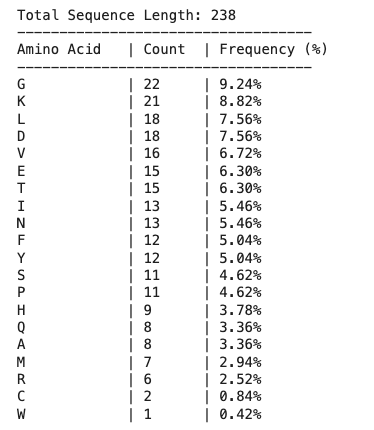
Length: 238 amino acids
Most frequent: G (22 times, 9.2%)

How many protein sequence homologs are there for your protein?

Uniprot id: P42212 - 205 hits found

Does your protein belong to any protein family?

GFP belongs to the green fluorescent protein (GFP) family. This family includes a range of fluorescent proteins found in organisms like jellyfish and corals, all of which share a similar β-barrel structure and fluorescent chromophore but can emit different colors (e.g. green, blue, cyan, yellow, red).

https://www.rcsb.org/3d-view/1EMA - 1EMA structure for GFP

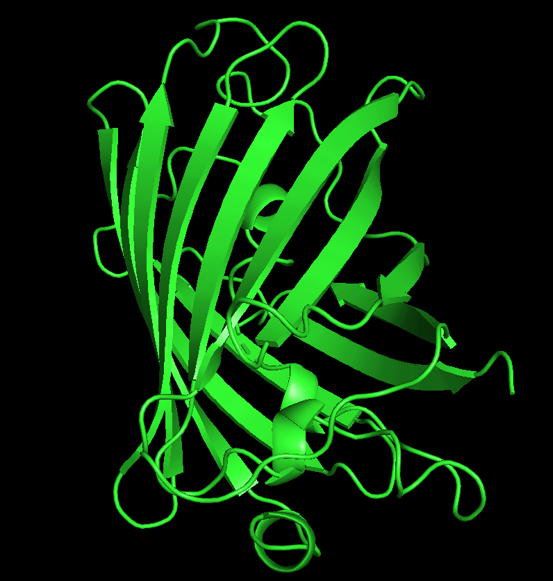
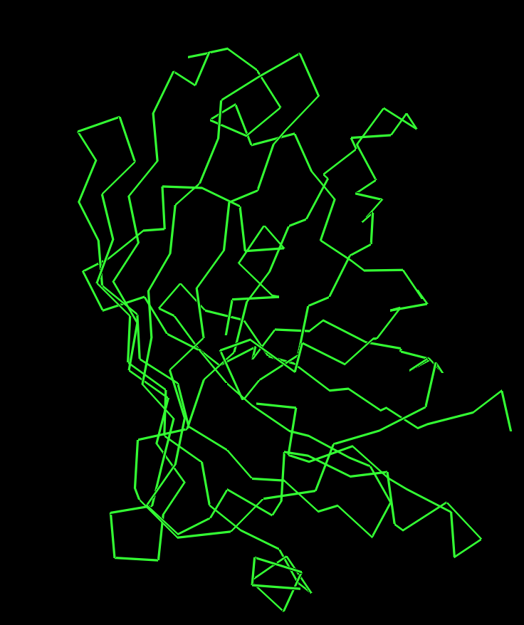
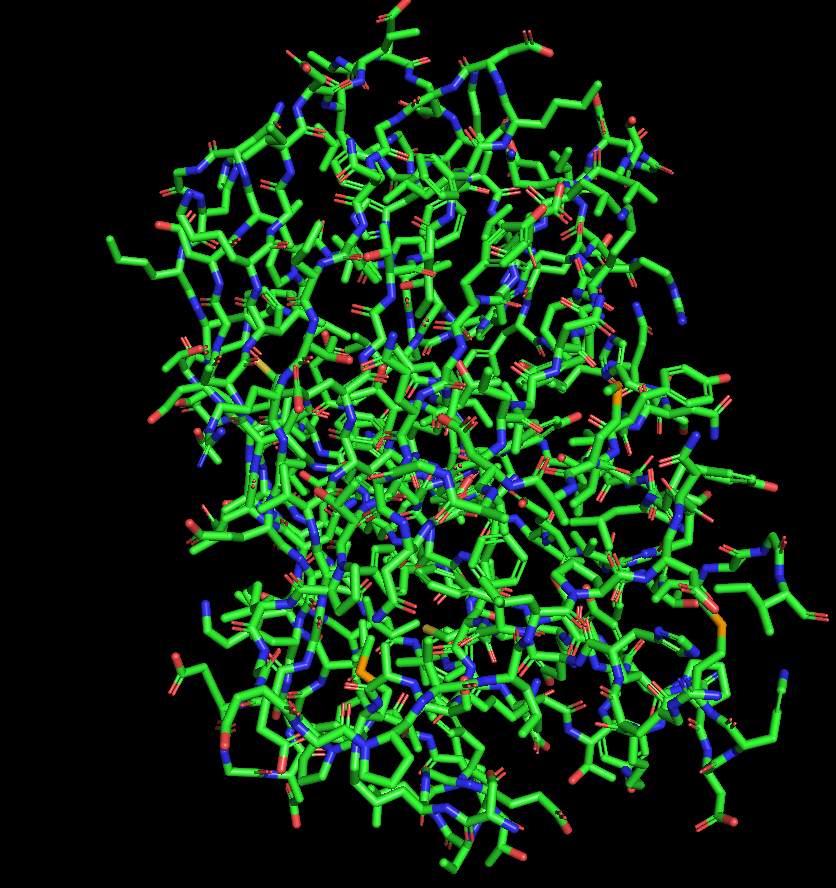
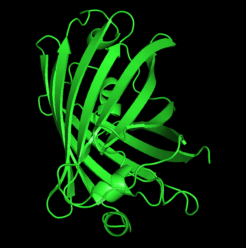
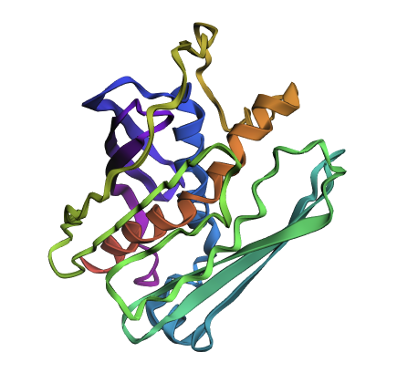
The GFP structure (PDB ID: 1EMA) was solved in 1996, deposited on August 1 and released on November 8 by Ormo and Remington. It was determined using X-ray diffraction with a resolution of 1.90 Å, indicating a high-quality structure with well-resolved atomic positions. In addition to the protein, the structure includes water molecules and the chromophore (listed as a non-standard residue). Structurally, GFP belongs to the all-β β-barrel fold, commonly referred to as the GFP-like fold in classification systems such as SCOP.

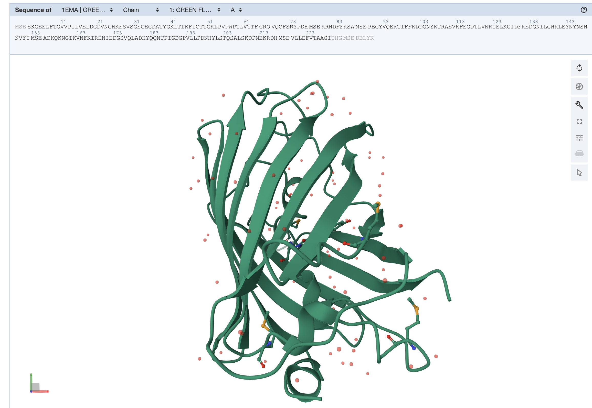
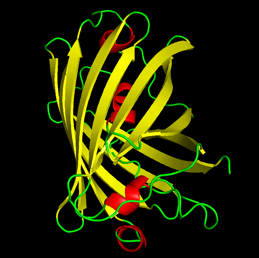
dss
color red, ss h
color yellow, ss s
color green, ss l

From the structure, we can infer that hydrophobic residues are predominantly located in the interior of the protein, forming a stable core, while hydrophilic residues are mainly exposed on the surface where they can interact with the surrounding aqueous environment. This distribution is consistent with typical protein folding and helps stabilize the β-barrel structure of GFP.

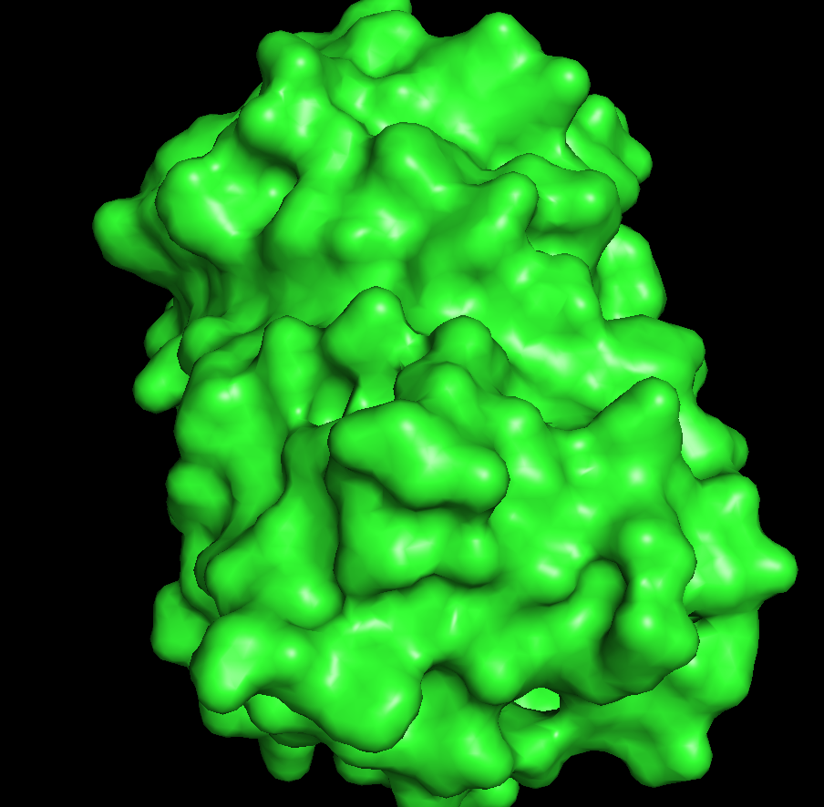
The protein appears mostly smooth and compact with no large exposed binding pockets on the exterior. There are only small surface indentations, but no obvious deep cavities. This suggests that GFP does not have a typical surface binding site; instead, its main “hole” is an internal cavity within the β-barrel, which is not visible from the outside surface.

At a high level, we are using a pretrained machine learning model to learn patterns from large numbers of protein sequences and then apply that knowledge to analyze a specific protein. In the deep mutational scan, we systematically mutate each position in the protein and use the model to estimate how likely or tolerated each mutation is, which helps identify important versus flexible regions of the protein. In latent space analysis, we convert entire protein sequences into vector embeddings and visualize them in a reduced-dimensional space, where proteins with similar structure or function cluster together. Together, these approaches let us explore both how individual mutations affect a protein and how whole proteins relate to each other, without directly simulating their physical behavior.

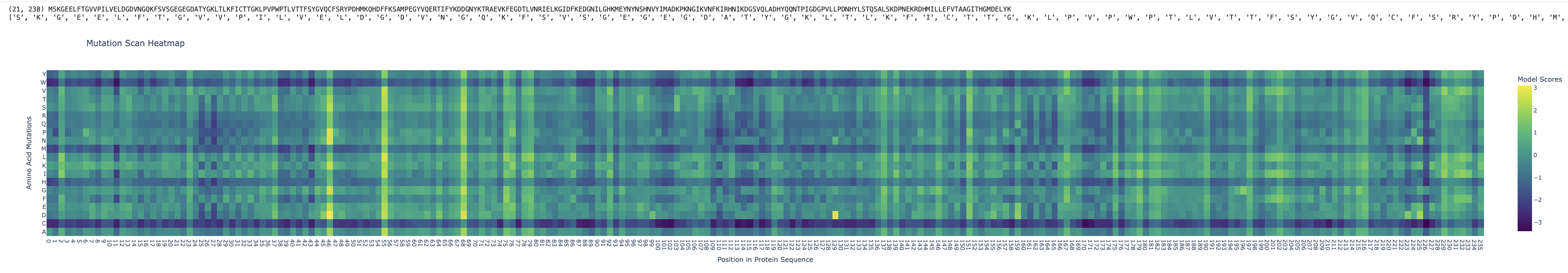
The mutation scan heatmap shows how each possible amino acid substitution affects every position in the protein. The x-axis represents the position along the protein sequence (from residue 1 to ~238 for GFP), and the y-axis represents the 20 possible amino acids that could be substituted at each position. Each cell in the heatmap corresponds to a specific mutation (e.g. position i mutated to amino acid j), and the color indicates the model’s score or likelihood for that mutation: brighter colors (yellow/green) indicate mutations that are more likely or tolerated, while darker colors (blue/purple) indicate mutations that are unlikely and likely destabilizing.

By looking vertically at a single column (one position), we can see how sensitive that position is to mutation, columns that are mostly dark suggest highly conserved, functionally or structurally critical residues, whereas columns with many lighter colors indicate positions that are more flexible and tolerant to change. Patterns across the heatmap therefore reveal which regions of the protein are constrained (e.g. core or active regions) versus more variable (e.g. surface or loop regions), giving insight into the protein’s stability and function.

For example, at a position in the core of the protein (e.g. around residue ~65, near the chromophore region in GFP), most substitutions are dark (low likelihood), but mutations to similar amino acids (e.g. hydrophobic → hydrophobic) may be slightly less penalized. This suggests that the residue is highly conserved and structurally important, and changing it disrupts the local environment required for stability or function. In contrast, substituting with a chemically similar residue is less disruptive, which is why those mutations appear slightly more tolerated.

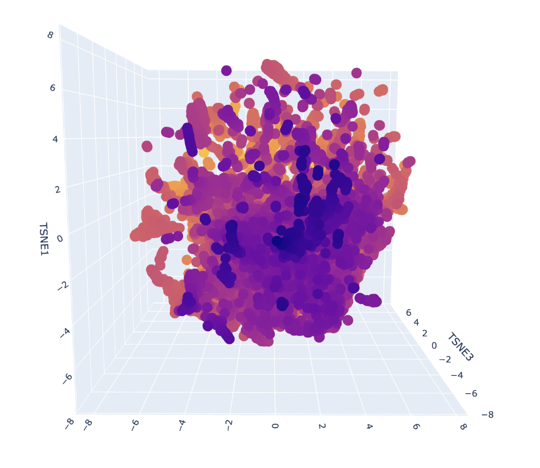
Each point represents a protein, and proximity reflects similarity in learned sequence features. After placing GFP into this space, its nearest neighbor was another GFP sequence, confirming the model correctly captures sequence similarity. However, other nearby proteins were functionally different and relatively distant, suggesting that GFP is somewhat isolated in this dataset due to a lack of closely related sequences. This indicates that while the latent space captures meaningful relationships, the dataset composition strongly influences the observed neighborhoods.

Protein folding is important because a protein’s function is determined by its three-dimensional structure rather than just its amino acid sequence. The way a protein folds defines its active sites, binding interactions, and overall stability, which in turn controls how it behaves in a biological system. Misfolding can lead to loss of function or disease, while correct folding enables proteins to carry out roles such as catalysis, signaling, and structural support. Being able to understand and predict how a sequence folds therefore allows us to infer function, study the effects of mutations, and design new proteins or therapeutics without relying solely on experimental methods.

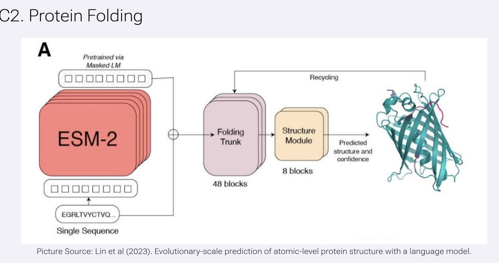
In this task, we used ESMFold to predict protein structure directly from sequence. The model is first pretrained as a protein language model (ESM-2), learning patterns from large datasets of sequences, and then passes this information into a folding module that outputs predicted 3D coordinates. In the diagram, the sequence is encoded into embeddings, processed through a series of network blocks, and iteratively refined to produce a final structure along with a confidence estimate. We then compare the predicted structure to known experimental structures and test how mutations affect folding, allowing us to explore how robust the protein’s structure is to changes in its sequence.

Inverse protein folding is the process of starting with a desired 3D protein structure (its backbone shape) and designing an amino acid sequence that will fold into that structure. Instead of predicting structure from a sequence, you reverse the problem: given a fixed geometry, a model like ProteinMPNN selects residues that fit spatially, stabilize interactions, and satisfy physical constraints. Because many different sequences can produce the same structure, the goal is to find one (or several) that make the structure energetically stable. The designed sequence is then typically validated by folding it again with a model like ESMFold and checking whether it reproduces the original structure.