Week 10 HW: Imaging & Measurement Technology

For my final project, I would measure whether GFP was successfully conjugated to magnetic beads and whether those GFP-coated magnetic beads can activate anti-GFP synNotch/SNIPR-style receptors in cells. The main thing I care about is whether magnetic presentation of the ligand changes receptor activation compared to normal soluble GFP.

First, I would measure GFP attachment to the magnetic beads. I could do this by measuring the fluorescence of the supernatant before and after conjugation. If GFP successfully binds to the beads, the remaining supernatant should become less fluorescent because less free GFP is left in solution. I could also image the beads under a fluorescence microscope to see whether the magnetic particles show green fluorescence, although this is more qualitative. A more quantitative method would be using a plate reader to compare GFP fluorescence in the starting solution, wash fractions, and final bead fraction.

Second, I would measure whether the cells are actually receiving and expressing the synNotch receptor and reporter plasmids. This could be checked using fluorescence microscopy or flow cytometry if the system includes a reporter such as mNeonGreen, mKO2, or eBFP2. Flow cytometry would be especially useful because it would let me quantify what percentage of cells are fluorescent and how strong the signal is per cell.

Third, I would measure synNotch activation itself. The output would be reporter expression downstream of the UAS promoter, such as mNeonGreen or another fluorescent protein. I would compare cells exposed to soluble GFP, GFP-conjugated magnetic beads without a magnet, and GFP-conjugated magnetic beads with magnetic guidance. If the magnetic system works, I would expect stronger or more spatially localized reporter expression in the magnetic bead condition.

The main technologies I would use are fluorescence microscopy, plate reader fluorescence measurements, magnetic separation, and potentially flow cytometry. Fluorescence microscopy would show where the GFP-beads are located and whether reporter activation is spatially patterned. A plate reader would give a bulk quantitative measurement of GFP conjugation and reporter output. Flow cytometry would give a more precise single-cell measurement of activation across the cell population. Together, these measurements would let me test both parts of the project: whether the magnetic GFP ligand was made successfully, and whether it can control synthetic receptor activation in cells.

To calculate the theoretical molecular weight of eGFP, we used the full amino acid sequence provided, including the eGFP core protein, the LE linker, and the 6x-His purification tag. The sequence was entered into the ExPASy Compute pI/Mw tool, which calculates the predicted molecular weight based on the amino acid composition of the protein.

The calculated theoretical molecular weight was 27,988.97 Da. This value represents the expected mass of the intact eGFP protein before experimental measurement by mass spectrometry.

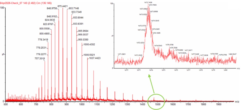
To experimentally determine the molecular weight of eGFP from the mass spectrum, we used the adjacent charge state method. In electrospray ionization mass spectrometry (ESI-MS), proteins acquire multiple positive charges, producing a series of peaks corresponding to different charge states. By selecting two adjacent peaks, we can calculate the charge state and then determine the molecular weight.

We selected two adjacent peaks from the spectrum:

• Peak 1: 875.4421 m/z
• Peak 2: 903.7148 m/z

We used the charge state equation:

Substituting the values:

Rounding to the nearest integer gives a charge state of 32+ for the 875.4 peak and 31+ for the 903.7 peak.

Using the 32+ charge state:

Therefore, the experimentally determined molecular weight of eGFP was 27,981.90 Da.

To compare the experimental value to the theoretical value, we calculated the error in parts per million (ppm):

Substituting the values:

This shows that the experimentally measured molecular weight was very close to the predicted theoretical mass.

No, the individual isotopic charge state peaks cannot be clearly resolved in the zoomed-in spectrum. This is because the protein is detected in a highly charged denatured state around 32+, meaning the isotopic peak spacing becomes very small:

At this spacing, the peaks are too close together for a mass spectrometer with a resolution of 30,000 to distinguish individually. Instead of separate isotopic peaks, the signal appears as a broad unresolved isotopic envelope.

We will analyze eGFP in its native, folded state and compare it to its denatured, unfolded state on a quadrupole time-of-flight MS. We will be doing MS-only analysis (no liquid chromatography, also known as “direct infusion” experiments) on the Waters Xevo G3-QToF MS.

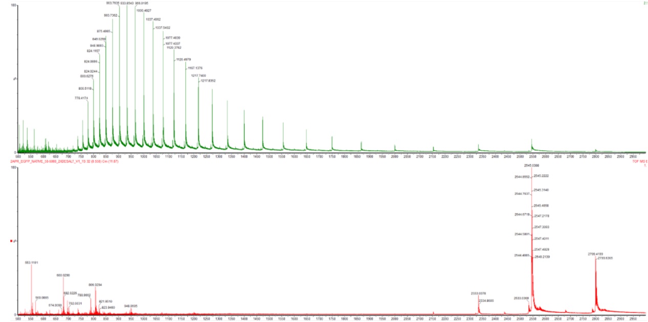
In the denatured state, the protein becomes unfolded, usually due to acidic solvents, organic solvents, or heat. This unfolding exposes many basic amino acid residues such as lysine, arginine, and histidine that were previously buried inside the protein structure. Because more protonation sites become accessible, the protein picks up many protons during electrospray ionization, leading to high charge states. As a result, the denatured protein appears at lower m/z values in the mass spectrum, typically in the ~500–1500 m/z range.

In the native state, the protein remains folded in its normal 3D conformation. For eGFP, this corresponds to its compact beta-barrel structure. Since many basic residues remain buried within the folded protein, fewer sites are available for protonation. Consequently, the protein acquires fewer charges and appears at higher m/z values in the mass spectrum, typically in the ~2000–4000 m/z range.

By comparing the spectra, we observe that the denatured spectrum contains a broad distribution of many highly charged peaks at low m/z, whereas the native spectrum contains fewer charge states shifted toward much higher m/z values. This reflects the difference between an unfolded and compact folded protein structure.

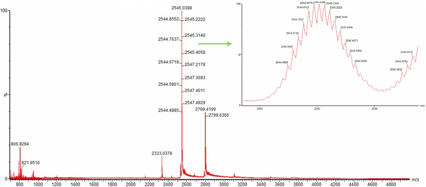
Yes. The charge state of the peak at ~2800 m/z is 10+.

To determine this, we examine the zoomed-in isotopic distribution shown in Figure 3. The individual isotopic peaks are clearly resolved, and the spacing between adjacent isotopes is approximately 0.1 m/z.

In mass spectrometry, isotopic peak spacing is equal to 1/z, where z is the charge state.

Since the observed spacing is ~0.1 m/z:

Therefore the peak corresponds to a 10+ charge state.

We will digest the eGFP protein standard into peptides using trypsin (an enzyme that selectively cleaves the peptide bond after Lysine (K) and Arginine (R) residues. The resulting peptides will be analyzed on the Waters BioAccord LC-MS to measure their molecular weights and fragmented to confirm the amino acid sequence within each peptide – generating a “peptide map”. This process is used to confirm the primary structure of the protein.

There are a variety of tools available online to calculate protein molecular weight and predict a list of peptides generated from a tryptic digest. We will be using tools within the online resource Expasy (the bioinformatics resource portal of the Swiss Institute of Bioinformatics (SIB)) to predict a list of tryptic peptides from eGFP.

To determine how many trypsin cleavage sites exist in eGFP, we analyzed the amino acid sequence and counted the number of Lysine (K) and Arginine (R) residues, since trypsin specifically cleaves after K and R residues.

From the sequence analysis, eGFP contains:

• 20 Lysines (K)
• 6 Arginines (R)

These residues define the locations where trypsin can digest the protein into smaller peptide fragments.

To predict the number of peptides produced after digestion, we used the PeptideMass tool from ExPASy. The full eGFP amino acid sequence was entered into the program and digested in silico using trypsin with zero missed cleavages.

The prediction generated:

This represents the theoretical number of peptide fragments expected after complete tryptic digestion.

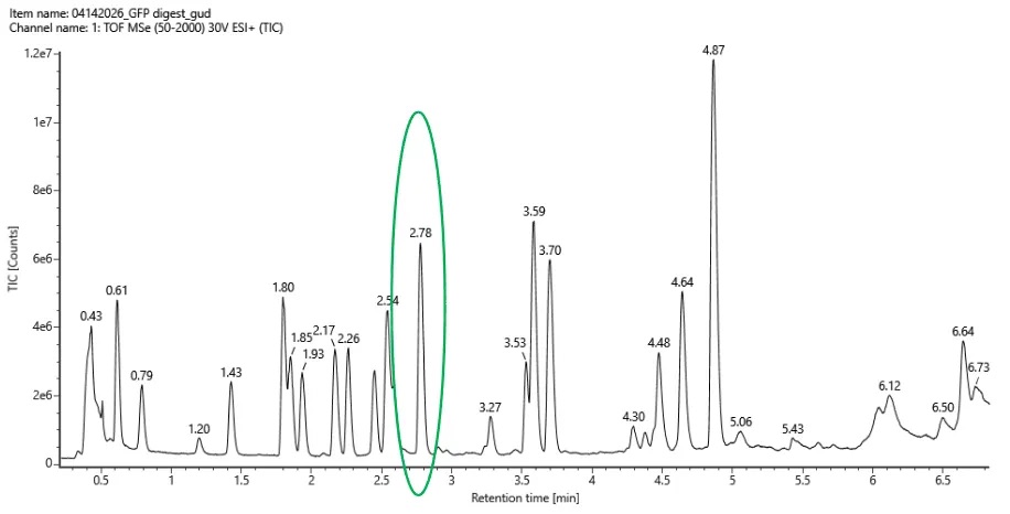
We examined the Total Ion Chromatogram (TIC) shown in Figure 5a and counted peaks with greater than 10% relative abundance between 0.5 and 6 minutes retention time.

Approximately:

Each peak likely corresponds to one or more peptides eluting from the LC column during the separation.

No. The number of observed chromatographic peaks does not exactly match the predicted number of peptides.

• Predicted peptides: 27
• Observed peaks: 18

This difference is expected in LC-MS peptide mapping because some peptides may be too small to retain on the chromatography column, some may co-elute at the same retention time, and others may ionize poorly or fall below the detection threshold.

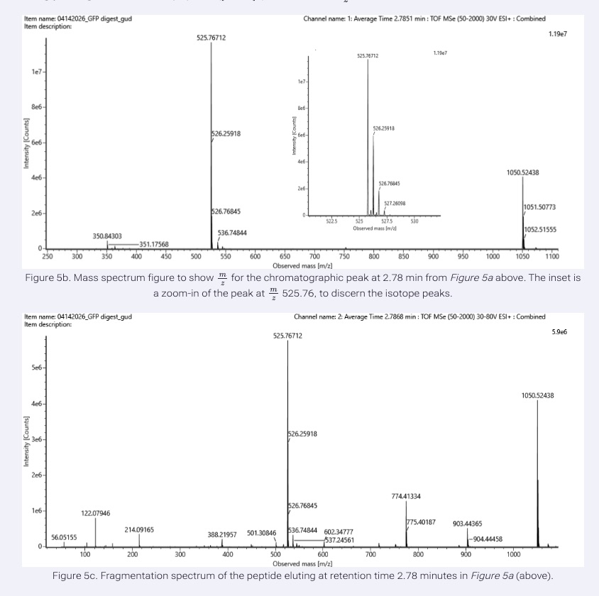
From Figure 5b, the most abundant peptide peak was observed at:

• m/z = 525.76712

To determine the charge state, we examined the isotope spacing in the zoomed-in spectrum. The isotopic peaks were separated by approximately:

Since isotopic spacing equals 1/z, we calculate:

Therefore, the peptide has a:

• 2+ charge state

To calculate the singly charged mass (MH+):

Substituting the values:

Thus, the singly charged peptide mass is:

• 1050.53 Da

The experimentally measured peptide mass was compared with the predicted peptide list generated by PeptideMass.

The peptide was identified as:

The theoretical singly charged mass for this peptide is:

The experimental mass accuracy was calculated in parts per million (ppm):

The calculated error was:

This very small error indicates high confidence in the peptide identification.

Using the peptide mapping results shown in Figure 6, the LC-MS analysis confirmed:

This means that peptides corresponding to 88% of the amino acid sequence of eGFP were experimentally detected and identified.

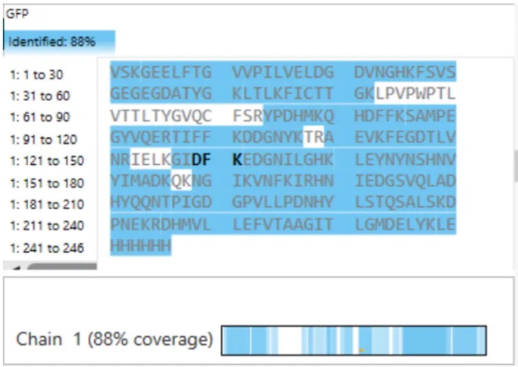
The fragmentation spectrum in Figure 5c corresponds to the peptide:

This was determined by matching the observed fragment ions to the expected b-ion and y-ion fragmentation pattern generated from this peptide sequence.

Yes. The peptide map data is highly consistent with the expected eGFP protein standard.

The experiment achieved:

• High sequence coverage (88%)
• High mass accuracy (5.7 ppm)
• Matching fragmentation spectra for identified peptides

Together, these results strongly confirm that the analyzed protein is eGFP and demonstrate successful peptide mapping using LC-MS/MS.

We will determine Keyhole Limpet Hemocyanin (KLH)’s oligomeric states using charge detection mass spectrometry (CDMS). CDMS single-particle measurements of KLH allow us to make direct mass measurements to determine what oligomeric states (that is, how many protein subunits combine) are present in solution. Using the known masses of the polypeptide subunits (Table 1) for KLH, identify where the following oligomeric species are on the spectrum shown below from the CDMS (Figure 7):

• 7FU Decamer
• 8FU Didecamer
• 8FU 3-Decamer
• 8FU 4-Decamer

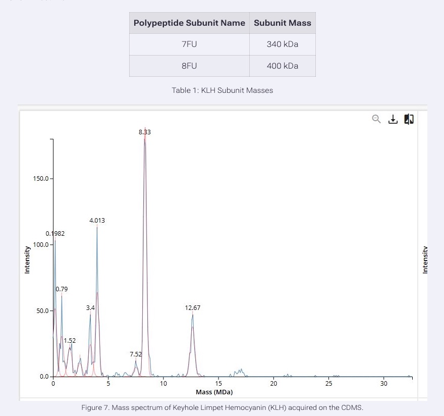
Based on the CDMS mass spectrum and the known KLH subunit masses, the oligomeric states can be assigned by multiplying the subunit mass by the number of subunits present.

The 7FU decamer contains 10 copies of the 7FU subunit. Since each 7FU subunit is 340 kDa, the expected mass is about 3.4 MDa, which matches the peak observed at 3.4 MDa.

The 8FU didecamer contains 20 copies of the 8FU subunit. Since each 8FU subunit is 400 kDa, the expected mass is about 8.0 MDa, which corresponds closely to the large peak observed at 8.33 MDa.

The 8FU 3-decamer contains 30 copies of the 8FU subunit, giving an expected mass of about 12.0 MDa. This matches the peak observed at 12.67 MDa.

The 8FU 4-decamer contains 40 copies of the 8FU subunit giving an expected mass of about 16.0 MDa. This would correspond to the lower-abundance peaks furthest to the right, around 16 to 17 MDa.

Please fill out this table with the data you acquired from the lab work done at the Waters Immerse Lab in Cambridge, or else the data screenshots in this document if you were unable to have lab work done at Waters.