Week 4 HW: Protein Design Part I

This page tackles all homeworks of week 4.

Part A. Conceptual Questions

Part B: Protein Analysis and Visualization

Questions	Answers
1. Briefly describe the protein you selected and why you selected it.	I selected the protein Ubiquitin for this assignment. Ubiquitin is a small regulatory protein found in eukaryotic cells that plays an important role in protein degradation, signalling, and cellular regulation. It has a well-characterised three-dimensional structure, and many experimentally determined structures are available in the Protein Data Bank (PDB). I initially considered using GB1, but found that its initiator methionine is retained in the mature protein. Since my broader project involves studying retro (reverse) protein sequences, I wanted a protein in which the initial methionine is naturally removed during post-translational processing. In many proteins, the initiator methionine is cleaved by methionine aminopeptidase when the second amino acid has a small side chain. Ubiquitin is therefore a suitable choice because its mature form does not retain the starting methionine, allowing cleaner comparison between the natural sequence and a retro/reverse sequence without introducing an artificial terminal methionine residue. Additionally, ubiquitin is small, structurally stable, and extensively studied, making it convenient for computational and structural analysis.
2. Identify the amino acid sequence of your protein. How long is it? What is the most frequent amino acid? You can use this Colab notebook to count the frequency of amino acids. How many protein sequence homologs are there for your protein? Hint: Use Uniprot’s BLAST tool to search for homologs. Does your protein belong to any protein family?	The protein I selected is Ubiquitin from humans, a highly conserved regulatory protein involved in protein degradation and cellular signalling. Ubiquitin. The mature amino acid sequence of UBIQUITIN is QIFVKTLTGKTITLEVEPSDTIENVKAKIQDKEGIPPDQQRLIFAGKQLEDGRTLSDYNIQKESTLHLVLRLRGG; it contains 75 amino acids with the most frequent AA being Leucine (L appears 9 times, frequency 11.84%). Lysine (K) is also highly abundant and biologically important because ubiquitin forms polyubiquitin chains through lysine residues. Ubiquitin has thousands of homologs across eukaryotes because it is one of the most evolutionarily conserved proteins known. Human and yeast ubiquitin, for example, share about 96% sequence identity, differing in only 3 out of 76 amino acids; (these were validated using UniProt BLAST). Ubiquitin belongs to the Ubiquitin protein family (Pfam accession: PF00240), a family of small regulatory proteins involved in ubiquitination and intracellular protein turnover. Members of this family are small proteins or protein domains that adopt the characteristic ubiquitin fold. Proteins in this family are involved in post-translational modification pathways and intracellular protein turnover.
3. Identify the structure page of your protein in RCSB. When was the structure solved? Is it a good quality structure? Good quality structure is the one with good resolution. Smaller the better (Resolution: 2.70 Å). Are there any other molecules in the solved structure apart from protein? Does your protein belong to any structure classification family?	The structure page of my protein is available in the Protein Data Bank (RCSB PDB) under the entry 1UBQ titled “Structure of ubiquitin refined at 1.8 Å resolution.” The structure was solved in 1987 using X-ray diffraction, with the reported resolution indicating a very high-quality protein structure. In structural biology, lower resolution values correspond to more accurate atomic positions, and structures below about 2.0 Å are generally considered excellent quality. Apart from the protein itself, the solved structure also contains water molecules that were resolved in the crystal structure. No additional ligands or cofactors are present in the basic ubiquitin structure. Ubiquitin belongs to the ubiquitin fold structural family, a highly conserved protein fold characterized by a compact globular structure containing β-sheets and an α-helix. It is also classified within the Ubiquitin-like superfamily in structural classification databases such as SCOP and CATH. Members of this structural family are involved in protein regulation, signalling, and intracellular protein turnover.
4. Open the structure of your protein in any 3D molecule visualization software: PyMol Tutorial Here (hint: ChatGPT is good at PyMol commands). Visualize the protein as “cartoon”, “ribbon” and “ball and stick”. Colour the protein by secondary structure. Does it have more helices or sheets? Colour the protein by residue type. What can you tell about the distribution of hydrophobic vs hydrophilic residues? Visualize the surface of the protein. Does it have any “holes” (aka binding pockets)?	I used RCSB's 3D Viewer to visualize ubiquitin in cartoon, ribbon, molecular surface, ball-and-stick, and spacefill representations.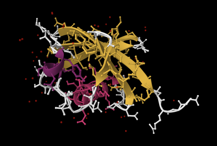 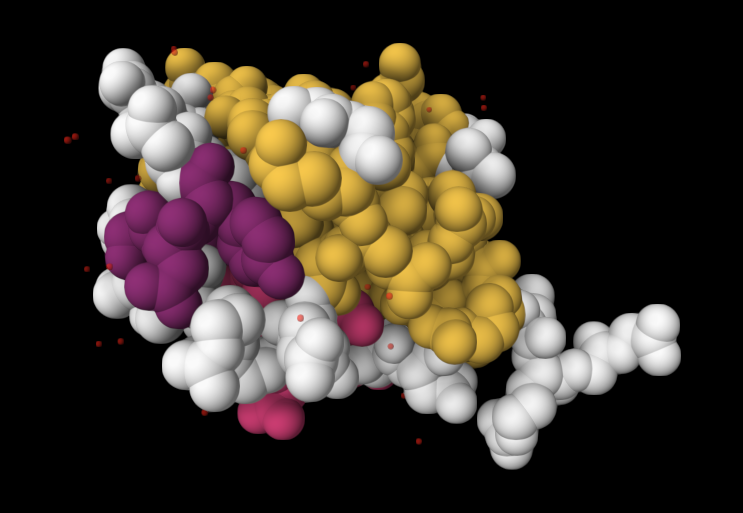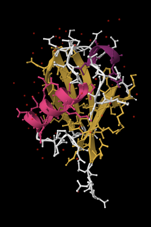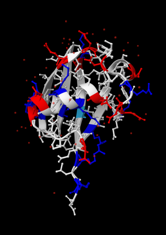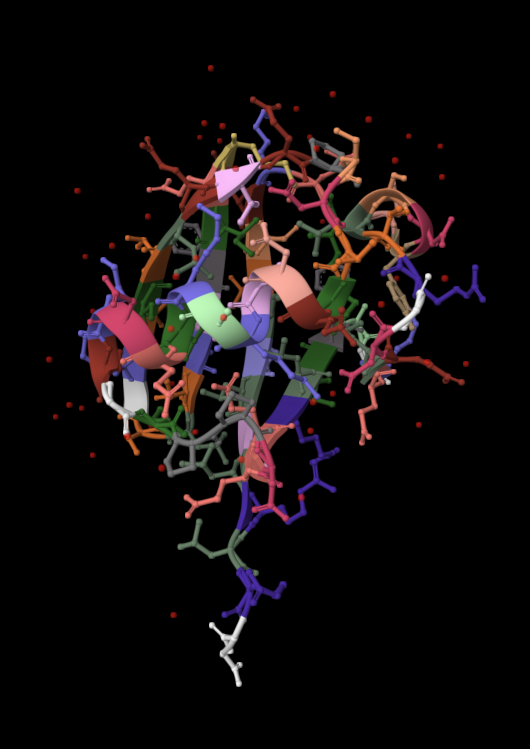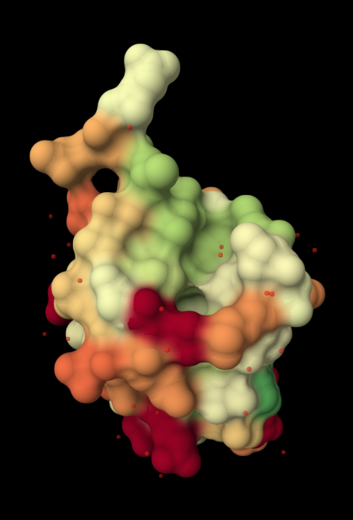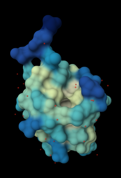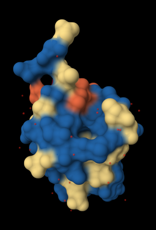Ubiquitin contains more β-sheets than α-helices (consistent with the characteristic ubiquitin β-grasp fold). Hydrophobic residues are mainly buried in the interior core, while charged and hydrophilic residues are exposed on the surface. It has one hole (binding pocket). Surface visualization shows a compact globular structure with shallow interaction grooves rather than deep catalytic binding pockets.

Part C. Using ML-Based Protein Design Tools

Questions	Answers
C1.1. Deep Mutational Scans. Use ESM2 to generate an unsupervised deep mutational scan of your protein based on language model likelihoods. Can you explain any particular pattern? (choose a residue and a mutation that stands out)	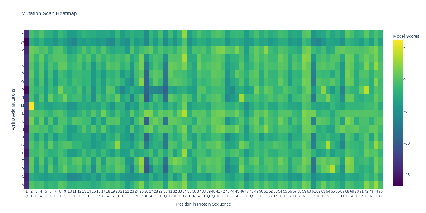The first Amino acid mutation is highly unfavourable to anything. However, peculiarly, the second AA mutation to Methionine (M) is extremely favourable. Does that mean that after the second place mutation to M, the first place AA is removed through post-translational modifications; otherwise in this case there will be an AA before the methionine (M) which generally does not happen as M is the start codon. For the retro protein sequence, the first place's mutation is similarly highly unfavourable but a specific position 40 seems to have many favourable mutations...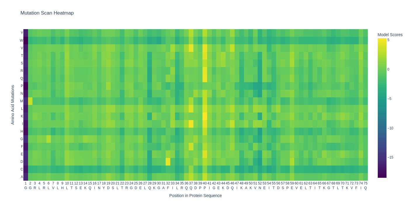
C1.2. Latent Space Analysis: Use the provided sequence dataset to embed proteins in reduced dimensionality. Analyze the different formed neighborhoods: do they approximate similar proteins? Place your protein in the resulting map and explain its position and similarity to its neighbours.	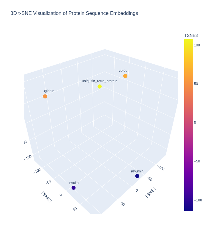Protein sequences were first converted into 320-dimensional latent embeddings using the ESM2 protein language model. These embeddings are numerical representations learned from large-scale evolutionary protein sequence data and encode biochemical, structural, and evolutionary features of proteins. Similar proteins tend to occupy nearby regions in this high-dimensional embedding space. To visualize these embeddings, t-distributed Stochastic Neighbor Embedding (t-SNE) was used to reduce the 320-dimensional vectors into three dimensions. Since only five protein sequences were analyzed, the perplexity parameter was reduced from the default value of 30 to 3 (because t-SNE requires the perplexity value to be smaller than the number of samples). Perplexity approximately controls the effective number of neighboring points considered during dimensionality reduction. Lower perplexity values emphasize local neighborhood relationships between nearby proteins. The three plotted axes (TSNE1, TSNE2, and TSNE3) do not correspond to specific physical or biochemical quantities such as molecular weight, hydrophobicity, or sequence length. Instead, they are abstract latent coordinates generated by t-SNE to preserve local similarity relationships between the original high-dimensional embeddings. Proteins that appear closer together in the plot are interpreted as having more similar learned sequence representations, while proteins farther apart are considered more dissimilar in the latent embedding space. In the resulting embedding map, Ubiquitin and the retro-Ubiquitin sequence occupied different positions despite containing the same amino acid composition in reversed order, suggesting that sequence order strongly influences the learned representation of the protein language model and that the retro sequence is interpreted as biologically distinct from native ubiquitin. Other proteins, such as haemoglobin, insulin, and albumin fragments, also occupied separate regions, reflecting their differing sequence patterns and biological functions. However, t-SNE visualizations should be interpreted qualitatively rather than quantitatively. The distances and cluster sizes in t-SNE plots can vary depending on initialization and parameter choices such as perplexity, and therefore do not represent exact evolutionary or structural distances between proteins.
C2. Protein Folding: Fold your protein with ESMFold. Do the predicted coordinates match your original structure? Try changing the sequence, first try some mutations, then large segments. Is your protein structure resilient to mutations?	ESMFold was used to predict the structure of both native ubiquitin and a retro-ubiquitin sequence generated by reversing the amino acid order. The model directly predicted atomic coordinates from sequence without requiring multiple sequence alignments. The native ubiquitin prediction showed high confidence, with most residues having pLDDT values above 85–90. The PAE heatmap also showed low predicted aligned error across most residue pairs, indicating that the model was confident about the global fold and residue positioning. The predicted structure retained the compact ubiquitin-like fold with well-defined β-sheets and α-helices. pLDDT is a per-residue confidence score ranging from 0–100, where higher values indicate more reliable structural predictions. 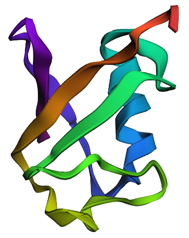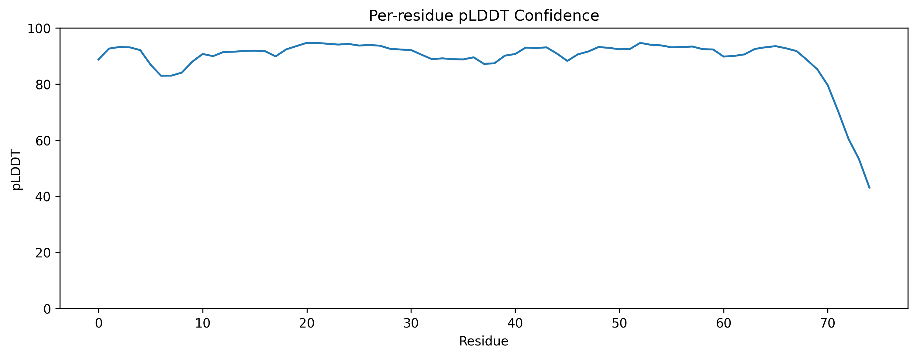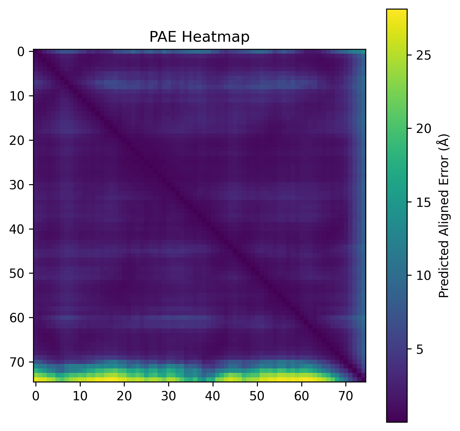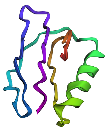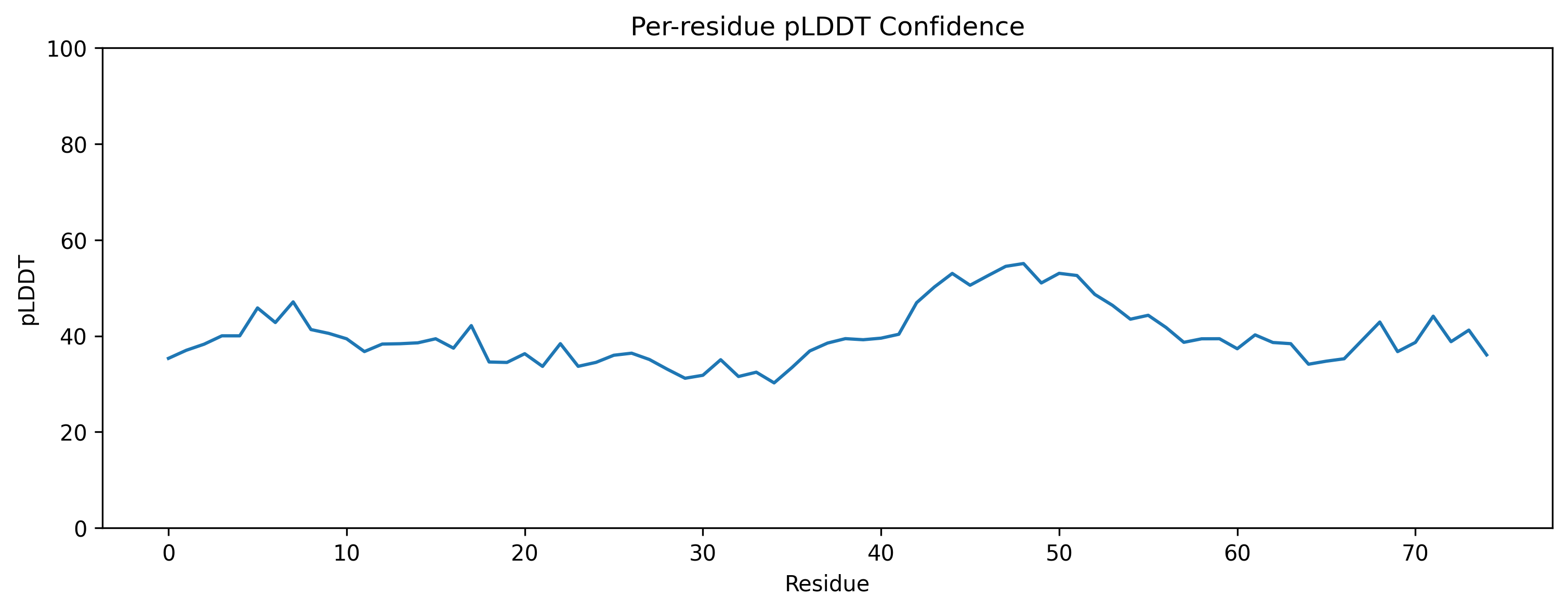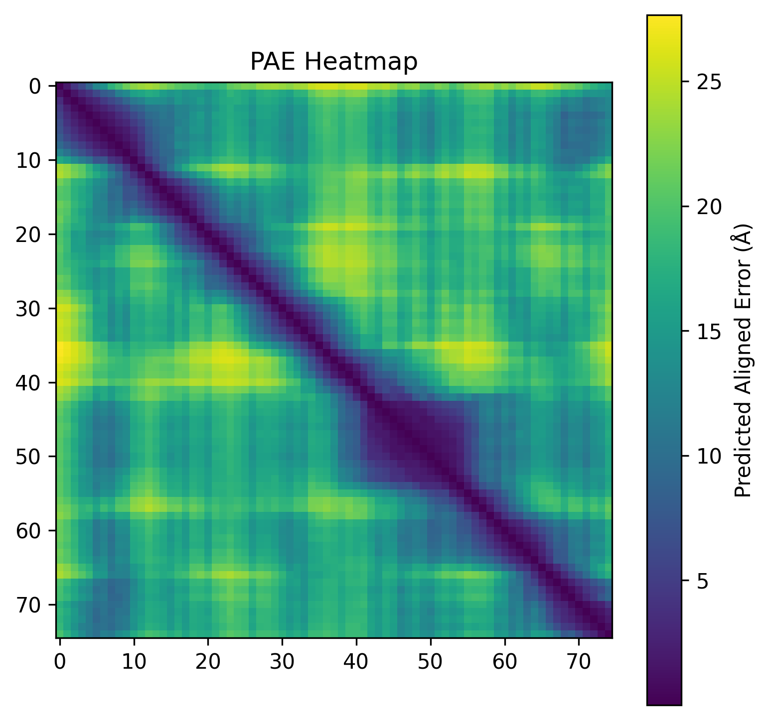In contrast, the retro-ubiquitin model showed much lower pLDDT values (~30–55 across most residues), suggesting low confidence and reduced structural stability. The PAE heatmap also displayed much larger predicted errors across residue pairs, indicating uncertainty in the relative arrangement of structural regions. Even though retro-ubiquitin contains the same residues as native ubiquitin, reversing the sequence disrupts the learned structural and evolutionary patterns required for forming the exact original folds.
C3. Protein Generation: Inverse-Folding a protein: Let’s now use the backbone of your chosen PDB to propose sequence candidates via ProteinMPNN. Analyze the predicted sequence probabilities and compare the predicted sequence vs the original one. Input this sequence into ESMFold and compare the predicted structure to your original.	ProteinMPNN was used to perform inverse folding on the Ubiquitin backbone structure. Instead of predicting structure from sequence, ProteinMPNN predicts amino acid sequences that are compatible with a given protein backbone geometry. The generated heatmap represents the probability of each amino acid occurring at every residue position based on the backbone structure. Bright regions indicate amino acids strongly preferred by the model at specific positions, while diffuse regions represent positions that tolerate greater sequence variability.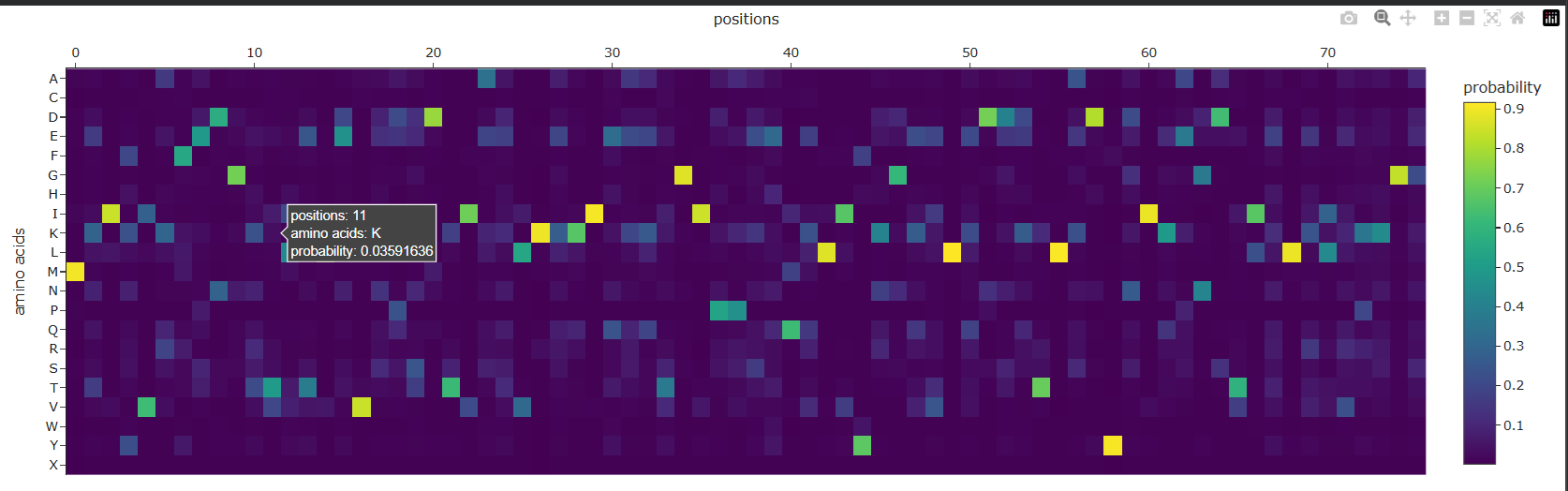 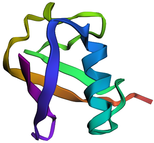The designed sequence differed substantially from native Ubiquitin while still remaining compatible with the same backbone fold. The sequence recovery value was ~54%, indicating that roughly half of the residues were conserved relative to the original sequence. Structurally important positions showed stronger conservation, whereas surface or flexible positions tolerated more substitutions. Interestingly, the generated sequence achieved a lower ProteinMPNN score than the native sequence, suggesting that the designed sequence may fit the backbone geometry more favorably (according to the model!). This demonstrates that many different amino acid sequences can potentially encode similar protein folds, highlighting the robustness and degeneracy of protein structural organization. Original: -Q-F-K-LT-K------E-S---ENV-A--QD-E----DQ----FA-KQ-E-GR--S----QKES--H-V-RLR-- Generated: -T-Y-E-ED-T------S-D---AEL-K--EE-T----EE----YK-EE-K-DK--A----KEGD--K-E-VPK--

Part D. Group Brainstorm on Bacteriophage Engineering

Since I am solo, I am proposing Recursive Protein Optimization using beam-search over Mutation Space: considering ESM2 likelihoods, conditional mutational exploration, ESMFold structural validation, recursive branching search, and local + global optimization.

• – The pipeline starts with athe MS2 L protein sequence as input. First, an ESM2 mutational scan is performed to estimate which single-residue mutations are evolutionarily plausible based on protein language model likelihoods.
• – Instead of selecting only one mutation, the algorithm performs a beam-search style exploration of the top candidate mutations. A parameter termed beam_width controls how many of the highest-scoring mutations are retained at each stage.
• – For every candidate mutation, ESMFold is used to predict the resulting structure and estimate metrics such as pLDDT confidence, pTM score, and structural similarity relative to both the original protein and the locally mutated parent sequence.
• – Mutations that improve or preserve structural confidence are retained, while destabilizing mutations are discarded. The retained sequences are then recursively reintroduced into the same pipeline, allowing conditional mutations to accumulate over multiple generations.
• – This creates a branching mutation graph where each node corresponds to a protein variant and edges correspond to accepted mutations. The search terminates when no further stabilizing or plausible mutations can be identified.
• – Finally, all terminal branches are compared to identify candidate proteins with improved stability while preserving the original fold topology.

Process Flowchart:

           Protein Sequence
                    │
                    ▼
         ESM2 Mutational Scan
                    │
                    ▼
       Rank Mutations by Score
                    │
                    ▼
        Select Top-k Mutations
          (beam_width = 1–3)
                    │
          ┌─────────┴─────────┐
          ▼                   ▼
   Mutation 1           Mutation 2
          │                   │
          ▼                   ▼
   ESMFold Prediction   ESMFold Prediction
          │                   │
          ▼                   ▼
 Evaluate pLDDT / pTM / RMSD / PAE
          │                   │
          └─────────┬─────────┘
                    ▼
       Keep Improved Variants
                    │
                    ▼
      Recursive Mutational Search
                    │
                    ▼
        Build Mutation Graph
                    │
                    ▼
      Select Best Final Variant

An Example mutation tree:

Original Protein Sequence
│
├── V12A
│    ├── V12A + K18R
│    │      └── V12A + K18R + L27I
│    │
│    └── V12A + S22T
│
├── K18R
│    ├── K18R + L27I
│    └── K18R + E31D
│
└── L27I
     └── L27I + S22T

This pipeline takes into consideration condition-dependent mutations and evaluates then to choose the next pathways, and ultimately reach the best stable form. This recursive strategy attempts to approximate epistatic interactions between mutations, where the effect of one mutation depends on the presence of earlier mutations.