Biological Engineering · Medical physics · Space science
About me
Hello! Welcome to my How To Grow (Almost) Anything (HTGAA) - Spring 2026 page.
My name is Sofía, and I am a final-year Biological Engineering undergraduate student. My academic background is mainly focused on biomaterials, biological systems, modeling, simulation and engineering approaches to working with living matter.
Alongside this, my main scientific interests lean strongly toward physics-related fields, particularly medical physics, space medicine, and the study of extreme environments—ranging from radiation effects in matter to broader interests in space and astrophysics.
First, describe a biological engineering application or tool you want to develop and why. This could be inspired by an idea for your HTGAA class project and/or something for which you are already doing in your research, or something you are just curious about.
Next, describe one or more governance/policy goals related to ensuring that this application or tool contributes to an “ethical” future, like ensuring non-malfeasance (preventing harm). Break big goals down into two or more specific sub-goals. Below is one example framework (developed in the context of synthetic genomics) you can choose to use or adapt, or you can develop your own. The example was developed to consider policy goals of ensuring safety and security, alongside other goals, like promoting constructive uses, but you could propose other goals for example, those relating to equity or autonomy.
Next, describe at least three different potential governance “actions” by considering the four aspects below (Purpose, Design, Assumptions, Risks of Failure & “Success”). Try to outline a mix of actions (e.g. a new requirement/rule, incentive, or technical strategy) pursued by different “actors” (e.g. academic researchers, companies, federal regulators, law enforcement, etc). Draw upon your existing knowledge and a little additional digging, and feel free to use analogies to other domains (e.g. 3D printing, drones, financial systems, etc.). Example
Purpose: What is done now and what changes are you proposing?
Design: What is needed to make it “work”? (including the actor(s) involved - who must opt-in, fund, approve, or implement, etc)
Assumptions: What could you have wrong (incorrect assumptions, uncertainties)?
Risks of Failure & “Success”: How might this fail, including any unintended consequences of the “success” of your proposed actions?
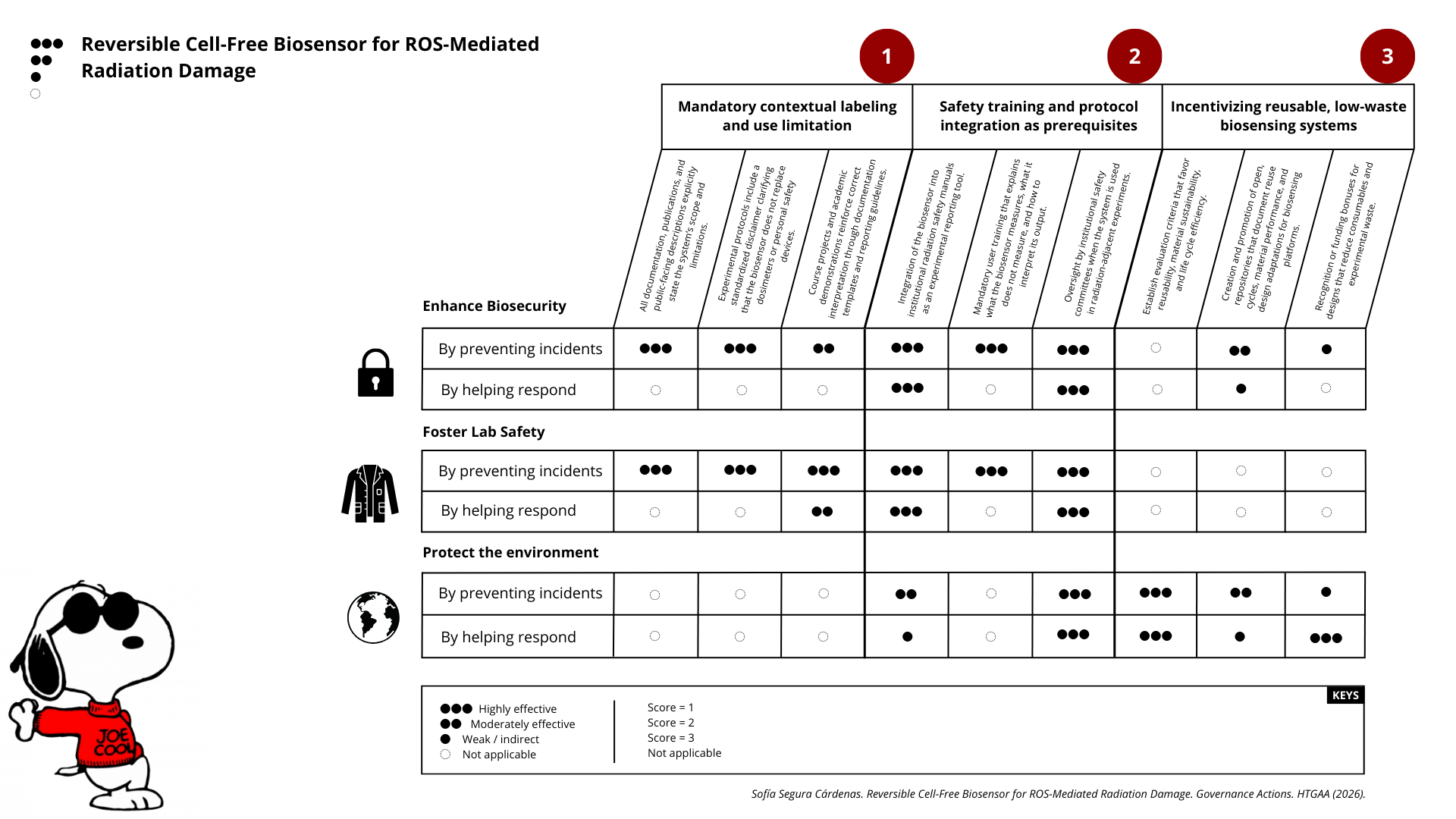
Next, score (from 1-3 with, 1 as the best, or n/a) each of your governance actions against your rubric of policy goals. The following is one framework but feel free to make your own:
Does the option:
Option 1
Option 2
Option 3
Enhance Biosecurity
• By preventing incidents
• By helping respond
Foster Lab Safety
• By preventing incident
• By helping respond
Protect the environment
• By preventing incidents
• By helping respond
Other considerations
• Minimizing costs and burdens to stakeholders
• Feasibility?
• Not impede research
• Promote constructive applications
Last, drawing upon this scoring, describe which governance option, or combination of options, you would prioritize, and why. Outline any trade-offs you considered as well as assumptions and uncertainties. For this, you can choose one or more relevant audiences for your recommendation, which could range from the very local (e.g. to MIT leadership or Cambridge Mayoral Office) to the national (e.g. to President Biden or the head of a Federal Agency) to the international (e.g. to the United Nations Office of the Secretary-General, or the leadership of a multinational firm or industry consortia). These could also be one of the “actor” groups in your matrix.
PART 1. FIXING THE COURSE
First, describe a biological engineering application or tool you want to develop and why. This could be inspired by an idea for your HTGAA class project and/or something for which you are already doing in your research, or something you are just curious about.
NOTE: This project is just the initial idea, it can be subjected to changes and upgrades in the near future.
Project: Reversible Cell-Free Biosensor for ROS-Mediated Radiation Damage
This project aims to design a reversible, cell-free biosensor capable of reporting radiation-induced oxidative damage through a visible biochemical signal.
The system is based on a DNA-programmed TX–TL circuit embedded within a hydrogel matrix, inspired by biological systems that can transition between active and inactive states under physical stress. Upon exposure to radiation-induced reactive oxygen species (ROS), the biosensor activates a transient fluorescent response, which gradually returns to a basal state once the stimulus is removed, enabling reuse of the material.
By decoupling damage sensing from living cells, this platform provides a controllable and modular approach to studying radiation effects on biological matter.
One-sentence project goal
The goal of this project is to engineer a reversible, reusable, cell-free biosensor that translates radiation-induced oxidative damage into a transient biochemical signal.
Background, application and why does it matter
The primary application of this biosensor is in radiation physics, medical physics and even space science, where it can be used as a reusable biological dosimetry platform to study oxidative damage induced by ionizing radiation.
Rather than measuring radiation directly, the system reports biologically relevant damage, specifically ROS generation, offering insight into how physical radiation translates into molecular stress in biological systems. This makes the material particularly valuable for experimental radiation setups, calibration studies, and comparative stress assays, without the need for living models.
The material functions as a reversible biological stress reporter. Instead of permanently activating or degrading under radiation-induced stress, it temporarily switches state to signal damage and then returns to baseline, enabling repeated use and long-term monitoring.
In medical physics and radiobiology, many existing sensing systems present fundamental limitations:
They degrade over time
They saturate under high stimulus
They are single-use
They cannot be reset or recovered
Similarly, most biological sensors:
lose viability
or remain irreversibly activated after damage
This creates a gap between physical radiation sensing and biologically meaningful damage reporting. The hydrogel is not just a container. While individual stress-responsive genetic elements are well characterized, their integration into a reusable, reversible cell-free biomaterial capable of multiple stress-response cycles remains largely unexplored.
Inspiration
The project is inspired by simple biological systems, such as jellyfish, which exhibit functional resilience and reversible state transitions despite minimal organizational complexity. These organisms demonstrate that biological function does not always require permanent activation or structural complexity, but can instead rely on transient, physics-driven responses to environmental stress.
Translating this principle into a synthetic, cell-free context, the proposed biosensor explores how biological states—such as gene expression and signal emission—can be reversibly triggered by physical damage and allowed to relax back to a stable baseline.
What makes this a synthetic biology project
This project constitutes a synthetic biology approach by designing and programming a DNA-based TX–TL circuit that links oxidative stress sensing to a controlled biochemical output to manifest a visible fluorescent signal. The circuit architecture, combined with material constraints imposed by the hydrogel matrix, enables tunable activation, decay, and reversibility of the signal.
Signal intensity correlates with stress magnitude, while signal reversibility reflects the system’s ability to recover to a baseline state. System reversibility is achieved through the co-design of a stress-responsive genetic circuit and a diffusion-regulated material matrix, enabling transient activation and passive return to a basal state without permanent system alteration. The system does not shut down because it fails; it shuts down because it is designed to relax back to its original state.
This platform is thinked to be modular, allowing future expansion to additional damage types. Rather than engineering a new organism, the project focuses on engineering biological function, emphasizing control, modularity, and reusability.
Conceptual state transition
The system starts in an OFF (basal) state
Oxidative stress is applied (e.g. H₂O₂ or radiation-induced ROS)
The system enters a “damage state”
A fluorescent signal is activated
The stress is removed
The system relaxes back to its basal state
Engineering design decisions
Biological Circuit Controls
Material (Hydrogel) Controls
What is detected (ROS, damage, stress)
How much stimulus enters the system
What signal is produced (fluorescence)
How fast the stimulus diffuses
Activation threshold and sensitivity
How long the stimulus is retained
Timing of signal initiation
Rate of stimulus clearance
Duration of protein expression
Smoothness of system shutdown
Signal termination mechanisms
Buffering of damage spikes
Susceptibility to noise or false positives
Protection of TX–TL components
Key tunable parameters in the system design include:
duration of protein expression
protein degradation rate
response speed
energy consumption
lifetime of the TX–TL system
Primary and secondary reporting strategy
Primary signal: fluorescence intensity
Secondary signal: temporal dynamics of activation and decay
Interpretation:
Fluorescence intensity reflects the magnitude of ROS-induced damage
Signal duration and decay profile reflect the dynamic response of the system under stress
Simplifying
How much it glows → magnitud of the damage How fast it starts glowing → intensity of the stress How the signal declines → dynamics of the system under damage
Reversibility is not interpreted as a property of the damage itself, but as a designed feature of the biosensor, enabling repeated use under multiple damage cycles.
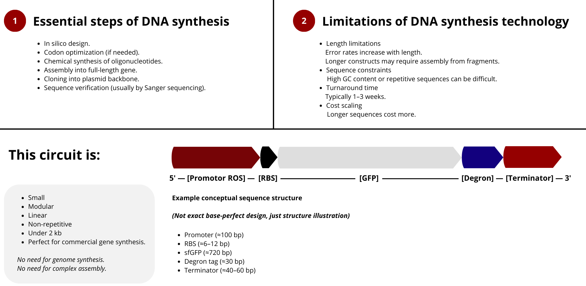
Circuit architecture
[ROS-sensitive promoter] ↓ [Fluorescent protein + degron] ↓ [Terminator]
Why this is non-trivial (and why it’s innovative)
Poor design choices lead to failure modes such as:
Gel too dense → stimulus never reaches the circuit → no activation
Gel too loose → excessive activation → no shutdown
Reporter too stable → permanent signal → no reuse
Circuit too sensitive → noise and false positives
PART 2. PROJECT CONSIDERATIONS
Next, describe one or more governance/policy goals related to ensuring that this application or tool contributes to an “ethical” future, like ensuring non-malfeasance (preventing harm). Break big goals down into two or more specific sub-goals. Below is one example framework (developed in the context of synthetic genomics) you can choose to use or adapt, or you can develop your own. The example was developed to consider policy goals of ensuring safety and security, alongside other goals, like promoting constructive uses, but you could propose other goals for example, those relating to equity or autonomy.
Governance and Policy Considerations
flowchart TB
    G["Governance & Policy Goals"]

    G --> A["Non-malfeasance<br/>(Preventing Harm)"]
    A --> A1["Cell-free TX–TL limits dual-use potential"]
    A --> A2["Avoids human or clinical deployment"]
    A --> A3["Environment friendly"]

    G --> B["Safe and Responsible Research"]
    B --> B1["Transparency in system limitations"]
    B --> B2["Reproducibility and containment"]
    B --> B3["Ensuring personal safety and capacitation"]
    B --> B4["Financial responsability"]

    G --> C["Constructive & Equitable Use"]
    C --> C1["Accessibility of the platform"]
    C --> C2["Supports education and interdisciplinary research"]
    C --> C3["Promotion of heuristic rules/method"]
• The biosensor is designed as a cell-free system, preventing replication, evolution, or environmental persistence, thereby reducing biosafety and biosecurity risks.
Sub-Goal 2A. Avoids human or clinical deployment
• The system is not intended for in vivo, clinical, or diagnostic use; clear communication of this limitation helps prevent inappropriate application and fends emerging ethical concerns about animal and human clinical trials.
Sub-Goal 3A. Environment friendly
• This project prioritizes environmentally responsible design by relying on hydrogel matrices derived from biodegradable, bio-based, or naturally sourced polymers. Such materials are often obtained from renewable resources or industrial by-products, reducing environmental impact compared to synthetic, non-degradable sensing technologies. Additionally, the reusability of the biosensor minimizes material waste and lowers the frequency of disposal, contributing to a more sustainable experimental practice.
Sub-Goal 1B. Transparency in system limitations
• The biosensor reports oxidative damage via ROS signaling rather than direct radiation dose, and this distinction must be clearly stated to avoid misinterpretation.
Sub-Goal 2B. Reproducibility and containment
• The use of in silico circuit design and controlled TX–TL systems improves reproducibility while minimizing unintended biological interactions.
Sub-Goal 3B. Ensuring personal welfare and capacitation
• Because the system is intended for studying radiation-induced damage in controlled environments, its use must be accompanied by appropriate safety protocols and user training. This biosensor is explicitly not designed to replace personal dosimeters or occupational safety monitoring devices. Clear operational guidelines, radiation-handling protocols, and user capacitation are required to ensure that the biosensor is employed strictly as an experimental tool, without increasing risk to personnel.
Sub-Goal 4B. Financial responsability
• The proposed system emphasizes cost-effective design through the use of low-cost materials, minimal infrastructure requirements, and a reusable sensing strategy. By enabling multiple experimental cycles within the same biosensor material, the system reduces recurring expenses associated with single-use sensors or consumables. This extended operational lifetime represents a significant financial advantage for laboratories and institutions, supporting responsible allocation of economic resources.
Sub-Goal 1C. Accessibility of the platform
• Cell-free and hydrogel-based systems lower infrastructure barriers, making the platform more accessible to educational and research laboratories.
Sub-Goal 2C. Supports education and interdisciplinary research
• The project bridges synthetic biology, materials science, and medical physics while maintaining clear ethical boundaries around scope and use.
Sub-Goal 3C. Promotion of heuristic rules
• This project adopts a heuristic-driven design philosophy, leveraging simple, interpretable rules to guide system construction and experimentation. Material properties, circuit dynamics, and experimental steps are intentionally ordered to maximize efficiency—favoring low-cost, low-complexity processes early and reserving more resource-intensive steps for later stages. This approach improves time efficiency, reduces unnecessary expenditures, and promotes accessible, transferable design strategies that can be adapted across laboratories and disciplines.
PART 3. THE WHO AND THE HOW
Next, describe at least three different potential governance “actions” by considering the four aspects below (Purpose, Design, Assumptions, Risks of Failure & “Success”). Try to outline a mix of actions (e.g. a new requirement/rule, incentive, or technical strategy) pursued by different “actors” (e.g. academic researchers, companies, federal regulators, law enforcement, etc). Draw upon your existing knowledge and a little additional digging, and feel free to use analogies to other domains (e.g. 3D printing, drones, financial systems, etc.).
Example
Purpose: What is done now and what changes are you proposing?
Design: What is needed to make it “work”? (including the actor(s) involved - who must opt-in, fund, approve, or implement, etc)
Assumptions: What could you have wrong (incorrect assumptions, uncertainties)?
Risks of Failure & “Success”: How might this fail, including any unintended consequences of the “success” of your proposed actions?
Governance Action 1 — Mandatory contextual labeling and use limitation
Actor(s): Academic researchers, research institutions, funding agencies.
Purpose
Currently, biosensors designed for radiation-related applications can be misinterpreted as direct radiation detectors or clinical tools. This project proposes a mandatory contextual labeling requirement stating that the system detects ROS-mediated damage, not radiation dose, and is intended strictly for in vitro experimental use. The change ensures that the tool is not misapplied in clinical, occupational, or regulatory contexts.
Design
To make this work, institutions and funding bodies would require that:
All documentation, publications, and public-facing descriptions explicitly state the system’s scope and limitations.
Experimental protocols include a standardized disclaimer clarifying that the biosensor does not replace dosimeters or personal safety devices.
Course projects and academic demonstrations reinforce correct interpretation through documentation templates and reporting guidelines.
Assumptions
This action assumes that misinterpretation is a primary pathway for harm and that clear documentation meaningfully influences user behavior. It also assumes that researchers and students will comply with labeling norms when they are formally required.
Risks of Failure & “Success”
Failure risk: Labels may be ignored, especially when the system performs well and appears “sensor-like.”
Risk of success: If widely adopted, the tool could become a de facto standard for damage reporting, tempting users to extend it beyond its intended domain without appropriate validation.
Governance Action 2 — Safety training and protocol integration as a prerequisite for use
Actor(s): Research institutions, laboratory safety committees, instructors.
Purpose
Radiation-related experimentation already requires specialized training, but novel biosensors can create a false sense of safety. This action proposes that use of the biosensor be explicitly tied to existing radiation safety training and protocols, reinforcing that the tool supplements—but does not replace—established safety infrastructure.
Design
This action would require:
Integration of the biosensor into institutional radiation safety manuals as an experimental reporting tool.
Mandatory user training that explains what the biosensor measures, what it does not measure, and how to interpret its output.
Oversight by institutional safety committees when the system is used in radiation-adjacent experiments.
Assumptions
This approach assumes that institutions already have safety frameworks capable of absorbing new tools, and that users are more likely to behave responsibly when a technology is embedded within formal safety structures.
Risks of Failure & “Success”
Failure risk: Training could become procedural rather than substantive, reducing its effectiveness.
Risk of success: If the biosensor becomes normalized within safety workflows, it may be incorrectly perceived as an authoritative indicator of safety rather than an experimental proxy.
Governance Action 3 — Incentivizing reusable, low-waste biosensing systems
Actor(s): Funding agencies, academic programs, sustainability-focused research initiatives.
Purpose
Many sensing technologies are single-use, expensive, or environmentally burdensome. This action proposes incentivizing reusable and low-waste biosensor designs, positioning reusability and material efficiency as desirable research outcomes rather than secondary considerations.
Design
This could be implemented through:
Establish evaluation criteria that favor reusability, material sustainability, and life cycle efficiency.
Creation and promotion of open, repositories that document reuse cycles, material performance, and design adaptations for biosensing platforms.
Recognition or funding bonuses for designs that reduce consumables and experimental waste.
Assumptions
This action assumes that researchers respond to incentive structures and that sustainability metrics can be meaningfully evaluated without stifling innovation or creativity.
Risks of Failure & “Success”
Failure risk: Incentives may encourage superficial reuse claims without rigorous validation.
Risk of success: Strong emphasis on reuse could discourage exploration of necessary single-use or high-sensitivity designs in certain contexts.
PART 4. HOW WELL DO YOU DO?
Next, score (from 1-3 with, 1 as the best, or n/a) each of your governance actions against your rubric of policy goals.
PART 5. PRIORITIES
Last, drawing upon this scoring, describe which governance option, or combination of options, you would prioritize, and why. Outline any trade-offs you considered as well as assumptions and uncertainties. For this, you can choose one or more relevant audiences for your recommendation, which could range from the very local (e.g. to MIT leadership or Cambridge Mayoral Office) to the national (e.g. to President Biden or the head of a Federal Agency) to the international (e.g. to the United Nations Office of the Secretary-General, or the leadership of a multinational firm or industry consortia). These could also be one of the “actor” groups in your matrix.
Prioritized governance strategy and rationale
Drawing upon the governance scoring matrix, the most effective strategy for guiding the responsible development and use of the proposed reversible cell-free biosensor is a combined prioritization of Governance Options 1 and 2, with Governance Option 3 acting as a reinforcing, longer-term incentive mechanism.
Primary priority: Governance Options 1 and 2 (combined)
Option 1 — Mandatory contextual labeling and use limitation
+
Option 2 — Safety training and protocol integration as prerequisites
These two options consistently score highest across biosafety, lab safety, and environmental protection, particularly in their ability to prevent incidents rather than merely respond to them. Together, they address the most immediate risks associated with misuse, misinterpretation, or inappropriate deployment of the biosensor.
Option 1 ensures that the system is clearly framed as:
A cell-free, non-replicative biosensing platform
Not a personal radiation dosimeter
Not intended for clinical or in vivo use
This directly reduces the risk of over-interpretation of fluorescence signals and prevents the technology from being deployed outside its validated scope.
Option 2 complements this by embedding the biosensor within existing institutional safety cultures, requiring that users receive appropriate training in:
Radiation handling protocols
Interpretation of indirect ROS-based signals
Limitations of TX–TL systems
Importantly, this option does not introduce new regulatory burdens but instead leverages existing laboratory training and approval workflows, making it both feasible and scalable.
Trade-off considered:
These measures may slow early adoption or increase onboarding time for new users. However, this is outweighed by the reduction in misuse risk and the preservation of trust in the technology.
Option 3 — Incentivizing reusable, low-waste biosensing systems
While Option 3 scores lower in immediate incident prevention, it plays a crucial role in shaping long-term research behavior and system design choices. Incentives that reward reusability, lifecycle efficiency, and reduced consumables encourage adoption of the very properties that distinguish this biosensor from traditional single-use sensors.
Rather than acting as a primary safeguard, this option functions best as:
A structural reinforcement mechanism
+
A signal to researchers and institutions that sustainability and reuse are valued outcomes
Trade-off considered: Incentive-based mechanisms depend on institutional uptake and may have uneven effects across well-funded versus resource-limited laboratories. Their impact is therefore slower and less uniform than mandatory requirements.
Assumptions and Uncertainties
This prioritization assumes that:
Institutions and laboratories already possess baseline safety infrastructure
Users are willing to engage with training and labeling requirements
Regulatory bodies are receptive to non-single-use technologies
Uncertainties remain regarding:
How fluorescence-based damage reporting might be interpreted by non-experts
Variability in institutional enforcement of training standards
How incentive structures translate into real design decisions over time
Recommended audience
This governance strategy is primarily directed toward:
Institutional biosafety committees and laboratory leadership
Funding agencies and regulatory bodies overseeing research infrastructure
Organizations setting best-practice standards for cell-free and biosensing technologies
By acting at this institutional and regulatory level, the proposed governance combination balances safety, feasibility, innovation, and sustainability, aligning closely with the technical and ethical goals of the project.
WEEK 2 - LECTURE PREP
In preparation for Week 2’s lecture on “DNA Read, Write, and Edit," please review the follow materials
Lecture 2 slides as posted below.
The associated papers that are referenced in those slides. In addition, answer these questions in each faculty member’s section:
Homework Questions from Professor Jacobson: [Lecture 2 slides]
Nature’s machinery for copying DNA is called polymerase. What is the error rate of polymerase? How does this compare to the length of the human genome. How does biology deal with that discrepancy?
DNA Polymerase error rate and genome fidelity
DNA polymerase, the enzyme responsible for copying DNA during replication, has an intrinsic error rate of approximately 1 mistake per 10⁵ nucleotides incorporated.
The human genome contains about 3 × 10⁹ base pairs. At this raw error rate, tens of thousands of mutations would occur every time a human cell divides, which would be incompatible with life.
How biology addresses this discrepancy
Biological systems reduce replication errors through multiple layers of error correction:
Proofreading by DNA polymerase Many DNA polymerases possess 3′→5′ exonuclease activity, which allows them to remove incorrectly incorporated nucleotides immediately. This improves fidelity to roughly 1 error per 10⁷ nucleotides.
Post-replication mismatch repair (MMR) Additional cellular repair systems detect and correct mismatches that escape proofreading, further reducing the error rate to approximately 1 error per 10⁹–10¹⁰ nucleotides.
As a result, the final error rate is low enough that most cell divisions occur without introducing harmful mutations.
How many different ways are there to code (DNA nucleotide code) for an average human protein? In practice what are some of the reasons that all of these different codes don’t work to code for the protein of interest?
Coding Capacity of DNA for an Average Human Protein
An average human protein is approximately 300 amino acids long. Each amino acid is encoded by a codon, a sequence of three nucleotides.
Because there are 4 possible nucleotides (A, T, C, G), there are:
( 4^3 = 64 ) possible codons
Only 20 amino acids (plus stop signals)
This means the genetic code is degenerate, and most amino acids are encoded by multiple codons.
Number of Possible DNA Sequences for One Protein
If an average amino acid is encoded by ~3 synonymous codons, then the total number of possible DNA sequences that could encode a 300–amino acid protein is approximately:
[
3^{300}
]
This is an astronomically large number, meaning there are many distinct DNA sequences that can, in theory, encode the same protein.
Why Most Possible Codes Do Not Work in Practice
Despite this theoretical flexibility, not all synonymous DNA sequences function equally well due to several biological constraints:
Codon usage bias Organisms preferentially use certain codons over others. Rare codons can slow translation or cause ribosome stalling.
mRNA secondary structure Certain nucleotide sequences form stable secondary structures that hinder ribosome binding or elongation.
Translational accuracy and efficiency Codon choice can affect misincorporation rates and protein folding during translation.
Regulatory elements embedded in coding sequences Coding regions may overlap with regulatory signals affecting splicing, mRNA stability, or localization.
GC content and genome stability Extreme nucleotide compositions can impact DNA replication and transcription efficiency.
Because of these factors, only a small subset of all theoretically possible DNA sequences are biologically viable for producing a functional protein at appropriate levels.
Homework Questions from Dr. LeProust: [Lecture 2 slides]
What’s the most commonly used method for oligo synthesis currently?
The most commonly used method for oligonucleotide synthesis is solid-phase phosphoramidite chemistry. In this method, DNA is synthesized stepwise from the 3′ to the 5′ end on a solid support. Each cycle consists of four main steps: deprotection, coupling of a phosphoramidite nucleotide, capping of unreacted chains, and oxidation. This approach is highly automated, fast, and reliable, making it the standard technique used by commercial DNA synthesis providers.
Why is it difficult to make oligos longer than 200nt via direct synthesis?
It is difficult to synthesize oligos longer than ~200 nucleotides because errors accumulate with each synthesis cycle. Each nucleotide addition has a small but nonzero failure rate (incomplete coupling, side reactions, or deletions). As the oligo length increases, these errors compound exponentially, leading to a low fraction of full-length, correct sequences. Additionally, longer oligos are harder to purify effectively, since truncated products differ only slightly in length from the desired product.
Why can’t you make a 2000bp gene via direct oligo synthesis?
A 2000 bp gene cannot be made via direct oligo synthesis because the cumulative error rate would be extremely high, resulting in an almost negligible yield of error-free full-length DNA. Beyond error accumulation, chemical synthesis efficiency, purification limitations, and cost make direct synthesis impractical at this scale. Instead, long genes are constructed by assembling shorter, overlapping oligos using enzymatic methods such as PCR-based assembly or Gibson assembly, followed by cloning and sequence verification.
Homework Question from George Church: [Lecture 2 slides]
Choose ONE of the following three questions to answer; and please cite AI prompts or paper citations used, if any.
[Using Google & Prof. Church’s slide #4] What are the 10 essential amino acids in all animals and how does this affect your view of the “Lysine Contingency”?
The 10 essential amino acids in animals are those that cannot be synthesized de novo and therefore must be obtained from the diet:
Histidine
Isoleucine
Leucine
Lysine
Methionine
Phenylalanine
Threonine
Tryptophan
Valine
Arginine(essential in all animals during growth; in many adult animals it is conditionally essential)
How does this affect the view of the “Lysine Contingency”?
The “Lysine Contingency” refers to the idea that life—particularly animals—became evolutionarily dependent on lysine availability from external sources, because animals lost the ability to synthesize lysine. Since lysine is universally essential in animals and often limiting in plant-based diets (especially cereal grains), this creates a strong nutritional and evolutionary constraint.
This reinforces the view that the lysine contingency is real and biologically significant:
Animals are metabolically constrained by the loss of lysine biosynthesis pathways.
Ecosystems and food webs are shaped by lysine availability and by organisms (plants, fungi, bacteria) that can synthesize it.
It helps explain why lysine supplementation or biofortification (e.g., high-lysine crops) has a major impact on nutrition and health.
Overall, the universality of lysine as an essential amino acid in animals supports the idea that lysine availability is a key evolutionary and nutritional bottleneck rather than a trivial dietary detail.
Nguyen, P. Q., Soenksen, L. R., Donghia, N. M., Angenent-Mari, N. M., de Puig, H., Huang, A., Lee, R. A., Slomovic, S., Galbersanini, T., Lansberry, G., Sallum, H. M., Zhao, E. M., Niemi, J. B. & Collins, J. J. (2021). Wearable materials with embedded synthetic biology sensors for biomolecule detection. Nature Biotechnology, 39(11). https://doi.org/10.1038/s41587-021-00950-3
Karim, M. M. and Lasker, T. (2025). Electrochemical Biosensors for Cancer Biomarker Detection: Basic Concept, Design Strategy and Cutting‐Edge Development. Electrochemical Science Advances. https://doi.org/10.1002/elsa.70007
Liang, Q., Lu, Y. & Zhang, Q. (2022). Hydrogels‐Based Electronic Devices for Biosensing Applications. In Smart Stimuli-Responsive Polymers, Films, and Gels. https://doi.org/10.1002/9783527832385.ch10
Zhang, M., Xu, T., Liu, K., Zhu, L., Miao, C., Chen, T., Gao, M., Wang, J. & Si, C. (2024). Modulation and Mechanisms of Cellulose‐Based Hydrogels for Flexible Sensors. SusMat, 5. https://doi.org/10.1002/sus2.255
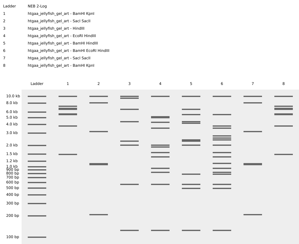
This week explores the read–write–edit toolkit: sequencing and synthesis workflows, restriction digests and gel electrophoresis, and early genome-editing frameworks.
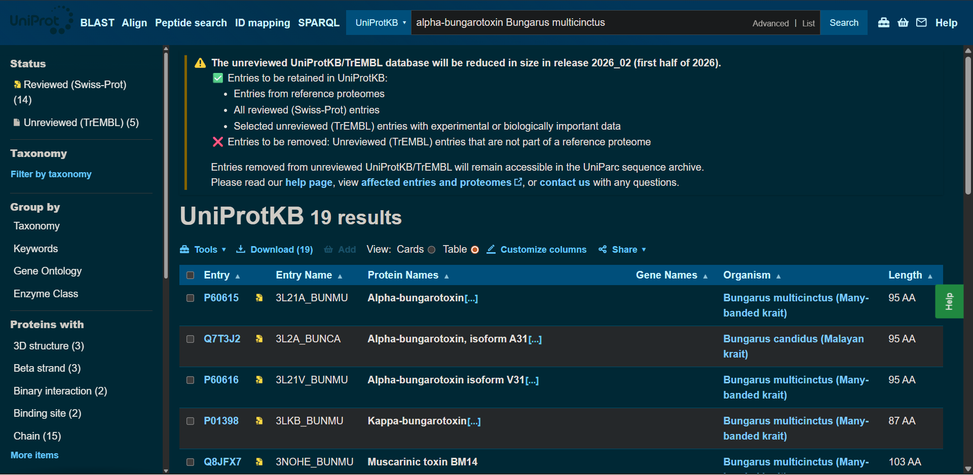
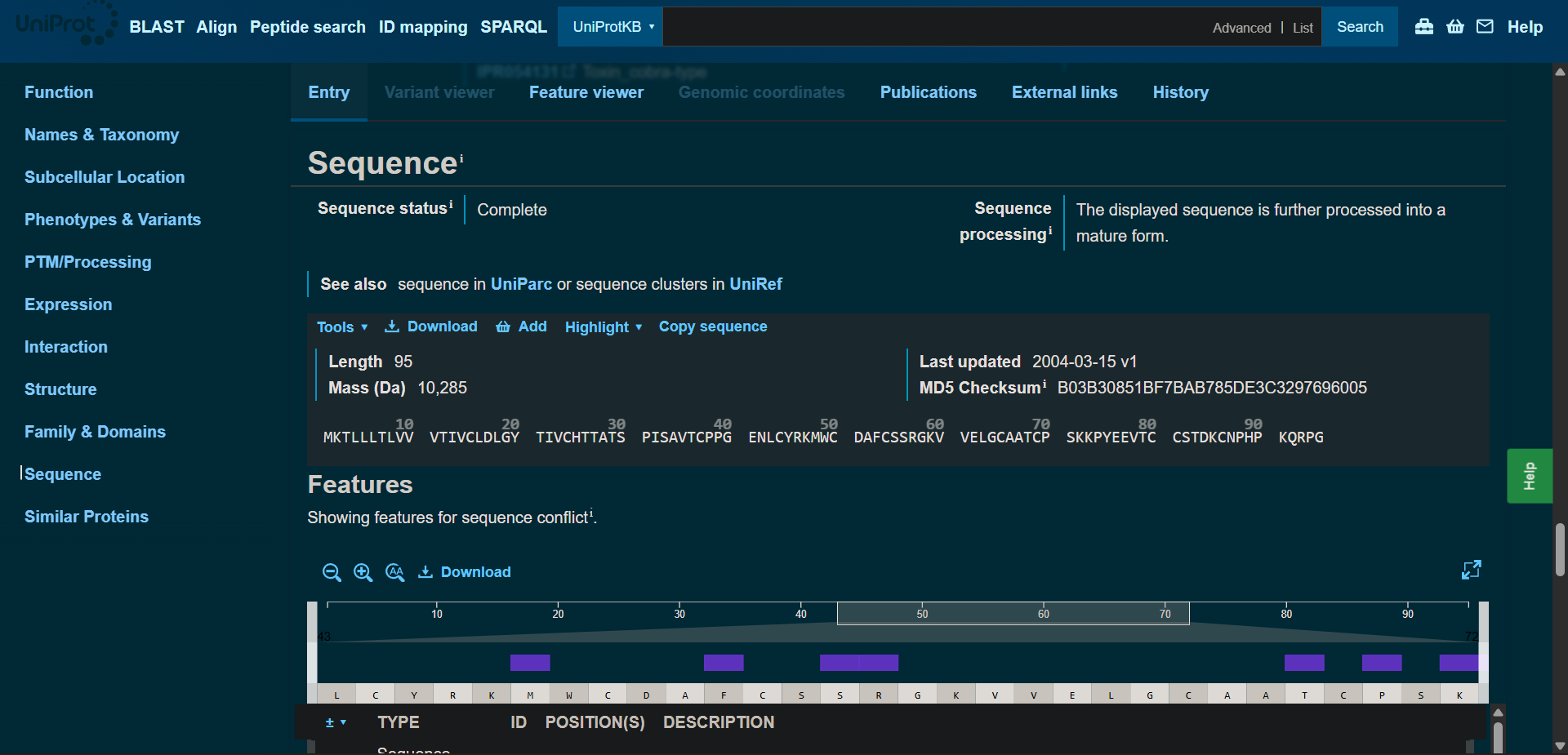
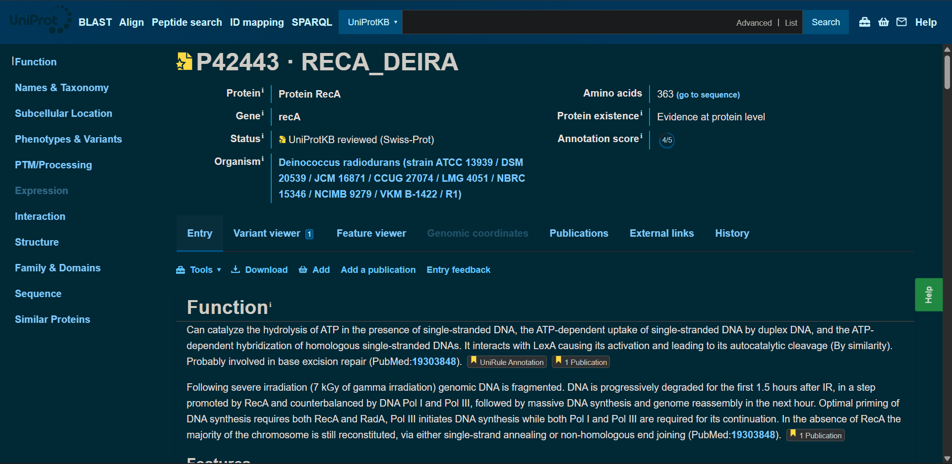
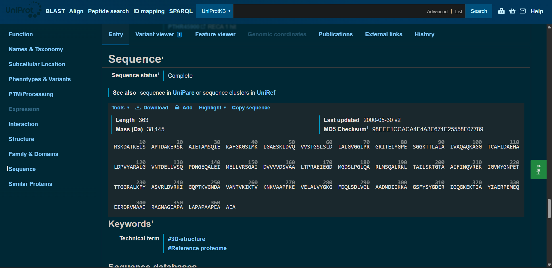
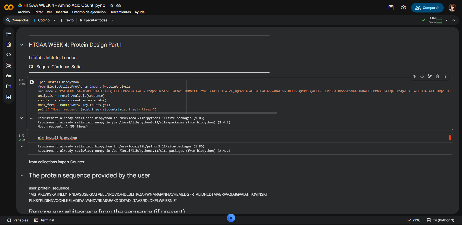
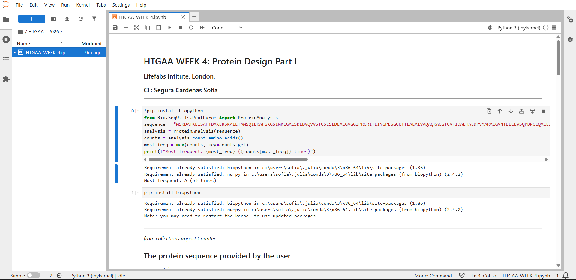
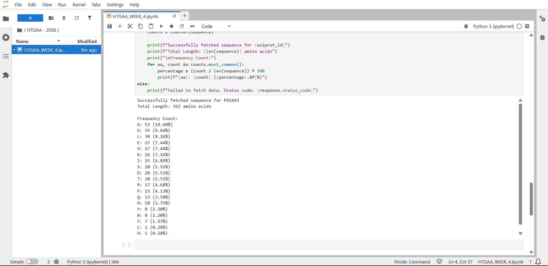
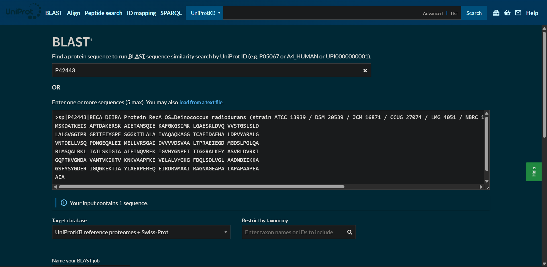
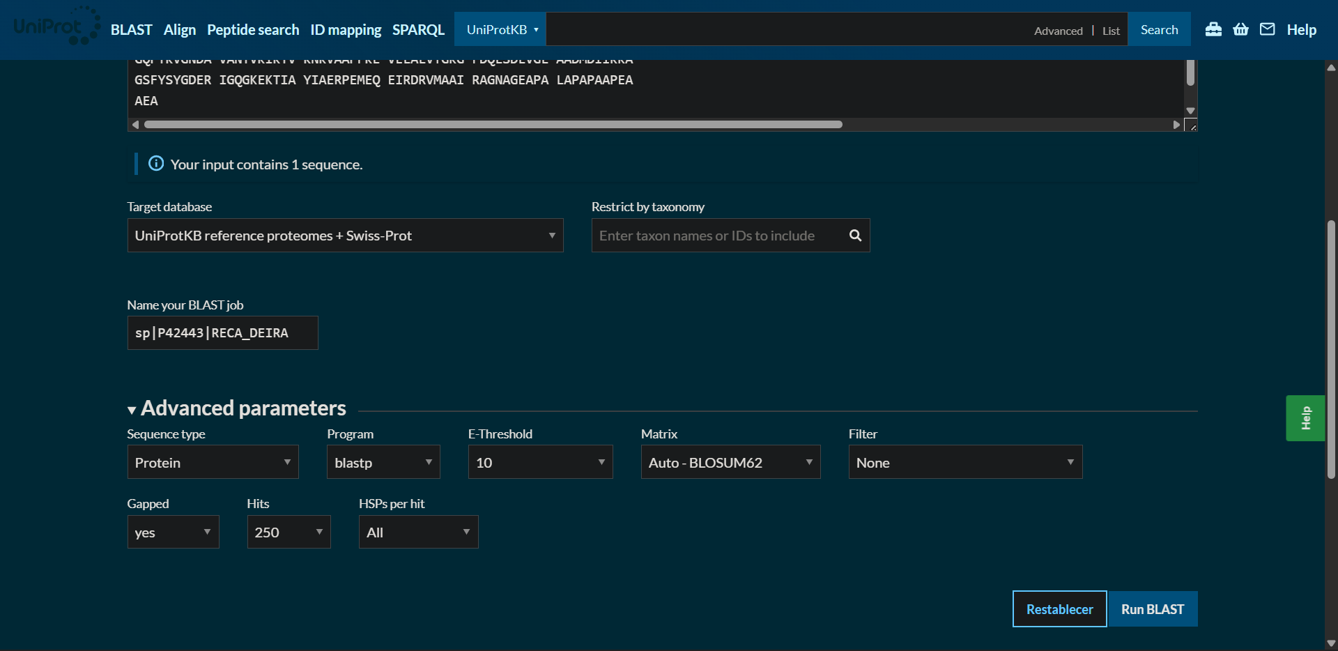
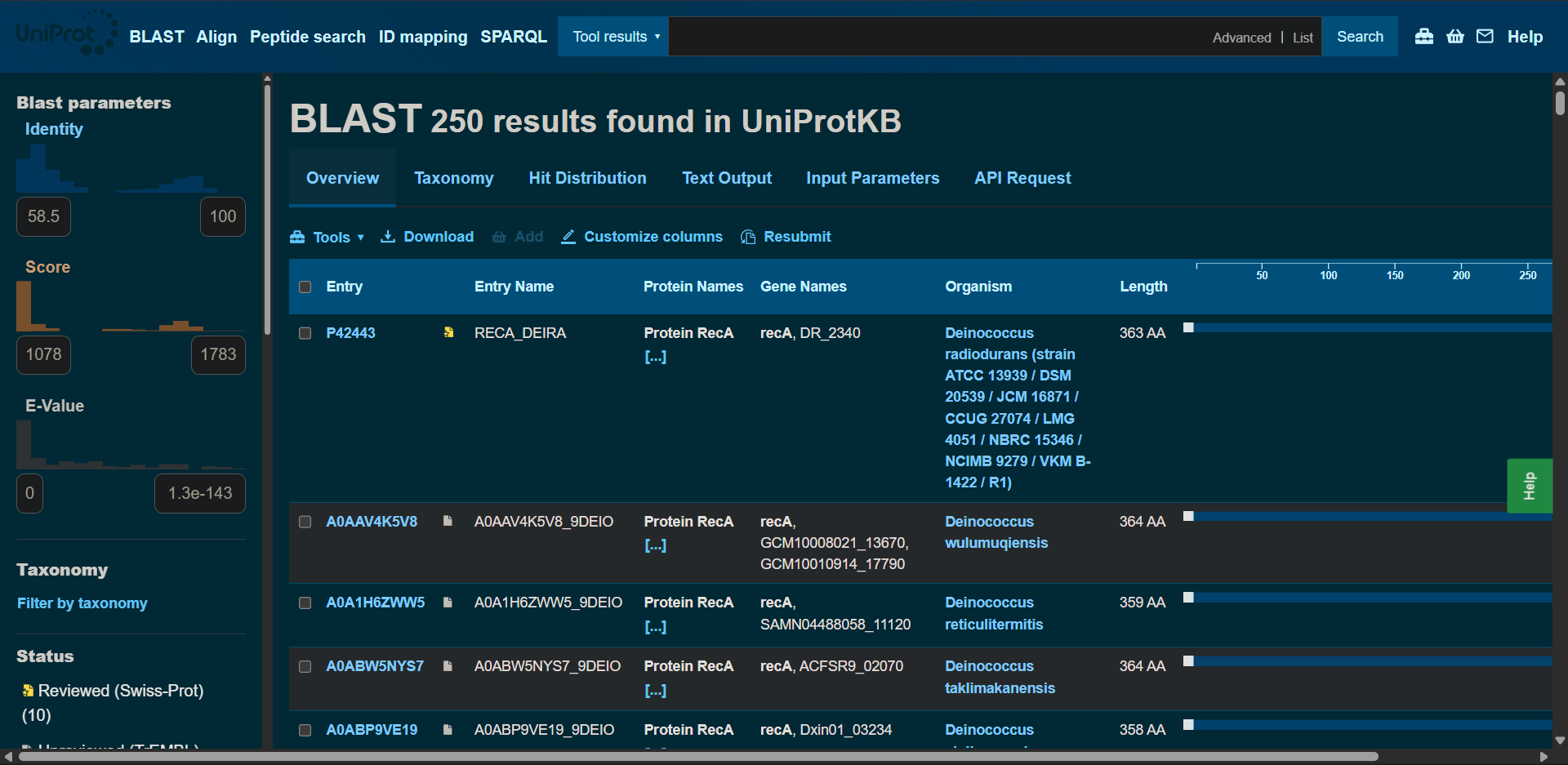
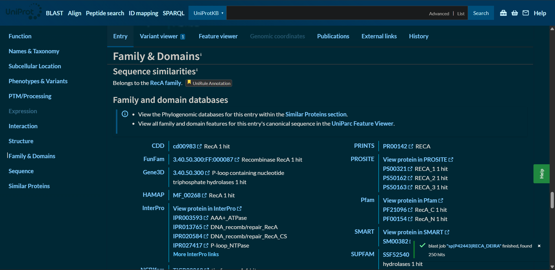
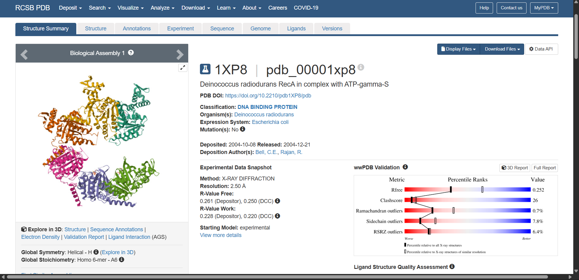
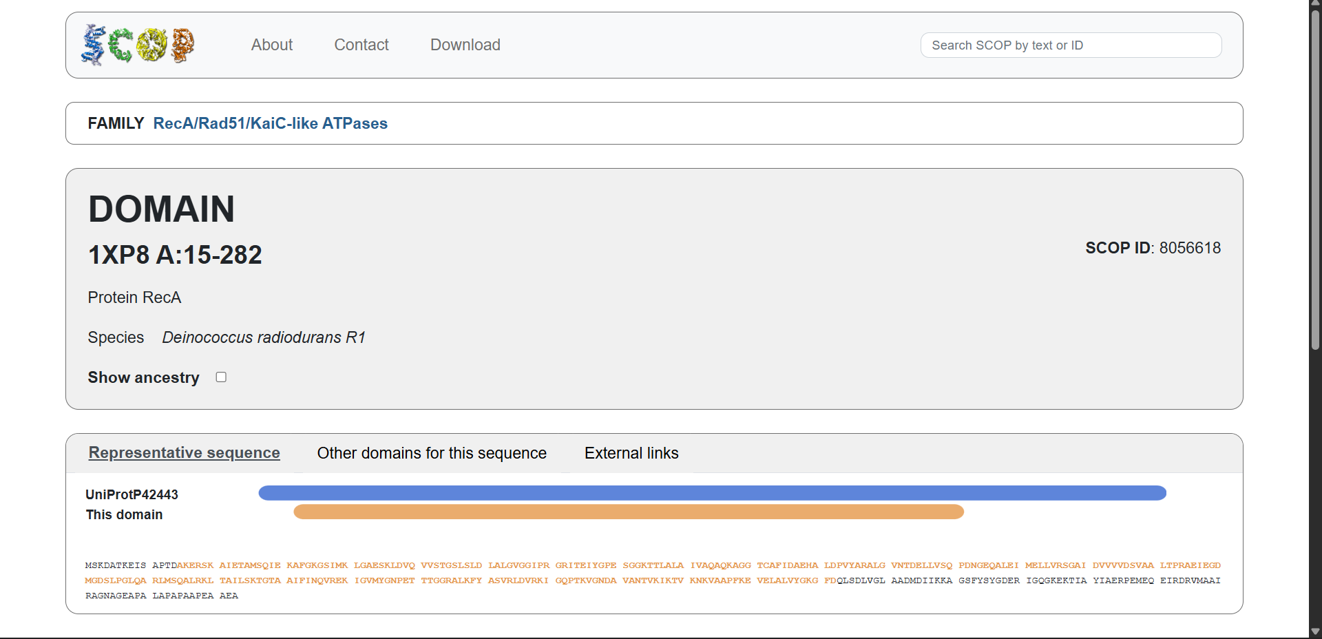
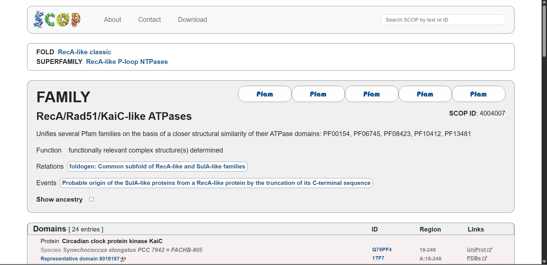
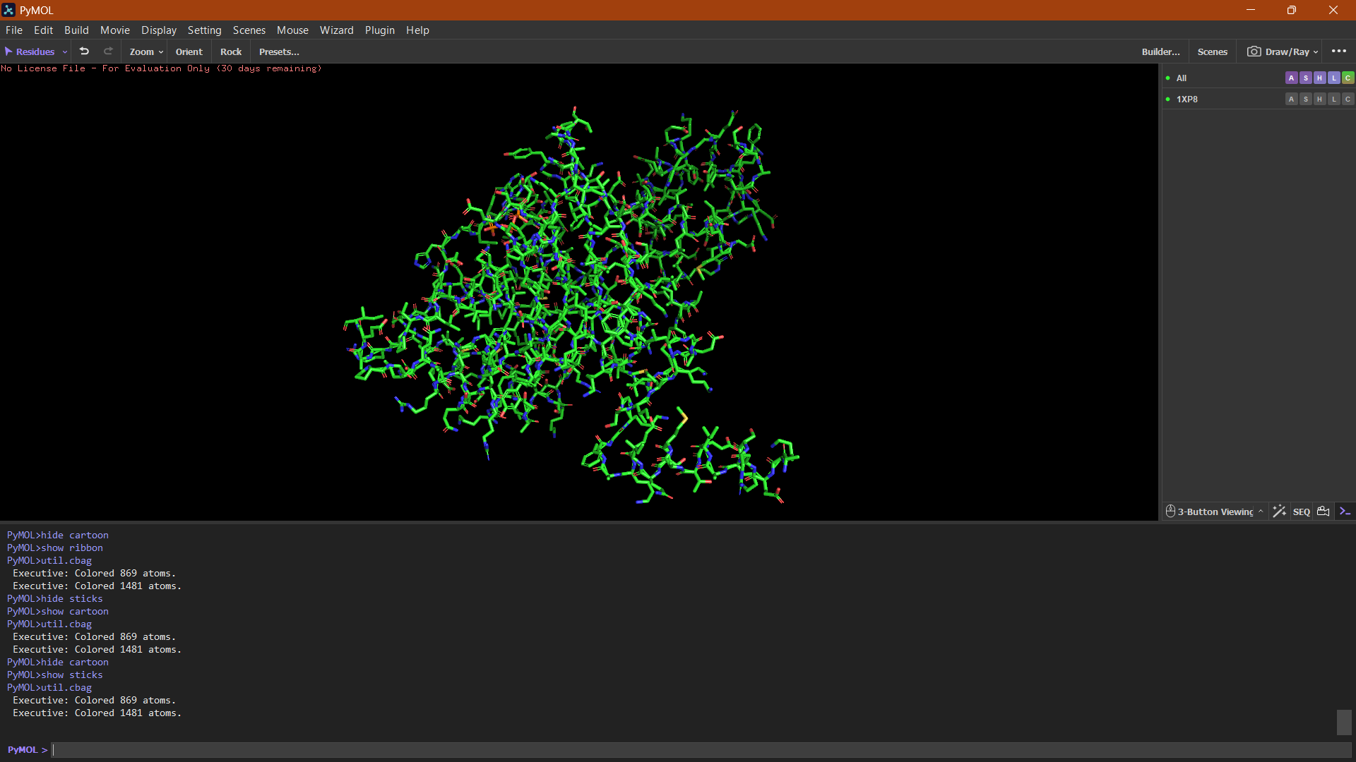
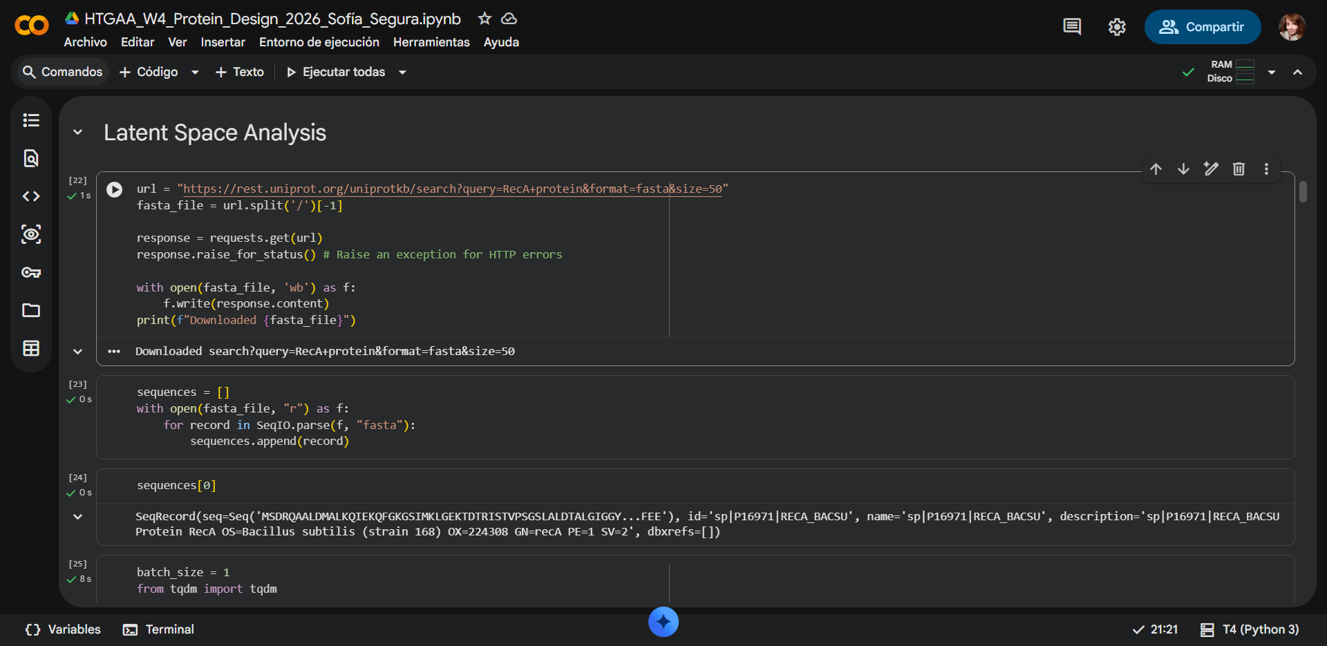
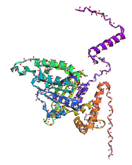
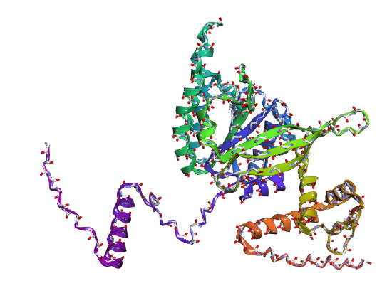
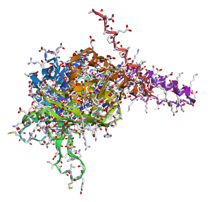
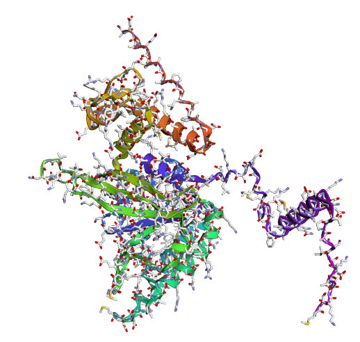
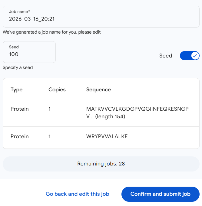
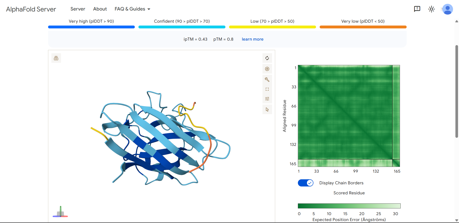
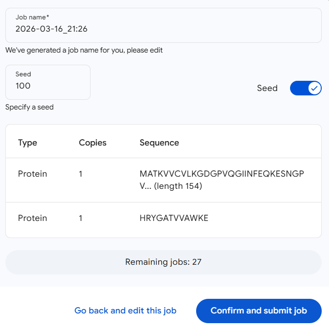
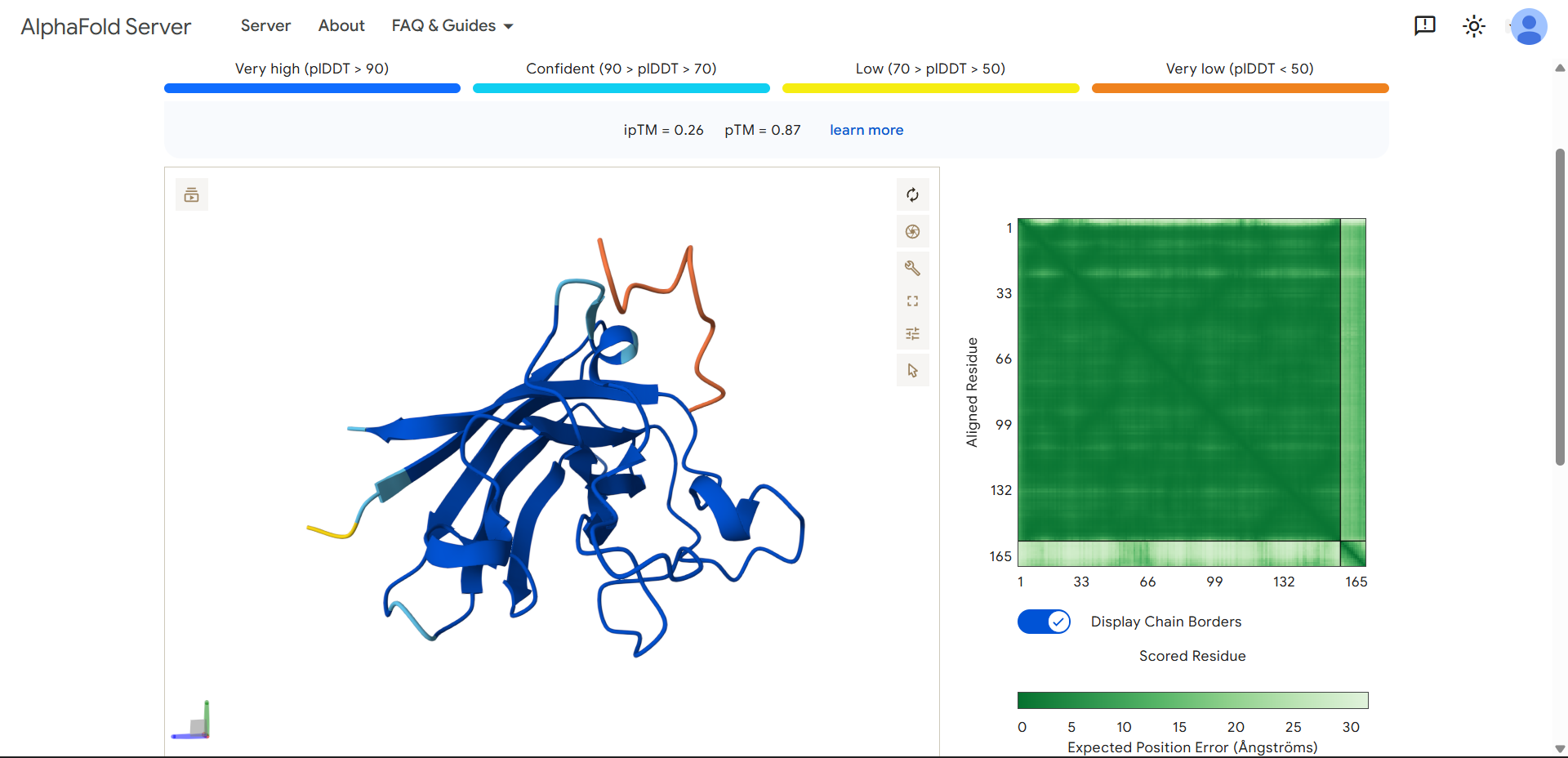
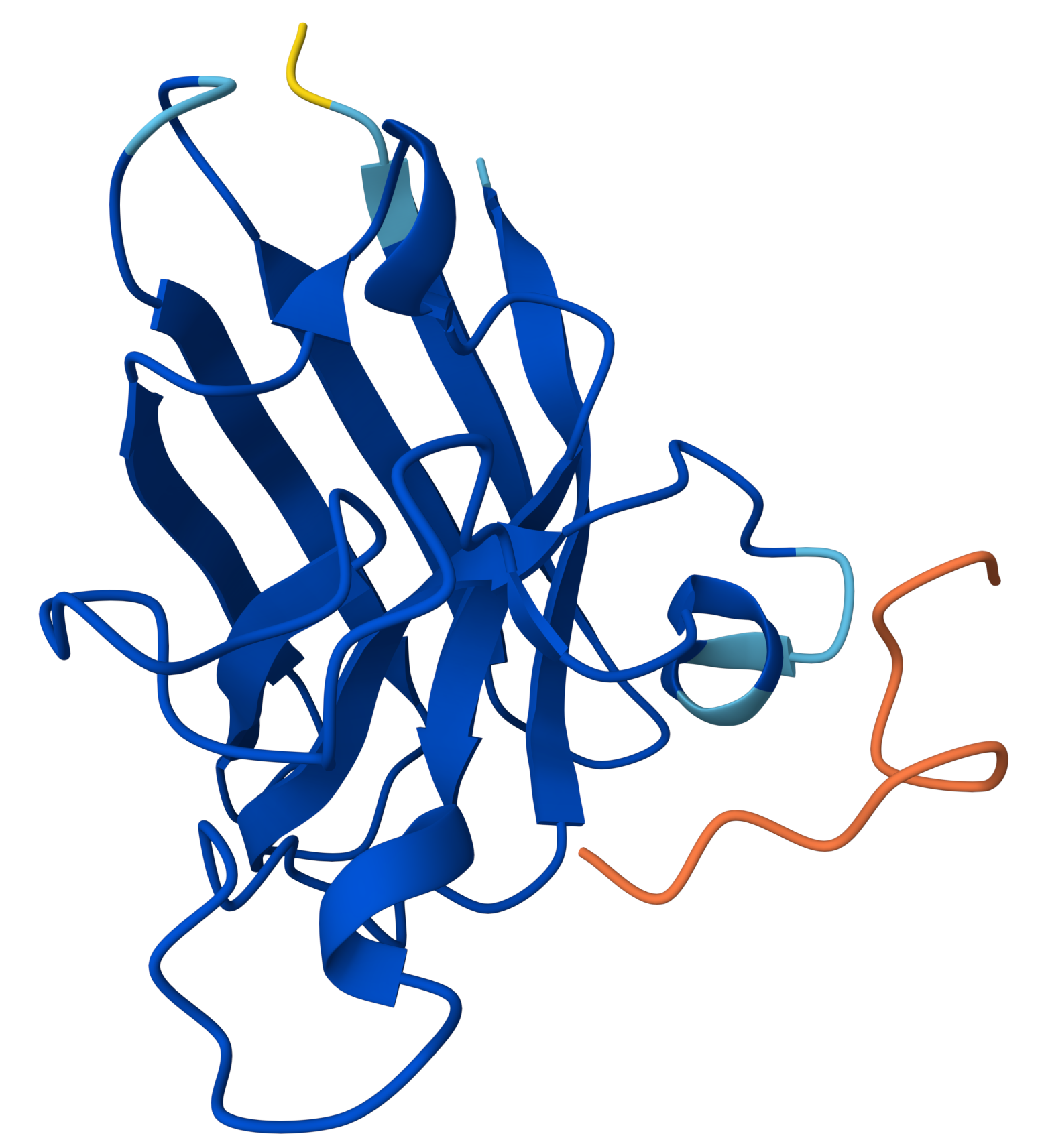
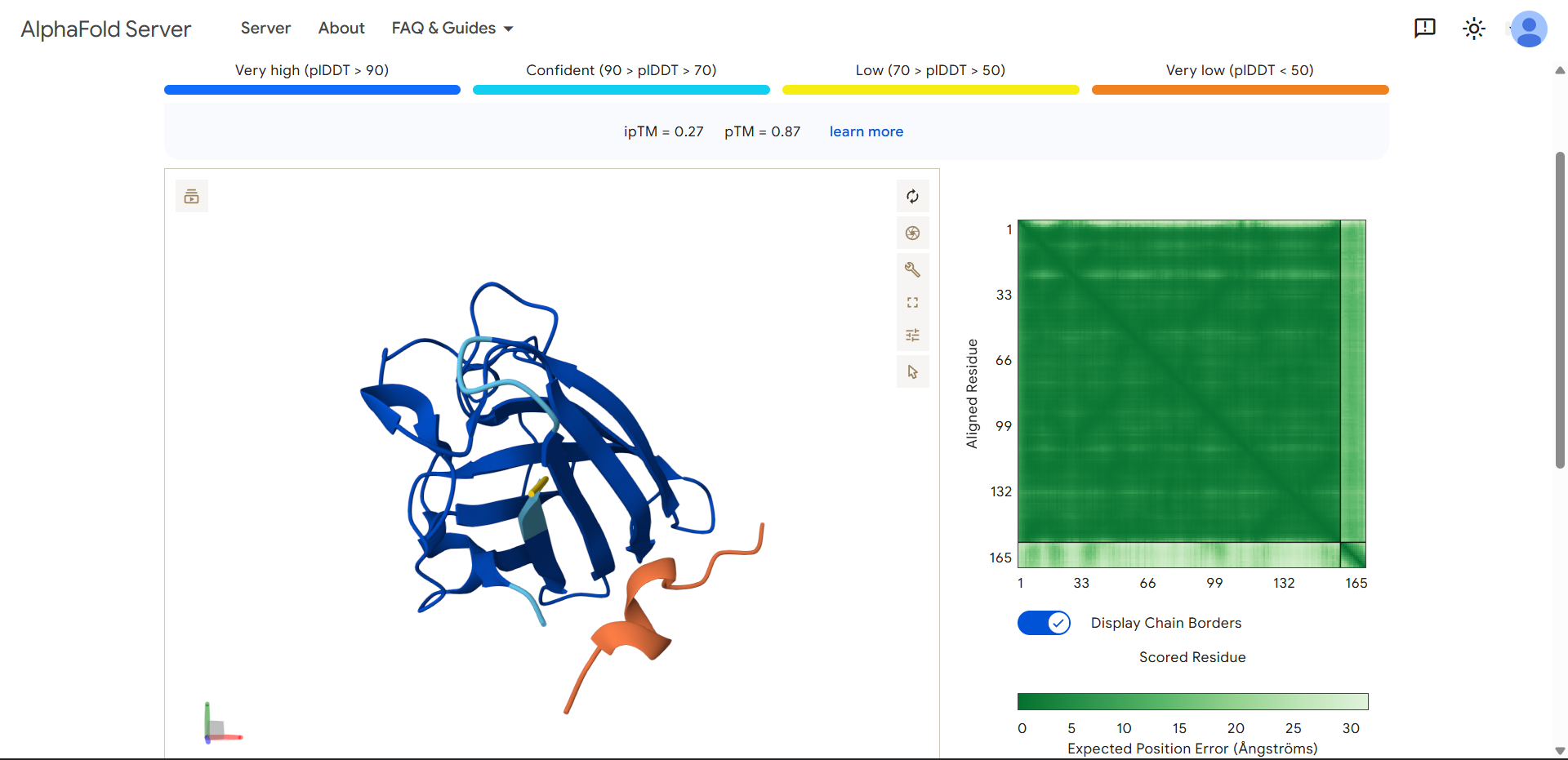
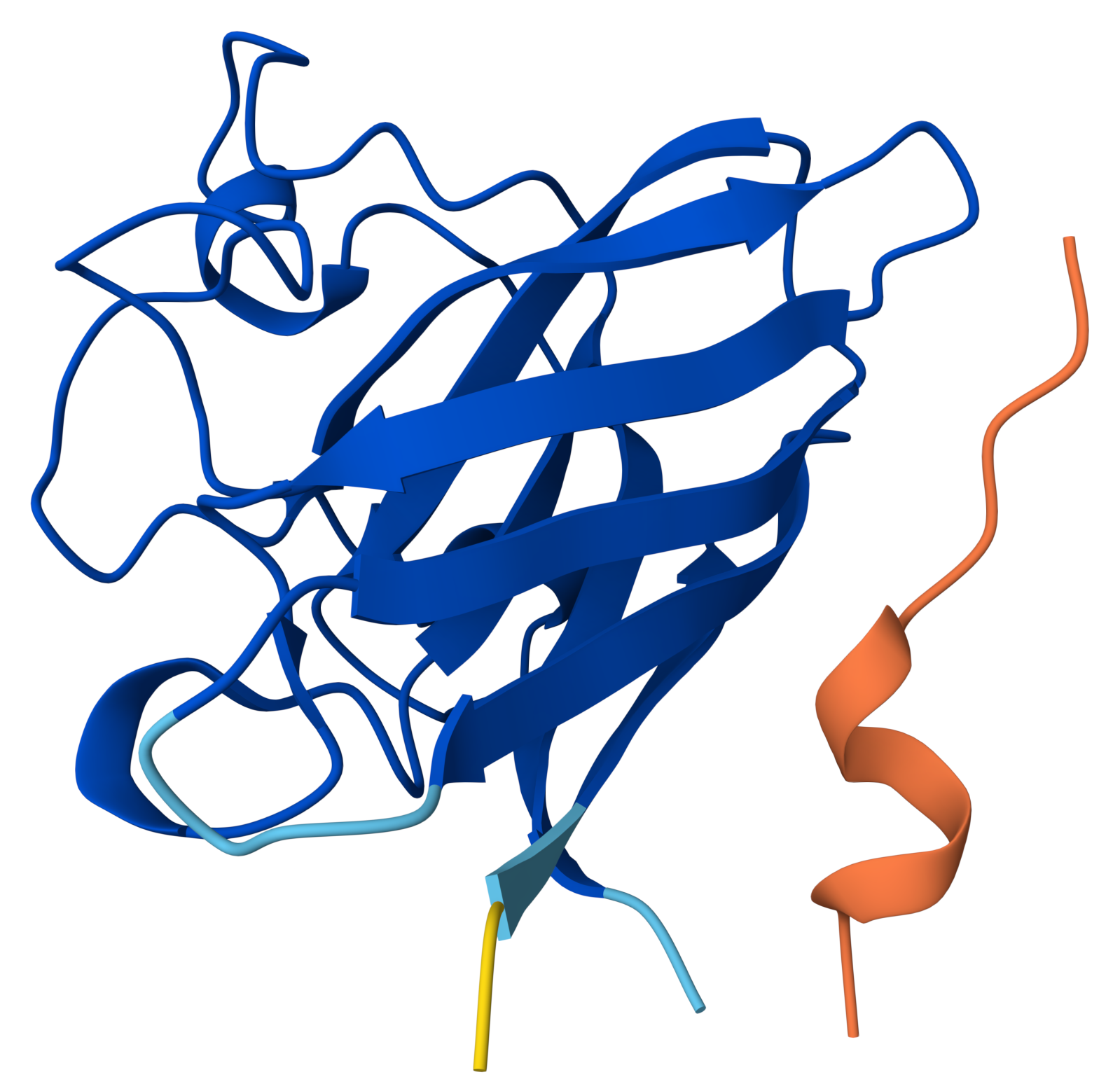
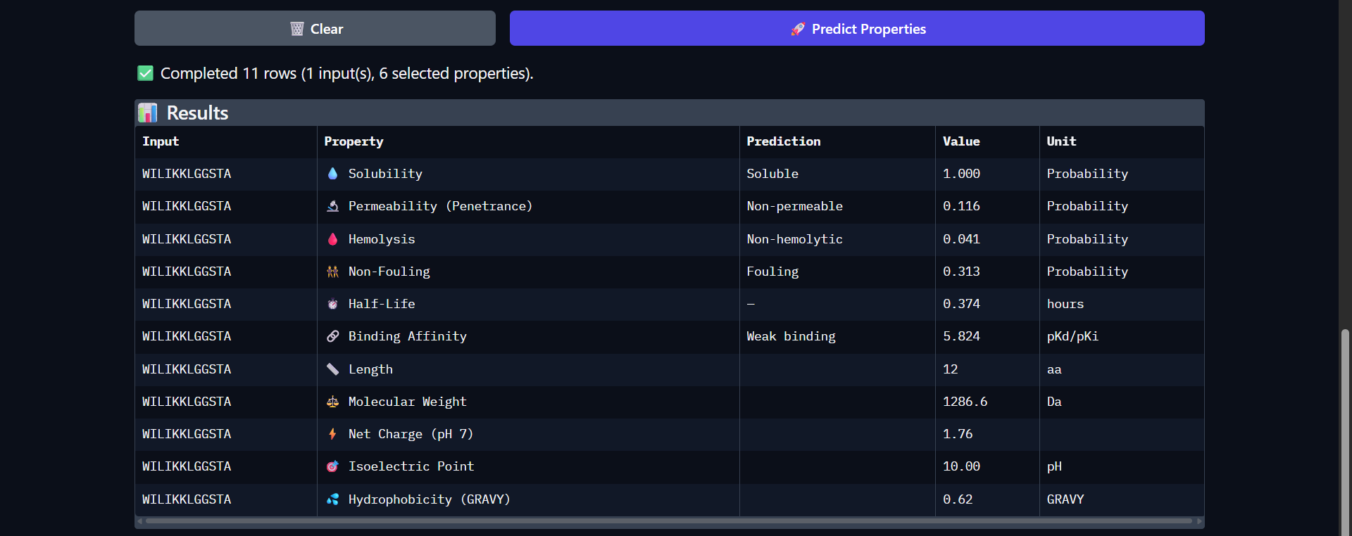
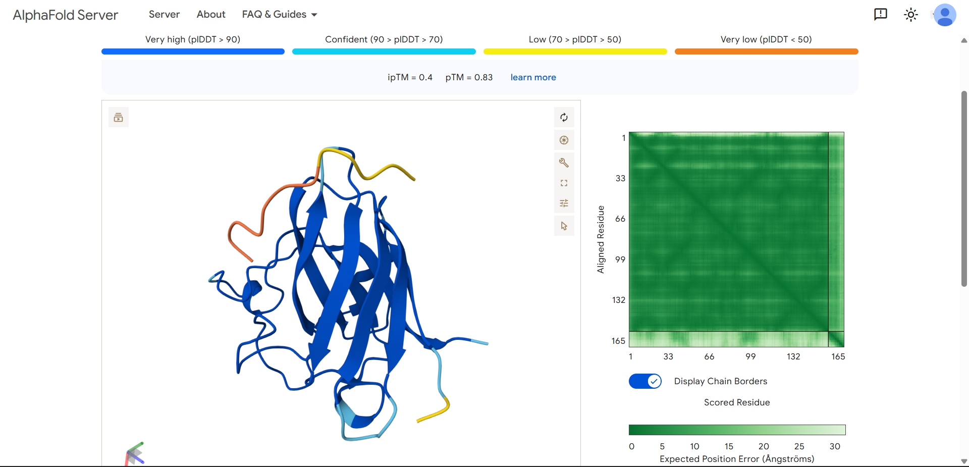
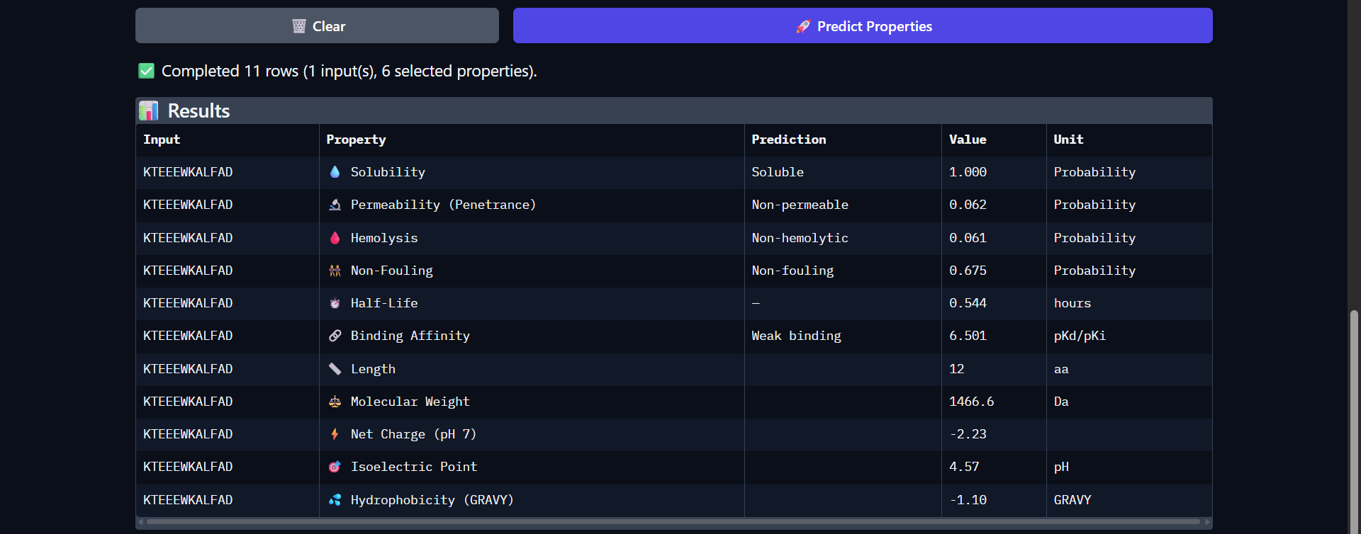
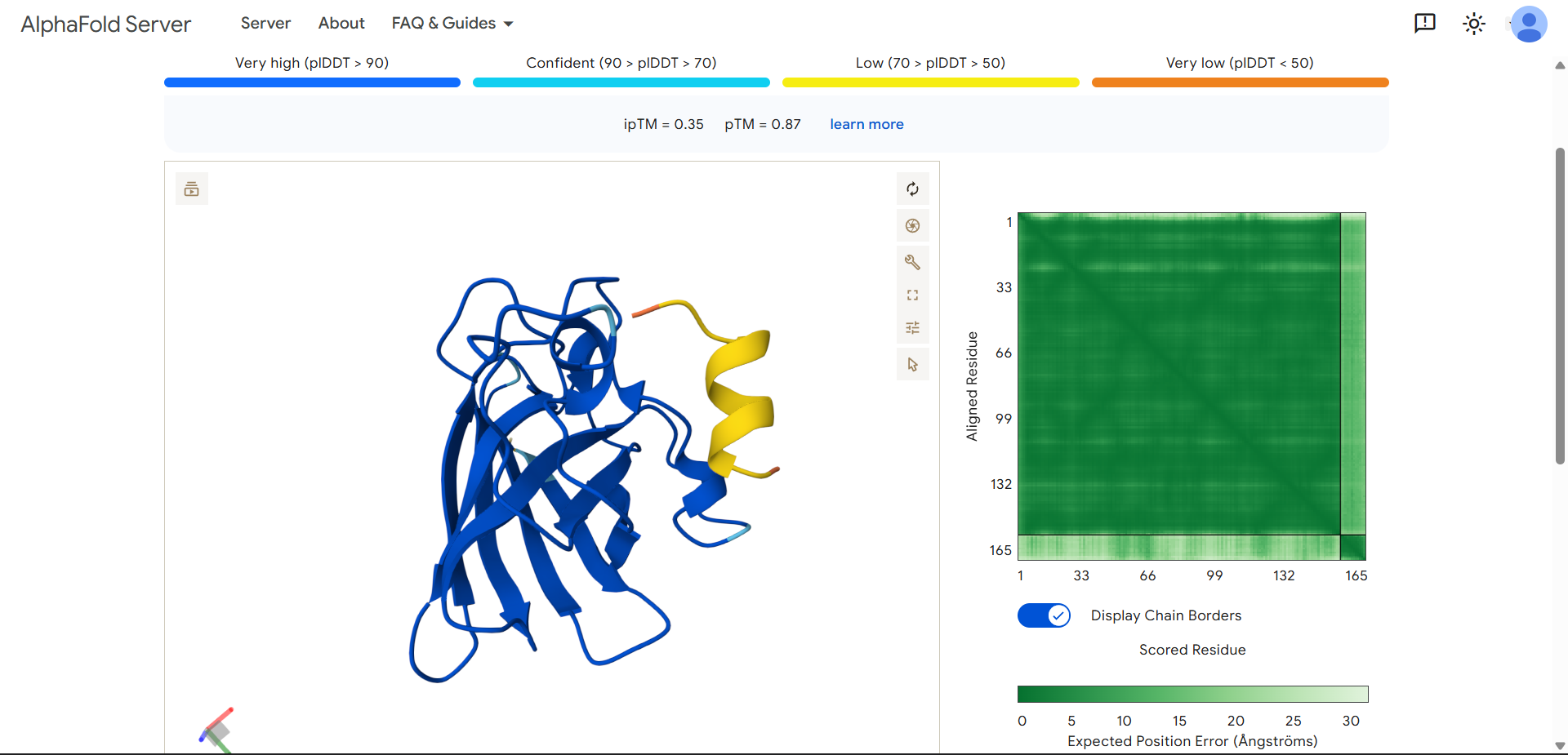
In recitation, we discussed that you will pick a protein for your homework that you find interesting. Which protein have you chosen and why? Using one of the tools described in recitation (NCBI, UniProt, google), obtain the protein sequence for the protein you chose.
[Example from our group homework, you may notice the particular format — The example below came from UniProt]
(95 amino acids; cysteine-rich protein with multiple disulfide bonds)
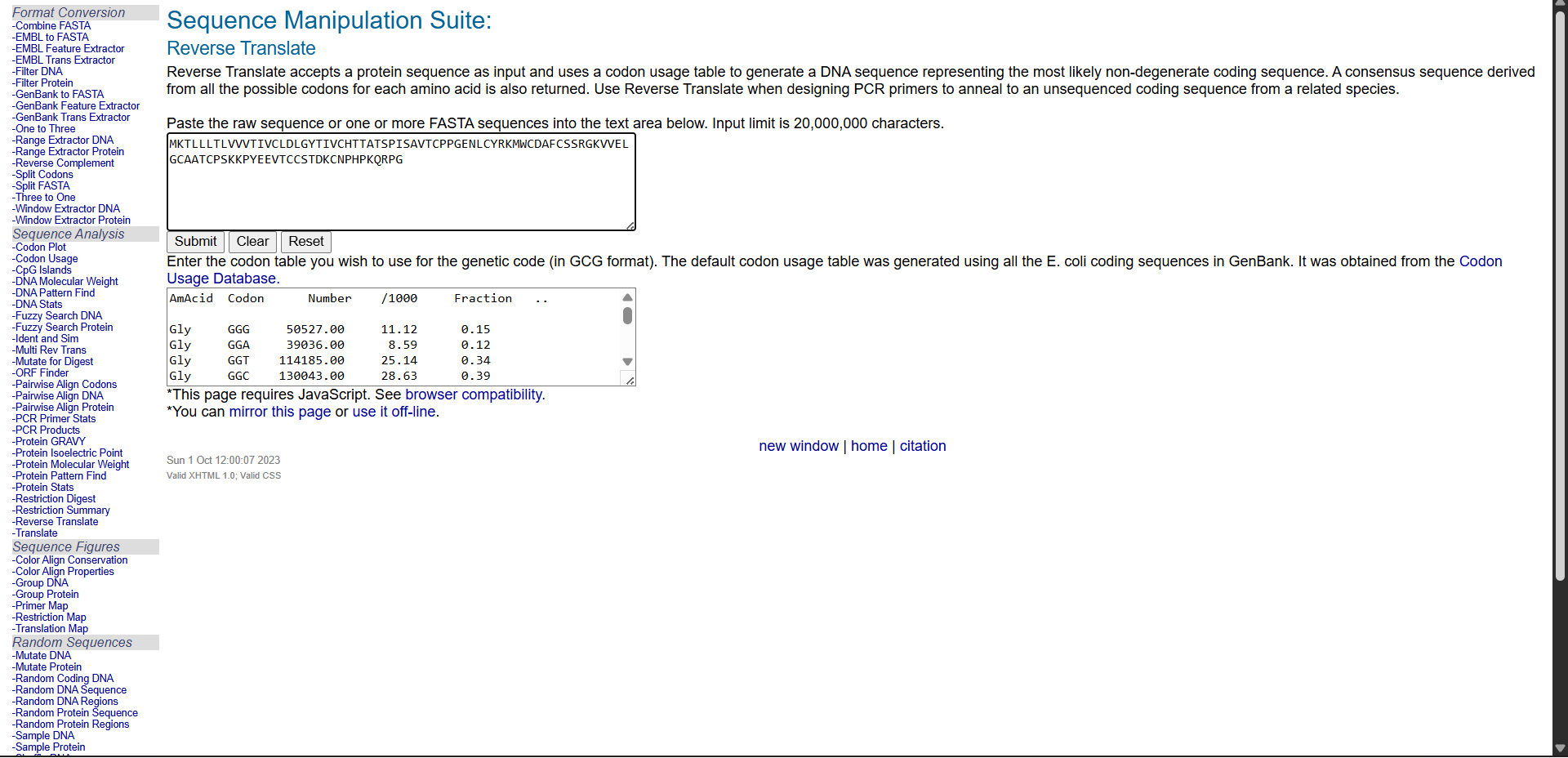
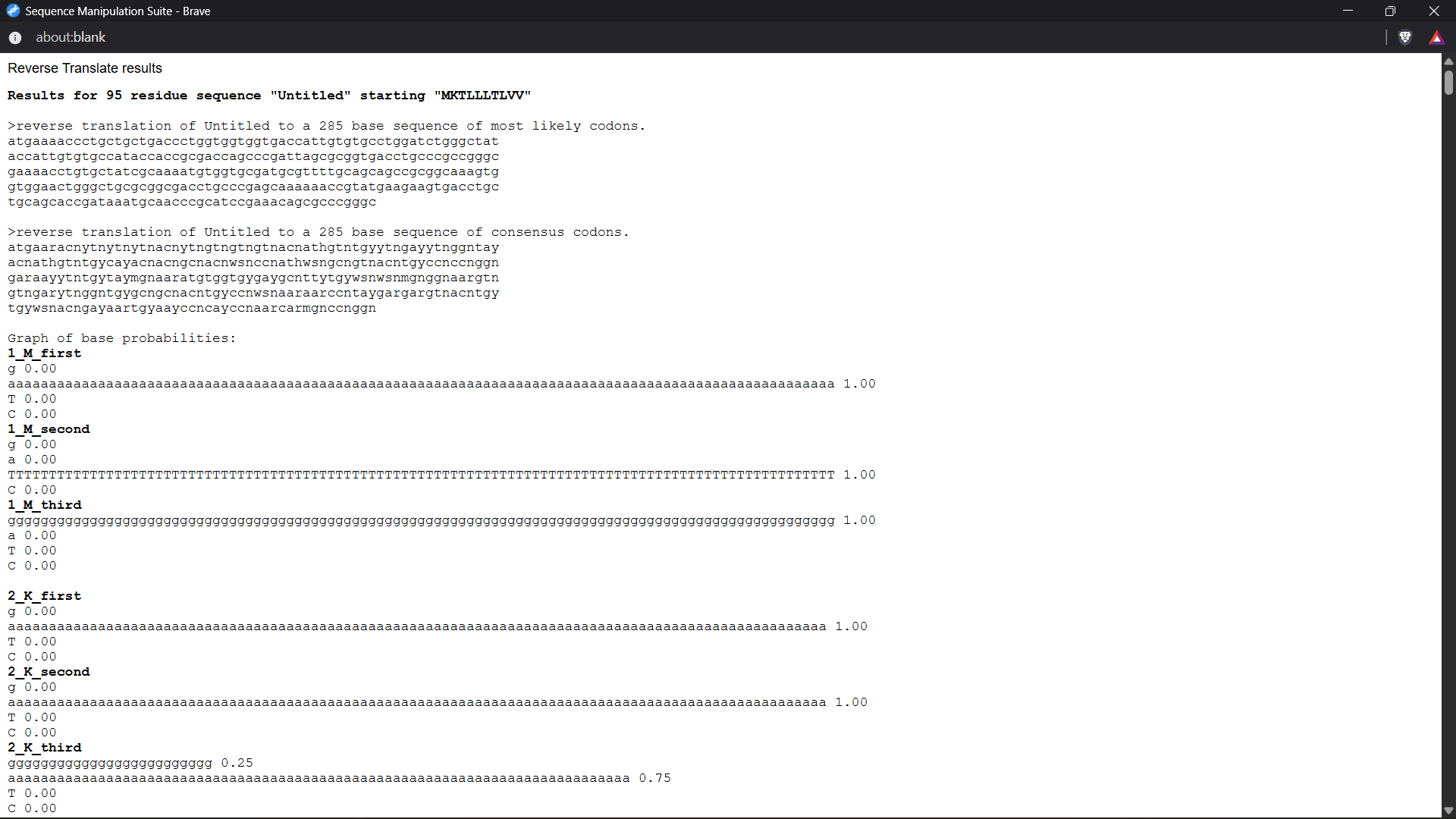
3.2. Reverse Translate: Protein (amino acid) sequence to DNA (nucleotide) sequence.
The Central Dogma discussed in class and recitation describes the process in which DNA sequence becomes transcribed and translated into protein. The Central Dogma gives us the framework to work backwards from a given protein sequence and infer the DNA sequence that the protein is derived from. Using one of the tools discussed in class, NCBI or online tools (google “reverse translation tools”), determine the nucleotide sequence that corresponds to the protein sequence you chose above.
Lysis protein DNA sequence atggaaacccgattccctcagcaatcgcagcaaactccggcatctactaatagacgccggccattcaaacatgaggattacccatgtcgaagacaacaaagaagttcaactctttatgtattgatcttcctcgcgatctttctctcgaaatttaccaatcaattgcttctgtcgctactggaagcggtgatccgcacagtgacgactttacagcaattgcttacttaa
As discussed in class, due to the degeneracy of the genetic code, multiple codons can encode the same amino acid. Therefore, reverse translation from a protein sequence to a DNA sequence is not unique.
Reverse translation was performed using the Bioinformatics reverse translation tool. Due to codon degeneracy, the resulting DNA sequence represents one possible coding sequence corresponding to the selected protein.
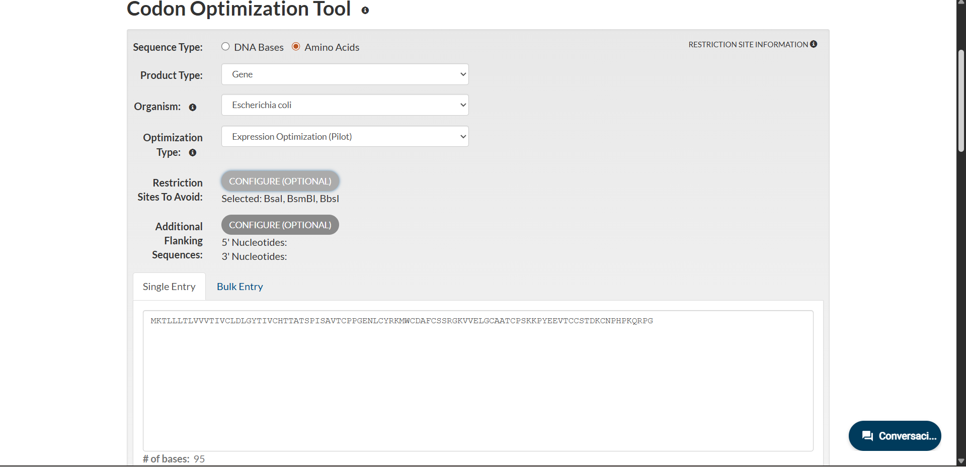
Once a nucleotide sequence of your protein is determined, you need to codon optimize your sequence. You may, once again, utilize google for a “codon optimization tool”. In your own words, describe why you need to optimize codon usage. Which organism have you chosen to optimize the codon sequence for and why?
Lysis protein DNA sequence with Codon-Optimization ATGGAAACCCGCTTTCCGCAGCAGAGCCAGCAGACCCCGGCGAGCACCAACCGCCGCCGCCCGTTCAAACATGAAGATTATCCGTGCCGTCGTCAGCAGCGCAGCAGCACCCTGTATGTGCTGATTTTTCTGGCGATTTTTCTGAGCAAATTCACCAACCAGCTGCTGCTGAGCCTGCTGGAAGCGGTGATTCGCACAGTGACGACCCTGCAGCAGCTGCTGACCTAA
Why is codon optimization necessary?
Although the genetic code is degenerate, meaning that multiple codons can encode the same amino acid, organisms do not use synonymous codons with equal frequency. Each organism has a preferred codon usage bias that reflects the abundance of its tRNAs.
If a gene containing rare codons is introduced into a heterologous host organism, several issues may arise:
Reduced translation efficiency
Lower protein yield
Increased risk of ribosome stalling
Potential misfolding due to slowed or irregular translation kinetics
Therefore, codon optimization is performed to adapt the coding sequence to the codon usage preferences of the chosen host organism, improving translation efficiency and overall protein production.
Selected organism for optimization
The coding sequence was optimized for expression in: Escherichia coli
Why E. coli?
It is the most widely used bacterial expression system.
It is cost-effective, fast-growing, and easy to genetically manipulate.
It is ideal for recombinant protein production.
Although α-bungarotoxin is a cysteine-rich protein containing multiple disulfide bonds, specialized strains (e.g., oxidative cytoplasm strains) or periplasmic targeting strategies can facilitate proper folding.
Codon-optimized sequence for E. coli
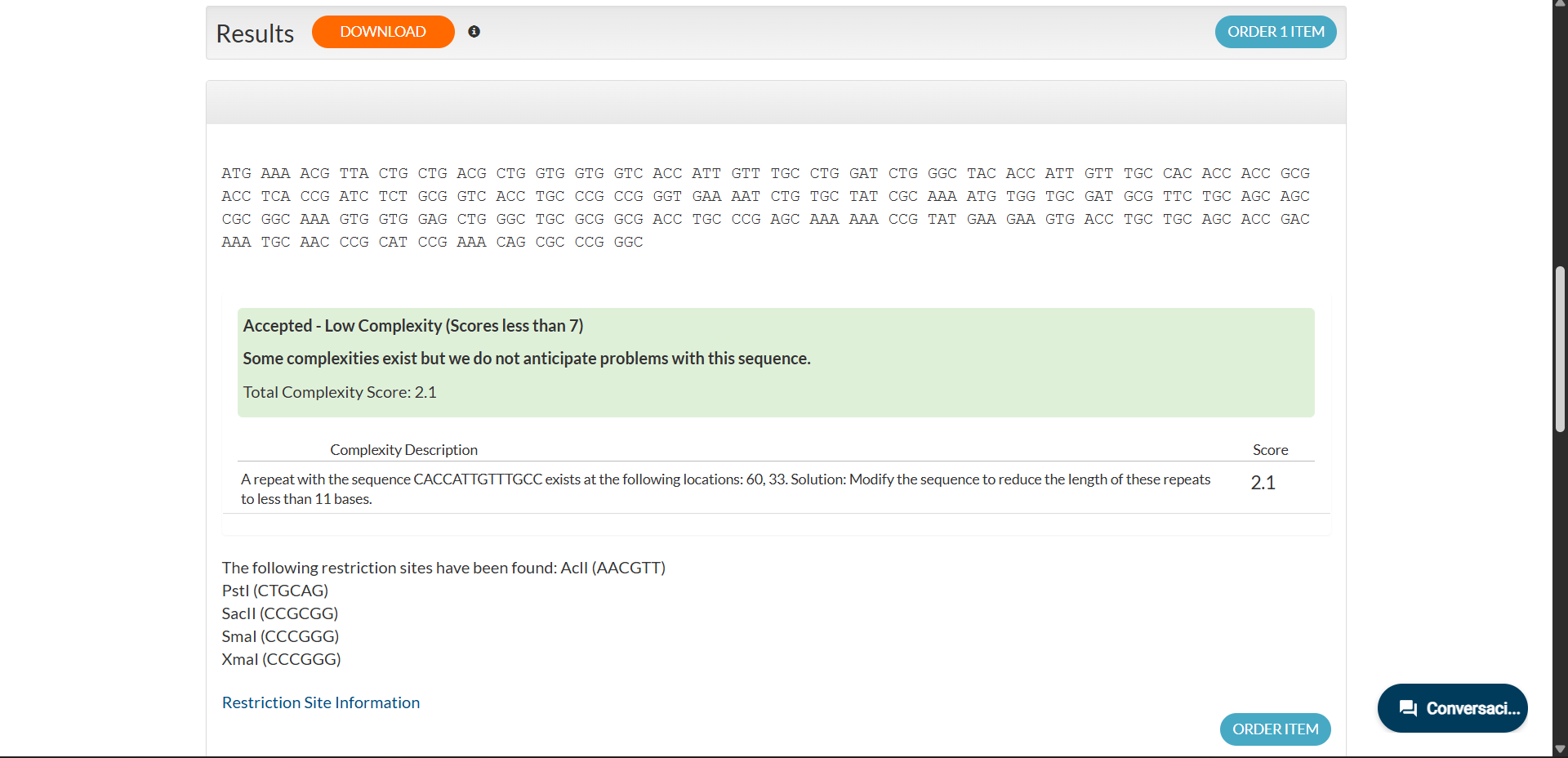
Codon optimization was performed using the Expression Optimization (Pilot) algorithm provided by Integrated DNA Technologies. The amino acid sequence was optimized for expression in Escherichia coli while avoiding BsaI, BsmBI and BbsI restriction sites.
The resulting optimized coding sequence (285 bp) is:
Sequence analysis indicated low complexity (score 2.1), suggesting no anticipated synthesis issues. Internal restriction sites unrelated to the cloning strategy were detected but do not interfere with the intended design.
3.4. We have a sequence! Now what?
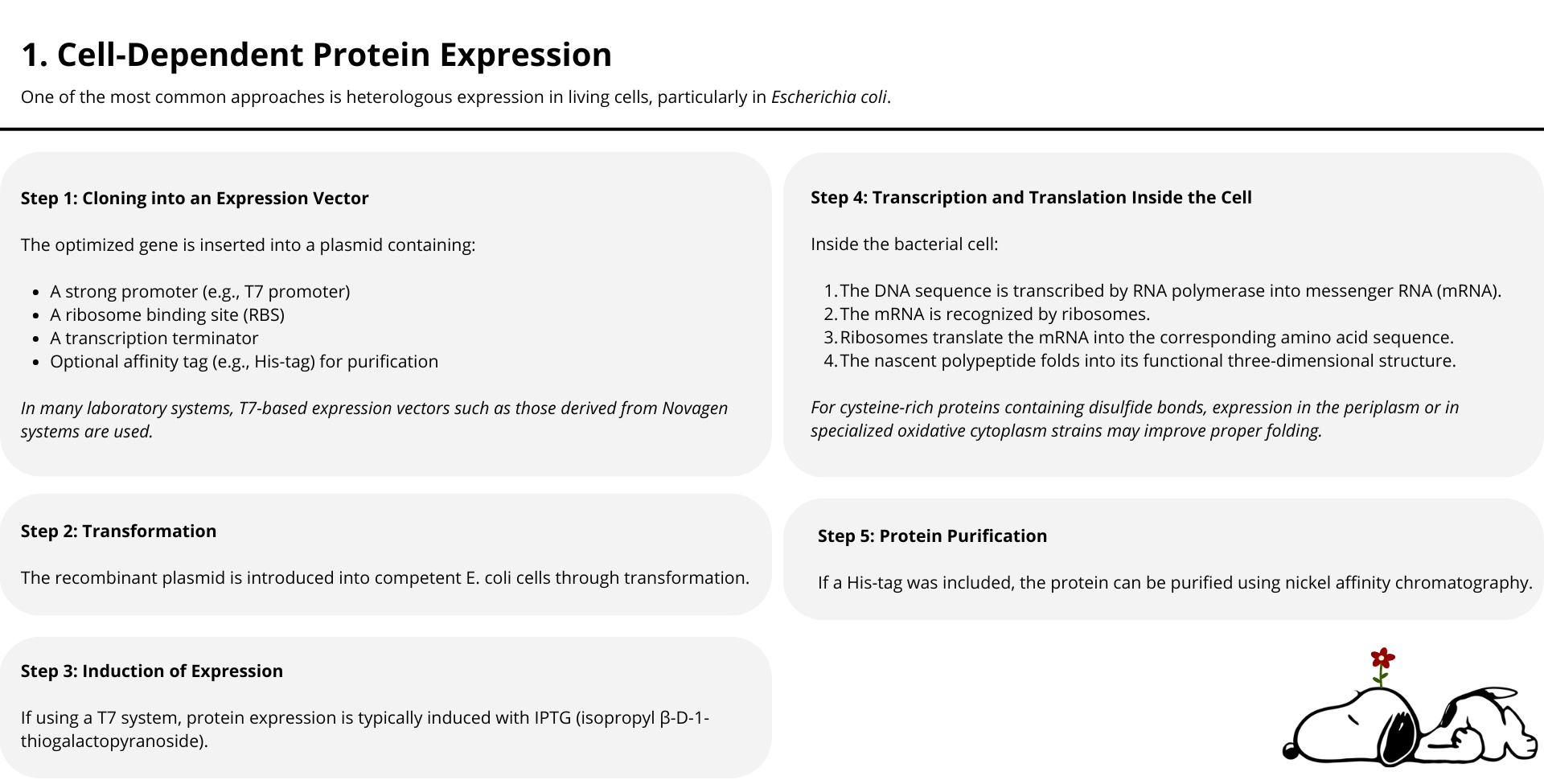
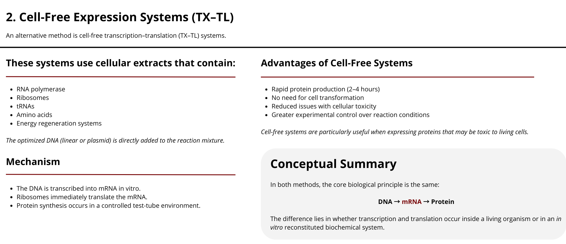
What technologies could be used to produce this protein from your DNA? Describe in your words the DNA sequence can be transcribed and translated into your protein. You may describe either cell-dependent or cell-free methods, or both.
Once the codon-optimized DNA sequence has been obtained, several biotechnological strategies can be used to produce the corresponding protein. These methods rely on the fundamental biological processes of transcription and translation. Protein production can be achieved using either cell-dependent systems or cell-free expression systems.
3.5. [Optional] How does it work in nature/biological systems?
Describe how a single gene codes for multiple proteins at the transcriptional level.
Try aligning the DNA sequence, the transcribed RNA, and also the resulting translated Protein!!! See example below.
In natural biological systems, a single gene can give rise to multiple protein products. Although the classical view suggests that one gene encodes one protein, several regulatory mechanisms allow diversification at the transcriptional and post-transcriptional levels.
Mechanisms that allow one gene to produce multiple proteins
1. Alternative splicing
In eukaryotic organisms, genes contain exons and introns. During RNA processing, introns are removed and exons are joined together. However, different combinations of exons can be assembled, producing distinct mRNA variants from the same gene.
This process, known as alternative splicing, results in different protein isoforms with potentially different functions.
2. Alternative promoters
A single gene may contain multiple promoter regions. Depending on which promoter is activated, transcription may begin at different start sites, generating mRNAs with different 5′ ends. This can influence translation efficiency or alter the protein sequence.
3. Alternative translation initiation sites
Some mRNAs contain more than one possible start codon (AUG). Ribosomes may initiate translation at different positions, leading to proteins of different lengths.
4. RNA editing
In certain organisms, specific nucleotides in the RNA sequence are chemically modified after transcription. This can change codons and therefore alter the amino acid sequence of the final protein.
Alignment example: DNA → RNA → Protein
Using our optimized coding sequence as an example:
DNA (coding strand)
5′- ATG AAA ACG TTA CTG CTG -3′
Transcribed mRNA
(Thymine is replaced by uracil)
5′- AUG AAA ACG UUA CUG CUG -3′
Translated protein
Met – Lys – Thr – Leu – Leu – Leu
This alignment illustrates the central dogma of molecular biology:
DNA → RNA → Protein
In prokaryotes such as Escherichia coli, transcription and translation are coupled and occur simultaneously in the cytoplasm. In contrast, in eukaryotic cells, transcription occurs in the nucleus and translation occurs in the cytoplasm after RNA processing.
Part 4: Preparing a Twist DNA Synthesis Order
Assignees for the following sections
MIT/Harvard students
Required
Committed Listeners
Required
SECTION A. BENCHLING
This is a practice exercise, not necessarily the real Twist order!
We’ll make a sequence that will allow E. coli to glow fluorescent green under UV light by constitutively (always) expressing sfGFP (a green fluorescent protein):
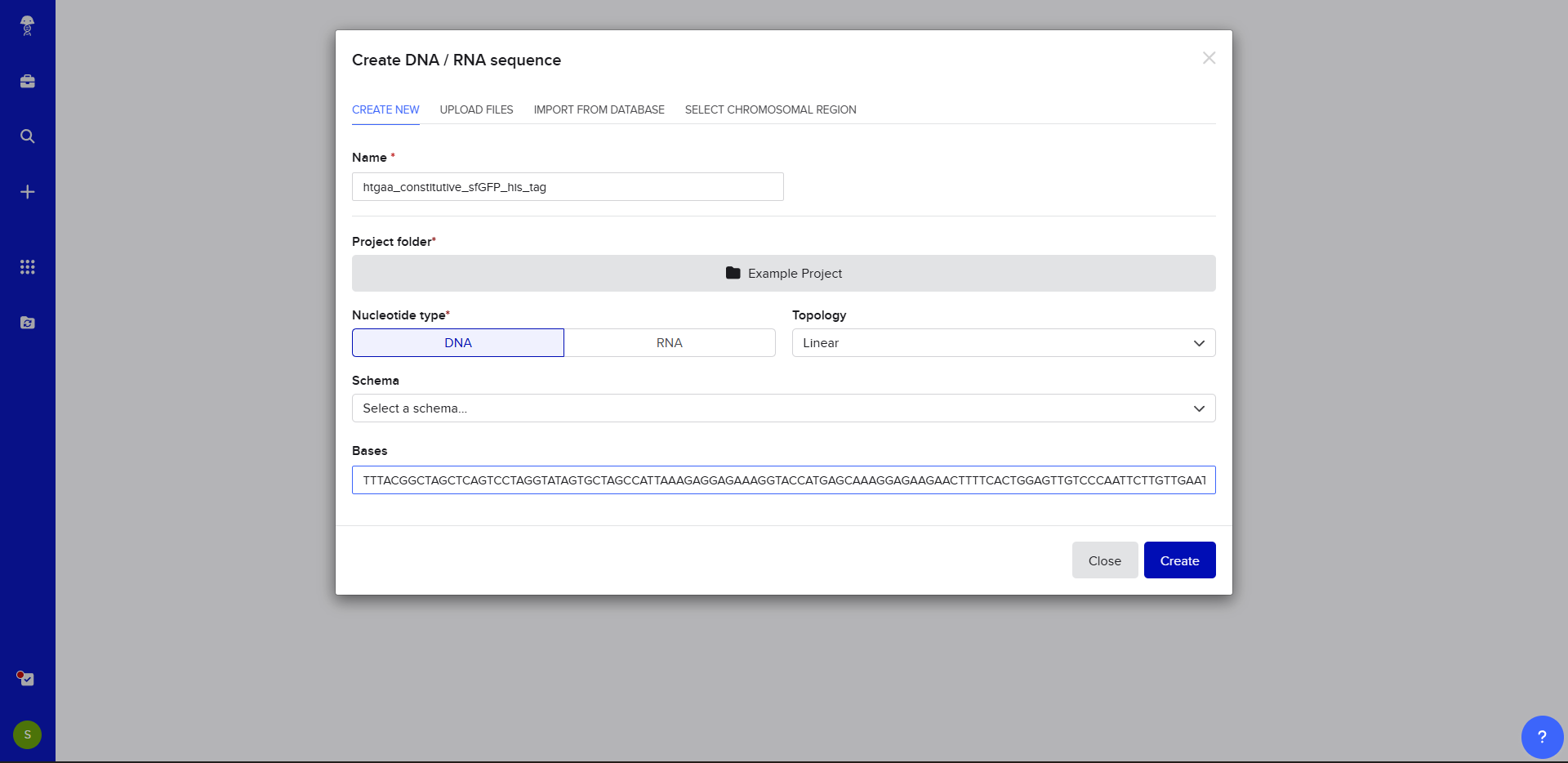
In Benchling, we select New DNA/RNA sequence
Now name the insert sequence and select DNA with a Linear topology (this is a linear sequence that will be inserted into a circular backbone vector of our choosing).
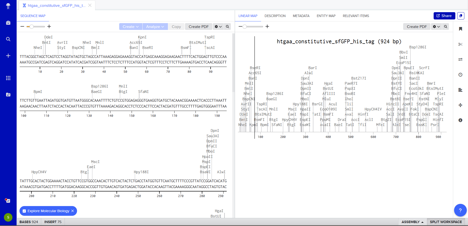
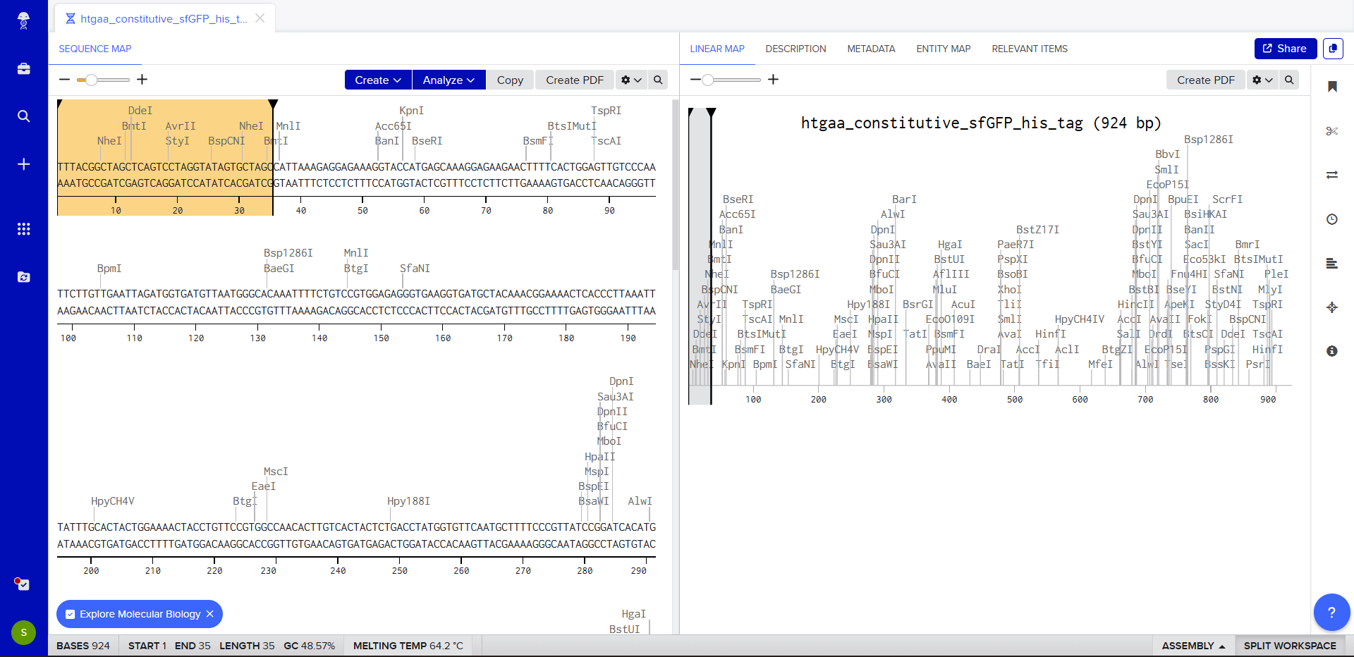
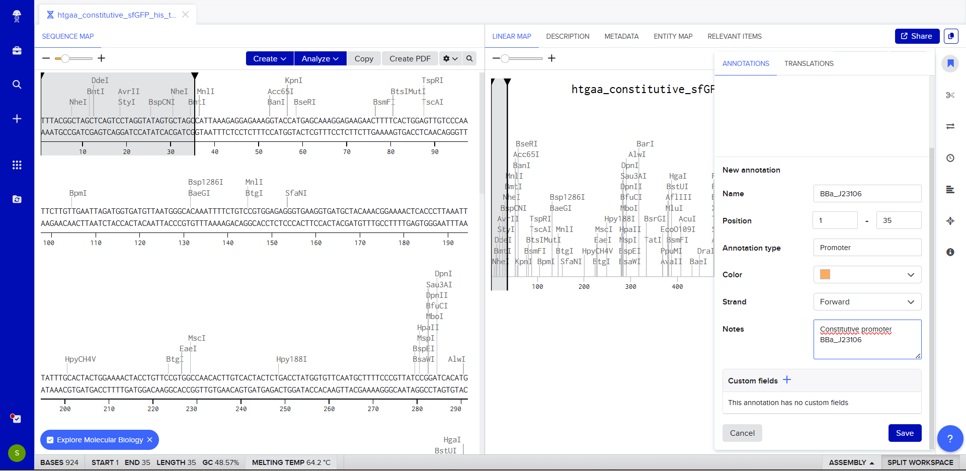
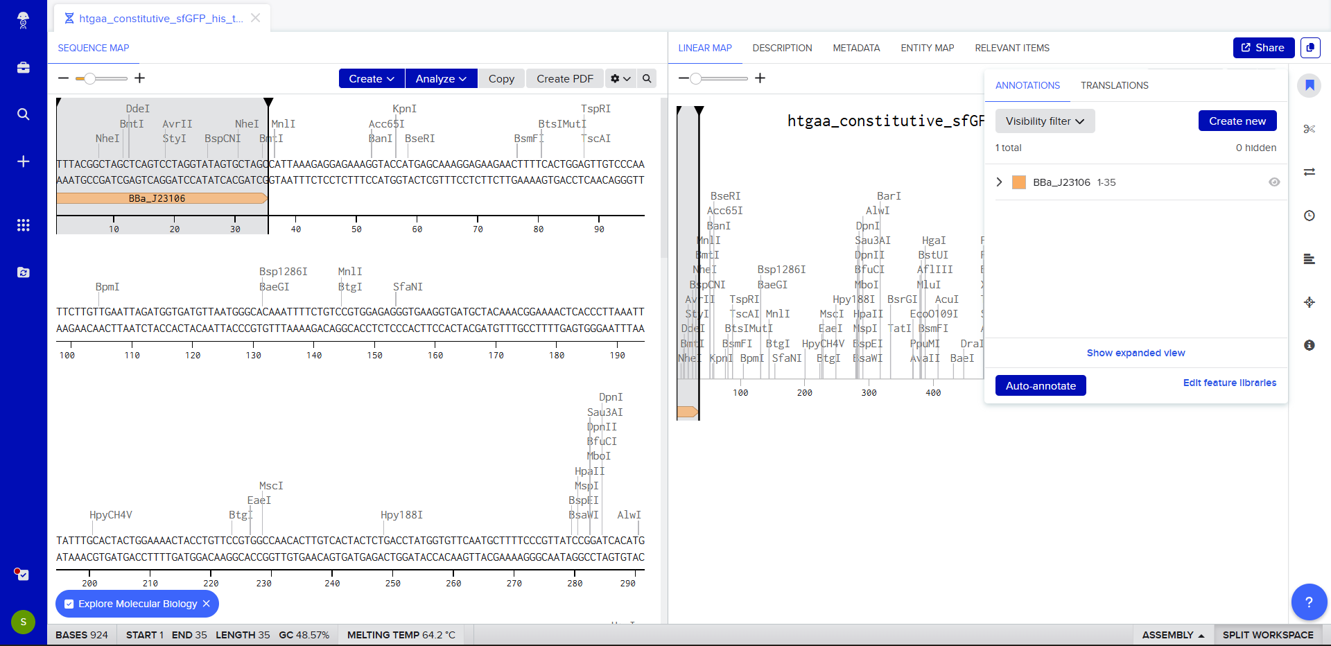
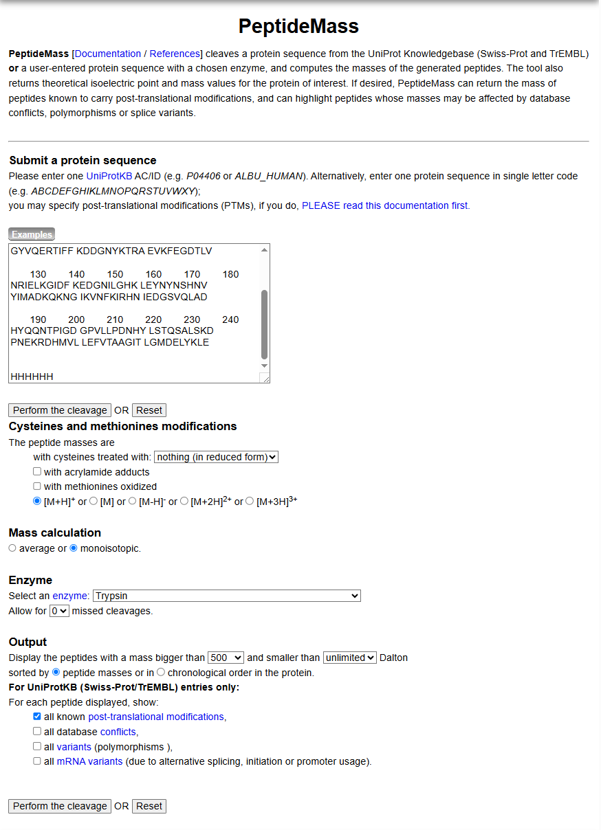
We go through each piece of the given DNA sequences highlighted below (Promoter, RBS, Start Codon, Coding Sequence, His Tag, Stop Codon, Terminator) and paste the sequences into the Benchling file one after the other (replacing the coding sequence with the codon optimized DNA sequence of interest). Each time we add a new piece of the sequence, we make sure to annotate by right clicking over the sequence and creating an annotation that describes what each piece (e.g., Promoter, RBS, etc.) is (see image below).
RBS (e.g. BBa_B0034 with spacers for optimal expression) CATTAAAGAGGAGAAAGGTACC
Start Codon ATG
Coding Sequence (your codon optimized DNA for a protein of interest, sfGFP for example) AGCAAAGGAGAAGAACTTTTCACTGGAGTTGTCCCAATTCTTGTTGAATTAGATGGTGATGTTAATGGGCACAAATTTTCTGTCCGTGGAGAGGGTGAAGGTGATGCTACAAACGGAAAACTCACCCTTAAATTTATTTGCACTACTGGAAAACTACCTGTTCCGTGGCCAACACTTGTCACTACTCTGACCTATGGTGTTCAATGCTTTTCCCGTTATCCGGATCACATGAAACGGCATGACTTTTTCAAGAGTGCCATGCCCGAAGGTTATGTACAGGAACGCACTATATCTTTCAAAGATGACGGGACCTACAAGACGCGTGCTGAAGTCAAGTTTGAAGGTGATACCCTTGTTAATCGTATCGAGTTAAAGGGTATTGATTTTAAAGAAGATGGAAACATTCTTGGACACAAACTCGAGTACAACTTTAACTCACACAATGTATACATCACGGCAGACAAACAAAAGAATGGAATCAAAGCTAACTTCAAAATTCGCCACAACGTTGAAGATGGTTCCGTTCAACTAGCAGACCATTATCAACAAAATACTCCAATTGGCGATGGCCCTGTCCTTTTACCAGACAACCATTACCTGTCGACACAATCTGTCCTTTCGAAAGATCCCAACGAAAAGCGTGACCACATGGTCCTTCTTGAGTTTGTAACTGCTGCTGGGATTACACATGGCATGGATGAGCTCTACAAA
7x His Tag (Let’s add a 7×His tag at the C-terminus of the protein to enable protein purification from E. coli) CATCACCATCACCATCATCAC
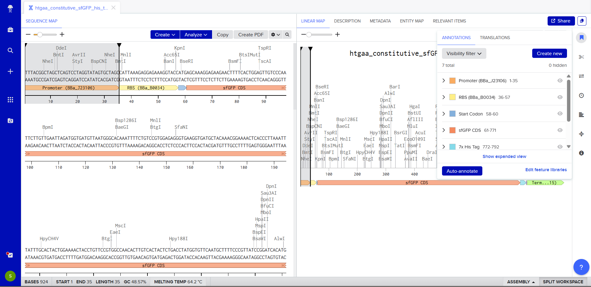
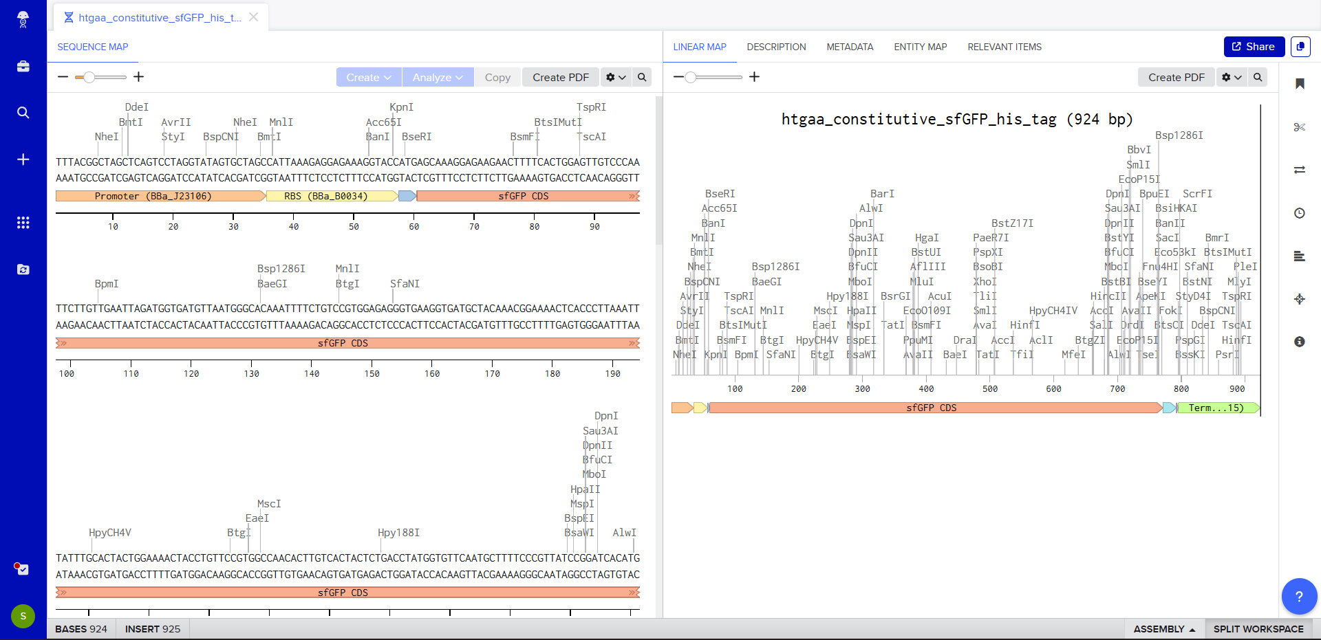
Once this is completed, we click on Linear Map to preview the entire sequence.
Note: This is not required for this exercise, but to share the design with others, ensure that link sharing is turned on!
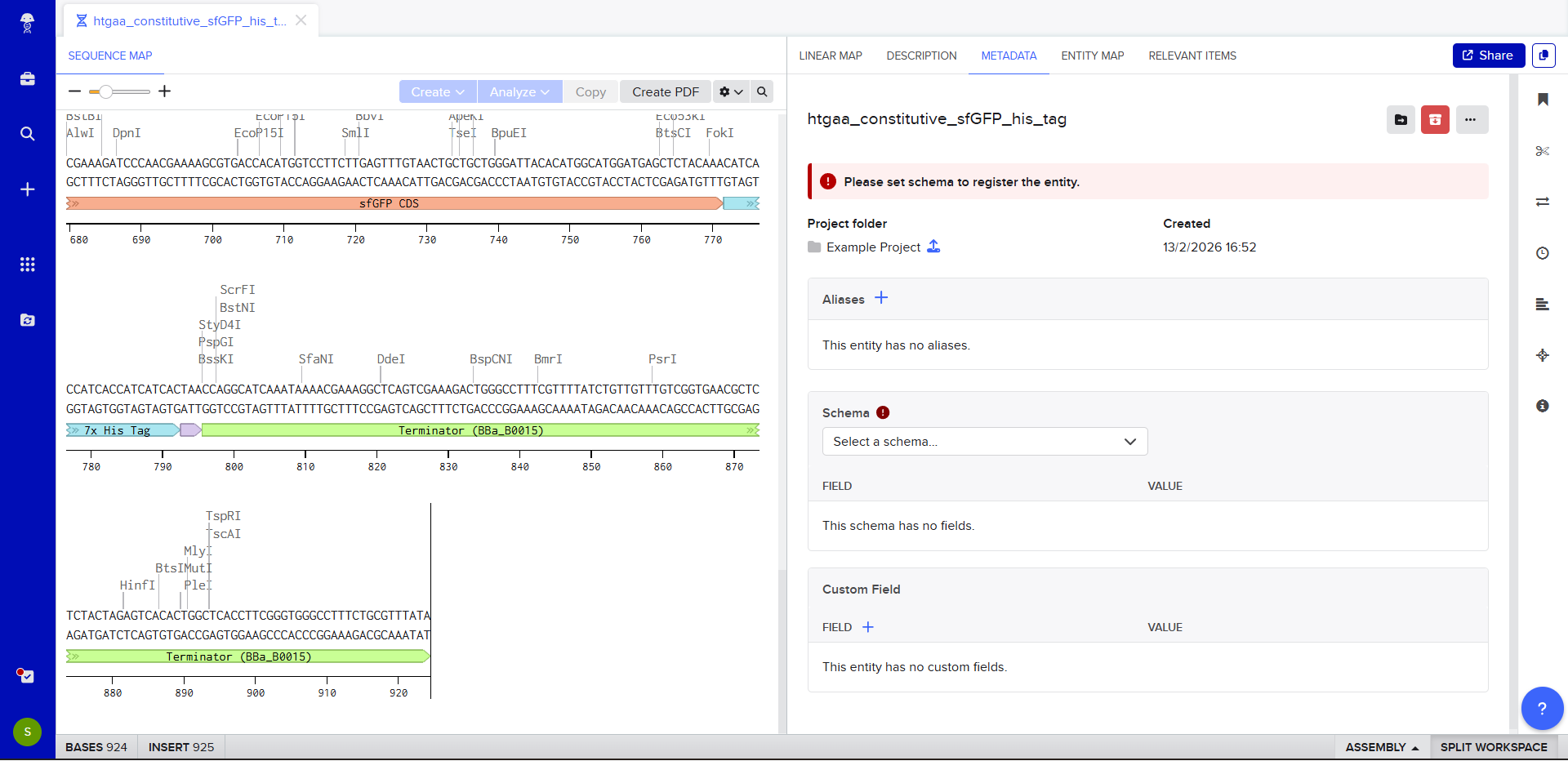
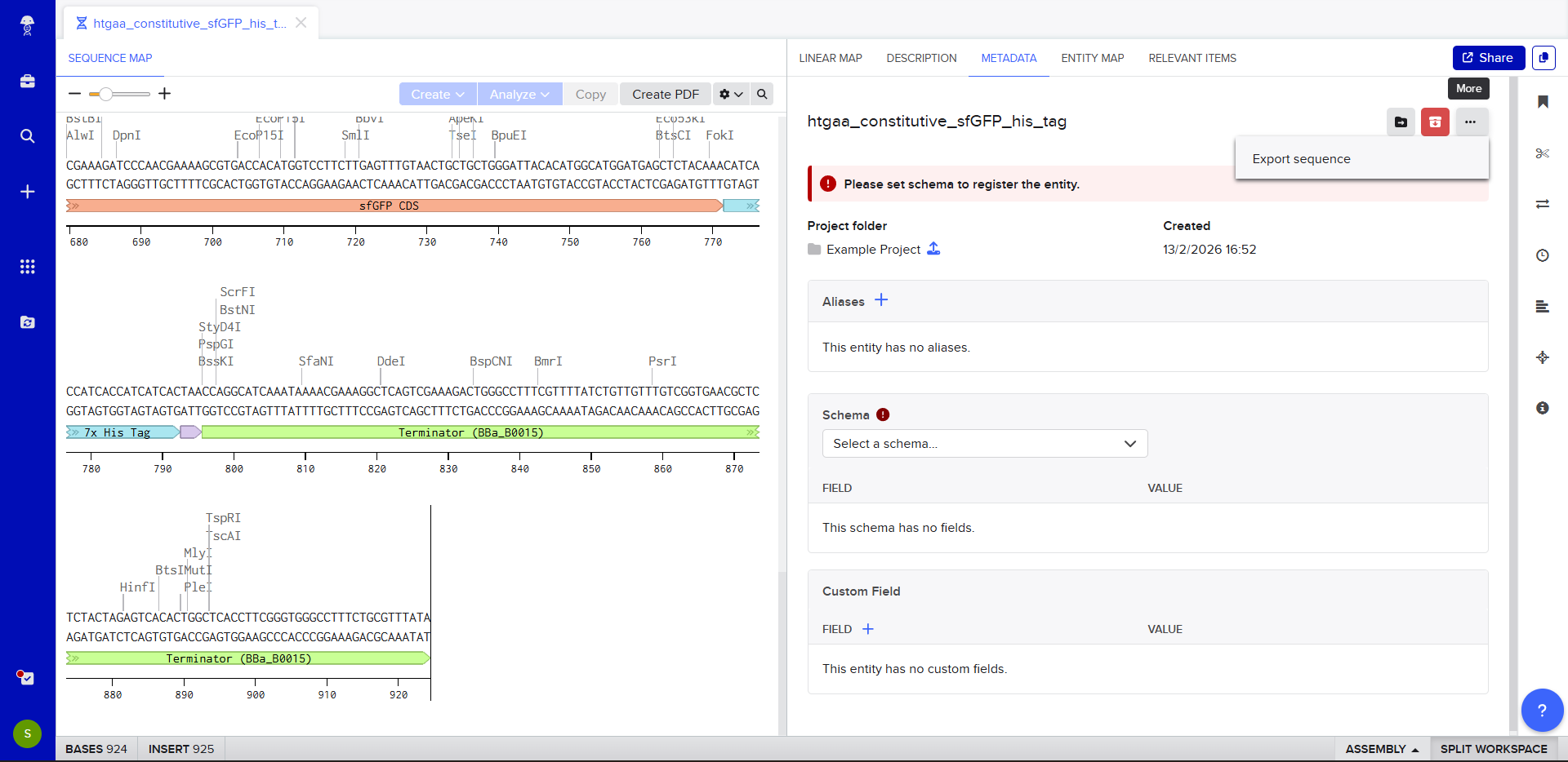
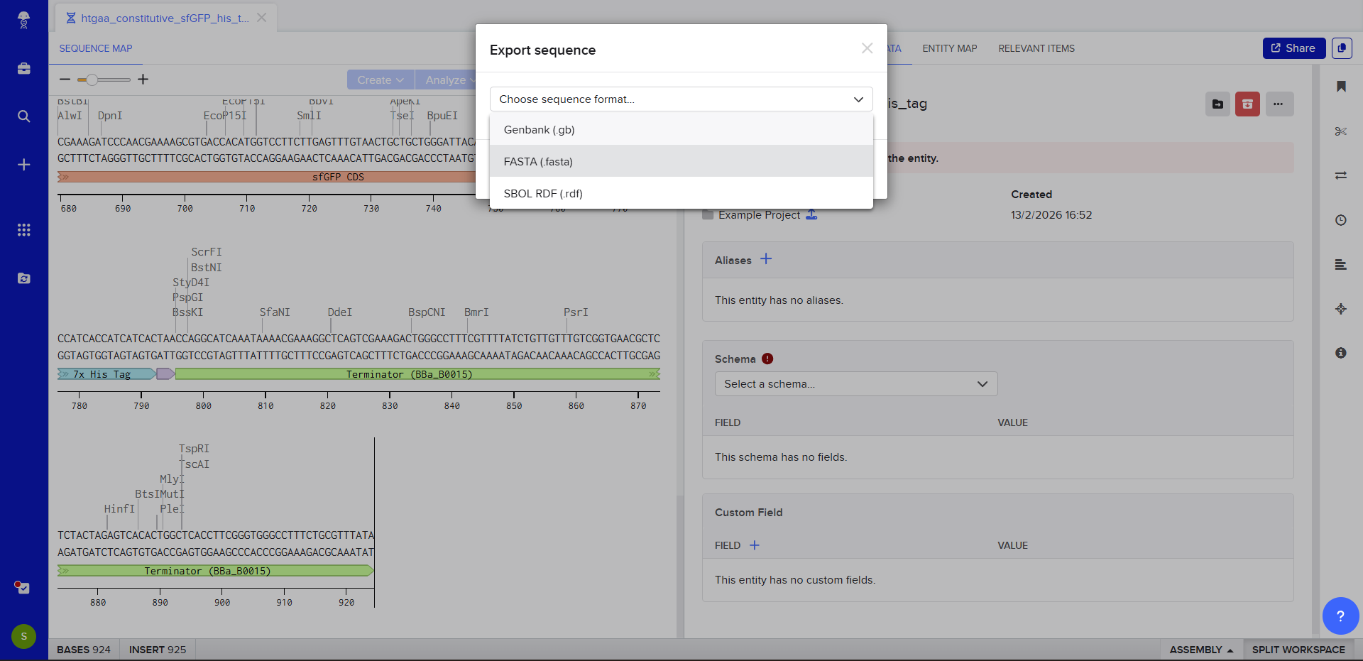
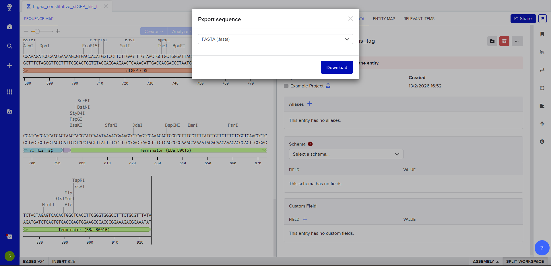
The insert sequence that was built is commonly referred to as an expression cassette in molecular biology (a sequence you can drop into any vector and it’ll perform its function). We now download the FASTA file for the sequence made.
It’s helpful to visualize DNA designs using SBOL Canvas (Synthetic Biology Open Language) to convey the design. Here’s an example of what we just annotated in Benchling:
SECTION B. TWIST
Part 5: DNA Read/Write/Edit
Assignees for the following sections
MIT/Harvard students
Required
Committed Listeners
Required
5.1 DNA Read
(i) What DNA would you want to sequence (e.g., read) and why? This could be DNA related to human health (e.g. genes related to disease research), environmental monitoring (e.g., sewage waste water, biodiversity analysis), and beyond (e.g. DNA data storage, biobank).
For my project — Reversible Cell-Free Biosensor for ROS-Mediated Radiation Damage — we would want to sequence three categories of DNA:
1. The ROS-responsive promoter region
- Specifically, oxidative stress–responsive regulatory elements (e.g., OxyR/SoxR-regulated promoters from E. coli).
Why?
- To verify the exact sequence integrity of the promoter controlling our reporter.
- Small mutations in regulatory regions can drastically alter activation threshold, leakiness, or response dynamics.
- Since our system depends on reversible, tunable activation (not binary irreversible switching), promoter fidelity is critical for predictable behavior.
2. The full genetic construct used in the TX–TL system
This includes:
- Promoter
- RBS
- Reporter gene (e.g., GFP variant)
- Degron tag
- Terminator
Why?
- To confirm assembly correctness after cloning or synthesis.
- To ensure no frameshifts, truncations, or rearrangements occurred.
- To validate that the degron sequence is intact (since reversibility depends on controlled protein degradation).
3. DNA stability after ROS exposure (damage assessment)
- Because the biosensor operates in oxidative environments, we may also sequence recovered plasmid DNA after repeated ROS cycles.
Why?
- To assess oxidative damage accumulation.
- To evaluate mutation rates under stress.
- To determine long-term reusability limits of the system.
This directly connects to governance and safety: understanding failure modes prevents misleading signal interpretation.
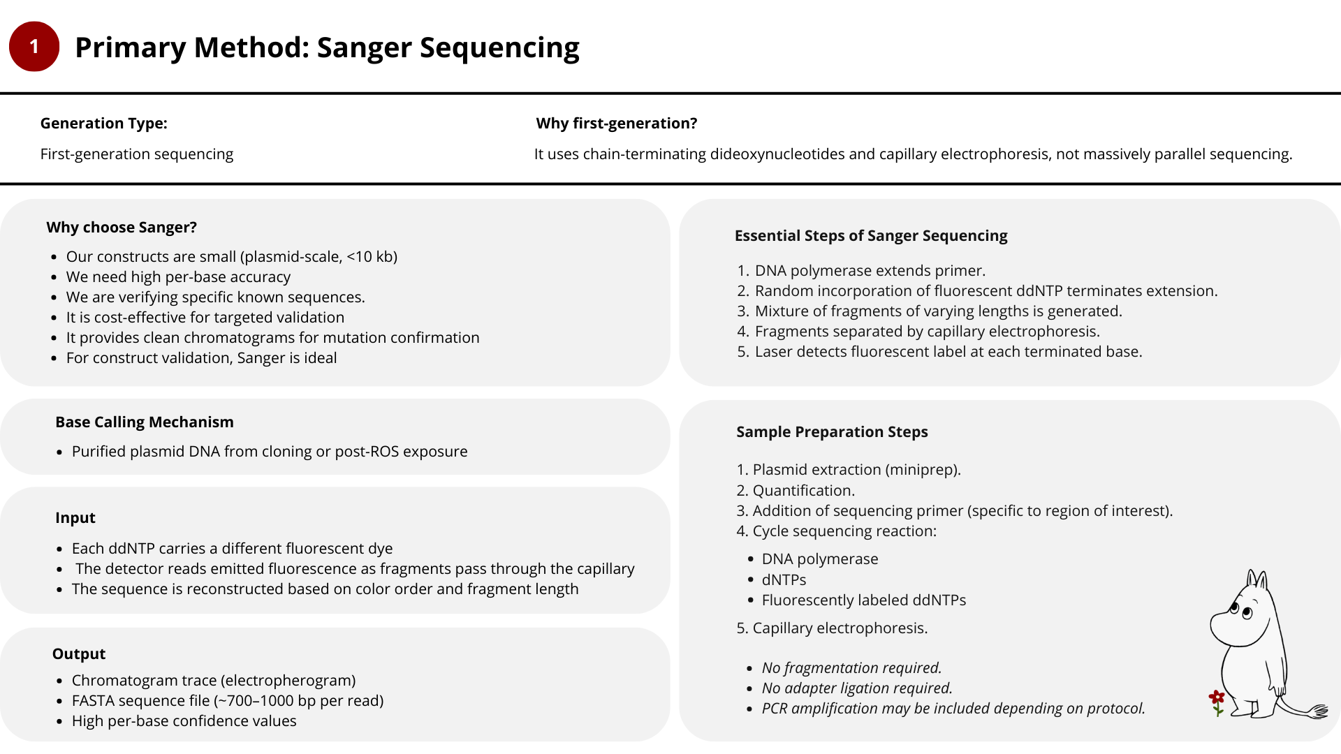
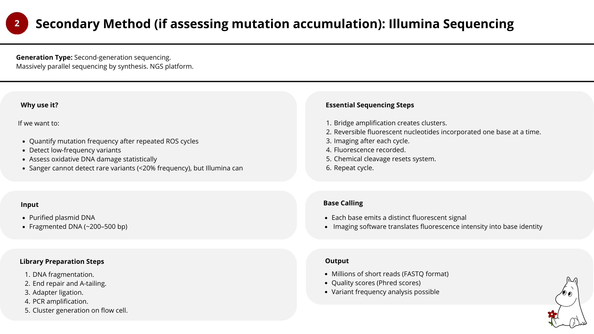
(ii) In lecture, a variety of sequencing technologies were mentioned. What technology or technologies would you use to perform sequencing on your DNA and why?
Also answer the following questions:
Is your method first-, second- or third-generation or other? How so?
What is your input? How do you prepare your input (e.g. fragmentation, adapter ligation, PCR)? List the essential steps.
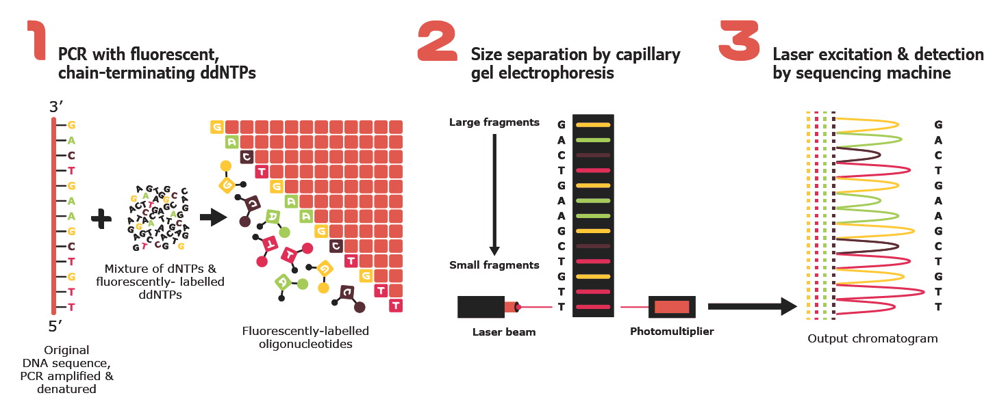
What are the essential steps of your chosen sequencing technology, how does it decode the bases of your DNA sample (base calling)?
What is the output of your chosen sequencing technology?
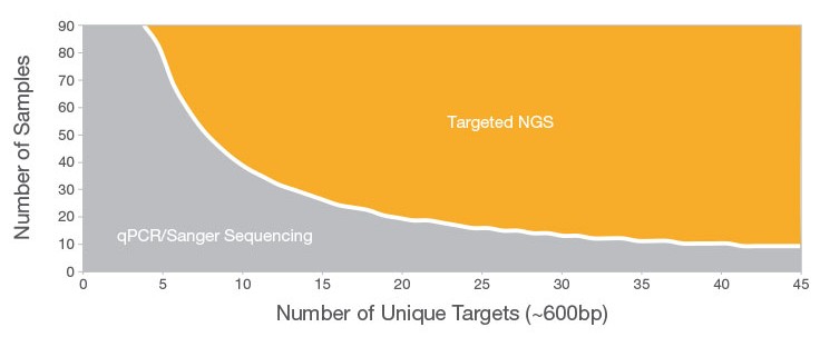
For this project, I would use a combination of Sanger sequencing and Illumina sequencing, depending on the question being asked.
Sanger sequencing is sufficient and ideal for construct validation.
Illumina sequencing becomes valuable when studying oxidative mutation accumulation and long-term robustness.
This sequencing strategy directly supports:
Reliability
Reversibility characterization
Governance considerations
Failure-mode understanding
Safe system deployment
5.2 DNA Write
(i) What DNA would you want to synthesize (e.g., write) and why? These could be individual genes, clusters of genes or genetic circuits, whole genomes, and beyond. As described in class thus far, applications could range from therapeutics and drug discovery (e.g., mRNA vaccines and therapies) to novel biomaterials (e.g. structural proteins), to sensors (e.g., genetic circuits for sensing and responding to inflammation, environmental stimuli, etc.), to art (DNA origamis). If possible, include the specific genetic sequence(s) of what you would like to synthesize! You will have the opportunity to actually have Twist synthesize these DNA constructs! :)
For the reversible ROS-mediated hydrogel biosensor, we would synthesize a minimal genetic circuit designed for oxidative stress detection and transient fluorescent output.
The construct would include:
A ROS-responsive promoter (e.g., OxyR-regulated promoter)
A ribosome binding site (RBS)
A fluorescent reporter gene (e.g., sfGFP)
A short degron tag to ensure rapid protein degradation
A transcriptional terminator
Why synthesize this DNA?
Because:
The promoter must be precisely tuned to oxidative stress.
The degron must be fused correctly to ensure reversibility.
The full construct must function in a cell-free TX–TL system.
Synthetic DNA reduces cloning errors.
It enables modular optimization.
We are not synthesizing a whole genome. We are synthesizing a minimal functional sensing circuit embedded in a biomaterial.
(ii) What technology or technologies would you use to perform this DNA synthesis and why?
Also answer the following questions:
What are the essential steps of your chosen sequencing methods?
What are the limitations of your sequencing method (if any) in terms of speed, accuracy, scalability?
We would use commercial gene synthesis services, such as those provided by:
Twist Bioscience
These companies use high-throughput DNA synthesis platforms based on phosphoramidite chemistry and silicon-based parallel synthesis.
Simplified process:
Attach first base to solid surface.
Add chemically protected nucleotide.
Remove protective group.
Add next nucleotide.
Repeat cycle.
Each cycle adds ONE base. This is automated.
For longer fragments:
Short oligos are synthesized.
Then assembled enzymatically into longer genes.
Verified by sequencing.
5.3 DNA Edit
(i) What DNA would you want to edit and why? In class, George shared a variety of ways to edit the genes and genomes of humans and other organisms. Such DNA editing technologies have profound implications for human health, development, and even human longevity and human augmentation. DNA editing is also already commonly leveraged for flora and fauna, for example in nature conservation efforts, (animal/plant restoration, de-extinction), or in agriculture (e.g. plant breeding, nitrogen fixation). What kinds of edits might you want to make to DNA (e.g., human genomes and beyond) and why?
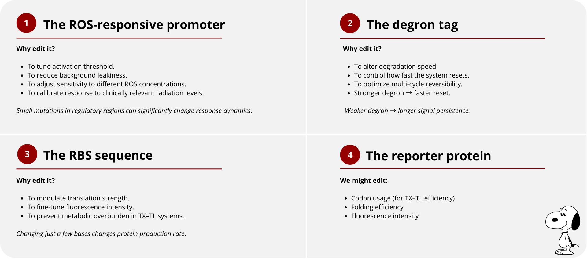
For this biosensor, I would edit the genetic circuit itself to optimize sensing dynamics, reversibility, and robustness.
Specifically, we would edit:
(ii) What technology or technologies would you use to perform these DNA edits and why?
Also answer the following questions:
How does your technology of choice edit DNA? What are the essential steps?
What preparation do you need to do (e.g. design steps) and what is the input (e.g. DNA template, enzymes, plasmids, primers, guides, cells) for the editing?
What are the limitations of your editing methods (if any) in terms of efficiency or precision?
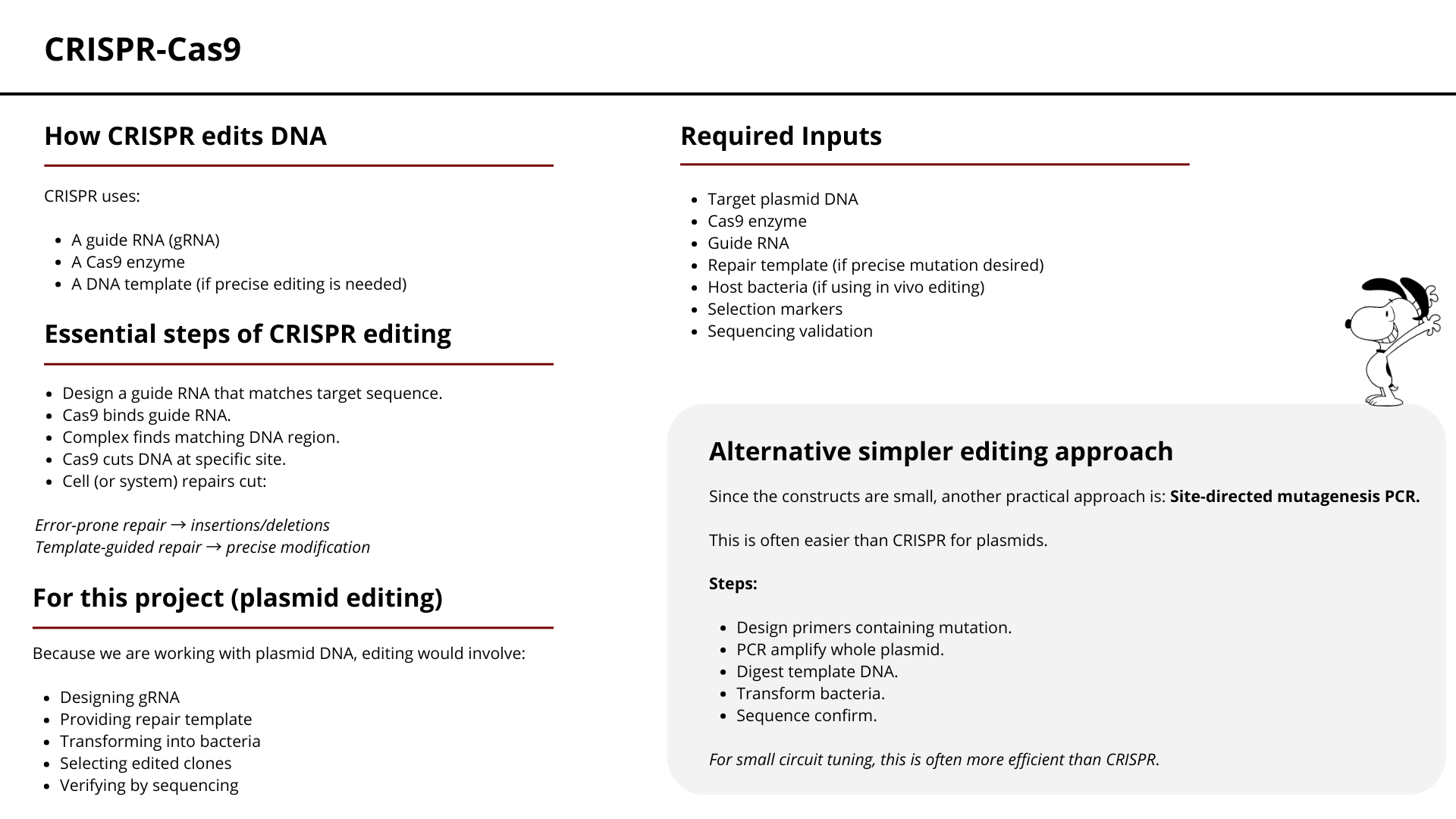
The most appropriate technology for precise edits in genetic constructs would be:
CRISPR-based editing systems.
Specifically: CRISPR-Cas9
Limitations of DNA Editing Methods
1. Off-target effects (CRISPR)
Cas9 can cut unintended regions.
Less relevant for small plasmids, more relevant for genomes.
2. Efficiency variability
Not all cells incorporate edits.
Requires screening.
3. Repair pathway dependence
Precise edits require homologous recombination.
Not always efficient.
4. Context sensitivity
Changing one base can unpredictably alter promoter behavior.
Requires iterative testing.
For this project DNA editing is not strictly required for initial system implementation. However, it would be essential for iterative optimization of promoter sensitivity, degradation kinetics, and response tuning.
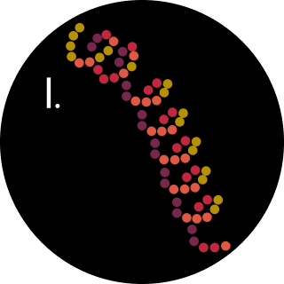
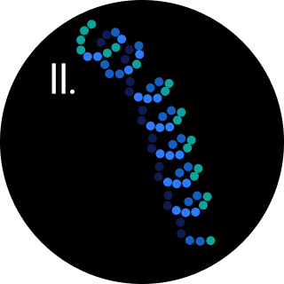
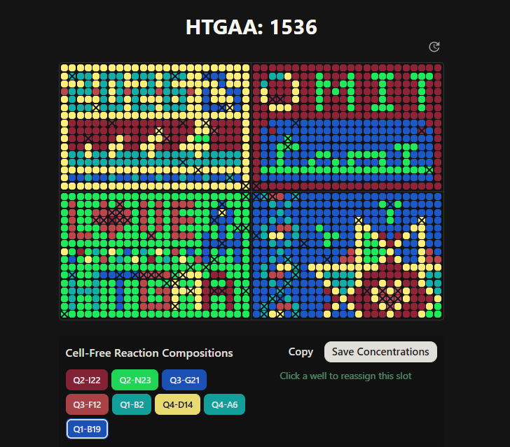
The original idea was to create a piece based on gothic arquitecture featuring a stained glass rose window
The inspo vs the reallity.
However, the results where closer to a Mario Bros castle and I didn’t quite like it, so instead, I made a second attempt with two different options; one for my gothic rose window greed and another one more simple with a Snoopy design, thinking more on the time recuired for it to be created on the Opentron machine.
The first idea vs the final idea
Rose window (left), full final design (center) and simplified final design (right).
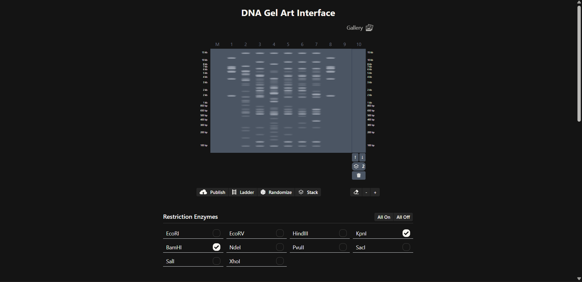
The link for the final published design on te GUI site is this: Click here
Using the coordinates from the GUI, follow the instructions in the HTGAA26 Opentrons Colab to write your own Python script which draws your design using the Opentrons.
You may use AI assistance for this coding — Google Gemini is integrated into Colab (see the stylized star bottom center); it will do a good job writing functional Python, while you probably need to take charge of the art concept.
If you’re a proficient programmer and you’d rather code something mathematical or algorithmic instead of using your GUI coordinates, you may do that instead.
For the Python code in Google Colab:
I did try to make the Python file aside from the Ronan’s site Python download and I encounter a few issues while coding.
HTGAA Opentrons Setup Code Analysis
1. Environment Setup
import sys, os
py = f"{sys.version_info.major}.{sys.version_info.minor}"
PKG = f"/content/venv/lib/python{py}/site-packages"
os.makedirs(PKG, exist_ok=True)
if PKG not in sys.path: sys.path.insert(0, PKG)
os.environ["PIP_TARGET"] = PKG
os.environ["PYTHONNOUSERSITE"] = "1"

%pip install -q --upgrade --target "$PKG" opentrons
Explanation:
Google Colab comes with a newer numpy version that is incompatible with Opentrons.
To avoid restarting the runtime repeatedly, we create a venv-like environment where Opentrons and its compatible dependencies are installed.
This ensures the rest of the protocol works without conflicts.
plt.rcParams["figure.figsize"] = (10,10) sets the default figure size for visualizations of the Petri dish and droplets.
Placeholder for pipette location before dispensing anything.
same2DLocation(loc1, loc2): Compares x and y only, ignores z, to detect whether two points are essentially the same on the Petri dish. mock_print(str): A silent print function used instead of standard print(), to avoid cluttering output logs during simulation.
4. Pipette Simulation Class (PipetteSim)
This is the heart of the setup, emulating an Opentrons pipette for aspirating, dispensing, and tracking droplets.
Tracks droplet positions, sizes, and colors for visualization.
self.smears
Originally draws lines connecting sequential dispenses to simulate smearing/dragging of droplets.
Important: SMEAR Handling
# for xlist,ylist,color in self.smears:
#     plt.gca().plot(xlist, ylist, color=color, linewidth=4, solid_capstyle='round')
Commented out to remove unwanted lines in the visualization.
Concept: Each time the pipette moves after dispensing, the simulator connects the last droplet to the new location with a line.
We replaced it with plt.scatter() for droplets only, avoiding the “demonic laser beams of death” - ChatGPT, 2026.
Code without commenting "self.smears" on figures 1-3 starting from the left and commented code fixing the smear lines (figure 4) on the far right; the before and after.
5. Scaling and Coordinates
Coordinates for droplets (like electra2_points fron de GUI site) originally go up to ±36.3 mm.
With SCALE = 0.7, all points safely fit inside the MAX_DRAW_RADIUS = 40 mm.
This prevents runtime errors like:
ValueError: Dispensing outside "safe" area: Point (-25.3, 36.3) is more than 40.0mm away
Math used: simple multiplication for scaling each (x, y) coordinate
Droplet volume $V$ in μL is mapped to a visual size $S$ for plotting:
$$
S = V \cdot K
$$
Where $K = 100$ in our code.
Example:
$$
V = 1 \mu L \implies S = 1 \cdot 100 = 100 \text{ (scatter marker size)}
$$
Summary Formula for Visualization
For each original coordinate $(x, y)$ and droplet volume $V$:
$$
\begin{cases}
x_{\text{scaled}} = x \cdot SCALE \\
y_{\text{scaled}} = y \cdot SCALE \\
S = V \cdot 100 \\
\text{Check: } \sqrt{x_{\text{scaled}}^2 + y_{\text{scaled}}^2} \leq 40
\end{cases}
$$
Example Table
Original $(x,y)$
Scaled $(x,y)$
Volume $(\mu L)$
Size $S$
(-36.3, 25.3)
(-25.41, 17.71)
1
100
(29.7, -16.5)
(20.79, -11.55)
2
200
(-12.1, -36.3)
(-8.47, -25.41)
0.5
50
AI really helped making this calculations neatly and fast to implement organically on the Python code.
The \filldraw commands place your points after scaling with SCALE = 0.7.
You can add more points by duplicating \filldraw[...] (x_scaled, y_scaled) ....
8. Visualization (visualize())
Draws the Petri dish with plt.Circle.
Displays droplets with plt.scatter.
Smears are commented out to prevent unwanted lines:
# for xlist,ylist,color in self.smears:
#    plt.gca().plot(...)
X and Y limits are set slightly beyond the dish to avoid clipping.
9. Color & Well Handling
Additionally, we discovered that in the simulator:
Blue corresponds to A2, with A1 you get pink, B1 is purple, while C1 is green and D1 is yellow.
Columns beyond D may not exist in some mock labware.
This required careful mapping of colors to well IDs.
We also used the color mapping to differentiate bio-inks visually.
10. Optional Future Feature
A PNG → Opentrons coordinates converter could automate mapping any pixel art (Snoopy, logos, text) into pipette instructions (this part really makes your life easier!).
Could be useful for quickly generating complex designs. However, we still have to scale the coordinates.
Summary of ChatGPT - AI Contributions
Analyzed and adapted the Opentrons mock environment to work in Colab with new numpy versions.
Applied scaling (SCALE = 0.7) to prevent MAX_DRAW_RADIUS errors.
Commented out smears to clean the visualization (plt.scatter() only).
Helped map real coordinates and colors into Opentrons wells for the simulator.
Explained the logic behind dispense, aspirate, tip handling, and visualization.
Suggested a PNG → coordinates converter for rapid design automation.
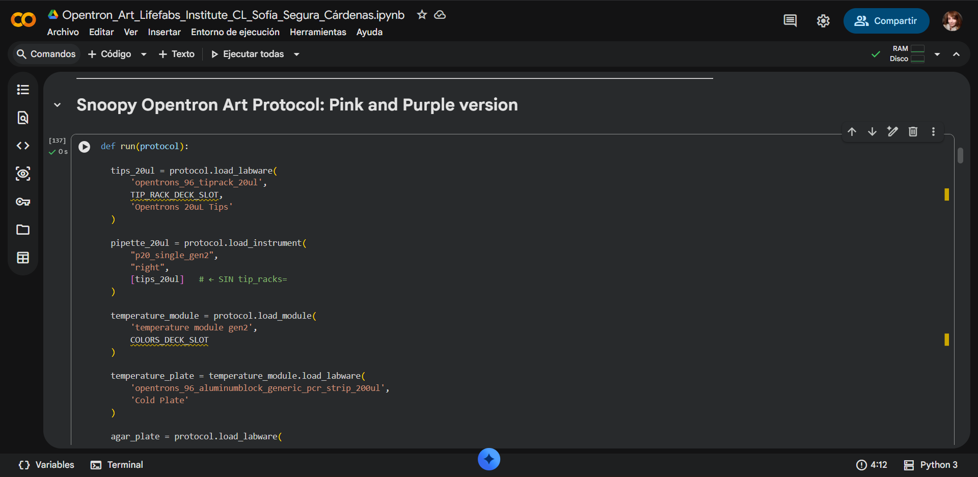
Now, for the code used
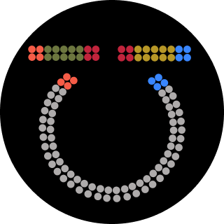
The colors instructed by Lifefabs Institute, London - Node are blue, pink and purple so two versions where made
Link to the Google Colab Opentrons Python notebook: Click here
The final take
Final design in pink and purle (left) and second final design option in blue and pink (right).
4. If the Python component is proving too problematic even with AI and human assistance, download the full Python script from the GUI website and submit that:
Use the download icon pointed to by the red arrow in this diagram.
This are the Python files with the final design downloaded directly from the GUI site:
5. If you use AI to help complete this homework or lab, document how you used AI and which models made contributions.
Did you use AI in to help write your code? If so, what was your experience & which AI tool did you find most helpful?
Did I use AI? For sure! I used AI to help write and optimize my code. I primarily used ChatGPT, which was extremely helpful in reviewing my code, explaining tricky parts, and suggesting optimizations. I also tried Google Colab’s Gemini, but I found its responses less useful and not satisfactory for my needs, even when providing it with access to the code. ChatGPT really guided me step by step, helping me understand how to structure the Opentrons protocol correctly and troubleshoot potential issues, which made the process much smoother and more reliable.
That said, even with ChatGPT’s guidance, we encountered several issues that we were not able to fully resolve, so while it significantly helped improve and clarify the code, it didn’t solve every problem.
Sign up for a robot time slot if you are at MIT/Harvard/Wellesley or at a Node offering Opentrons automation. The Python script you created will be run on the robot to produce your work of art!
At MIT/Harvard? Lab times are on Thursday Feb.19 between 10AM and 6PM.
One of the great parts about having an automated robot is being able to precisely mix, deposit, and run reactions without much intervention, and design and deploy experiments remotely.
1. Find and describe a published paper that utilizes the Opentrons or an automation tool to achieve novel biological applications.
The paper chosen was:
PlasmoTron: an open-source platform for automated culture of malaria parasites.
Sanderson, T. & Rayner, J. C. (2018). PlasmoTron: an open-source platform for automated culture of malaria parasites. Bioarxiv. https://doi.org/10.1101/241596
2. Perspective on Utilizing Foundation Models for Laboratory Automation in Materials Research.
Hatakeyama-Sato, K., Nishida, T., Kitamura, K., et al. (2025). Perspective on Utilizing Foundation Models for Laboratory Automation in Materials Research. Arxiv. arXiv:2506.12312 [cs.RO]. https://doi.org/10.48550/arXiv.2506.12312
3. BOTany Methods: Accessible Automation for Plant Synthetic Biology.
Qiande, M., Lin, A., Larson, L., et al. (2026). BOTany Methods: Accessible Automation for Plant Synthetic Biology. Plant Physiology. https://doi.org/10.1093/plphys/kiag066
Write a description about what you intend to do with automation tools for your final project. You may include example pseudocode, Python scripts, 3D printed holders, a plan for how to use Ginkgo Nebula, and more. You may reference this week’s recitation slide deck for lab automation details.
Example 1: You are creating a custom fabric, and want to deposit art onto specific parts that need to be intertwined in odd ways. You can design a 3D printed holder to attach this fabric to it, and be able to deposit bio art on top. Check out the Opentrons 3D Printing Directory.
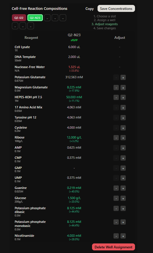
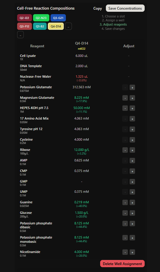
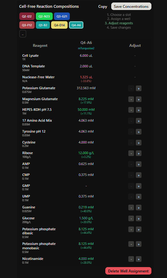
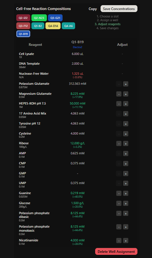
Example 2: You are using the cloud laboratory to screen an array of biosensor constructs that you design, synthesize, and express using cell-free protein synthesis.
Echo transfer biosensor constructs and any required cofactors into specified wells.
Bravo stamp in CPFS reagent master mix into all wells of a 96-well / 384-well plate.
Multiflo dispense the CFPS lysate to all wells to start protein expression.
PlateLoc seal the plate.
Inheco incubate the plate at 37°C while the biosensor proteins are synthesized.
XPeel remove the seal.
PHERAstar measure fluorescence to compare biosensor responses.
I decided to hold on on this section just for the moment since i might change my project this week!
3. Final Project Ideas
Assignees for the following sections
MIT/Harvard students
Required
Committed Listeners
Required
As explained in this week’s recitation, add 1-3 slides in your Node’s section of this slide deck with 3 ideas you have for an Individual Final Project. Be sure to put your name, city, and country on your slide!
The submitted project ideas are as follows:
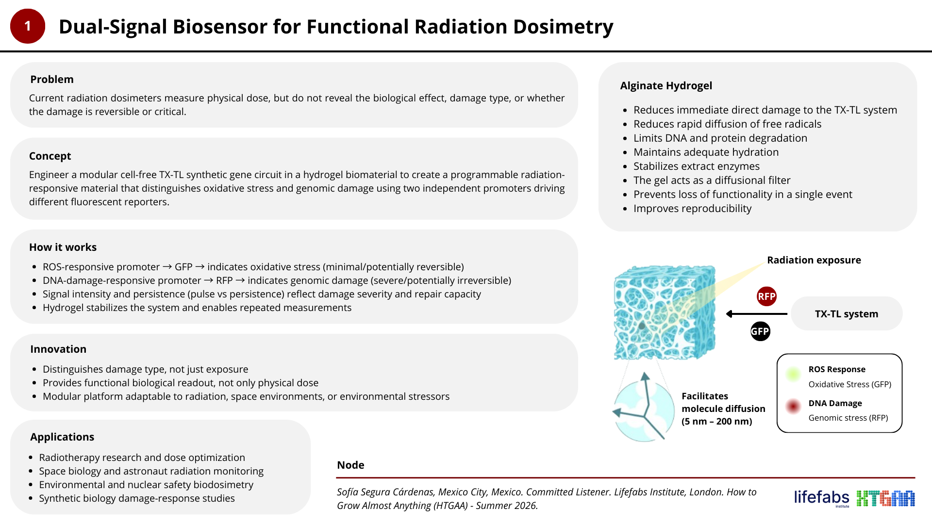
Project N° 1: Dual-Signal Biosensor for Functional Radiation Dosimetry
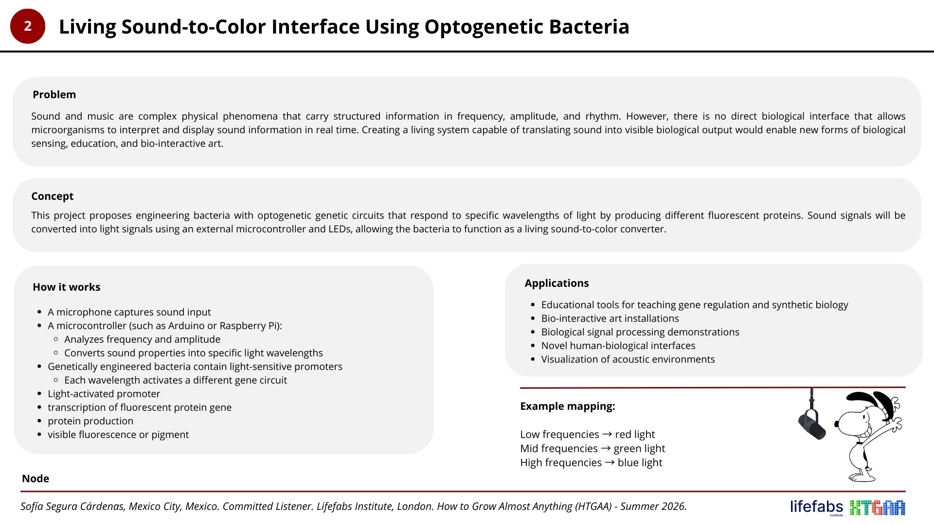
Project N° 2: Living Sound-to-Color Interface Using Optogenetic Bacteria
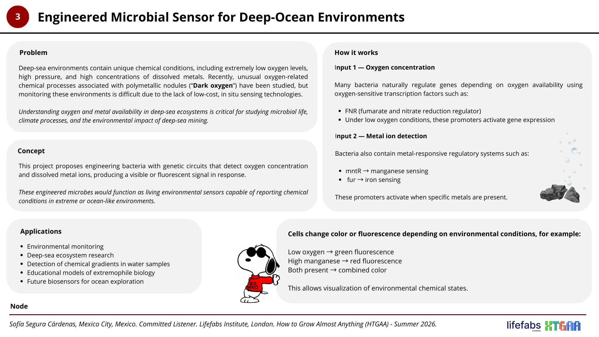
Project N° 3: Engineered Microbial Sensor for Deep-Ocean Environments
You ingest approximately 6.0 × 10²³ amino acid molecules
Final Answer
A 500 g piece of meat contains on the order of:
~ 10²⁴ amino acid molecules
(approximately one mole of amino acids)
Important Notes
This is an order-of-magnitude estimate.
Real proteins are polymers, so their molecular weights are much larger.
The calculation assumes complete digestion into free amino acids.
Water content and protein percentage vary by meat type and preparation.
Interpretation
Eating 500 g of meat means consuming roughly Avogadro-scale molecular quantities of amino acids — on the order of (10²⁴) individual molecules.
This illustrates how biological systems operate at unimaginably large molecular scales, even in everyday nutrition.
2. Why do humans eat beef but do not become a cow, eat fish but do not become fish?
The answer is straightforward: we do not incorporate foreign organisms as whole structures — we digest them into molecular building blocks.
2.1. Digestion breaks macromolecules into basic units
Proteins in beef or fish are large, highly ordered macromolecules. During digestion:
Stomach acid (HCl) denatures proteins.
Proteases such as pepsin, trypsin, and chymotrypsin cleave peptide bonds.
Proteins are hydrolyzed into short peptides and free amino acids.
By the time nutrients are absorbed in the small intestine, the original protein structures no longer exist.
We absorb:
Amino acids
Simple sugars
Fatty acids
Nucleotides
not intact tissues
2.2. Molecular identity is lost during digestion
A cow muscle protein (for example, bovine actin) is not transferred into your muscles as bovine actin. It is broken down into its constituent amino acids:
Your DNA sequence encodes human proteins, not cow or fish proteins.
Therefore:
You rebuild human actin.
You rebuild human collagen.
You rebuild human enzymes.
Your phenotype is determined by your genome, not by the origin of your nutrients.
2.4. Information vs. Matter
This question highlights a fundamental biological principle:
Biological identity is determined by information, not raw material.
Matter (carbon, nitrogen, oxygen, amino acids) is universal. Biological structure depends on how that matter is organized, and organization is encoded in DNA.
Final Answer
Humans do not become cows or fish after eating them because digestion reduces food to molecular building blocks. These building blocks are then reassembled according to human genetic instructions.
We recycle matter — but we do not inherit structural identity from what we eat.
3. Why are there only 20 natural amino acids?
Indeed, why are there only 20 amino acids when the triplet genetic code has 64 codons available? Similarly, could the system work effectively with less than 20? The existence of 20 canonical amino acids is not a chemical inevitability — it is the result of evolutionary optimization. There is no fundamental law of physics that limits proteins to 20 amino acids. Instead, the number reflects a balance between chemical diversity, translational fidelity, and evolutionary stability.
3.1. The genetic code constrains the set
Proteins are encoded by triplet codons:
\[
4^3 = 64 \text{ possible codons}
\]
Out of these:
61 encode amino acids
3 are stop codons
The canonical genetic code maps these 61 codons to 20 amino acids. This mapping is highly redundant (degenerate), which increases robustness against mutations.
Expanding the number of amino acids would require:
New tRNAs
New aminoacyl-tRNA synthetases
Rewiring of codon assignments
This is evolutionarily costly.
3.2. Chemical sufficiency
The 20 amino acids provide a remarkably broad range of chemical functionality:
Nonpolar (hydrophobic packing)
Polar uncharged (hydrogen bonding)
Charged (electrostatics)
Aromatic (π interactions)
Special cases (glycine flexibility, proline rigidity, cysteine disulfide bonding)
With just 20 building blocks, proteins can:
Fold into stable 3D structures
Catalyze diverse chemical reactions
Form dynamic assemblies
Adding many more amino acids would yield diminishing functional returns.
3.3. Evolutionary “freeze” of the code
Once the genetic code became established in early life, it became extremely difficult to change.
This is known as the frozen accident hypothesis:
Once organisms shared a common genetic code, large-scale changes would be lethal.
Thus, the 20 amino acids became locked in by evolutionary history.
3.4. Are there really only 20?
Interestingly, modern biology slightly exceeds 20:
Selenocysteine (21st amino acid)
Pyrrolysine (22nd amino acid)
These are incorporated via special recoding mechanisms.
Additionally, synthetic biology has engineered organisms that incorporate noncanonical amino acids, proving that 20 is not a hard biochemical limit — just the natural evolutionary standard.
Final Answer
There are 20 natural amino acids because evolution selected a chemically sufficient, robust, and efficient set early in the history of life.
The genetic code then became evolutionarily fixed, making large-scale expansion unlikely. The number 20 reflects evolutionary optimization — not chemical necessity.
4. Can you make other non-natural amino acids? Design some new amino acids.
Yes. Non-natural (noncanonical) amino acids can be synthesized chemically and even incorporated into proteins using engineered translation systems.
There is no chemical rule limiting amino acids to the 20 canonical ones. The only strict requirement for incorporation into proteins is that the molecule must:
Contain an α-amino group
Contain an α-carboxyl group
Be compatible with ribosomal geometry
Be recognized by a tRNA / aminoacyl-tRNA synthetase pair
Modern synthetic biology has successfully expanded the genetic code to include dozens of artificial amino acids.
4.1 Design some new amino acids
4.1.1. Design Principles
When designing a new amino acid, we must consider:
Side-chain size and steric compatibility
Polarity and hydrogen bonding capacity
Electronic effects
Stability under physiological conditions
Synthetic accessibility
A) Fluorinated Hydrophobic Amino Acid
Structure Concept:
Replace a methyl group in leucine with a trifluoromethyl group.
Side chain:
\[
-CH_2-CH(CF_3)_2
\]
Purpose:
Increase hydrophobicity
Alter packing interactions
Increase metabolic stability
Fluorinated residues are useful for:
Stabilizing protein cores
Modifying membrane interactions
19F NMR tracking
B) Photo-Crosslinking Amino Acid
Structure Concept:
Attach a diazirine group to a phenylalanine-like ring.
Side chain:
\[
-CH_2-phenyl-diazrine
\]
Purpose:
UV-activated covalent crosslinking
Study protein–protein interactions
Capture transient binding events
This would allow light-controlled structural locking of proteins.
C) Redox-Active Aromatic Amino Acid
Structure Concept:
Modify tyrosine to include a quinone-like moiety.
Side chain:
\[
-CH_2-aromatic-quinone
\]
Purpose:
Electron transfer capability
Catalysis in synthetic enzymes
Bioelectronic interfaces
This could enhance long-range electron transport in engineered proteins.
Are These Realistic?
Yes. Variants of these ideas already exist in synthetic biology:
Fluorinated amino acids
Photo-reactive amino acids
Click-chemistry compatible residues
Redox-active artificial cofactors
Genetic code expansion techniques allow site-specific incorporation using engineered:
Orthogonal tRNA
Engineered aminoacyl-tRNA synthetase
Reassigned stop codons (often UAG)
Final Answer
Yes, non-natural amino acids can be synthesized and incorporated into proteins. The natural 20 amino acids represent an evolutionary standard, not a chemical limit.
By modifying side chains, we can design amino acids with enhanced hydrophobicity, photo-reactivity, redox properties, or catalytic potential — dramatically expanding the functional landscape of proteins.
5. Where did amino acids come from before enzymes that make them, and before life started?
Amino acids did not require life to exist. They can form through purely abiotic chemical processes under the right physical conditions. Before enzymes evolved, amino acids were likely synthesized through prebiotic chemistry on early Earth — and possibly delivered from space.
5.1. Prebiotic Atmospheric Chemistry
In 1953, Stanley Miller and Harold Urey demonstrated that amino acids can form spontaneously from simple gases when energy is supplied.
They simulated early Earth conditions using:
Methane (CH₄)
Ammonia (NH₃)
Hydrogen (H₂)
Water vapor (H₂O)
Electrical sparks (lightning)
After several days, the system produced amino acids such as:
Glycine
Alanine
Aspartic acid
This experiment showed that amino acids can emerge from non-living chemistry.
Another hypothesis suggests that amino acids formed near deep-sea hydrothermal vents.
These environments provide:
Mineral catalysts (iron, nickel sulfides)
Redox gradients
Thermal energy
High pressure
Mineral surfaces may have catalyzed the formation of organic molecules and concentrated them locally.
5.3. Extraterrestrial Delivery
Amino acids have been detected in carbonaceous meteorites, such as the Murchison meteorite.
These findings suggest that:
Amino acids can form in interstellar space
They can survive planetary accretion
Early Earth may have received organic molecules via meteorite bombardment
Thus, part of Earth’s prebiotic inventory may have been extraterrestrial.
5.4. No Enzymes Required
Modern organisms synthesize amino acids using enzyme-catalyzed pathways. However, enzymes are highly evolved catalysts.
Before life:
Chemistry was driven by thermodynamics and energy input
Catalysis may have been mineral-based
Reaction networks were simpler but chemically plausible
Life did not invent amino acids — it inherited them from chemistry.
Final Answer
Amino acids likely originated through abiotic chemical reactions on early Earth (e.g., atmospheric discharge or hydrothermal systems) and possibly through extraterrestrial synthesis. They existed before enzymes because their formation does not require biological catalysis — only appropriate chemical conditions and energy sources.
6. If you make an α-helix using D-amino acids, what handedness (right or left) would you expect?
An α-helix formed from D-amino acids would be left-handed.
6.1. Chirality Determines Helical Handedness
Natural proteins are built from L-amino acids.
When L-amino acids adopt an α-helical conformation, they form a:
Right-handed α-helix
This is the most energetically favorable geometry due to:
Backbone bond angles (φ and ψ)
Steric constraints
Optimal hydrogen bonding alignment
6.2. Mirror Symmetry Argument
D-amino acids are the mirror images of L-amino acids.
Because chirality inverts stereochemistry at the α-carbon, the entire conformational energy landscape is mirrored.
Therefore:
L-amino acids → right-handed α-helix
D-amino acids → left-handed α-helix
The structures are mirror images of each other.
6.3. Hydrogen Bond Geometry
The α-helix is stabilized by hydrogen bonds:
\[
C=O_{(i)} \rightarrow H-N_{(i+4)}
\]
The spatial orientation required for optimal hydrogen bonding depends on backbone stereochemistry.
Switching from L to D reverses:
Dihedral angle preferences
Side-chain orientation
Overall helical twist direction
6.4. Energetics
For L-amino acids:
Right-handed helices are lower in energy.
Left-handed helices are sterically disfavored.
For D-amino acids:
The energetic preference is inverted.
Thus, a D-polypeptide naturally favors a left-handed α-helix.
Final Answer
An α-helix composed entirely of D-amino acids would adopt a left-handed conformation, because reversing chirality at the α-carbon mirrors the backbone geometry and inverts the preferred helical handedness.
8. Why are most molecular helices right-handed?
Most molecular helices in biology are right-handed because life is built almost exclusively from L-amino acids and D-sugars. Molecular chirality determines the preferred helical geometry. Right-handed helices are not universally required by physics — they are a consequence of stereochemistry and evolutionary selection.
8.1. Chirality Bias in Biology
Biological systems exhibit homochirality:
Proteins are built from L-amino acids.
Nucleic acids contain D-ribose or D-deoxyribose.
Because helices emerge from repeating chiral building blocks, their handedness is dictated by the stereochemistry of those monomers.
For example:
L-amino acids → right-handed α-helices
D-sugars → right-handed DNA double helix (B-DNA)
If chirality were inverted, handedness would invert.
8.2. Energetic Favorability
Helical structures form when:
Backbone dihedral angles minimize steric clashes
Hydrogen bonds align optimally
Side chains pack efficiently
For L-amino acids, the lowest-energy α-helical conformation is right-handed. Left-handed helices are possible but typically sterically disfavored in L-polypeptides. Thus, the dominance of right-handed helices reflects energetic optimization under stereochemical constraints.
8.3. Repeating Geometry and Twist
A helix arises from repeating units with constrained bond angles.
Because bond rotations are not symmetric in chiral molecules, the accumulation of small angular preferences results in a macroscopic twist.
Polymers built from D-amino acids form left-handed helices.
Synthetic achiral polymers can form either handedness.
Certain protein segments (e.g., polyproline II helices) may adopt left-handed conformations.
Thus, right-handed dominance in biology reflects molecular asymmetry, not universal physical law.
Final Answer
Most molecular helices in biology are right-handed because they are built from chiral building blocks (L-amino acids and D-sugars) whose stereochemistry favors right-handed twist geometries. Helical handedness emerges from the accumulation of local stereochemical constraints into a global structural bias.
9. Why do β-sheets tend to aggregate?
What is the driving force for β-sheet aggregation?
β-sheets tend to aggregate because their structure exposes hydrogen-bonding backbone groups and often hydrophobic side chains, making intermolecular association energetically favorable.
The driving force is primarily:
Backbone hydrogen bonding
The hydrophobic effect
Reduction of solvent-exposed surface area
Overall free energy minimization
9.1. Backbone Hydrogen Bonding Is Not Fully Satisfied
In an isolated or partially unfolded polypeptide:
Carbonyl (C=O) groups
Amide (N–H) groups
are capable of forming hydrogen bonds. If these groups are not satisfied intramolecularly, they seek partners intermolecularly.
When multiple β-strands align:
\[
C=O_{(i)} \leftrightarrow H-N_{(j)}
\]
They form extended hydrogen-bond networks between molecules. This makes β-sheets particularly prone to forming intermolecular structures.
9.2. The Extended Geometry of β-Strands
β-strands are relatively:
Extended
Planar
Repetitive
This geometry allows:
Easy stacking
Sheet-to-sheet association
Formation of fibrillar structures
Unlike α-helices (which are internally hydrogen-bonded), β-strands expose bonding potential along their length.
9.3. Hydrophobic Effect
Many β-sheet–forming sequences contain hydrophobic residues.
When strands aggregate:
Hydrophobic side chains become buried
Ordered water molecules are released into bulk solvent
Solvent entropy increases
This contributes favorably to:
\[
\Delta G = \Delta H - T\Delta S
\]
The increase in solvent entropy (ΔS > 0) often drives aggregation.
9.4. Structural Complementarity
β-sheets allow:
Tight side-chain interdigitation
Steric zipper formation
Highly ordered packing
This geometric complementarity stabilizes aggregates such as amyloid fibrils.
9.5. Thermodynamic Perspective
Aggregation is favored when:
\[
\Delta G_{aggregation} < 0
\]
This occurs due to:
Enthalpic gain from hydrogen bonding
Entropic gain from water release
Reduced solvent-exposed surface area
Thus, β-sheet aggregation is often thermodynamically favorable, especially at high concentration or under partially denaturing conditions.
Final Answer
β-sheets tend to aggregate because their extended backbone structure allows extensive intermolecular hydrogen bonding and efficient hydrophobic packing. The primary driving forces are backbone hydrogen bonding and the hydrophobic effect, which together lower the system’s free energy and stabilize ordered aggregates.
10. Why do many amyloid diseases form β-sheets?
Can you use amyloid β-sheets as materials?
Many amyloid diseases are associated with β-sheet formation because β-sheets provide a structurally stable, energetically favorable architecture for protein aggregation. The same physical principles that stabilize β-sheets in normal proteins can drive pathological self-assembly under destabilizing conditions.
10.1. Misfolding Exposes Aggregation-Prone Regions
Many proteins contain segments with high β-sheet propensity.
Under normal conditions:
Proteins fold into native conformations
Aggregation-prone regions are buried
However, mutations, oxidative stress, or aging can:
Destabilize native folds
Expose hydrophobic and hydrogen-bonding surfaces
Once exposed, these regions can align into intermolecular β-sheets.
10.2. Cross-β Architecture
Amyloid fibrils share a characteristic structural motif:
β-strands run perpendicular to the fibril axis
Hydrogen bonds run parallel to the fibril axis
This “cross-β” structure creates:
Extensive hydrogen-bond networks
High mechanical stability
Repetitive, ordered packing
Because backbone hydrogen bonds are strong and directional, β-sheets form highly stable fibrillar assemblies.
10.3. Thermodynamic Driving Forces
Amyloid formation is driven by:
Backbone hydrogen bonding
Hydrophobic packing
Release of ordered water (entropy gain)
Reduction of exposed surface area
Thus, amyloid fibrils often represent a deep thermodynamic minimum. In some cases, the amyloid state may be more stable than the native fold.
10.4. Why So Many Diseases?
Examples include:
Alzheimer’s disease
Parkinson’s disease
Huntington’s disease
Prion diseases
In each case, a normally soluble protein adopts an aggregation-prone β-sheet–rich structure. Because β-sheets allow extensive intermolecular stabilization, once nucleation occurs, fibril growth can become self-propagating.
10.5. Can Amyloid β-Sheets Be Used as Materials?
Yes. Although pathological in some contexts, amyloid fibrils have remarkable material properties:
High tensile strength
Nanometer-scale precision
Self-assembly capability
Chemical robustness
Potential applications include:
Biomaterials and scaffolds
Nanowires
Drug delivery systems
Tissue engineering frameworks
Bioelectronic interfaces
Some organisms naturally use functional amyloids (e.g., bacterial biofilms), demonstrating that amyloid structures are not inherently pathological.
Final Answer
Many amyloid diseases form β-sheets because the β-sheet architecture allows extensive intermolecular hydrogen bonding and hydrophobic packing, creating highly stable cross-β fibrils. While pathological in neurodegenerative diseases, amyloid β-sheet assemblies can also be harnessed as robust, self-assembling nanomaterials in biotechnology and materials science.
Part B: Protein Analysis and Visualization
Assignees for the following sections
MIT/Harvard students
Required
Committed Listeners
Required
In this part of the homework, you will be using online resources and 3D visualization software to answer questions about proteins. Pick any protein (from any organism) of your interest that has a 3D structure and answer the following questions:
1. Briefly describe the protein you selected and why you selected it.
I selected the protein RecA from the extremophilic bacterium Deinococcus radiodurans. RecA is a DNA recombination and repair protein that plays a central role in homologous recombination and in the repair of double-strand DNA breaks.
D. radiodurans is known for its extraordinary resistance to ionizing radiation, desiccation, and other extreme environmental stresses. It can survive radiation levels thousands of times higher than those lethal to humans. RecA is essential for this remarkable resilience, as it facilitates DNA strand exchange and genome reassembly after severe DNA fragmentation.
I selected this protein because of its strong relevance to space biology and astrobiology. Radiation is one of the main challenges for life beyond Earth, and understanding the molecular mechanisms that enable DNA repair under extreme radiation conditions provides insight into how life might survive in extraterrestrial environments such as Mars. Additionally, RecA belongs to a highly conserved protein family, making it ideal for evolutionary and structural analysis.
2. Identify the amino acid sequence of your protein.
2.1. How long is it? What is the most frequent amino acid? You can use this Colab notebook to count the frequency of amino acids.
2.2. How many protein sequence homologs are there for your protein? Hint: Use Uniprot’s BLAST tool to search for homologs.
2.3. Does your protein belong to any protein family?
The amino acid sequence was obtainted from UniProt:
Protein lenght: 363 amino acids, wich aligns with the data shown at the UniProt site
Most frecuent amino acid: Alanine (Ala, A), with a Frequency Count of 53 residues (14.60%)
Counting result by Google Colab notebook:
Counting result by JupyterLab:
There was a small error on the second half of the Colab code, but the first part runs without issues. Even with assistance from Gemini AI it was not posible for it to run correctly:
Access to the Google Colab notebook used to count the frequency of amino acids: Click here
Protein sequence homologs: 250 hits found with BLAST
Protein affiliation (family): it belongs to the RecA family
According to UniProt and InterPro classification, RecA belongs to the RecA/Rad51 protein family. This family includes bacterial RecA, archaeal RadA, and eukaryotic Rad51 proteins. These proteins share a conserved ATPase domain of the P-loop NTP-binding superfamily and play essential roles in homologous recombination and DNA repair.
3. Identify the structure page of your protein in RCSB
3.1. When was the structure solved? Is it a good quality structure? Good quality structure is the one with good resolution. Smaller the better (Resolution: 2.70 Å)
3.2. Are there any other molecules in the solved structure apart from protein?
This is considered a good quality crystal structure. In X-ray crystallography, the resolution indicates the level of structural detail observed in the electron density map. Lower values correspond to higher structural precision.
Molecules in the structure:
Yes. According to the RCSB entry, the structure contains additional molecules besides the RecA protein. These include:
ADP (adenosine diphosphate) — a nucleotide bound to the ATPase active site
Magnesium ion (Mg²⁺) — a cofactor required for nucleotide binding and ATP hydrolysis
Water molecules (HOH) — commonly observed in crystal structures
These molecules are functionally relevant because RecA is an ATPase, and nucleotide binding plays an important role in its mechanism during DNA repair and homologous recombination.
Protein affiliation:
Yes. According to the SCOP structural classification database, the protein belongs to the following hierarchy:
Fold:RecA-like classic
Superfamily:RecA-like P-loop NTPases
Family:RecA/Rad51/KaiC-like ATPases
SCOP ID:4004007
This classification groups proteins with similar three-dimensional folds and ATPase domains, even if their sequences differ. Members of this superfamily share a conserved P-loop NTP-binding domain involved in nucleotide binding and hydrolysis.
4. Open the structure of your protein in any 3D molecule visualization software:
PyMol Tutorial Here (hint: ChatGPT is good at PyMol commands)
Visualize the protein as “cartoon”, “ribbon” and “ball and stick”.
Color the protein by secondary structure. Does it have more helices or sheets?
Color the protein by residue type. What can you tell about the distribution of hydrophobic vs hydrophilic residues?
Visualize the surface of the protein. Does it have any “holes” (aka binding pockets)?
Protein visualization in PyMOL:
Cartoon
Ribbon
Ball and Stick
Helices or Sheets?
🔴 α-helices 🟡 β-sheets 🟢 loops or flexible regions
Cartoon:
The cartoon representation highlights the secondary structure elements of the protein. The structure contains several α-helices and a smaller number of β-sheets arranged near the center of the protein. Overall, α-helices appear to be more abundant than β-sheets.
Ribbon:
The ribbon representation reveals the overall fold of the protein. The structure consists of a central β-sheet region surrounded by α-helices, which is characteristic of the RecA-like fold found in ATP-binding proteins.
Ball and Stick:
The ball-and-stick representation shows the detailed atomic arrangement of the amino acid residues. Hydrophobic residues appear mostly buried within the protein core, whereas hydrophilic residues are more exposed on the surface, which is typical for soluble cytoplasmic proteins.
Hydrophobic vs Hydrophilic
Hydrophobic residues tend to cluster within the interior of the protein structure, while hydrophilic and charged residues are more exposed on the protein surface, which is typical for soluble proteins interacting with the aqueous cytoplasm.
Surface representation of the protein reveals several small cavities distributed across the structure. These cavities likely correspond to potential ligand-binding pockets. In RecA proteins, such pockets are typically involved in nucleotide binding (ATP/ADP), which is required for DNA repair activity.
Part C. Using ML-Based Protein Design Tools
Assignees for the following sections
MIT/Harvard students
Required
Committed Listeners
Required
In this section, we will learn about the capabilities of modern protein AI models and test some of them in your chosen protein.
Use ESM2 to generate an unsupervised deep mutational scan of your protein based on language model likelihoods.
The deep mutational scan generated using the protein language model ESM-2 evaluates how likely each amino-acid substitution is at every position in the protein sequence of RecA.
In the Heatmap:
The x-axis represents the position of residues in the protein sequence.
The y-axis represents the amino acid substituted at that position.
Each cell corresponds to a single mutation.
The color scale represents the model score, which reflects how compatible a mutation is with the learned evolutionary patterns of proteins.
Color
Score Range
Interpretation
🟡 Yellow
Positive (>0)
Favorable or tolerated mutation
🟢 Green
Around 0
Neutral mutation
🔵 Blue
Moderately negative
Likely destabilizing mutation
🟣 Purple
Very negative (< -8)
Strongly deleterious mutation
Mutations with strongly negative scores are predicted to be highly disruptive to the protein structure or function.
Can you explain any particular pattern? (choose a residue and a mutation that stands out)
One of the most noticeable patterns in the heatmap is the presence of vertical dark bands across several sequence positions. These vertical bands indicate positions that are highly sensitive to mutation, where almost any substitution results in a strongly negative score. This pattern suggests that these residues are evolutionarily conserved and structurally or functionally important.
In proteins such as RecA, highly conserved residues often correspond to:
Catalytic residues
ATP-binding residues
Residues located in the structural core of the protein
Mutations at these positions are therefore predicted to disrupt protein folding or functional activity.
Strongly unfavorable mutations
a) Cysteine mutations
A particularly prominent pattern in the heatmap corresponds to mutations to cysteine (C), which frequently show very negative scores across many sequence positions. Introducing cysteine residues can be problematic for several reasons:
Disulfide bond formation: Cysteine residues can form disulfide bonds, which may introduce unintended cross-links that disrupt the protein’s native structure.
Structural constraints: Cysteine has a reactive thiol group that may interfere with local interactions within the protein core.
Protein environment mismatch: In cytosolic proteins such as RecA, cysteines are relatively rare and often occur only at specific functional sites.
Because of these factors, many cysteine substitutions are predicted to be structurally destabilizing, which explains the strong negative scores observed in the heatmap.
b) Tryptophan mutations
Another notable pattern is the strong negative scores observed for mutations to tryptophan (W) at many positions. Tryptophan is the largest amino acid, and its bulky aromatic side chain can disrupt tightly packed regions of the protein structure. When introduced at positions that cannot accommodate large residues, it may:
Create steric clashes
Disturb secondary structure packing
Destabilize the hydrophobic core
As a result, many tryptophan substitutions receive very negative model scores, indicating that these mutations are likely to be deleterious.
Favorable or tolerated mutations
Some amino acids show mostly neutral or favorable scores across the sequence. One example in the heatmap is serine (S), which appears largely green and occasionally yellow. Serine substitutions are often tolerated because:
it is small in size
it is polar but not strongly charged
it can participate in hydrogen bonding
it does not introduce major steric clashes
Because of these properties, serine can frequently replace other small or polar residues without significantly disrupting the protein structure.
Neutral mutations
Neutral mutations (shown in green) typically occur when the substituted amino acid has similar physicochemical properties to the original residue. Examples include substitutions between:
Hydrophobic residues (e.g., V → I)
Polar residues (e.g., S → T)
Similarly sized amino acids
These mutations tend to preserve the overall structural stability and local interactions of the protein.
C1.2. Latent space analysis
Use the provided sequence dataset to embed proteins in reduced dimensionality.
Analyze the different formed neighborhoods: do they approximate similar proteins?
Place your protein in the resulting map and explain its position and similarity to its neighbors.
The following dimensionality reduction technique preserves local similarity relationships, allowing sequences with similar structural or evolutionary features to cluster together in the resulting latent space.
NOTE
Some adjusments were made. During the latent space analysis, an error occurred while applying the t-SNE dimensionality reduction using scikit-learn. The program returned the message ValueError: perplexity must be less than n_samples. This error arose because the input dataset initially contained only a single protein sequence corresponding to RecA from Deinococcus radiodurans. The t-SNE algorithm requires multiple samples to estimate neighborhood relationships between points, and the perplexity parameter (set to 30) must always be smaller than the number of samples in the dataset. Because only one sequence was provided, the algorithm could not compute the embedding. The issue was resolved with assistance from Gemini, which identified that the FASTA input needed multiple sequences. The original FASTA link was therefore replaced with a dataset containing 50 homologous protein sequences related to RecA, allowing the model to generate valid embeddings and complete the latent space analysis.
With error
Fixed
Final take
The following color encoding helps visualize how proteins are distributed along the third dimension of the latent space and highlights subtle structural relationships that may not be obvious from spatial position alone.
Color
TSNE3 Value
Interpretation
🔵 Dark purple
Low values (negative)
Proteins positioned in lower regions of the latent dimension
🟣 Magenta / 🩷 pink
Intermediate values
Proteins occupying middle regions of the embedding
🟠 Orange / 🟡 yellow
High values (positive)
Proteins separated along the third dimension
NOTE: The color scale represents the TSNE3 coordinate and does not indicate protein quality or functional superiority. Instead, it simply reflects the relative position of proteins along the third dimension of the embedding space.
a) Neighborhood structure in the embedding space
The resulting 3D visualization reveals a clear clustering pattern, where the majority of sequences form a dense neighborhood in the latent space. This clustering indicates that many sequences in the dataset share similar sequence patterns, structural motifs, or evolutionary relationships, and likely belong to related protein families or structural classes. Protein language models capture evolutionary constraints during training, meaning sequences with similar functional or structural properties tend to occupy nearby regions in the embedding space.
Within the visualization, most sequences form a compact cluster, suggesting they share significant sequence similarity and may belong to related recombination or DNA-binding protein families.
b) Outlier sequences
A small number of sequences appear separated from the main cluster, forming outliers in the latent space. These outliers may correspond to proteins that:
Contain significant sequence divergence
Belong to more distant homologous families
Contain additional domains or structural insertions
Protein language models often place functionally related but evolutionarily distant proteins in nearby regions, but sequences that diverge significantly may appear as isolated points in the reduced dimensional space.
Placement of the selected protein
RecA from Deinococcus radiodurans, appears within the main cluster of sequences in the embedding space. Its coordinates (TSNE1 ≈ −39, TSNE2 ≈ −5, TSNE3 ≈ −0.5) place it close to several other proteins in the dataset. The surrounding points share similar color and spatial proximity, indicating that these proteins have similar embedding representations.
C2. Protein Folding
1. Fold your protein with ESMFold. Do the predicted coordinates match your original structure?
ESMFOLDING RESULTS
Using device: cuda:0
Total sequence length: 363
Running ESMFold inference for sequence with length 363...
Prediction complete. ptm: 0.919 plddt: 94.831
Results saved to RecA_5fccb/
CPU times: user 45.5 s, sys: 8.63 s, total: 54.1 s
Wall time: 1min 24s
Displays
a) Sidechain
b) Mainchain
c) Sidechain + Mainchain
Comparison
Overall, they do look similar 😃! The structure predicted with ESMFold closely resembles the monomeric fold of the RecA proteins reported in experimental structures and AlphaFold models on UniProt. The predicted structure contains the characteristic α/β core domain and several α-helices typical of RecA family proteins. However, it does not reproduce the circular oligomeric structure observed in some UniProt models (PDB 1XP8), because those structures represent multimeric assemblies composed of several RecA subunits. ESMFold predicts the structure of a single polypeptide chain (monomer), which explains why the predicted structure resembles monomeric crystal structures such as 2ofo.1 rather than the oligomeric filament assemblies (1xp8.1.F).
SWISS-MODEL homology model based on template AlphaFold: AF-P42443-F1.
RecA structure predicted using ESMFold.
The RecA structure predicted with ESMFold showed a very high confidence score (pLDDT = 94.83) and was compared with previously available structural models, including the SWISS-MODEL homology model based on the crystal structure 2ofo.1 (QMEANDisCo = 0.77 ± 0.05) and the AlphaFold prediction AF-P42443-F1 (average pLDDT = 88.88). All models display the characteristic RecA fold, consisting of a central α/β ATPase domain with a β-sheet core surrounded by multiple α-helices. The arrangement of secondary structural elements, including β-strands, α-helices, and connecting loops, is largely conserved between the three structures. Minor differences are mainly observed in flexible regions such as loops and the C-terminal tail, which are known to exhibit conformational variability. Overall, the high pLDDT value obtained with ESMFold indicates that the predicted structure is highly reliable and consistent with experimentally derived and AI-predicted RecA models.
2. Try changing the sequence, first try some mutations, then large segments. Is your protein structure resilient to mutations?
C3. Protein Generation
Inverse-Folding a protein: Let’s now use the backbone of your chosen PDB to propose sequence candidates via ProteinMPNN
Analyze the predicted sequence probabilities and compare the predicted sequence vs the original one.
Input this sequence into ESMFold and compare the predicted structure to your original.
The “New Sequence” generated by ProteinMPNN is not merely a mutated version of the original; it’s a de novo design tailored for the provided 3D protein structure (PDB 1XP8). ProteinMPNN operates on the principle of inverse protein folding, where instead of predicting the 3D structure from a given amino acid sequence, it takes a fixed 3D backbone and designs an amino acid sequence that is predicted to be compatible with and stable within that structure.
How the new sequence is generated
1. Structural Input: The model uses the atomic coordinates of the protein backbone (from PDB 1XP8) as its primary input.
2. Per-Position Probability: For each amino acid position along the chain, ProteinMPNN evaluates the local structural environment (neighboring residues, local geometry). Based on this context, it predicts a probability distribution over all 20 standard amino acids (and sometimes ‘X’ for ambiguous or masked regions) for that specific position.
3. Sampling: A new amino acid is then sampled from this probability distribution for each position. The sampling_temp parameter (set to 0.1 in our run) influences this sampling: a lower temperature means the model is more likely to pick the highest-probability amino acid, leading to more conservative designs, while a higher temperature introduces more diversity.
4. Novelty and Mutations: The resulting “New Sequence” is thus a sequence that ProteinMPNN predicts will stably adopt the input 3D conformation. Differences between this generated sequence and the “Native Sequence” (from the original PDB) represent designed mutations. These mutations aim to optimize the sequence for the given fold, potentially improving stability or introducing new functions.
Amino acid probability map
Each row on the y-axis represents a different amino acid, and each column on the x-axis corresponds to a specific position in the protein sequence. The color intensity at each cell (intersection of an amino acid and a position) indicates the average probability that ProteinMPNN assigned to that amino acid at that position.
Interpretation
Hotter/Brighter Colors (yellow, white): Indicate a high probability for that specific amino acid at that particular position. This suggests that the model strongly prefers or predicts that amino acid to be structurally compatible at that site. These positions are often critical for the protein’s fold or function, or simply have strong local preferences.
Colder/Darker Colors (blue, purple): Indicate a low probability for that amino acid at that position. The model considers these amino acids unlikely or incompatible with the structural context of that site.
Vertical Stripes of Hot Colors: If a column (a specific position) shows a very bright stripe concentrated on one or a few amino acids, it means that position is highly constrained or conserved. The model has a very strong preference for only a few types of amino acids there.
Horizontal Stripes/Scattered Hot Colors: If a position has several amino acids with moderately high probabilities, it suggests more variability or plasticity at that site. The structure can tolerate different amino acids there.
The “New Sequence” is derived from these probability distributions. The amino acid selected for each position in the new sequence would typically be one of the high-probability amino acids shown in the heatmap for that specific position, especially with a low sampling_temp.
New Sequence:GELAALLERLARALLWAANGPGAAYAPDERAGLPVEVVPTGVVSLDRALGVGGLPKGRITLIQGPPGSGKTTLALQVVAEAQRAGGKAALIDMEGELDEARAAALGVDVAALERYRPENGEEALEKTLELVSSGEYDVVVIDSLQAAVPKAELXXXXXXXXAGLRAELFARYLARLKEVLAGTGTCLIILHHTXXXXXXXXXXXXXXXGIEAVREAASVILDVRRVGEPEXXXXXXRSWRVEIRVVKNTVAPAGRSVVVTLTEGEGFDRIADLVEEAARLGIIERDGNKYSYKNKFIGEGEKAAAATIAKDPALEEEIRREVLERIR
Part D. Group Brainstorm on Bacteriophage Engineering
Assignees for the following sections
MIT/Harvard students
Optional
Committed Listeners
Required
Find a group of ~3–4 students
Read through the Phage Reading material listed under “Reading & Resources” below.
Review the Bacteriophage Final Project Goals for engineering the L Protein:
Increased stability (easiest)
Higher titers (medium)
Higher toxicity of lysis protein (hard)
Brainstorm Session
Choose one or two main goals from the list that you think you can address computationally (e.g., “We’ll try to stabilize the lysis protein,” or “We’ll attempt to disrupt its interaction with E. coli DnaJ.”).
Write a 1-page proposal (bullet points or short paragraphs) describing:
Which tools/approaches from recitation you propose using (e.g., “Use Protein Language Models to do in silico mutagenesis, then AlphaFold-Multimer to check complexes.”).
Why do you think those tools might help solve your chosen sub-problem?
Name one or two potential pitfalls (e.g., “We lack enough training data on phage–bacteria interactions.”).
Nelson, D. L., & Cox, M. M. (2021). Lehninger Principles of Biochemistry (8th ed.). W.H. Freeman.
Hall, J. E. (2020). Guyton and Hall Textbook of Medical Physiology (14th ed.). Elsevier.
Alberts, B. et al. (2022). Molecular Biology of the Cell (7th ed.). Garland Science.
Crick, F. H. C. (1968). The origin of the genetic code. Journal of Molecular Biology, 38(3), 367–379.
Liu, C. C., & Schultz, P. G. (2010). Adding new chemistries to the genetic code. Annual Review of Biochemistry, 79, 413–444.
Lobanov, A. V., et al. (2009). Selenocysteine: The 21st amino acid. Journal of Biological Chemistry, 284(44), 28532–28536.
Weber, A.L., Miller, S.L. Reasons for the occurrence of the twenty coded protein amino acids. J Mol Evol 17, 273–284 (1981). https://doi.org/10.1007/BF01795749
Doig, A.J. (2017), Frozen, but no accident – why the 20 standard amino acids were selected. FEBS J, 284: 1296-1305. https://doi.org/10.1111/febs.13982
Young, Travis S. & Schultz, P. G. schultz@scripps.edu. (April, 2010). Beyond the Canonical 20 Amino Acids: Expanding the Genetic Lexicon. Journal of Biological Chemistry, Volume 285, Issue 15, 11039 - 11044. https://doi.org/10.1074/jbc.R109.091306
Miles, S. A., Nillama, J. A., & Hunter, L. (2023). Tinker, Tailor, Soldier, Spy: The Diverse Roles That Fluorine Can Play within Amino Acid Side Chains. Molecules, 28(17), 6192. https://doi.org/10.3390/molecules28176192
Lee, Hyang-Yeol; Lee, Kyung-Hoon; Al-Hashimi, Hashim M.; Marsh, E. Neil G. . (2006). Modulating Protein Structure with Fluorous Amino Acids: Increased Stability and Native-like Structure Conferred on a 4-Helix Bundle Protein by Hexafluoroleucine. Journal of the American Chemical Society, 128(1), 337–343. doi:10.1021/ja0563410
Buer, B.C. and Marsh, E.N.G. (2012), Fluorine: A new element in protein design. Protein Science, 21: 453-462. https://doi.org/10.1002/pro.2030
Benjamin C. Buer; E. Neil G. Marsh. (2012). Fluorine: A new element in protein design. , 21(4), 453–462. doi:10.1002/pro.2030
Buer, B.C., Meagher, J.L., Stuckey, J.A. & Marsh, E.N.G. (2012). Structural basis for the enhanced stability of highly fluorinated proteins, Proc. Natl. Acad. Sci. U.S.A. 109 (13) 4810-4815. https://doi.org/10.1073/pnas.1120112109
Costantino, A., Pham, L.B.T., Barbieri, L., Calderone, V., Ben-Nissan, G., Sharon, M., et al. Controlling the incorporation of fluorinated amino acids in human cells and its structural impact. Protein Science. 2024; 33(3):e4910. https://doi.org/10.1002/pro.4910
Zhang, Huimin; Song, Yanling; Zou, Yuan; Ge, Yun; An, Yuan; Ma, Yanli; Zhu, Zhi; Yang, Chaoyong James . (2014). A diazirine-based photoaffinity probe for facile and efficient aptamer–protein covalent conjugation. Chemical Communications, 50(38), 4891–. doi:10.1039/c4cc01528b
S. Ravindra, C. P. Irfana Jesin, A. Shabashini, G. C. Nandi. (2021). Recent Advances in the Preparations and Synthetic Applications of Oxaziridines and Diaziridines. Catal. 363, 1756. https://doi.org/10.1002/adsc.202001372
Famiano, M.A., Boyd, R.N., Kajino, T. et al. Amino Acid Chiral Selection Via Weak Interactions in Stellar Environments: Implications for the Origin of Life. Sci Rep 8, 8833 (2018). https://doi.org/10.1038/s41598-018-27110-z
Ronald Breslow,
The origin of homochirality in amino acids and sugars on prebiotic earth. Tetrahedron Letters, Volume 52, Issue 32, 2011, Pages 4228-4232, ISSN 0040-4039. https://doi.org/10.1016/j.tetlet.2011.06.002
NGLViewer: NGL Viewer is a collection of tools for web-based molecular graphics. WebGL is employed to display molecules like proteins and DNA/RNA with a variety of representations.
Chimera: A highly extensible program for interactive visualization and analysis of molecular structures and related data, including density maps, supramolecular assemblies, sequence alignments, docking results, trajectories, and conformational ensembles.
Superoxide dismutase 1 (SOD1) is a cytosolic antioxidant enzyme that converts superoxide radicals into hydrogen peroxide and oxygen. In its native state, it forms a stable homodimer and binds copper and zinc.
Mutations in SOD1 cause familial Amyotrophic Lateral Sclerosis (ALS). Among them, the A4V mutation (Alanine → Valine at residue 4) leads to one of the most aggressive forms of the disease. The mutation subtly destabilizes the N-terminus, perturbs folding energetics, and promotes toxic aggregation.
Challenge:
Design short peptides that bind mutant SOD1.
Then decide which ones are worth advancing toward therapy.
Available models:
PepMLM: target sequence-conditioned peptide generation via masked language modeling
MATK A VCVLKGDGPVQGIINFEQKESNGPVKVWGSIKGLTEGLHGFHVHEFGDNTAGCTSAGPHFNPLSRKHGGPKDEERHVGDLGNVTADKDGVADVSIEDSVISLSGDHCIIGRTLVVHEKADDLGKGGNEESTKTGNAGSRLACGVIGIAQ
MATK V VCVLKGDGPVQGIINFEQKESNGPVKVWGSIKGLTEGLHGFHVHEFGDNTAGCTSAGPHFNPLSRKHGGPKDEERHVGDLGNVTADKDGVADVSIEDSVISLSGDHCIIGRTLVVHEKADDLGKGGNEESTKTGNAGSRLACGVIGIAQ
The list of the 16 generated peptides and the 17 one added for control:
PepMLM assigns a pseudo-perplexity score to each generated peptide, reflecting the model’s confidence in the sequence given the target protein context. Lower pseudo-perplexity values indicate higher model confidence and a better fit to the learned sequence distribution of potential binders.
Index
Binder
Pseudo Perplexity
X
0
WRYYATAVEHKX
10.445826
Yes
1
WRYYAVAVRHKX
12.354167
Yes
2
WRYPVVALALKE
11.448351
No
3
HRYGATVVAWKE
11.524772
No
4
WRYYAAALEHGX
8.100808
Yes
5
WLYYAAALRHKX
15.539718
Yes
6
HHSYPVALEHWK
14.301987
No
7
HHYYAVAAAWKK
13.441748
No
8
WRSGPVAARWWX
8.107713
Yes
9
WLYGATGAAHGE
9.124785
No
10
WLYPAVAAELKX
9.295740
Yes
11
WLYPVTVLELKE
19.095537
No
12
WLYPVVALAHGX
10.353661
Yes
13
WLYGAAAVEWGE
14.981852
No
14
WHYGAAAVRWKX
10.837565
Yes
15
HRYPAVAVRHGX
12.434339
Yes
16
FLYRWLPSRRGG
N/A
No
Several generated peptides contain the residue X, which represents an ambiguous or unknown amino acid in protein sequence notation. In peptide design workflows, X typically appears when the model has uncertainty about the most probable residue at that position. Because X cannot be synthesized or interpreted structurally, these peptides are generally considered lower-confidence candidates for downstream therapeutic design and may be deprioritized in later filtering steps.
Observed sequence pattern
Many of the generated peptides begin with W, H, or the motif WR. Examples include sequences such as WRYY…, WLY…, and HRY…. This pattern suggests that PepMLM may have identified an aromatic and positively charged motif favorable for interaction with SOD1.
A possible explanation is related to the chemical properties of these residues:
W (Tryptophan) can participate in hydrophobic and aromatic interactions, which often stabilize protein–peptide binding interfaces.
R, H, and K (Arginine, Histidine, Lysine) are positively charged residues that can contribute to electrostatic interactions with negatively charged regions on the protein surface.
Together, these features may help promote stable binding between the designed peptides and the mutant SOD1 protein.
Selection of the four best candidate peptides
To select candidates for further evaluation, peptides were prioritized based on:
Low pseudo-perplexity scores (higher model confidence)
Absence of ambiguous residues (X)
Reasonable sequence composition for peptide stability
Peptide
Pseudo Perplexity
Justification
WLYGATGAAHGE
9.1248
Lowest perplexity among sequences without ambiguous residues; strong model confidence.
WRYPVVALALKE
11.4484
Moderate perplexity and no ambiguous residues; hydrophobic core may favor binding.
HRYGATVVAWKE
11.5248
Balanced composition with aromatic and hydrophobic residues that may stabilize interactions.
HHSYPVALEHWK
14.3020
Slightly higher perplexity but still valid; contains aromatic and charged residues that could support binding.
For each peptide, submit the mutant SOD1 sequence followed by the peptide sequence as separate chains to model the protein-peptide complex.
Record the ipTM score and describe where the peptide appears to bind. Does it localize near the N-terminus where A4V sits? Does it engage the β-barrel region or approach the dimer interface? Does it appear surface-bound or partially buried?
Describe the ipTM values you observe and whether any PepMLM-generated peptide matches or exceeds the known binder.
All AlphaFold predictions were run using a fixed random seed [100] to ensure reproducibility across peptide–protein complex predictions.
Run 1: WLYGATGAAHGE
Parameters
Run 1
(ipTM=0.49, pTM=0.83)
In the structure:
SOD1 appears dark blue, meaning the protein structure is predicted with very high confidence.
The peptide is yellow/orange, meaning low confidence in its position and structure.
This usually indicates that AlphaFold is uncertain about the peptide’s binding pose, which is consistent with your ipTM = 0.49.
The peptide WLYGATGAAHGE produced an ipTM score of 0.49, indicating very low confidence in the predicted protein–peptide interaction. The overall structure of SOD1 was predicted with high confidence (dark blue pLDDT values), while the peptide displayed lower confidence scores (yellow/orange). Structural inspection shows the peptide positioned along the surface of the SOD1 β-barrel, rather than binding near the N-terminal region where the A4V mutation is located. The low pLDDT values suggest that the peptide adopts a flexible or weakly defined binding conformation, consistent with a surface-associated interaction rather than a tightly bound interface.
Does it localize near the N-terminus where A4V sits?
No. The peptide does not appear to bind near the N-terminal region where the A4V mutation is located. Instead, it is positioned further along the side of the protein.
Does it engage the β-barrel region or approach the dimer interface?
Yes. The peptide is located along the surface of the SOD1 β-barrel, which is the central structural feature of the protein composed of several β-strands (the arrow-shaped ribbons in the structure). This suggests a surface interaction with the β-barrel region.
No. The model shows only a single SOD1 monomer, so the dimer interface is not present in this prediction. Therefore, the peptide cannot be interacting with the dimer interface in this model.
Does it appear surface-bound or partially buried?
It appears surface-associated but weakly constrained. The peptide is positioned near the surface of the protein, but the yellow/orange coloring indicates low structural confidence, meaning AlphaFold is not strongly confident about the exact binding pose. This suggests that the peptide may transiently interact with the protein surface rather than forming a stable, well-defined interface.
pTM also decreased (0.83 → 0.80) → more structural perturbation in SOD1
Important observation: protein color changes
The protein is no longer uniformly dark blue. This suggests:
Local decreases in pLDDT
Possible structural perturbations induced by the peptide
The peptide may be destabilizing local regions of SOD1 or AlphaFold is uncertain about the interface, propagating uncertainty into nearby residues. A peptide can appear to interact more broadly but still produce lower confidence, indicating a less stable or more disruptive interaction.
The peptide WRYPVVALALKE produced an ipTM score of 0.43, indicating moderate but still low confidence in the predicted protein–peptide interface. The peptide appears to align along the surface of the β-barrel, forming broader contact with the protein compared to the first design. However, it does not localize near the N-terminal region where the A4V mutation resides, and no interaction with the dimer interface can be assessed. The peptide shows partial structural definition, with a central region of moderate confidence and flexible termini. Notably, the SOD1 structure exhibits localized decreases in confidence, suggesting possible structural perturbation or uncertainty induced by the peptide. Overall, the interaction appears surface-bound and weakly defined, without a clear binding pocket or stable interface.
Does it localize near the N-terminus where A4V sits?
No, not clearly. The peptide is positioned along the side of the β-barrel, not near the top region where the N-terminus (and A4V mutation) is located. Therefore, it does not appear to target the mutation site directly.
Does it engage the β-barrel region or approach the dimer interface?
Yes, more convincingly than Run 1. The peptide runs along the surface of the β-sheets, appearing to align with the β-barrel architecture. This suggests a surface-guided interaction, possibly stabilized by:
hydrophobic residues (V, L, A)
aromatic residue (W, Y)
However, it still does not insert into a defined binding pocket.
No. Again, only a monomer is modeled, so the dimer interface is absent. No conclusions can be drawn about dimer stabilization.
Does it appear surface-bound or partially buried?
Partially surface-bound, partially flexible. The central region of the peptide (yellow) suggests moderate confidence (~70 pLDDT). The ends (orange) remain highly flexible/unresolved. This indicates:
Some transient or weak interaction with the protein surface
No stable, well-defined binding conformation
Run 3: HRYGATVVAWKE
Parameters
Run 3
(ipTM=0.26, pTM=0.87)
The protein is predicted extremely well
The peptide is not interacting meaningfully at all
The peptide HRYGATVVAWKE produced an ipTM score of 0.26, indicating very low confidence in the predicted protein–peptide interaction, while the overall SOD1 structure was predicted with high confidence (pTM = 0.87). The peptide appears completely detached from the protein, with no visible interaction with the β-barrel or any defined binding region. It does not localize near the N-terminal region where the A4V mutation is located, and no interaction with the dimer interface can be assessed. The peptide exhibits very low confidence (orange coloring) across most of its length, suggesting high flexibility and lack of a stable conformation. Overall, this model indicates no meaningful binding interaction, representing the weakest candidate among the peptides tested.
Does it localize near the N-terminus where A4V sits?
No. The peptide is located far from the N-terminal region of SOD1. It does not approach the top portion of the structure where the A4V mutation resides.
Does it engage the β-barrel region or approach the dimer interface?
No. Unlike Run 2, this peptide does not even align along the β-barrel surface. It is clearly spatially separated from the structured core of the protein.
No. Again, only a monomer is modeled, so the dimer interface is not present.
Does it appear surface-bound or partially buried?
Completely detached, his is actually the cleanest negative result so far! This are the key observation:
The peptide is far away from the protein
It is colored mostly orange, indicating very low confidence and high flexibility
There is no visible interaction interface
This is essentially a non-binding prediction.
Why this happens
Even though the sequence contains:
H (charged)
W/Y (aromatic)
hydrophobic residues (V, A)
The arrangement and context of residues matters more than composition. This peptide likely does not form a compatible interface geometry, remains too flexible to stabilize binding or is treated by AlphaFold as an independent chain.
Run 4: HHSYPVALEHWK
Parameters
Run 4
(ipTM=0.27, pTM=0.87)
Same pattern as Run 3:
Protein is very well predicted
Interaction is essentially absent
Important observation: peptide secondary structure
The peptide looks “thicker” and more structured (helix-like or sheet-like), it may be forming a transient secondary structure (likely α-helix). However, internal folding ≠ binding. This means, the peptide can stabilize itself but still fails to interact with SOD1.
This suggests: Binding requires complementarity, not just structure.
Even with:
aromatic residues (Y, W)
charged residues (H)
The peptide does not match the geometry or chemistry of the binding surface.
The peptide HHSYPVALEHWK produced an ipTM score of 0.27, indicating very low confidence in the predicted protein–peptide interaction, while the SOD1 structure was predicted with high confidence (pTM = 0.87). The peptide appears fully detached from the protein, with no observable interaction with the β-barrel or the N-terminal region containing the A4V mutation. Interestingly, unlike other non-binding peptides, this sequence adopts a more compact and partially structured conformation, suggesting the formation of internal secondary structure. Despite this, the peptide does not form a stable interface with SOD1, indicating that self-folding alone is insufficient for binding. Overall, this model represents a non-binding case with increased peptide structural definition.
Does it localize near the N-terminus where A4V sits?
No. The peptide is clearly distant from the N-terminal region and does not approach the area where the A4V mutation is located.
Does it engage the β-barrel region or approach the dimer interface?
No. There is no contact with the β-barrel surface. The peptide is positioned away from the structured core of the protein.
No. As in all previous runs, only a monomer is modeled, so the dimer interface is not represented.
Does it appear surface-bound or partially buried?
Detached, but structurally more defined than previous cases. This is the key difference:
The peptide is still far from the protein (no interaction)
But unlike Run 3, it is not just a random flexible chain
It appears to form a more compact, partially folded structure
Run 5: FLYRWLPSRRGG
Parameters
Run 5
(ipTM=0.30, pTM=0.78)
The protein structure is still predicted well, but the interaction between the peptide and SOD1 is predicted very poorly!
The control peptide FLYRWLPSRRGG produced an ipTM score of 0.30, indicating very low confidence in the predicted protein–peptide interface. While the overall fold of SOD1 was predicted with reasonable confidence (pTM = 0.78), the peptide displayed very low pLDDT values across its entire length, suggesting high structural uncertainty. Visual inspection shows that the peptide lies loosely along the surface of the β-barrel, but it does not form a well-defined binding interface and does not localize near the N-terminal region where the A4V mutation occurs. Instead, the peptide appears highly flexible and partially detached from the protein surface.
Does it localize near the N-terminus where A4V sits?
No. The peptide does not appear to bind near the N-terminal region of SOD1. The N-terminus is located in the upper portion of the structure, while the peptide is positioned toward the lower region of the protein. Therefore, the peptide does not interact with the region where the A4V mutation occurs in this prediction.
Does it engage the β-barrel region or approach the dimer interface?
Partially, but only loosely. The peptide lies along the outer surface of the β-barrel, but it does not form a clear or well-defined binding interface. It appears to pass across the surface rather than docking into a specific pocket.
No. The model again contains only a single SOD1 monomer, so the dimer interface is not present in this prediction. Therefore, the peptide cannot be interacting with the dimer interface.
Does it appear surface-bound or partially buried?
It appears largely unbound and highly flexible. The peptide is colored orange across nearly its entire length, indicating very low pLDDT (<50). This means AlphaFold has very little confidence in the peptide’s structure or position. This suggests that the peptide does not form a stable interaction with the protein in the predicted model and may be essentially floating near the protein surface.
Final results
Run
Peptide
Seed
ipTM
pTM
Protein confidence
1
WLYGATGAAHGE
100
0.49
0.83
stable
2
WRYPVVALALKE
100
0.43
0.80
slightly perturbed
3
HRYGATVVAWKE
100
0.26
0.87
stable
4
HHSYPVALEHWK
100
0.27
0.87
stable
5
FLYRWLPSRRGG
100
0.30
0.78
stable
Across all predictions, the PepMLM-generated peptides exhibited a range of interaction behaviors with Superoxide dismutase 1, but none achieved high-confidence binding according to AlphaFold ipTM scores. The best-performing designs (WLYGATGAAHGE and WRYPVVALALKE) showed moderate interface confidence (ipTM ≈ 0.43–0.49) and appeared to interact weakly along the β-barrel surface, although without forming well-defined binding pockets or localizing near the N-terminal region containing the A4V mutation. In contrast, other peptides (HRYGATVVAWKE and HHSYPVALEHWK) displayed little to no interaction, remaining largely detached from the protein despite in some cases adopting partial secondary structure. Surprisingly, the known binder (FLYRWLPSRRGG) also yielded a low ipTM score (0.30) and showed no clear binding interface in the predicted model. Overall, none of the PepMLM-generated peptides clearly matched or exceeded the known binder in terms of predicted binding confidence; however, several designs performed comparably or slightly better in silico. These results highlight important limitations of structure-based prediction for short, flexible peptides, suggesting that low-confidence AlphaFold outputs do not necessarily rule out experimental binding, and that additional validation methods would be required to accurately assess peptide affinity.
C: Evaluate Properties of Generated Peptides in the PeptiVerse
Structural confidence alone is insufficient for therapeutic development. Using PeptiVerse, let’s evaluate the therapeutic properties of the peptides!
For each PepMLM-generated peptide:
Paste the peptide sequence.
Paste the A4V mutant SOD1 sequence in the target field.
Check the boxes
Predicted binding affinity
Solubility
Hemolysis probability
Net charge (pH 7)
Molecular weight
Compare these predictions to what you observed structurally with AlphaFold3. In a short paragraph, describe what you see. Do peptides with higher ipTM also show stronger predicted affinity? Are any strong binders predicted to be hemolytic or poorly soluble? Which peptide best balances predicted binding and therapeutic properties?
Choose one peptide you would advance and justify your decision briefly.
Run 1: WLYGATGAAHGE
Good drug-like properties, but weak efficacy
The peptide WLYGATGAAHGE shows a favorable therapeutic profile despite only moderate structural interaction with Superoxide dismutase 1 predicted by AlphaFold (ipTM ≈ 0.49). It is predicted to be highly soluble (1.000) and non-hemolytic (0.042), which are desirable properties for therapeutic development. However, the peptide is classified as non-permeable (0.058) and has a relatively short predicted half-life (0.266 hours), which may limit its bioavailability. The predicted binding affinity is weak (pKd/pKi = 5.779), consistent with the moderate and surface-level interaction observed structurally. The peptide carries a slight negative charge at physiological pH (-1.15) and exhibits near-neutral hydrophobicity (GRAVY = -0.13), suggesting a balanced but not strongly interacting physicochemical profile. Overall, while structural predictions suggest limited binding strength, the peptide demonstrates good safety and solubility characteristics, making it a reasonable candidate for further optimization rather than immediate therapeutic application.
Run 2: WRYPVVALALKE
The peptide WRYPVVALALKE shows a slightly improved predicted binding affinity (pKd/pKi = 6.143) compared to WLYGATGAAHGE, which is consistent with its somewhat more extensive surface interaction observed in AlphaFold (ipTM ≈ 0.43). Like the previous peptide, it is predicted to be highly soluble (1.000) and non-hemolytic (0.047), indicating a favorable safety profile. However, it remains non-permeable (0.170) and exhibits only a modest increase in predicted half-life (0.367 hours). Notably, this peptide is more hydrophobic (GRAVY = 0.32) and carries a slightly positive charge at physiological pH (0.77), which may contribute to its somewhat improved binding affinity through enhanced surface interactions. Despite these improvements, the peptide is still classified as a weak binder, and the interaction observed structurally remains surface-level and not well-defined. Overall, this peptide demonstrates a better balance between binding potential and physicochemical properties compared to Run 1, although significant limitations remain for therapeutic application.
Run 3: HRYGATVVAWKE
The peptide HRYGATVVAWKE shows a weaker predicted binding affinity (pKd/pKi = 5.669) compared to the previous candidates, which is consistent with the very low interaction confidence observed in AlphaFold (ipTM ≈ 0.26). Structurally, this peptide appeared fully detached from Superoxide dismutase 1, indicating no meaningful binding interaction. Despite this, the peptide retains favorable therapeutic properties, including high solubility (1.000) and low hemolysis probability (0.037). It also exhibits one of the longest predicted half-life so far (0.421 hours) among the tested peptides. However, it remains non-permeable (0.071) and shows relatively high fouling potential (0.327). The peptide carries a positive net charge (0.85) but is overall more hydrophilic (GRAVY = -0.53), which may reduce its ability to form stable hydrophobic interactions with the protein surface. Overall, both structural and physicochemical predictions consistently indicate that this peptide is a poor binder, despite having acceptable safety and solubility characteristics.
Run 4: HHSYPVALEHWK
The peptide HHSYPVALEHWK shows the weakest predicted binding affinity among all candidates (pKd/pKi = 4.808), which is consistent with the very low interaction confidence observed in AlphaFold (ipTM ≈ 0.27). Structurally, the peptide appeared fully detached from Superoxide dismutase 1, indicating no meaningful interaction. Despite this, it exhibits several favorable therapeutic properties, including high solubility (1.000) and the lowest hemolysis probability (0.017) among all peptides. It also shows the longest predicted half-life (0.484 hours), suggesting improved stability relative to other candidates. However, it presents the highest fouling propensity (0.504) and remains non-permeable (0.172). The peptide is nearly neutral at physiological pH (net charge ≈ 0.02) and highly hydrophilic (GRAVY = -0.98), which may limit its ability to form stable hydrophobic interactions with the protein surface. Overall, both structural and physicochemical analyses indicate that this peptide is not a viable binder, despite its favorable safety and stability profile.
Run 5 - Control peptide: FLYRWLPSRRGG
The control peptide FLYRWLPSRRGG exhibits a distinct physicochemical profile compared to the PepMLM-generated candidates. While its predicted binding affinity remains in the weak range (pKd/pKi = 5.968), consistent with the low interaction confidence observed in AlphaFold (ipTM ≈ 0.30), it demonstrates several advantageous therapeutic properties. Notably, it is predicted to be highly permeable (0.862), in contrast to all generated peptides, which were non-permeable. Additionally, it is classified as non-fouling (0.666) and non-hemolytic (0.047), indicating favorable biocompatibility. The peptide carries a strong positive charge (2.76) and a high isoelectric point (11.71), which may facilitate interactions with negatively charged cellular membranes and contribute to its permeability. Despite these advantages, its binding affinity and structural predictions do not indicate a strong or well-defined interaction with Superoxide dismutase 1. Overall, the control peptide highlights a trade-off between cellular delivery properties and binding specificity, suggesting that effective therapeutic peptides must balance both aspects.
Final insights
Peptide
ipTM
Affinity
Permeability
Key takeaway
WLYGATGAAHGE
0.49
5.78
❌
best structure
WRYPVVALALKE
0.43
6.14
❌
best affinity
HRYGATVVAWKE
0.26
5.67
❌
no binding
HHSYPVALEHWK
0.27
4.81
❌
worst binder
FLYRWLPSRRGG
0.30
5.97
✅
best delivery properties
Winner peptide! 😀
Run 2 - WRYPVVALALKE
Among the evaluated candidates, WRYPVVALALKE represents the best balance between predicted binding and therapeutic properties. This peptide exhibited the highest predicted binding affinity (pKd/pKi = 6.143) and showed moderate interaction with SOD1 in AlphaFold predictions, suggesting some potential for target engagement. While it remains non-permeable and displays only moderate stability, it is highly soluble and non-hemolytic, indicating a favorable safety profile. In comparison, other peptides either showed weaker binding or no interaction, while the control peptide demonstrated superior permeability but no improved binding. Therefore, WRYPVVALALKE would be the most suitable candidate to advance, as it provides the best compromise between binding potential and acceptable physicochemical properties, and could be further optimized to improve delivery and stability.
D: Generate Optimized Peptides with moPPIt
Now, move from sampling to controlled design. moPPIt uses Multi-Objective Guided Discrete Flow Matching (MOG-DFM) to steer peptide generation toward specific residues and optimize binding and therapeutic properties simultaneously. Unlike PepMLM, which samples plausible binders conditioned on just the target sequence, moPPIt lets you choose where you want to bind and optimize multiple objectives at once.
Choose specific residue indices on SOD1 that you want your peptide to bind (for example, residues near position 4, the dimer interface, or another surface patch).
Set peptide length to 12 amino acids.
Enable motif and affinity guidance (and solubility/hemolysis guidance if available). Generate peptides.
After generation, briefly describe how these moPPit peptides differ from your PepMLM peptides. How would you evaluate these peptides before advancing them to clinical studies?
The motif positions were constrained to residues 1–6 of the peptide to bias binding toward the N-terminal region of SOD1, where the A4V mutation is located (residues 1–10). By restricting the motif to the N-terminal portion of the peptide, the design encourages early contact formation between the peptide and the target region of interest. This does not enforce a one-to-one positional interaction but instead promotes favorable orientation and interaction propensity near the mutation site. Additionally, limiting motif positions to 1–5 reduces the search space, improving computational efficiency while maintaining biologically relevant targeting.
Due to computational limitations in the Colab environment, particularly related to GPU memory, it was not feasible to optimize all properties simultaneously in moPPIt while generating multiple peptide candidates. Including all objectives significantly increases the complexity of the multi-objective optimization process, leading to higher memory usage and instability during execution. As a result, it was necessary to reduce the number of properties selected to successfully generate peptide sequences.
Selected properties
Property
Objective importance
Selection
Hemolysis
1
Yes
Non-Fouling
0
No
Solubility
1
Yes
Half-Life
1
Yes
Affinity
1
Yes
Motif
1
Yes
Specificity
1
Yes
The Non-fouling property was sacrificied as an optimization objective. When designing a therapeutic peptide targeting mutant SOD1, the most reasonable property to relax in a multi-objective optimization framework such as moPPIt would be Non-fouling. While properties such as solubility and non-hemolytic behavior are essential for safety and delivery, and binding affinity is the primary objective, some degree of nonspecific interaction may be tolerated during early-stage design to enhance binding strength. Specificity can often be improved in later optimization steps, whereas insufficient binding cannot be easily rescued. Therefore, allowing partial fouling enables exploration of sequences with stronger interaction potential, which can subsequently be refined for selectivity.
Generated binders
Run
Binder
Hemolysis
Solubility
Half-Life
Affinity
Motif
Specificity
6
WILIKKLGGSTA
0.912
0.50
5.063
5.824
0.030
0.853
7
KTEEEWKALFAD
0.915
0.58
12.482
6.501
0.011
0.712
8
ETPTEIAQKLKE
0.923
0.67
4.499
5.145
0.612
0.724
9
KTAGETILQWFM
0.939
0.50
7.405
6.474
0.599
0.609
All moPPIt-generated peptides are strongly predicted to be hemolytic
Many high-affinity peptides resemble antimicrobial peptides, which are inherently hemolytic due to their ability to disrupt lipid membranes.
All moPPIt-generated peptides exhibited very high hemolysis probabilities (>0.9), indicating a strong tendency to disrupt cellular membranes. This is likely a consequence of the optimization strategy, where specificity (non-fouling) was excluded and binding affinity was prioritized. As a result, the model favored sequences with physicochemical properties similar to membrane-active peptides, such as high charge and amphipathicity, which are known to correlate with hemolytic activity. This highlights an important trade-off in peptide design: improving binding and target interaction can inadvertently increase toxicity. Therefore, although these peptides may have promising binding characteristics toward Superoxide dismutase 1, their high hemolytic potential makes them unsuitable for direct therapeutic application without further optimization.
Run 6: WILIKKLGGSTA - ipTM = 0.4, pTM = 0.83
Run 7: KTEEEWKALFAD - ipTM = 0.35, pTM = 0.87
Run 8: ETPTEIAQKLKE - ipTM = 0.45, pTM = 0.88
Run 9: KTAGETILQWFM - ipTM = 0.52, pTM = 0.88
Although the generated peptides (Runs 6–9) exhibit favorable physicochemical properties (such as high solubility, low predicted hemolysis, and acceptable structural stability) the structural predictions obtained from AlphaFold and PeptiVerse indicate that they do not achieve the intended functional objective of binding to the N-terminal region of the mutated protein.
Specifically:
The ipTM values (0.35–0.52) suggest low confidence in protein–peptide interactions, indicating that binding is likely weak or non-specific.
In contrast, the pTM values (~0.83–0.88) are relatively high, reflecting accurate prediction of the overall protein structure, but this does not imply successful peptide binding.
Visual inspection in AlphaFold shows that:
The peptides do not localize to the N-terminal region (residues 1–4), which was the intended binding site.
Instead, they remain dispersed near the β-barrel, without forming stable or consistent interactions.
The peptides appear in yellow coloration, particularly in Runs 7–9, corresponding to moderate confidence scores (pLDDT ~50–70), which suggests structural flexibility or lack of a well-defined binding conformation.
The mutated protein remains in dark blue, indicating that its structural integrity is preserved, but without evidence of functional interaction with the peptides.
Chen, L.T., Quinn, Z., Dumas, M. et al. (2025). Target sequence-conditioned design of peptide binders using masked language modeling. Nat Biotechnol. https://doi.org/10.1038/s41587-025-02761-2
Chen, T., Dumas, M., Watson, R., et al. (2023). PepMLM: Target Sequence-Conditioned Generation of Therapeutic Peptide Binders via Span Masked Language Modeling. arXiv. https://doi.org/10.48550/arXiv.2310.03842
Chen, T., Quinn, Z., Mishra, K., et al. (2026). moPPIt: De Novo Generation of Motif-Specific and Functionally Active Peptide Binders via Discrete Flow Matching. https://doi.org/10.1101/2024.07.31.606098
Answer these questions about the protocol in this week’s lab:
What are some components in the Phusion High-Fidelity PCR Master Mix and what is their purpose?
What are some factors that determine primer annealing temperature during PCR?
There are two methods from this class that create linear fragments of DNA: PCR, and restriction enzyme digests. Compare and contrast these two methods, both in terms of protocol as well as when one may be preferable to use over the other.
How can you ensure that the DNA sequences that you have digested and PCR-ed will be appropriate for Gibson cloning?
How does the plasmid DNA enter the E. coli cells during transformation?
Describe another assembly method in detail (such as Golden Gate Assembly)
Explain the other method in 5 - 7 sentences plus diagrams (either handmade or online).
Model this assembly method with Benchling or Asimov Kernel!
Panja, S., Aich, P., Jana, B., & Basu, T. (2008). How does plasmid DNA penetrate cell membranes in artificial transformation process of Escherichia coli? Molecular Membrane Biology, 25(5), 411–422. https://doi.org/10.1080/09687680802187765
HTGAA - Week 7: Genetic Circuits Part II: Neuromorphic Circuits
My Homework
WEEK 7 - SMART COMPUTATIONAL SOLUTIONS
This week covers neuromorphic genetic circuits, showing how engineered gene networks can implement neural-network “perceptron”-like computation and learning.
Lecture (Tues, Mar 17)
Genetic Circuits Part II: Neuromorphic Circuits (▶️Recording) Ron Weiss
Assignment Part 1: Intracellular Artificial Neural Networks (IANNs)
Assignees for the following sections
MIT/Harvard students
Required
Committed Listeners
Required
1. What advantages do IANNs have over traditional genetic circuits, whose input/output behaviors are Boolean functions?
About IANNs
Intracellular Artificial Neural Networks (IANNs) are engineered gene networks inside living cells that mimic the behavior of artificial neural networks, particularly simple models like perceptrons.
In a traditional artificial neural network, you have inputs, weights, a summation step, and an activation function. IANNs recreate these same components using biological parts:
Inputs → concentrations of molecules (transcription factors, small molecules, or signals)
Weights → regulatory strengths (such as promoter strength, ribosome binding sites, or binding affinities between regulators and DNA)
Summation → combined effect of multiple regulators acting on a promoter
Activation function → nonlinear gene expression response (e.g., sigmoidal response of transcription)
So instead of silicon-based computation, the “computation” happens through gene expression and molecular interactions inside the cell.
What makes IANNs especially interesting is that they allow cells to perform analog, multi-input decision-making, rather than simple Boolean logic. For example, a cell could integrate several environmental signals and produce an output only if a weighted combination of those signals crosses a threshold—just like a perceptron classifying data. Additionally, some IANN designs incorporate mechanisms for tuning or learning, where the effective “weights” can be adjusted (for example, by modifying gene expression levels or regulatory interactions), allowing the system to adapt to new conditions.
In short, IANNs are a bridge between:
Synthetic biology (engineering gene circuits)
Machine learning concepts (like neural networks and learning)
Enabling living cells to carry out more sophisticated computations such as pattern recognition, classification, and adaptive responses.
Advantages
IANNs can process continuous (analog) inputs rather than being limited to binary ON/OFF states. Traditional Boolean circuits treat signals as discrete, which restricts the complexity of responses. In contrast, IANNs allow graded responses to varying concentrations of molecules, making them more biologically realistic.
IANNs enable integration of multiple inputs in a weighted manner. Instead of simple logical operations like AND or OR, they can assign different “weights” to each input, allowing more nuanced decision-making—similar to how perceptrons work in artificial neural networks.
They provide greater computational complexity and flexibility. Boolean circuits scale poorly when trying to implement complex behaviors, often requiring many layers and components. IANNs can implement sophisticated functions (like classification or pattern recognition) more efficiently within a single network.
IANNs are capable of learning and adaptability. While traditional genetic circuits are typically static once designed, IANNs can, in principle, be engineered to adjust their parameters (like weights) in response to environmental signals, enabling adaptive behavior.
Also, IANNs mimic natural cellular decision-making processes better, which are rarely purely binary. This makes them especially useful for applications in synthetic biology where cells must respond to complex, noisy, and dynamic environments.
Overall, IANNs expand the capabilities of synthetic gene networks from simple logical operations to more powerful, flexible, and biologically relevant computation.
2. Describe a useful application for an IANN; include a detailed description of input/output behavior, as well as any limitations an IANN might face to achieve your goal.
A) Conceptual idealistic application: IANN-Based Metabolic Optimization Under Space Stress
Concept
An Intracellular Artificial Neural Network (IANN) can be engineered to function as a closed-loop metabolic controller, allowing cells to dynamically redistribute metabolic resources under extreme conditions (like microgravity, radiation, or nutrient limitations in space) encountered in Space Medicine.
Instead of relying on fixed metabolic pathways, the system continuously evaluates the internal physiological state of the cell and adjusts metabolic fluxes to maintain homeostasis and viability.
Instead of fixed pathways, the system does: “Given my current stress and resources, how should I reroute metabolism?”
Inputs (continuous intracellular signals)
Processing (IANN computation)
The IANN integrates multiple metabolic and stress-related variables, such as:
• ATP/ADP ratio (cellular energy status) • NADH/NAD⁺ ratio (redox balance) • Reactive oxygen species (ROS) levels • Availability of key nutrients (e.g., glucose, amino acids)
These inputs are inherently continuous and noisy, making them well-suited for neural-like computation rather than Boolean logic.
Each input is assigned a regulatory weight based on its impact on cellular fitness. The IANN performs a weighted integration of these signals and applies a nonlinear activation function to classify the overall metabolic state, for example:
• Energy-efficient state • Oxidative stress state • Nutrient-limited state
This enables the system to interpret complex intracellular conditions as distinct physiological regimes.
Outputs (active metabolic control)
Usefulness
Based on this classification, the IANN actively regulates cellular metabolism by:
• Upregulating or downregulating key metabolic enzymes • Redirecting flux between pathways (glycolysis vs. oxidative phosphorylation) • Activating antioxidant and stress-response pathways
Unlike a biosensor, the system directly modifies cellular behavior, forming a true closed-loop control system.
In space environments, cells experience combined stresses such as radiation, microgravity, and limited nutrients. These conditions disrupt metabolic balance.
An IANN-based controller allows cells to:
• Adapt in real time to fluctuating conditions • Maintain energy and redox balance • Improve survival and functional stability
Limitations and Challenges
Why IANNs are necessary
• Complexity of metabolic networks: Metabolic pathways are highly interconnected, making precise control difficult. • Weight tuning and calibration: Determining appropriate regulatory weights is challenging and may vary across conditions. • Cellular burden: Implementing complex circuits may reduce overall cellular efficiency. • Dynamic instability: Feedback regulation could lead to oscillations or unintended metabolic states.
Traditional genetic circuits based on Boolean logic cannot effectively handle:
IANNs enable graded, multi-input decision-making, making them uniquely suited for real-time metabolic control.
This application highlights how IANNs can transform engineered cells from passive sensors into adaptive metabolic systems capable of maintaining homeostasis under extreme and unpredictable environments.
B) Tested real ans successful application:
Concept
A machine learning system (Random Forest) applied to continuous acoustic emission data from a laboratory fault. The system learns to predict the time remaining before failure (lab earthquake) by identifying subtle patterns in the signal that are not detectable by humans. Unlike traditional methods based on recurrence intervals, this approach uses instantaneous physical signal features and reveals previously overlooked precursors hidden in what was thought to be noise.
Parameters
Description
Inputs (continuous physical signals)
The model analyzes continuous acoustic emission (AE) signals generated by the fault. From these signals, it extracts statistical features such as:
Mean (average signal amplitude)
Variance (signal fluctuation intensity)
Kurtosis (presence of outliers / impulsive events)
Autocorrelation (temporal structure of the signal)
These inputs are continuous, noisy, and high-dimensional, making them ideal for machine learning rather than classical threshold-based analysis.
Processing (ML computation)
The system uses a Random Forest algorithm, which consists of multiple decision trees. Each tree evaluates the statistical features extracted from short time windows of the acoustic signal. The model:
Selects the most relevant features recursively
Assigns implicit weights through tree decisions
Combines outputs from multiple trees
It performs a nonlinear mapping from signal features → predicted time to failure. Importantly, predictions are made using only the current time window, without relying on historical data.
Outputs (prediction / system response)
The system outputs a continuous prediction of time remaining before the next failure event.
Key characteristics:
Real-time prediction (“now” prediction)
High accuracy (R² ≈ 0.89)
Works across the entire stress cycle, not just near failure
This demonstrates that the system continuously tracks the progression toward failure.
Usefulness
This approach overcomes limitations of traditional earthquake prediction methods by:
Identifying hidden signals previously classified as noise
Providing continuous, real-time forecasting
Reducing human bias in feature detection
It suggests that failure systems (earthquakes, avalanches, material fracture) emit continuous predictive signals, enabling earlier and more reliable forecasting.
Key scientific insight
The study reveals that low-amplitude acoustic signals—previously ignored—contain critical information about the system’s state. These signals likely originate from continuous grain motion in the fault gouge, reflecting gradual stress accumulation.
The system shows that failure is not sudden, but a progressive, measurable process.
Limitations and Challenges
Laboratory conditions differ from real Earth systems (scale, pressure, temperature)
Shear rates are much higher than natural faults
Translation to real earthquakes remains uncertain
Model predicts timing, not magnitude
This is a real demonstration of a system that:
Integrates continuous noisy signals
Performs nonlinear multi-parameter analysis
Produces real-time predictions
This system is computational (external ML model)
IANNs would implement similar logic inside living cells
3. Below is a diagram depicting an intracellular single-layer perceptron where the X1 input is DNA encoding for the Csy4 endoribonuclease and the X2 input is DNA encoding for a fluorescent protein output whose mRNA is regulated by Csy4. Tx: transcription; Tl: translation.
The diagram represents an intracellular single-layer perceptron, where biological components mimic a simple neural network:
Inputs are encoded as DNA sequences
Processing occurs through gene expression (transcription + translation)
Output is a measurable protein signal
System Breakdown
Inputs
X₁ (DNA → Csy4 endoribonuclease): Encodes an enzyme capable of cleaving RNA.
X₂ (DNA → fluorescent protein): Encodes the output protein, but its expression is regulated post-transcriptionally.
👉 This is equivalent to a single neuron with weighted inputs. The system does not just detect signals—it computes a weighted response through molecular interactions.
Now, we draw a diagram for an intracellular multilayer perceptron where layer 1 outputs an endoribonuclease that regulates a fluorescent protein output in layer 2.
The original system is limited because:
Regulation happens in a single step
No intermediate processing exists
Therefore: A multilayer intracellular perceptron is proposed, where biological regulators act as hidden nodes enabling hierarchical computation.
By introducing an intermediate regulatory layer, intracellular circuits can implement hierarchical computation, where molecular species act as hidden nodes transforming input signals before generating an output response.
The multilayer intracellular perceptron enables hierarchical signal processing, where intermediate biomolecular regulators act as hidden nodes transforming input signals into controlled gene expression outputs.
Assignment Part 2: Fungal Materials
Assignees for the following sections
MIT/Harvard students
Required
Committed Listeners
Required
1. What are some examples of existing fungal materials and what are they used for? What are their advantages and disadvantages over traditional counterparts?
Fungal materials are bio-based composites made primarily from mycelium, the root-like network of fungi. The mycelium acts as a natural binder, growing through agricultural waste (e.g., straw, husks) and forming a solid structure.
Examples of existing fungal materials
Material
Example
Uses
Advantages
Disadvantages
Mycelium-Based Packaging
Ecovative Design
Replacement for polystyrene; protective packaging for electronics and furniture
Biodegradable (compostable in weeks); renewable raw materials; low energy production
Lower durability than plastics; sensitive to moisture; limited shelf life
Less uniform than synthetic foams; performance variability
Comparison with traditional materials
Property
Fungal Materials
Traditional Materials
Source
Renewable (biological)
Fossil-based / mined
Biodegradability
High
Low (plastics persist)
Energy use
Low (grown, not manufactured)
High (industrial processing)
Mechanical strength
Moderate–low
High
Durability
Limited
High
Environmental impact
Low
High (CO₂, pollution)
Key avantages
Sustainability
Grown from waste
Compostable
Circular economy compatible
Energy Efficiency
No high-temperature processing
Self-assembling material
Design Flexibility
Can grow into molds
Tunable properties via growth conditions
Key limitations
Mechanical Constraints: Not as strong as steel, concrete, or advanced polymers
Environmental Sensitivity: Moisture and biological degradation
Standardization Issues
Variability between batches
Hard to scale consistently
2. What might you want to genetically engineer fungi to do and why? What are the advantages of doing synthetic biology in fungi as opposed to bacteria?
Recent petroleum spills in my cute little Mexico have once again highlighted the vulnerability of marine and coastal ecosystems to hydrocarbon contamination. These events have led to severe environmental consequences, including water pollution, damage to marine habitats, and visible distress and mortality in wildlife. In response, local communities and volunteers around the country have mobilized grassroots efforts, such as collecting human and animal hair to create absorbent barriers for oil cleanup. While these initiatives demonstrate remarkable social engagement, they also underscore the limitations of current response strategies, which are often reactive, labor-intensive, and insufficient for large-scale remediation. This situation emphasizes the urgent need for innovative, scalable, and biologically driven solutions. Engineering fungi capable of degrading petroleum compounds offers a promising approach, as such systems could actively break down pollutants in situ, complementing physical cleanup efforts and contributing to faster and more sustainable ecosystem recovery.
Environmental damage
Engineering Fungi for Oil Spill Remediation
The proposal is to genetically engineer fungi to detect, absorb, and degrade petroleum hydrocarbons in contaminated marine and coastal environments.
Fungi would be designed to:
Secrete hydrocarbon-degrading enzymes, such as laccases and peroxidases, to break down complex petroleum compounds into less toxic molecules.
Enhance their mycelial network structure to physically trap and retain oil, similar to how materials like human hair are currently used in cleanup efforts.
Sense the presence of hydrocarbons and upregulate degradation pathways only when pollutants are detected, improving efficiency and reducing unnecessary metabolic burden.
The motivation for this approach comes from the urgent need for more effective and scalable responses to oil spills. Current methods are often limited to physical removal or absorption, which do not fully eliminate contaminants. In contrast, engineered fungi could provide a self-sustaining, in situ bioremediation system that not only contains but actively neutralizes pollutants, accelerating ecosystem recovery.
Fungi form extensive filamentous networks that can:
Penetrate contaminated sediments and shorelines
Physically trap oil particles
Cover large surface areas
This makes them both a material and a metabolic system, unlike bacteria.
2. Ability to Degrade Complex Compounds
Fungi naturally degrade highly complex organic materials such as lignin, which is structurally similar to many petroleum compounds. This gives them a strong advantage in breaking down recalcitrant hydrocarbons.
3. Environmental Robustness
Fungi can survive in:
Low oxygen environments
Nutrient-poor conditions
Harsh and variable ecosystems
Ideal for real-world spill conditions.
4. In Situ Growth and Self-Propagation
Once deployed, fungal mycelium can:
Expand across contaminated areas
Continuously produce degrading enzymes
Self-repair and persist over time
5. Potential for Integrated Sensing and Response
Fungi can be engineered with regulatory circuits to:
Submit this Google Form with your draft Aim 1, final project summary, HTGAA industry council selections, and shared folder for DNA designs. DUE MARCH 20 FOR MIT/HARVARD/WELLESLEY STUDENTS
Review Part 3: DNA Design Challenge of the week 2 homework. Design at least 1 insert sequence and place it into the Benchling/Kernel/Other folder you shared in the Google Form above. Document the backbone vector it will be synthesized in on your website.
Montesinos López O. A., Montesinos López A., & Crossa, J. Chapter 10: Fundamentals of Artificial Neural Networks and Deep Learning. Multivariate Statistical Machine Learning Methods for Genomic Prediction. (2022). Springer. https://www.ncbi.nlm.nih.gov/books/NBK583971/
Nilsson, A., Peters, J. M., Meimetis, N., et al. (2022). Artificial neural networks enable genome-scale simulations of intracellular signaling. Massachusetts Institute of Technology. Nature Communications, 13 (1). https://hdl.handle.net/1721.1/147780
Rouet-Leduc, B., Hulbert, C.,Lubbers, N., et al. (2017). Machine learningpredicts laboratory earth-quakes. Geophysical Research Letters, 44, 9276–9282. https://doi.org/10.1002/2017GL074677
This week introduces synthesis of proteins using cellular machinery outside of a cell.
Lecture (Tues, Mar 17)
Cell-Free Systems (▶️Recording) Kate Adamala, Peter Nguyen, Ally Huang
Recitation (Wed, Mar 18)
Cell-free protein synthesis (▶️Recording |
💻Slides) Ben Arias-Almeida, Ice Kiattisewee
Homework Part A: General and Lecturer-Specific Questions
Assignees for the following sections
MIT/Harvard students
Required
Committed Listeners
Required
A.1. General homework questions
Explain the main advantages of cell-free protein synthesis over traditional in vivo methods, specifically in terms of flexibility and control over experimental variables. Name at least two cases where cell-free expression is more beneficial than cell production.
Describe the main components of a cell-free expression system and explain the role of each component.
Why is energy provision regeneration critical in cell-free systems? Describe a method you could use to ensure continuous ATP supply in your cell-free experiment.
Compare prokaryotic versus eukaryotic cell-free expression systems. Choose a protein to produce in each system and explain why.
How would you design a cell-free experiment to optimize the expression of a membrane protein? Discuss the challenges and how you would address them in your setup.
Imagine you observe a low yield of your target protein in a cell-free system. Describe three possible reasons for this and suggest a troubleshooting strategy for each.
For the answers to Homework Part A - General homework questions and Homework question from Kate Adamala - see document below 😀👇🏻
A.2. Homework question from Kate Adamala
Design an example of a useful synthetic minimal cell as follows:
Example solution
Based on: Lentini, R. et al., 2014. Nat comm, 5, p.4012.
Pick a function and describe it.
What would your synthetic cell do? What is the input and what is the output? Expand the sensing capacity of bacteria. Input: theophylline (inert to bacteria). Output of the SMC: IPTG. Output of the whole system: GFP produced in bacteria.
(Theophyline aptamer reference: *Martini, L. & Mansy, S.S., 2011. Cell-like systems with riboswitch controlled gene expression. Chemical Communications, 47(38), p.10734.*)
Could this function be realized by cell-free Tx/Tl alone, without encapsulation? No. If the IPTG were not encapsulated, it would go into the bacteria without the need of theophylline-induced membrane channel synthesis, thus the synthetic cell actuator would not exist.
Could this function be realized by genetically modified natural cell? Yes, in this particular case: the theophylline aptamer could be incorporated into a transformed gene. This lacks generality though – it is easier to make SMC than modify bacteria, so in this system a single bacteria reporter can be used to detect various small molecules.
Describe the desired outcome of your synthetic cell operation. In the presence of SMC, bacteria sense theophylline.
Design all components that would need to be part of your synthetic cell.
What would be the membrane made of? Phospholipids + cholesterol.
What would you encapsulate inside? Enzymes, small molecules. cell-free Tx/Tl system, IPTG, gene for membrane transporter under the control of theophylline aptamer.
Which organism your Tx/Tl system will come from? Is bacterial OK, or do you need a mammalian system for some reason? (hint: for example, if you want to use small molecule modulated promotors, like Tet-ON, you need mammalian) Bacterial, because of the theophylline riboswitch used as SMC input.
How will your synthetic cell communicate with the environment? (hint: are substrates permeable? or do you need to express the membrane channel?) The membrane is permeable to the input molecule (theophylline), the output is IPTG that will cross the membrane via the membrane pore created after theophyline-initiated gene expression.
Experimental details
List all lipids and genes. (bonus: find the specific genes; for example, instead of just saying “small molecule membrane channel” pick the actual gene.)
Lipids: POPC, cholesterol
Enzymes: bacterial cell-free Tx/Tl
Genes: a-hemolysin (aHL) to encapsulate in SMC
Biological cells: *E.coli* transformed with GFP under T7 promoter and a lac operator
How will you measure the function of your system? Measure GFP output of the cells via flow cytometry. Alternatively, use enzymatic reporter, like luciferase, and measure bulk output of the enzyme.
Artificial cells translate chemical signals for E. coli. (a) In the absence of artificial cells (circles), E. coli (oblong) cannot sense theophylline. (b) Artificial cells can be engineered to detect theophylline and in response release IPTG, a chemical signal that induces a response in E. coli.
Freeze-dried cell-free systems can be incorporated into all kinds of materials as biological sensors or as inducible enzymes to modify the material itself or the surrounding environment. Choose one application field — Architecture, Textiles/Fashion, or Robotics — and propose an application using cell-free systems that are functionally integrated into the material. Answer each of these key questions for your proposal pitch:
Write a one-sentence summary pitch sentence describing your concept.
How will the idea work, in more detail? Write 3-4 sentences or more.
What societal challenge or market need will this address?
How do you envision addressing the limitation of cell-free reactions (e.g., activation with water, stability, one-time use)?
Application field: Architecture
1. One-sentence summary pitch
“Bioactive architectural lattices that detect airborne pathogens and release antimicrobial peptides on-demand, creating self-sanitizing indoor environments activated by humidity or water spray.”
2. How will the idea work?
This concept builds upon wearable freeze-dried cell-free (wFDCF) technology developed by Nguyen and colleagues at the Wyss Institute , but scales it up for architectural applications. The system consists of 3D-printed biopolymer lattices (composed of cellulose fibers, chitosan gels, and silk fibroin) embedded with freeze-dried “biosites”—porous pellets containing cell-free TXTL (transcription-translation) machinery, DNA circuits encoding antimicrobial peptides (such as nisin or LL-37), and riboswitch-based pathogen sensors.
When airborne pathogens (S. aureus, E. coli, or influenza virus) contact the lattice surface, they are captured by the porous biopolymer matrix and detected via toehold switch sensors or CRISPR-Cas12a-based genetic circuits that specifically recognize pathogen-derived nucleic acids . Upon detection, the riboswitch-triggered circuit activates expression of antimicrobial peptides, which are immediately released from the cell-free system into the surrounding environment to neutralize the threat. The entire system is activated by ambient humidity or controlled water misting, eliminating the need for living cells while providing programmable, on-demand biocidal functionality within building materials.
The lattices are designed with functionally graded porosity—denser regions provide structural integrity while sparser, high-porosity zones maximize air contact with biosites and facilitate capillary-driven fluid distribution during rehydration . The modular, foldable geometry allows installation as ceiling-hung ribbons, wall partitions, or facade elements that maximize surface area exposure to air circulation.
3. Societal challenge and market need
This technology addresses the global challenge of healthcare-associated infections (HAIs) and indoor air quality, which costs the US healthcare system alone approximately $28–45 billion annually and causes 99,000 deaths per year . The COVID-19 pandemic starkly revealed the lack of rapid, accurate environmental diagnostics and the vulnerability of indoor spaces to airborne pathogen transmission.
Current solutions rely on passive HEPA filtration or chemical disinfectants that require manual application and provide no real-time detection capability. This bioactive architectural system offers:
Real-time pathogen detection without laboratory infrastructure
Autonomous, targeted antimicrobial response rather than blanket chemical treatment
Biodegradable, non-toxic materials (silk fibroin, cellulose, chitosan) that replace carcinogenic and carbon-positive conventional building materials
Scalability through additive manufacturing and modular assembly
The market need extends beyond healthcare to include schools, public transportation hubs, food processing facilities, and residential buildings—any indoor environment where air quality and pathogen control are critical.
4. Addressing limitations of Cell-Free reactions
a) Activation with water
Rather than viewing water-activation as a limitation, this system leverages it as a controlled activation mechanism. The biosites are designed to respond to:
Ambient humidity (40–60% RH typical of indoor environments) for passive, continuous low-level monitoring
Controlled water misting systems (similar to existing building humidification or fire suppression systems) for active, on-demand activation when elevated pathogen risk is detected
The biopolymer matrix (silk fibroin and sodium alginate) naturally regulates water uptake through capillary action, ensuring consistent rehydration of embedded cell-free pellets without manual intervention . The system uses ×1.5-concentrated cell-free reactions to accelerate signal output, ensuring antimicrobial peptide production completes before evaporation terminates the reaction.
b) Stability and Shelf-Life
Freeze-dried cell-free systems have demonstrated shelf stability for months to years when properly sealed and stored at room temperature . To enhance longevity in architectural applications:
Biosites are encapsulated in lyophilized biopolymer sponges that protect against oxidation and moisture ingress during storage
Silk fibroin stabilization (which showed 74% expression retention compared to buffer-diluted controls) provides a protective, crowding environment that enhances protein synthesis kinetics
Modular replacement design: Individual biosite pellets can be swapped out when depleted, similar to changing air filters, without replacing entire structural elements
c) One-time use
While individual biosites are single-use (one activation cycle per freeze-dried pellet), the system architecture is designed for modularity and serviceability:
Biosites are press-fitted into lattice cells, allowing easy removal and replacement
Distributed sensing arrays ensure that only activated zones require replacement, while the structural lattice remains intact for years
Future iterations could incorporate regenerative capsules containing fresh freeze-dried TXTL reservoirs that auto-dispense to replenish spent biosites, though this remains an area for future development
Additional mitigation strategies
Evaporation control: Impermeable silicone elastomer barriers (as demonstrated in wFDCF wearables) constrain rehydration volume to ~50 μL per sensor, preventing excessive dilution
Signal amplification: CRISPR-Cas12a’s collateral cleavage activity provides signal amplification, enabling detection at femtomolar sensitivity even with limited reaction time
Colorimetric readout: For maintenance purposes, visible color change (via LacZ or other enzymatic reporters) indicates which biosites have been activated and require replacement
Homework question from Ally Huang
Freeze-dried cell-free reactions have great potential in space, where resources are constrained. As described in my talk, the Genes in Space competition challenges students to consider how biotechnology, including cell-free reactions, can be used to solve biological problems encountered in space. While the competition is limited to only high school students, your assignment will be to develop your own mock Genes in Space proposal to practice thinking about biotech applications in space!
For this particular assignment, your proposal is required to incorporate the BioBits® cell-free protein expression system, but you may also use the other tools in the Genes in Space toolkit (the miniPCR® thermal cycler and the P51 Molecular Fluorescence Viewer). For more inspiration, check out https://www.genesinspace.org/ .
Provide background information that describes the space biology question or challenge you propose to address. Explain why this topic is significant for humanity, relevant for space exploration, and scientifically interesting. (Maximum 100 words)
Name the molecular or genetic target that you propose to study. Examples of molecular targets include individual genes and proteins, DNA and RNA sequences, or broader -omics approaches. (Maximum 30 words)
Describe how your molecular or genetic target relates to the space biology question or challenge your proposal addresses. (Maximum 100 words)
Clearly state your hypothesis or research goal and explain the reasoning behind it. (Maximum 150 words)
Outline your experimental plan - identify the sample(s) you will test in your experiment, including any necessary controls, the type of data or measurements that will be collected, etc. (Maximum 100 words)
Proposal:Real-Time Monitoring of Radiation-Induced DNA Damage Response in Space Using BioBits® Cell-Free Synthesis of γ-H2AX and 53BP1 Repair Proteins
1. Background information
Space radiation poses severe health risks to astronauts, causing DNA double-strand breaks (DSBs) that can lead to cancer, immune dysfunction, and cardiovascular disease. Current biodosimetry requires blood sample return to Earth, creating critical delays in assessing astronaut health during long-duration missions. Cell-free protein synthesis (CFPS) has been validated aboard the ISS, demonstrating that BioBits® can produce functional proteins and biosensors in microgravity using minimal resources. This proposal addresses the urgent need for real-time, in-situ DNA damage assessment capability to enable immediate medical countermeasures and personalized radiation protection during deep space exploration to the Moon and Mars.
2. Molecular/Genetic target
Primary targets: γ-H2AX (phosphorylated H2A.X histone) and 53BP1 (tumor suppressor p53-binding protein 1) DNA damage response proteins; secondary target: fluorescent reporter (mCherry or sfGFP) for visualization.
3. Relationship between target and Space Biology challenge
γ-H2AX and 53BP1 are critical biomarkers of DNA DSBs—the most dangerous form of radiation-induced damage . These proteins form nuclear foci at damage sites, with γ-H2AX appearing within minutes and 53BP1 recruiting repair machinery. Astronauts experience elevated cell-free mitochondrial DNA and persistent DNA damage during spaceflight, correlating with immune dysfunction and long-term health risks. By synthesizing these repair proteins in real-time using BioBits®, we can develop a quantitative biosensor that measures radiation exposure through functional DNA repair capacity rather than just damage accumulation, providing actionable data for crew health management during missions beyond low-Earth orbit where radiation exposure increases dramatically.
4. Hypothesis and research goal
Hypothesis: BioBits® cell-free systems can synthesize functional γ-H2AX and 53BP1 proteins in microgravity that retain DNA damage-binding activity, enabling development of a rapid, fluorescence-based assay for monitoring astronaut cellular radiation response without requiring living cells or sample return to Earth.
Reasoning: Previous Genes in Space experiments validated that BioBits® performs comparably in space and on Earth for protein expression and biosensor applications. The 2024 winning proposal demonstrated cell-free bacteriophage synthesis in space, establishing precedent for complex macromolecular assembly. γ-H2AX and 53BP1 are well-characterized, robustly folding proteins that do not require eukaryotic post-translational modifications for their damage-recognition functions. By expressing these proteins with fluorescent tags (mCherry-γ-H2AX and sfGFP-53BP1 fusion proteins), we can visualize protein synthesis using the P51™ Fluorescence Viewer and validate functionality through DNA-binding assays. This approach leverages the freeze-dried, room-temperature stable nature of BioBits® to create a “just-add-water” diagnostic platform suitable for resource-constrained spacecraft environment.
5. Experimental plan
Samples: BioBits® freeze-dried pellets with plasmids encoding mCherry-γ-H2AX and sfGFP-53BP1; positive control (RFP expression plasmid); negative control (no DNA template).
Procedure: Rehydrate pellets with nuclease-free water, incubate at 37°C using miniPCR® thermal cycler for 90 minutes, visualize fluorescence with P51™ Viewer. Functional validation: add synthesized proteins to DNA-coated microbeads irradiated with bleomycin (DNA damage inducer) and assess binding via fluorescence microscopy or P51™ Viewer.
Measurements: Fluorescence intensity (protein yield), DNA-binding efficiency (functional assay), comparison between spaceflight and ground controls. Data recorded via iPad imaging for quantitative analysis.
Homework Part B: Individual Final Project
Assignees for the following sections
MIT/Harvard students
Required
Committed Listeners
Required
We’d like students to start exploring their final project in depth this week! Of your three Aims, for this week you should have at least Aim 1 decided and written down.
Put your chosen final project slide in the appropriate slide deck following the instructions on slide 1:
First Twist order deadline for MIT/Harvard/Wellesley students is Friday, April 3 at 11PM ET
First Twist order deadline for Committed Listeners is Friday, April 10 at 11PM ET. (Your Node Lead will place the Twist order, so please work with them to finalize your constructs and ordering decisions.)
Lang, X., Zhang, C., Lin, J., et al. (2025). A simplified and highly efficient cell-free protein synthesis system for prokaryotese. Life 14:RP109495.
https://doi.org/10.7554/eLife.109495.1l
Hunt, A. C., Rasor, B. J., Seki, K., et al. (2024). Cell-Free Gene Expression: Methods and Applications. ACS Synthetic Biology, 125, 1, 91–149.
https://doi.org/10.1021/acs.chemrev.4c00116
Zemella, A., Thoring, L., Hoffmeister, C., et al. (2015). Cell-Free Protein Synthesis: Pros and Cons of Prokaryotic and Eukaryotic Systems. ChemBioChem, 16(17):2420-2431. https://doi.org/10.1002/cbic.201500340
Steinkühler, J., Peruzzi, J. A., Krüger, A., et al. (2023). Improving Cell-Free Expression of Model Membrane Proteins by Tuning Ribosome Cotranslational Membrane Association and Nascent Chain Aggregation. ACS Synthetic Biology, 13, 1, 129–140. https://doi.org/10.1021/acssynbio.3c00357
Yadav, S., Perkins, A. J. P., Liyanagedera, S. B. W., et al. (2025). ATP Regeneration from Pyruvate in the PURE System. ACS Synthetic Biology, 14, 1, 247–256. https://doi.org/10.1021/acssynbio.4c00697
Batista, A.C., Soudier, P., Kushwaha, M. and Faulon, J. L. (2021), Optimising protein synthesis in cell-free systems, a review. Eng. Biol, 5: 10-19.
https://doi.org/10.1049/enb2.12004
Wang, Y., Zhang, YH. P. (2009). Cell-free protein synthesis energized by slowly-metabolized maltodextrin. BMC Biotechnol, 9:58. https://doi.org/10.1186/1472-6750-9-58
Anderson, M. J., Stark, J. C., Hodgman, C. et al. (2015). Energizing eukaryotic cell-free protein synthesis with glucose metabolism, FEBS Letters, 589.
https://pmc.ncbi.nlm.nih.gov/articles/PMC4651010/
Webber, M. J., Anderson, D. G. & Langer, R. (2015). Engineering Synthetically Modified Insulin for Glucose-Responsive Diabetes Therapy. Expert Rev Endocrinol Metab., 10(5):483-489. https://pmc.ncbi.nlm.nih.gov/articles/PMC4999256/
Liu, J., Xue, J., Fu, L. et al. (2022). Genetically Encoded Synthetic Beta Cells for Insulin Biosynthesis and Release under Hyperglycemic Conditions. Adv. Funct. Mater., 32, 2111271. https://doi.org/10.1002/adfm.202111271
Hilburger, C. E., Jacobs, M. L., Lewis, K. R. et al. (2019). Controlling Secretion in Artificial Cells with a Membrane AND Gate. ACS Synth Biol., 8(6):1224-1230. https://pmc.ncbi.nlm.nih.gov/articles/PMC6885402/
Green, T. P., Talley, J. P., & Bundy, B. C. (2025). Recent Advances in Developing Cell-Free Protein Synthesis Biosensors for Medical Diagnostics and Environmental Monitoring. Biosensors, 15(8), 499. https://doi.org/10.3390/bios15080499
Ho, G., Kubušová, V., Irabien, C. et al. (2023). Multiscale design of cell-free biologically active architectural structures. Front. Bioeng. Biotechnol. 11:1125156. https://doi.org/10.3389/fbioe.2023.1125156
Nguyen, P.Q., Soenksen, L.R., Donghia, N.M. et al. (2021). Wearable materials with embedded synthetic biology sensors for biomolecule detection. Nat Biotechnol 39, 1366–1374. https://doi.org/10.1038/s41587-021-00950-3
Kim, S., Min, K., Park, YG. et al. Stem cells in space: microgravity effects on stem cell fate and implications for regenerative medicine. npj Microgravity 12, 6 (2026).
https://doi.org/10.1038/s41526-025-00547-z
Beheshti, A., McDonald, J. T., Hada, M. et al. (2021). Genomic Changes Driven by Radiation-Induced DNA Damage and Microgravity in Human Cells. International Journal of Molecular Sciences, 22(19), 10507.
https://doi.org/10.3390/ijms221910507
Bisserier, M., Shanmughapriya, S., Rai, A. K. et al. (2021). Cell-Free Mitochondrial DNA as a Potential Biomarker for Astronauts’ Health. Journal of the American Heart Association, AHA Journals, 10(21). https://doi.org/10.1161/JAHA.121.022055
Bezdan, D., Grigorev, K., Meydan, C. et al. (2020). Cell-free DNA (cfDNA) and Exosome Profiling from a Year-Long Human Spaceflight Reveals Circulating Biomarkers. iScience, 23. Cell Press. https://doi.org/10.1016/j.isci.2020.101844
Kocalar, S., Miller, B. M., Huang, A., et al. (2024). Validation of Cell-Free Protein Synthesis Aboard the International Space Station. ACS Synth Biol. 15;13(3):942-950.
https://doi.org/10.1021/acssynbio.3c00733
Moreno-Villanueva, M., Wong, M., Lu, T. et al. (2017). Interplay of space radiation and microgravity in DNA damage and DNA damage response. npj Microgravity 3, 14.
https://doi.org/10.1038/s41526-017-0019-7
Pariset, E., Bertucci, A., Petay, M. et al. (2020). DNA Damage Baseline Predicts Resilience to Space Radiation and Radiotherapy. Cell Rep. 8;33(10):108434. https://doi.org/10.1016/j.celrep.2020.108434
This lecture presents a range of advanced technologies to do precision measurement of proteins at atomic scales, characterizing chemical composition, and detecting protein sequence and structure.
Homework is partly based on data that will be generated in the Waters Immerse Lab in Cambridge, MA. Students will characterize green fluorescent protein (eGFP, a recombinant protein standard) structure (primary, secondary/tertiary) in the lab using liquid chromatography and mass spectrometry, as well as Keyhole Limpet Hemocyanin (KLH) oligomeric states using charge detection mass spectrometry (CDMS). Data generated in the lab needed to do the homework is included both within this document and in the Appendix of the laboratory protocol.
Homework: Final Project
Assignees for the following sections
MIT/Harvard students
Required
Committed Listeners
Required
For your final project:
Please identify at least one (ideally many) aspect(s) of your project that you will measure. It could be the mass or sequence of a protein, the presence, absence, or quantity of a biomarker, etc.
Please describe all of the elements you would like to measure, and furthermore describe how you will perform these measurements.
What are the technologies you will use (e.g., gel electrophoresis, DNA sequencing, mass spectrometry, etc.)? Describe in detail.
Homework: Waters Part I — Molecular Weight
Assignees for the following sections
MIT/Harvard students
Required
Committed Listeners
Required
We will analyze an eGFP standard on a Waters Xevo G3 QTof MS system to determine the molecular weight of intact eGFP and observe its charge state distribution in the native and denatured (unfolded) states. The conditions for LC-MS analysis of intact protein cause it to unfold and be detected in its denatured form (due to the solvents and pH used for analysis).
Based on the predicted amino acid sequence of eGFP (see below) and any known modifications, what is the calculated molecular weight? You can use an online calculator like the one at https://web.expasy.org/compute_pi/
eGFP Sequence: MVSKGEELFTG VVPILVELDG DVNGHKFSVS GEGEGDATYG KLTLKFICTT GKLPVPWPTL VTTLTYGVQC FSRYPDHMKQ HDFFKSAMPE GYVQERTIFF KDDGNYKTRA EVKFEGDTLV NRIELKGIDF KEDGNILGHK LEYNYNSHNV YIMADKQKNG IKVNFKIRHN IEDGSVQLAD HYQQNTPIGD GPVLLPDNHY LSTQSALSKD PNEKRDHMVL LEFVTAAGIT LGMDELYKLE HHHHHH Note: This contains a His-purification tag (HHHHHH) and a linker (the LE before it).
Calculate the molecular weight of the eGFP using the adjacent charge state approach described in the recitation. Select two charge states from the intact LC-MS data (Figure 1) and:
Determine $z$ for each adjacent pair of peaks $(n, n+1)$ using:
$$ {\large z} = {\Large \frac{\frac{m}{z_{n+1}}}{\frac{m}{z_n} - \frac{m}{z_{n+1}}}} $$
Determine the MW of the protein using the relationship between $\frac{m}{z_n}$, $MW$, and $z$
Calculate the accuracy of the measurement using the deconvoluted MW from 2.2 and the predicted weight of the protein from 2.1 using:
$$ \text{Accuracy} = \frac{|MW_{\text{experiment}} - MW_{\text{theory}}|}{MW_{\text{theory}}} $$
Figure 1. Mass Spectrum of intact eGFP protein from the Waters Xevo G3 LC-MS (a mass spectrometer with 30,000 resolution) with individual charge state peaks labeled with $\frac{m}{z}$ values.
Can you observe the charge state for the zoomed-in peak in the mass spectrum for the intact eGFP? If yes, what is it? If no, why not?
Homework: Waters Part II — Secondary/Tertiary structure
Assignees for the following sections
MIT/Harvard students
Optional but highly recommended
Committed Listeners
Optional but highly recommended
We will analyze eGFP in its native, folded state and compare it to its denatured, unfolded state on a quadrupole time-of-flight MS. We will be doing MS-only analysis (no liquid chromatography, also known as “direct infusion” experiments) on the Waters Xevo G3-QToF MS.
Based on learnings in the lab, please explain the difference between native and denatured protein conformations. For example, what happens when a protein unfolds? How is that determined with a mass spectrometer? What changes do you see in the mass spectrum between the native and denatured protein analyses (Figure 2)?
Figure 2. Comparison of the mass spectra between denatured (top) and native (bottom) eGFP standard on the Waters Xevo G3 QTof MS.
Zooming into the native mass spectrum of eGFP from the Waters Xevo G3 QTof MS (see Figure 3), can you discern the charge state of the peak at ~2800 $\frac{m}{z}$? What is the charge state? How can you tell?
Figure 3. Native eGFP mass spectrum from the Waters Xevo G3 Q-Tof MS. The inset is a zoomed-in view of the charge state at ~2800 $\frac{m}{z}$ on a mass spectrometer with 30,000 resolution.
Homework: Waters Part III — Peptide Mapping - primary structure
Assignees for the following sections
MIT/Harvard students
Required
Committed Listeners
Required
We will digest the eGFP protein standard into peptides using trypsin (an enzyme that selectively cleaves the peptide bond after Lysine (K) and Arginine (R) residues. The resulting peptides will be analyzed on the Waters BioAccord LC-MS to measure their molecular weights and fragmented to confirm the amino acid sequence within each peptide – generating a “peptide map”. This process is used to confirm the primary structure of the protein.
There are a variety of tools available online to calculate protein molecular weight and predict a list of peptides generated from a tryptic digest. We will be using tools within the online resource Expasy (the bioinformatics resource portal of the Swiss Institute of Bioinformatics (SIB)) to predict a list of tryptic peptides from eGFP.
How many Lysines (K) and Arginines (R) are in eGFP? Please circle or highlight them in the eGFP sequence given in Waters Part I question 1 above. (Note: adding the sequence to Benchling as an amino acid file and clicking biochemical properties tab will show you a count for each amino acid).
How many peptides will be generated from tryptic digestion of eGFP?
Copy/paste the sequence above into the input box in the PeptideMass tool to generate expected list of peptides.
Use Figure 4 below as a guide for the relevant parameters to predict peptides from eGFP.
Click “Perform the Cleavage” button in the PeptideMass tool and report the number of peptides generated when using trypsin to perform the digest.
Figure 4. Example conditions for predicting the number of tryptic peptides from the eGFP standard. Please replicate all parameters shown above.
Based on the LC-MS data for the Peptide Map data generated in lab (please use Figure 5a as a reference) how many chromatographic peaks do you see in the eGFP peptide map between 0.5 and 6 minutes? You may count all peaks that are >10% relative abundance.
Figure 5a. Total ion chromatogram (TIC) of the eGFP peptide map. The peak at 2.78 minutes is circled, and its MS data is shown in the mass spectrum in Figure 5b, below.
Assuming all the peaks are peptides, does the number of peaks match the number of peptides predicted from question 2 above? Are there more peaks in the chromatogram or fewer?
Identify the mass-to-charge ($\frac{m}{z}$) of the peptide shown in Figure 5b. What is the charge ($z$) of the most abundant charge state of the peptide (use the separation of the isotopes to determine the charge state). Calculate the mass of the singly charged form of the peptide ($\small{[M\!\!+\!\!H]^+}$) based on its $\frac{m}{z}$ and $z$.
Figure 5b. Mass spectrum figure to show $\frac{m}{z}$ for the chromatographic peak at 2.78 min from Figure 5a above. The inset is a zoom-in of the peak at $\frac{m}{z}$ 525.76, to discern the isotope peaks.
Figure 5c. Fragmentation spectrum of the peptide eluting at retention time 2.78 minutes in Figure 5a (above).
Identify the peptide based on comparison to expected masses in the PeptideMass tool. What is mass accuracy of measurement? Please calculate the error in ppm.
(Recall that $ \text{Accuracy} = \frac{|MW_{\text{experiment}} - MW_{\text{theory}}|}{MW_{\text{theory}}} $ )
What is the percentage of the sequence that is confirmed by peptide mapping? (see Figure 6)
Figure 6. Amino Acid Coverage Map of eGFP based on BioAccord LC-MS peptide identification data.
Bonus Peptide Map Questions
Can you determine the peptide sequence for the peptide fragmentation spectrum shown in Figure 5c? (HINT: Use your results from Question 2 above to match the peptide molecular weight that is closest to that shown in Figure 5b. Copy and paste its sequence into this tool online to predict the fragmentation pattern based on its amino acid sequence: http://db.systemsbiology.net/proteomicsToolkit/FragIonServlet.html. What is the sequence of the eGFP peptide that best matches the fragmentation spectrum in Figure 5c?
Does the peptide map data make sense, i.e. do the results indicate the protein is the eGFP standard? Why or why not? Consult with Figure 6, which depicts the % amino acid coverage of peptides positively identified using their calculated mass and fragmentation pattern.
Homework: Waters Part IV — Oligomers
Assignees for the following sections
MIT/Harvard students
Required
Committed Listeners
Required
We will determine Keyhole Limpet Hemocyanin (KLH)’s oligomeric states using charge detection mass spectrometry (CDMS).
CDMS single-particle measurements of KLH allow us to make direct mass measurements to determine what oligomeric states (that is, how many protein subunits combine) are present in solution. Using the known masses of the polypeptide subunits (Table 1) for KLH, identify where the following oligomeric species are on the spectrum shown below from the CDMS (Figure 7):
7FU Decamer
8FU Didecamer
8FU 3-Decamer
8FU 4-Decamer
Polypeptide Subunit Name
Subunit Mass
7FU
340 kDa
8FU
400 kDa
Table 1: KLH Subunit Masses
Figure 7. Mass spectrum of Keyhole Limpet Hemocyanin (KLH) acquired on the CDMS.
Homework: Waters Part V — Did I make GFP?
Assignees for the following sections
MIT/Harvard students
Required
Committed Listeners
Required
Please fill out this table with the data you acquired from the lab work done at the Waters Immerse Lab in Cambridge, or else the data screenshots in this document if you were unable to have lab work done at Waters.
Cloud laboratories are making science accessible, affordable, and reproducible. Our aim this semester is to showcase how they can enable human creativity at scale, and how they provide a platform for collaboration and community.
How To Grow (Almost) Anything is about synthetic biology, bioengineering, robotics, automation, art, and AI. But it is also about friendship, shared purpose, and the freedom to build beyond what we know and to be inspired by what can be. To that end, the goal with this cloud lab unit and homework assignment is to inspire collaboration and creativity while designing a scientifically rigorous cell-free fluorescent protein optimization experiment together.
Part A: The 1,536 Pixel Artwork Canvas | Collective Artwork
Assignees for the following sections
MIT/Harvard students
Required
Committed Listeners
Required
1. Contribute at least one pixel to this global artwork experiment before the editing ends on Sunday 4/19 at 11:59 PM EST.
2. Make a note on your HTGAA webpages including:
My contribution to the community bioart project
The canvas changed many times during the alocated time period, sometimes you could see some defined shapes, others they just looked like a colorfull mess. In the early satages, I contributed to a wide patch of “blue” pixels made out of Electra2, I was trying to make the figures that were already there a little more defined without erasing other people’s work. At the end, a lot of that blue patch was replaces for other patterns an little remained, but part of it still was preserved and blue pixels can be faund scattered on both, the right and left sides of the canvas with the Electra2 configuration. Also, I helped with some of the yellow mKO2 pixels at the left top corner of the piece with the “2026” design; especifically the yellow ones surrounding and filling the first “2” and the “0” have my name.
I did contributed to other color pixels, but they where minority compared to the Electra2 and mKO2 ones, by now they are mostly gone, so most of my register is plasterd with blue Electra2 ones.
What I liked about the project
I personally enjoy the “being part of something” of this iniciative, it was nice to include us all in a group project! :D
What about this collaborative art experiment could be made better for next year
Definetly the teamwork logistics! I know we had Discourse for this project, but it was still proven insufficient for clear organization since everyone had their own agenda for the design. My Node even mention that the lab logo they had work very hard on was removed SEVERAL times, wich was very sad. Next time, maybe add a rule asking for a initial design idea before starting the actual thing for wich we all can agree to, or let everyone submit a version and then vote for the one that was the most loved, then recreat it together in the final canvas using that as a blue pirnt.
Part B: Cell-Free Protein Synthesis | Cell-Free Reagents
Assignees for the following sections
MIT/Harvard students
Required
Committed Listeners
Required
1. Referencing the cell-free protein synthesis reaction composition (the middle box outlined in yellow on the image above, also listed below), provide a 1-2 sentence description of what each component’s role is in the cell-free reaction.
E. coli Lysate
BL21 (DE3) Star Lysate (includes T7 RNA Polymerase): Provides the complete translational machinery (ribosomes, tRNAs, aminoacyl-tRNA synthetases, elongation factors, chaperones) and the T7 RNA polymerase required to transcribe the DNA template into mRNA, enabling coupled transcription-translation in a single reaction.
Salts/Buffer
Potassium Glutamate: Acts as the primary counter-ion that stabilizes macromolecular interactions and optimizes ribosome function; glutamate is preferred over chloride as it is less inhibitory to translation.
HEPES-KOH pH 7.5: Maintains a stable physiological pH throughout the reaction, preventing acidification that could denature enzymes or inhibit translation.
Magnesium Glutamate: Provides Mg²⁺ as an essential cofactor for ribosome assembly, tRNA binding to the ribosome, and polymerase activity; its concentration is critical for translation efficiency.
Potassium phosphate monobasic/dibasic: Contributes to buffering capacity and provides phosphate ions that serve as building bloc
Energy / Nucleotide System
Ribose: Serves as a carbon source and precursor for de novo nucleotide synthesis through the pentose phosphate pathway, enabling sustained NTP regeneration in long reactions.
Glucose: Primary energy substrate that fuels glycolytic and oxidative phosphorylation pathways within the lysate to regenerate ATP and other NTPs.
AMP, CMP, GMP, UMP: Nucleoside monophosphates that act as substrates for cellular kinases in the lysate, which phosphorylate them to regenerate the corresponding NTPs (ATP, CTP, GTP, UTP) required for transcription.
Guanine: Free base that can be salvaged and converted to GMP via phosphoribosyltransferases and kinases present in the lysate, providing an alternative route for GTP regeneration.
Translation Mix (Amino Acids)
17 Amino Acid Mix: Provides the standard set of proteinogenic amino acids (excluding tyrosine and cysteine) as substrates for protein synthesis by the ribosome.
Tyrosine: Supplemented separately due to its poor solubility at neutral pH; it is essential for proteins containing tyrosine residues and for proper folding of certain fluorescent proteins.
Cysteine: Added separately because it is chemically unstable and prone to oxidation; it is critical for disulfide bond formation and the structural integrity of many proteins.
Additives
Nicotinamide: Serves as a precursor for NAD⁺ biosynthesis, supporting redox balance and energy metabolism within the lysate during extended incubations.
Backfill
Nuclease Free Water: Used to bring the reaction to the final volume without introducing RNases or DNases that would degrade the DNA template or synthesized mRNA.
2. Describe the main differences between the 1-hour optimized PEP-NTP master mix and the 20-hour NMP-Ribose-Glucose master mix shown in the Google Slide above. (2-3 sentences)
The 1-hour PEP-NTP mix is optimized for immediate high-yield protein production by supplying pre-formed NTPs (ATP, GTP, CTP, UTP) and phosphoenolpyruvate (PEP) as a direct energy source, enabling rapid transcription and translation but exhausting its energy reserves quickly. In contrast, the 20-hour NMP-Ribose-Glucose mix uses a regenerative strategy where simple precursors (nucleoside monophosphates + ribose + glucose) are converted into NTPs over time by the endogenous metabolic enzymes remaining in the E. coli lysate, creating a slower but sustainable energy and nucleotide supply that supports protein synthesis for extended durations.
3. Bonus question: How can transcription occur if GMP is not included but Guanine is?
Transcription can proceed because the E. coli lysate contains phosphoribosyltransferases (such as hypoxanthine-guanine phosphoribosyltransferase, HGPRT) and nucleoside/nucleotide kinases that can salvage the free guanine base. These enzymes convert guanine into GMP by transferring a phosphoribosyl group from phosphoribosyl pyrophosphate (PRPP), which is generated from ribose-5-phosphate (derived from the supplied ribose via the pentose phosphate pathway). Subsequently, cellular kinases phosphorylate GMP to GDP and then to GTP, making it available for T7 RNA polymerase during transcription. This salvage pathway demonstrates the metabolic versatility of the crude lysate system.
Part C: Planning the Global Experiment | Cell-Free Master Mix Design
Assignees for the following sections
MIT/Harvard students
Required
Committed Listeners
Required
1. Given the 6 fluorescent proteins we used for our collaborative painting, identify and explain at least one biophysical or functional property of each protein that affects expression or readout in cell-free systems. (Hint: options include maturation time, acid sensitivity, folding, oxygen dependence, etc) (1-2 sentences each).
Property: Fast folding kinetics and high solubility with rapid maturation. sfGFP was engineered with six mutations (S30R, Y39N, N105T, Y145F, I171V, A206V) that enhance β-barrel folding efficiency and resistance to chemical denaturants. Its chromophore (derived from Ser65-Tyr66-Gly67) matures quickly once the protein folds, making it highly reliable in cell-free systems where rapid signal development is desired.
Effect on cell-free expression: The fast folding minimizes aggregation in the lysate environment, but chromophore formation still requires molecular oxygen. In sealed 384-well plates used for long incubations, oxygen depletion can become limiting, potentially slowing maturation despite fast folding.
Property: Slow maturation with a characteristic half-time (t₅₀) of ~22-24 minutes at 37°C and strict dependence on molecular oxygen for chromophore oxidation. The chromophore forms from the tripeptide Gln66-Tyr67-Gly68 through cyclization and oxidation steps, with oxidation being rate-limiting.
Effect on cell-free expression: The slow maturation creates a significant delay between protein synthesis and fluorescence detection. In cell-free reactions where oxygen is rapidly consumed by metabolic processes, mRFP1 maturation can be further delayed, making it challenging to achieve maximum fluorescence during short incubations.
Property: Moderate acid sensitivity (pKa ~5.5-6.0) and strong dependence on oxygen tension for chromophore maturation. The chromophore requires a second oxidation step to form an acylimine linkage followed by spontaneous formation of a thiazole ring from Cys65. mKO2 exhibits slower oxidation kinetics compared to green FPs like mAG, with a pO₂·50 (oxygen tension for 50% fluorescence reduction) of 0.9%.
Effect on cell-free expression: The combination of acid sensitivity and high oxygen demand makes mKO2 vulnerable to pH drift and hypoxic conditions in extended cell-free reactions. Acidification of the lysate over time can protonate the chromophore, reducing fluorescence quantum yield.
Property: Exceptionally high quantum yield (QY = 0.93) and rapid maturation, but exhibits “complex maturation” kinetics where the rate progressively changes over time rather than following simple first-order exponential decay. The I146F mutation improves chromophore packing through enhanced van der Waals interactions, increasing brightness but potentially making folding more sensitive to ionic conditions.
Effect on cell-free expression: While its high QY provides excellent signal-to-noise ratio, the complex maturation kinetics suggest that mTurquoise2 may be sensitive to fluctuations in Mg²⁺ and K⁺ concentrations that affect ribosome-associated chaperones during extended synthesis.
Property: Rapidly maturing variant of mScarlet with a T74I mutation that accelerates cellular maturation significantly (t₅₀ ~26 min at 37°C) at the cost of reduced quantum yield (0.54) and fluorescence lifetime (3.1 ns). It maintains high brightness and monomeric structure with moderate acid sensitivity (pKa ~5.3).
Effect on cell-free expression: The fast maturation makes mScarlet-I ideal for time-course experiments, but like all red FPs, it requires oxygen for chromophore formation. The T74I mutation may alter the protein’s interaction with endogenous chaperones in the lysate, potentially affecting folding efficiency in crude extracts.
Property: Blue fluorescent protein derived from mRuby3 with a TagBFP-like chromophore that forms via a non-fluorescent precursor in a rate-limiting step. Electra2 exhibits photoactivation behavior where UV illumination can accelerate chromophore formation from the non-fluorescent intermediate, suggesting slow spontaneous maturation kinetics. It is 2.1× brighter than mTagBFP2 but shows aggregation tendencies in some cellular contexts.
Effect on cell-free expression: The rate-limiting chromophore formation from the non-fluorescent precursor means that Electra2 may accumulate as non-fluorescent protein during the initial hours of cell-free synthesis. The aggregation tendency suggests sensitivity to the reducing conditions and macromolecular crowding in the lysate.
2. Create a hypothesis for how adjusting one or more reagents in the cell-free mastermix could improve a specific biophysical or functional property you identified above, in order to maximize fluorescence over a 36-hour incubation. Clearly state the protein, the reagent(s), and the expected effect.
Hypothesis for 36-Hour Incubation Optimization
Protein: mKO2
Identified Property: Strong oxygen dependence for chromophore maturation (pO₂·50 = 0.9%) and moderate acid sensitivity (pKa ~5.5-6.0).
Reagent Adjustment: Increase Potassium phosphate buffer concentration and supplement with additional Magnesium Glutamate.
Expected Effect: The additional phosphate buffer (increasing from 5.6 mM to ~8-10 mM total phosphate) will enhance pH buffering capacity over 36 hours, preventing acidification that would protonate the mKO2 chromophore and reduce fluorescence. The increased Mg²⁺ (from 7.0 mM to ~8-9 mM) will support sustained activity of metabolic enzymes in the lysate that regenerate ATP and maintain oxygen-consuming pathways, ensuring adequate oxygen availability for the second oxidation step required for mKO2 chromophore maturation. This should increase total accumulated fluorescence by maintaining optimal pH and energy metabolism throughout the extended incubation.
3. The second phase of this lab will be to define the precise reagent concentrations for your cell-free experiment. You will be assigned artwork wells with specific fluorescent proteins and receive an email with instructions this week (by April 24). You can begin composing master mix compositions here.
Based on the progression from the 1-hour PEP/NTP mix (immediate energy) to the 20-hour NMP-Ribose mix (regenerative energy), the 36-hour Artwork mix must provide sustainable, cost-effective production with enhanced buffering and metabolic stability. The following composition optimizes for long-duration fluorescence maintenance:
Component
36-Hour Artwork Concentration
Rationale
Potassium Glutamate
300 mM
Slightly reduced from 20-hour mix to balance ionic strength while maintaining ribosome stability
HEPES-KOH pH 7.5
50 mM
Increased from 45 mM to provide additional pH buffering over 36 hours, preventing acidification that affects mKO2 and mRFP1
Magnesium Glutamate
8.0 mM
Increased from 7.0 mM to support sustained kinase activity for NTP regeneration and chaperone function
Potassium phosphate (1.6:1 dibasic:monobasic)
8.0 mM
Increased from 5.6 mM to enhance buffering capacity and provide phosphate for energy metabolism
Potassium phosphate (1.6:1 monobasic:dibasic)
8.0 mM
Maintains the dual phosphate system for robust pH control
Ribose
80 mM - 12.0 g/L
Slightly increased from 77.4 mM to ensure sustained PRPP generation for nucleotide salvage and NTP regeneration
Glucose
8.0 mM - 1.5 g/L
Increased from 6.9 mM to fuel extended glycolytic ATP regeneration without causing excessive acidification
AMP
600 μM - 0.6 mM
Maintained from 20-hour mix; sufficient for adenylate kinase-mediated ATP regeneration
CMP
400 μM - 0.4 mM
Maintained from 20-hour mix
GMP
0 μM
Maintained; guanine salvage provides alternative GTP source
UMP
400 μM - 0.4 mM
Maintained from 20-hour mix
Guanine
200 μM - 0.2 mM
Maintained; salvaged to GMP via HGPRT in lysate
17 Amino Acid Mix
4.0 mM
Slightly reduced from 4.1 mM to minimize osmotic stress while maintaining synthesis capacity
Tyrosine pH 12
4.0 mM
Maintained; critical for sfGFP and mTurquoise2 maturation
Cysteine
4.0 mM
Maintained; essential for mKO2 thiazole ring formation and disulfide stability
Nicotinamide
4.0 mM
Increased from 3.1 mM to enhance NAD⁺ regeneration for redox balance and extended metabolic activity
80 mM (millimolar) ribose to g/L, useing the molar mass of ribose and unit conversion:
The molar mass of ribose es (C₅H₁₀O₅) is 150.13 g/mol
Convert millimolar (mM) to (g/L):
1 mM = 1 mmol/L = 0.001 mol/L
80 mM = 80×10^−3 mol/L = 0.08 mol/L
g/L = 0.08 mol/L × 150.13 g/mol = 12.0104 g/L
8 mM (millimolar) glucose to g/L, useing the molar mass of glucose and unit conversion:
The molar mass of glucose (C₆H₁₂O₆) is 180.156 g/mol
Convert millimolar (mM) to molar (M):
8 mM = 8×10^−3 mol/L
Multiply by molar mass to get grams per liter:
(8×10^−3 mol/L) × 180.156 g/mol = 1.44125 g/L
600 µM of AMP to mM
1 mM = 1000 µM
600 μM = 600/1000 mM = 0.6 mM
Reaction composition per well
6 μL BL21 (DE3) Star Lysate
10 μL 2X Optimized 36-Hour Artwork Master Mix (concentrations above are 1X; 2X stocks double these values)
2 μL Assigned fluorescent protein DNA template
2 μL Custom reagent supplements (additional phosphate or Mg²⁺ for mKO2/mRFP1 wells)
Total: 20 μL reaction
4. The final phase of this lab will be analyzing the fluorescence data we collect to determine whether we can draw any conclusions about favorable reagent compositions for our fluorescent proteins. This will be due a week after the data is returned (date TBD!).
The reaction composition for each well will be as follows:
Part D: Build-A-Cloud-Lab | (optional) Bonus Assignment
Assignees for the following sections
MIT/Harvard students
Optional
Committed Listeners
Optional
Ginkgo Nebula Cloud Laboratory Rendering, 2025
Use this simulation tool to create an interesting looking cloud lab out of the Ginkgo Reconfigurable Automation Carts. This is just a minimal implementation so far, but I would love to see some fun designs!
Tip
Note from Ronan: If you are interested in helping me build out future HTGAA cloud lab software, please fill out this form!
This week focuses on designing, synthesizing, and editing whole genomes, from minimal cells to refactored microbes and synthetic chromosomes.
Important
Be sure you’ve seen the updated week 11 homework which is due at the start of the April 28 lecture.
Tip
Continue making progress this week on your Individual Final Project and on DNA orders (due Friday midnight ET).
Resources
HTGAA - Week 13: Biodesign & Engineered Living Materials
My Homework
WEEK 13 - X
This week covers designing, programming, and fabricating engineered living materials — such as self-healing concretes, adaptive biofilms, and responsive biomaterials — by integrating genetic circuit design, materials science, and bioprocess engineering.
The Lifefabs Institute is an interdisciplinary biofabrication research institute based in London, United Kingdom, dedicated to advancing impactful and inclusive innovation in the life sciences. Founded in 2024, Lifefabs provides an open-access, collaborative laboratory environment where scientists, engineers, creatives, and community members can design, prototype, and translate biological ideas into real-world applications.
As part of the global network of How to Grow (Almost) Anything (HTGAA), Lifefabs serves as a Global Node, supporting our learning journey as Committed Listeners. Their team plays a key mentorship role, reviewing assignments, providing technical guidance, and acting as teaching assistants throughout the course.
Beyond mentorship, Lifefabs enriches the HTGAA experience by offering additional educational sessions and hands-on laboratory opportunities aligned with the course topics. These include workshops, experimental demonstrations, and lab-based activities designed to strengthen practical skills in synthetic biology and biofabrication. Participants can engage either remotely or in person for those based in the UK, fostering both accessibility and real-world laboratory experience.
At its core, Lifefabs emphasizes collaborative learning, community-driven research, and the democratization of biotechnology. By bridging academic knowledge with hands-on practice, the institute empowers students and researchers to actively participate in shaping the future of bioengineering and sustainable innovation.
Throughout the term each student defines and executes an Individual Final Project and then presents their work before the class as a culmination of their semester. This applies to all students including local for-credit MIT/Harvard students as well as the Global “Committed Listeners” who present their projects on Zoom to the Course Instructors, Lecturers and Teaching Staff (note that this presentation is one of the requirements for Committed Listeners to earn a Certificate of Completion for the course).
Info
May 12, 2026: MIT / Harvard Individual Final Project Presentations (~3 Hours)
May 13, 2026: Global Committed Listener Individual Final Project Presentations (~9-12 Hours)
In addition, all students have the opportunity to contribute to the Group Final Project, a collaborative effort towards a significant research result which runs through the term and sometimes beyond.
Feb 25, 2026: Share 3 Individual Final Project ideas (1 slide each, in Google slide deck to be provided) Mar 18, 2026: Finalize Individual Final Project topic; send TAs Twist designs Apr 30 & May 1, 2026: Final project open Lab sessionn #1 (MIT/Harvard) May 7 & 8, 2026: Final project open Lab sessionn #2 (MIT/Harvard) May 12, 2026: MIT / Harvard Individual Final Project presentations (~3 Hours) May 13, 2026: Global Committed Listener Individual Final Project presentations (~9-12 Hours)
Links:
Links will be available later in the semester:
(Signup sheets for a presentation slot)
(A schedule of MIT/Harvard TA availability for lab work)
(Signup sheet for MIT/Harvard Lab slots)
Check the 2025 How To Grow (Almost) Anything students’ works: Notion page
The following documentation presents the complete scientific rationale, engineering logic, and biological architecture for a novel self-destructing antimicrobial biofilm system. The project addresses the dual challenge of antimicrobial surface protection and biological containment through engineered Bacillus subtilis 168 biofilms capable of producing two distinct antimicrobial agents, followed by programmed self-lysis via a phage-derived kill switch. The system is designed as a three-module genetic circuit: (1) a sensor-priming module that detects microbial contamination and activates the antimicrobial arsenal; (2) an effector module producing the lantibiotic subtilin and the antimicrobial peptide cecropin with broad-spectrum activity against Gram-positive and Gram-negative pathogens; and (3) a kill switch module utilizing PBSX prophage holin-endolysin genes xhlA and xhlB under a time-delayed or chemically inducible promoter. Also, a market justification is presented demonstrating a USD 10.98 billion antimicrobial coating market, the genetic circuit architecture explaining why sequential coincidence detection logic supersedes classical Boolean AND gates, the molecular biology of biofilm formation and chassis selection, detailed antimicrobial mechanisms, kill switch technology, and comprehensive molecular methods including PCR, Golden Gate assembly, and
chromosomal integration. The work is structured around three strategic aims that progressively build from justification through design to implementation, culminating in a 10-week experimental protocol.
1. Project Justification & Market Analysis
Global Antimicrobial Markets
The antimicrobial surface technology sector represents one of the most rapidly expanding segments of the biotechnology market. According to industry analyses by Research and Markets and Grand View Research, the global antimicrobial coatings market reached approximately USD 10.98 billion in 2025 and is projected to grow at a compound annual growth rate (CAGR) of 12.2% to 13.5% through 2030. This expansion is driven by increasing awareness of hospital-acquired infections (HAIs), the persistent challenge of microbial contamination in closed environments, and the emergence of antimicrobial resistance (AMR) among common pathogens.
Within this broader market, antimicrobial textiles represent a particularly relevant segment for biofilm-based approaches. The global antimicrobial textiles market was valued at USD 11.55 billion in 2024 and is projected to reach USD 16.37 billion by 2029, growing at a CAGR of 7.23%. The antimicrobial plastic packaging market, another adjacent segment, is anticipated to reach USD 17.2 billion by 2030. These figures demonstrate substantial commercial interest and investment in surfaces that actively prevent microbial colonization rather than passively resisting it.
The global biocides market, which encompasses the active chemical agents used in antimicrobial formulations, was valued at approximately USD 9.78 billion in 2025. However, traditional biocides face increasing regulatory scrutiny due to environmental persistence, toxicity concerns, and the evolution of resistance. The European Biocidal Products Regulation (BPR, Regulation (EU) 528/2012) has significantly restricted the approved biocidal active substances, creating demand for novel antimicrobial mechanisms that do not rely on conventional chemical biocides.
The presented self-destructing biofilm technology would occupy a unique position at the intersection of these markets. Unlike passive antimicrobial coatings that rely on silver nanoparticles, copper alloys, or quaternary ammonium compounds with fixed release kinetics, a living biofilm system provides active, responsive antimicrobial production. The engineered biofilm detects contamination and responds by producing antimicrobial peptides on demand. The self-destruct capability addresses the critical containment and end-of-life concerns that currently limit the deployment of living engineered systems in consumer and healthcare settings.
Space Microbiology & The ISS Contamination Crisis
Microbial contamination in closed environments represents a critical operational and health risk with quantified economic and safety implications. The International Space Station (ISS) serves as the most thoroughly documented example of this phenomenon in an extreme environment. Since the ISS began continuous human habitation in November 2000, astronauts have been exposed to an environment where terrestrial microorganisms adapt to the unique pressures of microgravity, radiation, and metal-rich surfaces.
In 2023, researchers at NASA and collaborating institutions reported the discovery of three previously unknown strains of multidrug-resistant bacteria aboard the ISS: Enterobacter bugandensis strains IF7SW-B2, IIF1SW-B5, and IF4SW-B5. These strains were isolated from the station toilet area and demonstrated resistance to multiple antibiotics including cephalosporins, tetracyclines, and aminoglycosides. Genome analysis revealed 112 virulence factor genes, 95 of which were associated with human pathogenicity. This discovery followed earlier documentation of Staphylococcus aureus, Staphylococcus epidermidis, and various Enterobacteriaceae persisting on ISS surfaces for extended durations.
The persistence of these organisms is not merely an academic concern. An outbreak of drug-resistant Acinetobacter pittii aboard the ISS was documented over a 5-month period, demonstrating that spaceflight conditions can select for and amplify resistant populations. The cost of crew illness events in space is estimated at millions of dollars per incident when accounting for mission delays, medical intervention, and potential evacuation. For future long-duration missions to Mars, where resupply is impossible and medical evacuation impractical, microbial contamination represents a mission-critical risk.
Biofilms exacerbate this risk through their extraordinary resilience. In microgravity, fluid dynamics change dramatically: buoyancy-driven convection is eliminated, and surface-associated flow dominates. Under these conditions, bacteria exhibit altered biofilm formation kinetics. Studies of Pseudomonas aeruginosa in simulated microgravity demonstrated enhanced biofilm biomass and altered extracellular matrix composition compared to 1g controls. Bacillus subtilis, our chosen chassis, has also been studied in spaceflight conditions and exhibits altered spore formation and biofilm morphologies, though it maintains its fundamental genetic programmability.
Current antimicrobial countermeasures on the ISS rely on silver-impregnated surfaces, periodic chemical disinfection with quaternary ammonium compounds, and HEPA filtration. These approaches have proven insufficient for complete microbial suppression, and chemical residues pose their own health concerns in closed-loop life support systems. A self-regenerating, self-destructing antimicrobial biofilm that actively produces antimicrobial peptides and then eliminates itself would represent a paradigm shift in closed-environment hygiene technology.
Biofilm-Associated Healthcare Burden
Biofilms are responsible for an estimated 80% of all bacterial infections in humans. The Centers for Disease Control and Prevention (CDC) estimates that approximately 1.7 million hospital-acquired infections (HAIs) occur annually in the United States alone, resulting in approximately 99,000 deaths and adding USD 28.4 to 45 billion in direct medical costs each year. A substantial proportion of these infections are biofilm-associated, including catheter-related bloodstream infections, ventilatorassociated pneumonia, surgical site infections, and urinary tract infections associated with indwelling catheters.
Biofilm-related infections are particularly costly because they resist conventional antibiotic therapy. The minimum inhibitory concentration (MIC) for biofilm-embedded bacteria can be 10 to 1,000 times higher than for planktonic cells. This tolerance arises from multiple mechanisms: the extracellular matrix (ECM) acts as a diffusion barrier for antibiotics; cells within biofilms enter metabolically dormant states that reduce antibiotic susceptibility; and horizontal gene transfer is enhanced in biofilm communities, accelerating resistance spread. The annual economic impact of antimicrobial resistance (AMR) is projected to reach USD 100 trillion by 2050 if current trends continue, according to the Review on Antimicrobial Resistance (the ONeill Report).
Wound care represents yet another high-value application. Chronic wounds, including diabetic foot ulcers, venous leg ulcers, and pressure injuries, affect approximately 8.2 million people in the United States annually. The global wound care market was valued at USD 22.8 billion in 2023 and is growing at 4.5% CAGR. Biofilm presence in chronic wounds is documented in over 78% of cases and is a primary driver of delayed healing. An engineered biofilm that delivers antimicrobial peptides directly to the wound bed and then eliminates itself would address both infection and the foreign body response that impairs healing.
Why This Project Matters: Validity, Relevance, Importance, and Innovation
This project addresses a genuine, quantified market and clinical need. The validity of the approach rests on three converging technological foundations: (1) the well-established capacity of Bacillus subtilis to form robust, genetically tractable biofilms; (2) the proven antimicrobial efficacy of subtilin and cecropin against clinically relevant pathogens; and (3) the demonstrated functionality of phagederived kill switches in bacterial containment. No existing technology combines all three capabilities in a single, self-regulating system.
The relevance extends across multiple sectors. In healthcare, it addresses the HAI crisis and the limitations of current antimicrobial surfaces. In aerospace, it targets the documented ISS contamination problem and the anticipated needs of long-duration spaceflight. In consumer applications, it offers a biodegradable alternative to persistent silver and copper coatings that accumulate in the environment. In food safety, active antimicrobial packaging that self-destructs after product use would eliminate persistent packaging waste while maintaining safety during shelf life.
The importance is amplified by the antimicrobial resistance crisis. The World Health Organization has declared AMR one of the top ten global public health threats facing humanity. New antimicrobial strategies that do not rely on conventional antibiotics and that minimize resistance selection are urgently needed. Antimicrobial peptides (AMPs) like subtilin and cecropin kill bacteria through membrane disruption mechanisms that are less prone to single-step resistance evolution than conventional antibiotics. Combining two AMPs with different mechanisms further reduces resistance probability
The innovation lies in the integration of active antimicrobial production with biological containment through genetic programming. Unlike passive coatings that leach antimicrobial agents continuously, our system produces antimicrobials only when needed, responding to microbial contamination. Unlike persistent living coatings, our system includes a genetically encoded expiration mechanism. And unlike conventional antimicrobial surfaces that require replacement or cleaning, our system leaves behind only degraded extracellular matrix and lysed cellular debris that can be wiped away or left to biodegrade.
Market Segmentation & Competitive Landscape
Current antimicrobial surface technologies fall into four categories: (1) metal-based coatings (silver, copper, zinc) that release toxic ions; (2) organic biocide coatings (quaternary ammonium compounds, triclosan, biguanides); (3) passive physical modifications (nano-roughness, anti-adhesive polymers); and (4) antibiotic-impregnated materials used primarily in medical devices. Each category has significant limitations.
Metal-based coatings face regulatory restrictions due to environmental accumulation and emerging evidence of mammalian cell toxicity. Silver nanoparticles, the dominant antimicrobial coating technology, have been restricted in certain textile applications by the European Commission. Copper surfaces require continuous oxidation to release Cu2+ ions, and their efficacy diminishes over time as surface oxide layers thicken.
Organic biocides face the most severe regulatory challenges. Triclosan has been banned in hand soaps by the U.S. FDA and restricted in Europe. Quaternary ammonium compounds are under increasing scrutiny for their role in antimicrobial resistance selection and environmental persistence. Biguanides (chlorhexidine) are effective but staining and skin irritation limit their application range. Passive physical modifications (like Sharklet micro-patterned surfaces) prevent bacterial attachment without chemical toxicity but provide no active killing mechanism. Once bacteria adhere, these surfaces offer no antimicrobial protection.
This project engineered biofilm technology occupies a fifth category: active biological antimicrobial systems. This category does not yet exist in the commercial market, representing a blue-ocean opportunity. The competitive advantage derives from three features: (a) on-demand antimicrobial production rather than passive release; (b) self-limiting duration through genetic programming; and (c) biodegradability and environmental compatibility compared to persistent metal or chemical coatings.
Regulatory Pathway & Commercialization Strategy
The regulatory pathway for genetically engineered living products is complex but increasingly welldefined. In the United States, the Environmental Protection Agency (EPA) regulates microbial pesticides under the Federal Insecticide, Fungicide, and Rodenticide Act (FIFRA). However, the EPA has a specific exemption for genetically engineered microorganisms used in contained manufacturing processes. For consumer-facing applications, the FDA Center for Food Safety and Applied Nutrition (CFSAN) would evaluate food-contact applications, while the FDA Center for Devices and Radiological Health (CDRH) would regulate medical device coatings.
The presence of a functional kill switch significantly enhances the regulatory profile. The 2016 Presidential Commission for the Study of Bioethical Issues recommended that engineered organisms intended for environmental release incorporate multiple layers of biological containment. The “Self-Destructing Antimicrobial Biofilms” threemodule architecture, with the kill switch as an integral component rather than an afterthought, aligns with these recommendations. The use of Bacillus subtilis, a GRAS (Generally Recognized As Safe) organism with decades of safe use in food fermentation and industrial enzyme production, provides a favorable starting point for regulatory engagement.
The commercialization strategy would prioritize contained-use applications initially, where regulatory barriers are lowest. These include closed-environment antimicrobial systems for spacecraft, clean rooms, and controlled manufacturing facilities. As safety data accumulates, the technology could progress to semi-contained applications (wound dressings, dental applications) and eventually to broader consumer products. This staged approach mirrors the commercialization trajectory of other engineered biological systems, including genetically modified probiotics and living therapeutics.
2. Genetic Circuit Architecture & Systems Logic
From Boolean Logic to Genetic Circuits
The design of genetic circuits draws conceptual inspiration from electronic logic circuits, but the analogy must be applied with careful attention to biological reality. In electronic systems, Boolean logic gates (AND, OR, NOT, NAND, NOR, XOR) process discrete binary signals (0/1, low/high voltage) through physically separated conductive pathways with minimal noise and rapid switching times (nanoseconds to microseconds). In genetic circuits, signals are concentrations of transcription factors, RNA polymerase activity, and metabolite levels. These signals are analog rather than digital, noisy rather than deterministic, and slow rather than fast, with switching times typically measured in minutes to hours.
Despite these differences, the abstraction of transcriptional logic has proven powerful for engineering predictable biological behaviors. In a classical genetic AND gate, two input promoters (P_A and P_B) each drive expression of a split transcription factor or intermediate regulator. Only when both inputs are present simultaneously does the output promoter activate. For example, one input might express the DNA-binding domain of a transcription factor while the other expresses the activation domain; functional transcription only occurs when both domains are present to form a complete factor.
Numerous natural biological systems exhibit Boolean-like behavior. The lac operon in Escherichia coli demonstrates AND-like logic: full induction requires both lactose (to relieve LacI repression) and low glucose (to activate CRP-cAMP positive regulation). The arabinose operon shows similar coincidentdependency. Synthetic biology has engineered many artificial AND gates using split transcription factors, interlocked promoters, and cooperative binding architectures. The 2012 paper by Siuti, Yazbek, and Lu demonstrated a genetic AND gate in E. coli using T7 RNA polymerase split into Nterminal and C terminal fragments, each expressed from a different input promoter.
However, the application of AND logic to our antimicrobial biofilm system encounters fundamental mismatches between the electronic abstraction and biological constraints. The initial conceptual design for this project proposed an AND-type gate where the presence of a pathogen would serve as Input A and the surface colonization signal would serve as Input B, with the output being antimicrobial production. This design was ultimately rejected after rigorous analysis revealed that the temporal dynamics, signal integration, and functional requirements of the biological system
demand a fundamentally different logic architecture.
Why NOT a Classical AND Gate
Three categories of constraints preclude the use of a classical AND gate for our system: temporal dynamics, signal-to-noise ratios in promoter threshold detection, and the fundamentally sequential nature of biofilm-based antimicrobial delivery.
Temporal Dynamics and Sequential Requirements
A classical AND gate requires the simultaneous presence of both inputs within the switching window of the gate. In our system, Input 1 is the detection of environmental contamination (or the decision to activate the system), and Input 2 is the biofilm maturity required for effective antimicrobial production and delivery. These inputs are inherently sequential, not simultaneous. The biofilm must form first, establish the sessile community, build the extracellular matrix, and reach sufficient cell density before antimicrobial production is useful. If antimicrobial peptides were produced before biofilm maturation, they would diffuse away from the surface rather than being concentrated at the target interface.
Biofilm formation in Bacillus subtilis proceeds through well-characterized stages: initial attachment (0-2 hours), microcolony formation (2-8 hours), matrix production and maturation (8-24 hours), and steady-state maintenance (24+ hours). The production of subtilin and cecropin by planktonic cells during the attachment phase would be pharmacologically wasteful, as the antimicrobials would disperse into the surrounding medium rather than being retained at the surface. The AND gate architecture, by requiring both inputs simultaneously, would force this wasteful early production or, alternatively, would require the second input to be artificially delayed, effectively converting the AND gate into a sequential circuit by adding delay elements.
This temporal ordering is not merely an implementation detail but a fundamental requirement for the biological function. The biofilm serves as the delivery platform, and the antimicrobials are the payload. The platform must exist before the payload is deployed. This sequential dependency (Platform First, Then Payload) is irreconcilable with the simultaneous-input requirement of a classical AND gate.
Promoter Threshold Detection and Signal-to-Noise Limitations
AND gates in genetic circuits typically require each input promoter to exceed a threshold activation level for the output to trigger. When both inputs are near their threshold boundaries, biological noise (stochastic variation in transcription, translation, and degradation) causes frequent mis-switching. Moon et al. (2012) demonstrated that genetic AND gates exhibit substantial leakage when one input is absent and the other is near threshold, and that this leakage increases with the dynamic range of the promoters.
In our system, the contamination detection signal (whether through a biosensor promoter or a manual induction decision) would need to integrate with a biofilm maturation signal. Biofilm maturation is not a binary state but a continuous progression. The transition from immature to mature biofilm involves gradual increases in extracellular matrix production, cell density, and structural complexity. A threshold-based AND gate would be susceptible to switching at suboptimal biofilm stages, producing antimicrobials before the biofilm could effectively retain them, or failing to switch despite adequate maturation due to noise-driven fluctuations below threshold.
The threshold problem is further complicated by the heterogeneity of biofilm microenvironments. Cells at the biofilm-surface interface experience different nutrient and oxygen conditions than cells at the biofilm-liquid interface. This spatial heterogeneity means that a single threshold for biofilm maturity may not accurately reflect the state of the entire community. A more robust architecture allows the biofilm to develop fully before any antimicrobial production decision is made, rather than attempting to gate production on a noisy maturity signal.
The logic of our system is better described as sequential coincidence detection with temporal ordering, not Boolean AND. The system has two phases: (Phase 1) Biofilm formation and priming, and (Phase 2) Antimicrobial production and eventual self-destruction. These phases are mutually exclusive in time: the system cannot be producing antimicrobials effectively before the biofilm is mature, and once the kill switch activates, the system self-destructs and ceases all function.
This sequential architecture can be understood through an analogy to an electronic sequential logic circuit with a state machine, rather than a combinational logic gate. The system has two states: PRIMED (biofilm growing, sensors active, effector genes repressed) and ACTIVE (antimicrobials producing, kill switch armed). The transition from PRIMED to ACTIVE is triggered by a contamination detection event (or manual induction), but this transition is only possible after a minimum biofilm maturation time has elapsed. The transition from ACTIVE to TERMINATED occurs when the kill switch activates, either on a timer or by chemical induction.
In control systems engineering, this architecture is called a supervisory control system with mode switching. The biofilm formation module operates autonomously in Mode 1. Upon receiving an activation signal, the system switches to Mode 2, enabling the antimicrobial module. A separate supervisory signal (the kill switch trigger) forces transition to Mode 3, where the lysis genes execute and the system self-destructs. This three-mode architecture is fundamentally different from a twoinput AND gate and provides more robust, predictable behavior.
Sequential Coincidence Detection: The Actual Circuit Logic
The genetic circuit designed implements sequential coincidence detection through three functionally separated modules that operate in temporal sequence rather than in parallel combination. This architecture provides inherent noise suppression, temporal ordering of biological events, and multiple containment layers.
Module 1 (Sensor-Priming) contains the biofilm formation genes and the environmental sensing system. The biofilm formation is constitutively or auto-induced through the natural quorum sensing of Bacillus subtilis, which uses the ComQXPA system and the Rap-Phr family of signaling peptides. As cells proliferate on the surface, they secrete ComX pheromone, which accumulates in the extracellular matrix. When ComX reaches a threshold concentration, the ComP histidine kinase activates, leading through a phosphorelay to the phosphorylation of Spo0A, the master regulator of biofilm formation. This is a natural sequential process that requires time to develop.
In parallel with biofilm formation, Module 1 includes an environmental sensing promoter. In the current design, this is an IPTG-inducible P_lac promoter or a pathogen-detecting biosensor promoter. The key feature is that the output of this sensor is not directly connected to antimicrobial production (as it would be in an AND gate), but rather primes the system for activation. In the absence of the sensor signal, the antimicrobial genes are held in a repressed or silent state even if the biofilm is fully mature. When the sensor signal appears, it does not immediately activate antimicrobial production; instead, it licenses the transition to Module 2.
Module 2 (Effector) contains the antimicrobial production genes: subtilin (spaS, spaB, spaC, spaT in the spaBTCS operon) and cecropin (custom synthetic sequence adapted for B. subtilis codon usage). These genes are placed under the control of a strong, inducible promoter that is activated only after the system has been primed by Module 1. So, the transition from Module 1 to Module 2 can be implemented in two ways: (1) through a single chemical inducer (IPTG) that serves as both the environmental proxy and the production trigger, with biofilm maturation providing the temporal delay naturally; or (2) through a two-step system where a first inducer primes the system and a second inducer (or the same inducer at a higher concentration, or a different signal) triggers production after a delay.
The natural temporal delay between Module 1 and Module 2 is the critical feature that makes this a sequential coincidence detector rather than an AND gate. In an AND gate, both inputs must be present simultaneously at the gate input. In our system, the biofilm formation input must precede the antimicrobial production input by hours to days. The coincidence is detected across time, not at a single time point.
Module 3 (Kill Switch) operates independently but with temporal sequencing. The lysis genes (xhlA and xhlB from the Bacillus subtilis PBSX prophage) are placed under a chemically inducible promoter (P_xyl for xylose induction) that is distinct from the Module 2 promoter. This separation ensures that antimicrobial production and cell lysis are genetically decoupled and can be triggered at different times. The kill switch is armed throughout the biofilm lifetime but is only triggered when the operator decides the antimicrobial mission is complete or when a pre-programmed timer expires.
3. Design
Module 1: Sensor-Priming Circuit
The sensor-priming module serves as the interface between the environment and the engineered biofilm. Its functions are: (a) to promote biofilm formation on the target surface; (b) to detect environmental conditions that warrant antimicrobial activation; and (c) to maintain the antimicrobial genes in a silent state until activation is licensed.
Biofilm formation in Bacillus subtilis is regulated by a sophisticated genetic network centered on Spo0A, the sporulation and biofilm master regulator. When nutrient conditions are favorable and cell density increases, the ComQXPA quorum sensing system activates, leading to ComA phosphorylation and the induction of surfactin biosynthesis genes (srfAA operon). Simultaneously, Rap proteins (RapA, RapE, RapK) are inhibited by Phr peptides, allowing Spo0A phosphorylation through the phosphorelay (KinA/KinB -> Spo0F -> Spo0B -> Spo0A). Phosphorylated Spo0A (Spo0A~P) directly activates the epsA-O and tapA-sipW-tasA operons, which encode the exopolysaccharide (EPS) and TasA amyloid fiber components of the biofilm matrix.
In our system, we leverage this natural biofilm program by providing the wild-type B. subtilis 168 with the capacity to form robust biofilms. The 168 strain carries mutations in the srfAA operon (specifically, the sfp₀ gene encoding 4-phosphopantetheinyl transferase is disrupted), which prevents surfactin production. However, EPS and TasA production remain functional. This natural biofilm formation provides the temporal delay required by our sequential logic: the biofilm must grow, the matrix must accumulate, and the community must reach sufficient density before the antimicrobial module is activated.
2. Lab protocol and materials tables (costs and suppliers)