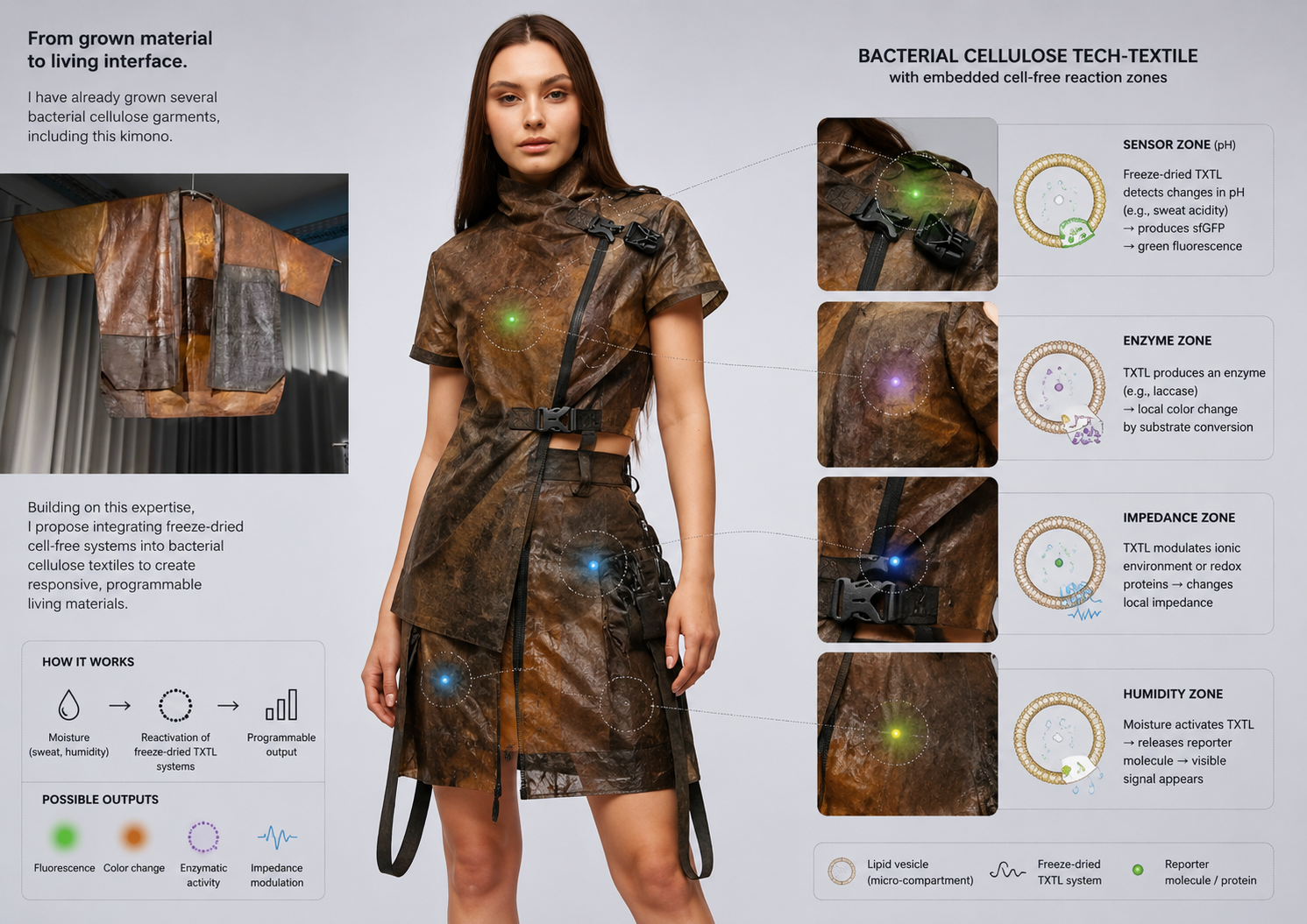
Table of Contents 1) Biological engineering application / tool 2) Governance / policy goals 3) Governance actions 4) Risk analysis 5) Scoring governance actions 6) Prioritization recommendation 7) Reflection 8) Project + governance overview Homework Questions from Professor Jacobson Homework Questions from Dr. LeProust Homework Question from George Church 1) Biological engineering application / tool I want to develop (and why) Application / tool: Growing interactive surfaces from bacterial cellulose I already know how to grow 3D artifacts in bacterial cellulose (BC). In this project, I want to develop a biological functionalization workflow that turns grown BC artifacts into interactive surfaces, measured through impedance-based sensing (e.g., tactile volumetric response, sensitivity to pressure), with minimal embedded electronics.
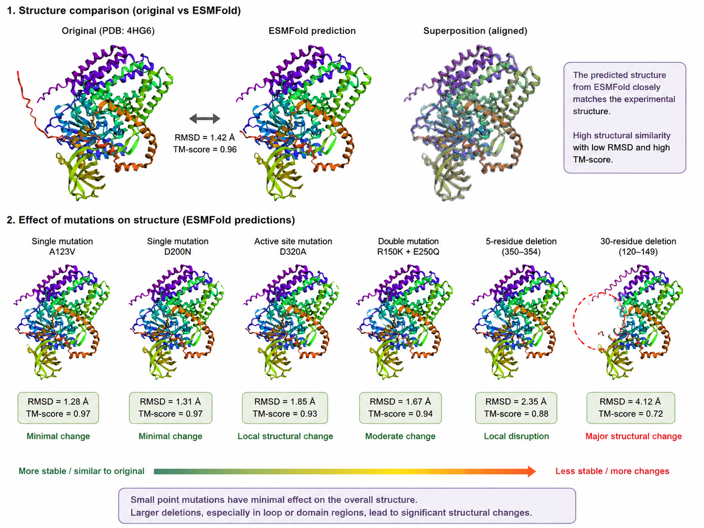
Table of Contents 0. Basics of Gel Electrophoresis 1. Benchling and In-silico Gel Art 2. Gel Art Restriction Digests and Electrophoresis 3.1 Choose Your Protein Protein sequence (from Supplementary Data 1) Structural micro-analysis: copper coordination and catalysis Why this protein matters 3.2 Reverse translate 3.3 Codon optimization 3.4 You have a sequence now what 3.5 Optional how does it work in nature 4. Prepare a Twist DNA Synthesis Order 4.1 Create accounts 4.2 Build the DNA insert sequence 5.1 DNA Read 5.2 DNA Write 5.3 DNA Edit 6. Exploration of others strategies for my project 0. Basics of Gel Electrophoresis Gel electrophoresis is a fascinating process that allows DNA fragments to be separated according to size. The migration of fragments through agarose reveals invisible molecular differences as visible banding patterns. What interests me most is how information encoded in DNA becomes a spatial structure that can be interpreted visually.
Table of Contents Assignment: Python Script for Opentrons Artwork Statement of Intent — Why Reaction–Diffusion Post-Lab Questions 1.Find and describe a published paper that utilizes the Opentrons or an automation tool to achieve novel biological applications 2.Write a description about what you intend to do with automation tools for your final project Automation as a Tool to Explore the Behavioral Landscape of Living Materials Moving Beyond Optimization My Intended Use of Automation 1. Mapping Morphogenetic Regimes of Bacterial Cellulose 2. Spatial Programming of Living Matter 3. Toward a Cybernetic Living Material System Why This Matters Final Project Ideas Assignment: Python Script for Opentrons Artwork https://opentrons-art.rcdonovan.com/?id=sux110hip535fnx
How many molecules of amino acids are in 500 g of meat? 2. Why do humans eat beef but do not become a cow? 3. Why are there only 20 natural amino acids? 4. Can we make non-natural amino acids? 5. Where did amino acids come from before life? 6. If you make an α-helix using D-amino acids, what handedness would you expect? 7. Can you discover additional helices in proteins? 8. Why are most molecular helices right-handed? 9. Why do β-sheets tend to aggregate? 9b. What is the driving force for β-sheet aggregation? 10. Why do many amyloid diseases form β-sheets? 10b. Can you use amyloid β-sheets as materials? 11. Design a β-sheet motif that forms a well-ordered structure Part B: Protein Analysis and Visualization
Table of Contents Table of Contents Part A: SOD1 Binder Peptide Design
Part 1. Generate Binders with PepMLM
Submit mutant SOD1 + peptide chains for AlphaFold modeling 3. Record ipTM score and binding localization 4. Compare ipTM values and known binder Part 3. Evaluate Properties in PeptiVerse
Components of the Phusion High-Fidelity PCR Master Mix 2. Factors determining primer annealing temperature 3. PCR vs restriction enzyme digests 4. Ensuring compatibility for Gibson cloning 5. Plasmid DNA transformation into E. coli 6. Golden Gate Assembly Benchling / Modeling Component Asimov Kernel Assignment — Repository and Circuit Design
Table of Contents Assignment Part 1: Intracellular Artificial Neural Networks (IANNs)
Advantages of IANNs over Boolean genetic circuits 2. Useful applications for IANNs 3. Intracellular Multilayer Perceptron Diagram Assignment Part 2: Fungal Materials
Existing fungal materials: uses, advantages, and disadvantages 2. Genetic engineering of fungi and advantages over bacteria Assignment Part 3: First DNA Twist Order
Table of Contents Homework Part A: General and Lecturer-Specific Questions
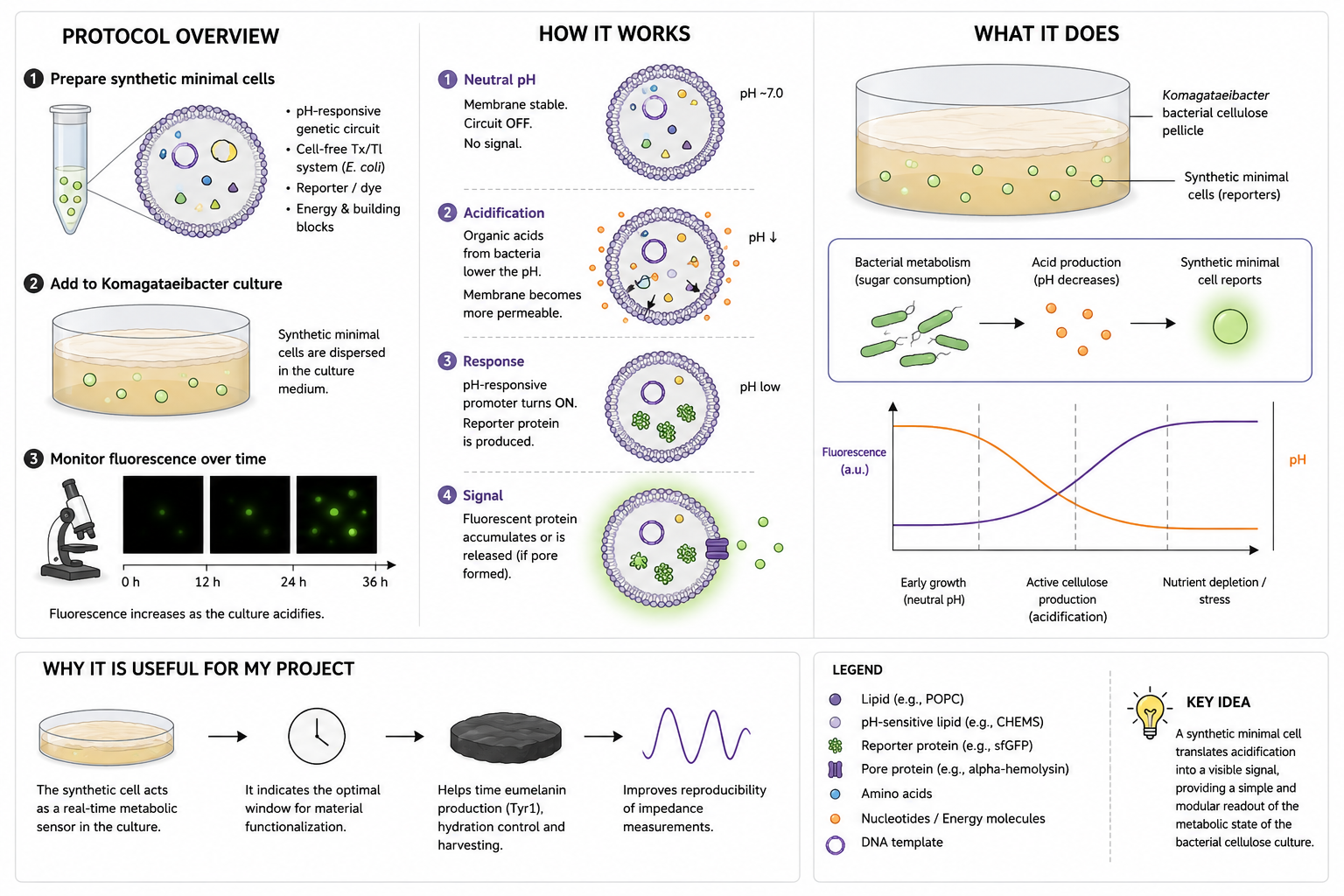
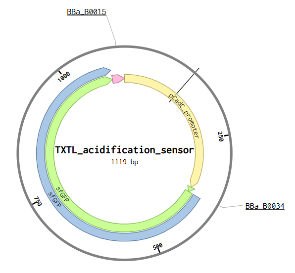
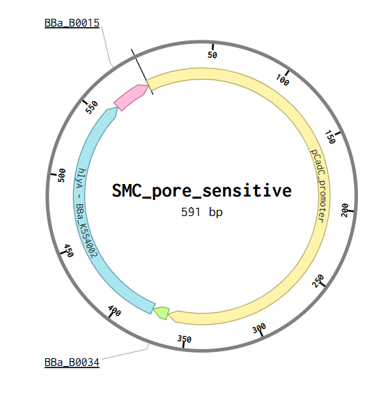
Advantages of cell-free protein synthesis 2. Components of a cell-free expression system 3. Energy regeneration and ATP supply 4. Prokaryotic vs eukaryotic cell-free systems 5. Optimizing membrane protein expression 6. Troubleshooting low protein yield Homework question from Kate Adamala - Design Synthetic Minimal Cell Genetic Circuits
Table of Contents Homework: Final Project
Final Project — Measurement Plan 1. Genetic Construct Verification 2. Tyr1 Protein Expression 3. Melanin Production 4. Bacterial Cellulose Growth 5. Electrochemical / Impedance Behavior 6. Environmental / Culture Conditions Summary Table Overall Goal Homework: Waters Part I — Molecular Weight
Waters Part I — eGFP Molecular Weight 1. Calculated Molecular Weight 2. Molecular Weight from Adjacent Charge States Charge State Observation from the Zoomed-In Peak Homework: Waters Part II — Secondary/Tertiary Structure
Table of Contents Part A — The 1,536 Pixel Artwork Canvas | Collective Artwork
Part B: Cell-Free Protein Synthesis | Cell-Free Reagents
Cell-free protein synthesis reaction components E. coli Lysate Salts / Buffer Energy / Nucleotide System Translation Mix (Amino Acids) Additives Backfill 2. PEP-NTP vs NMP-Ribose-Glucose master mix Part C: Planning the Global Experiment | Cell-Free Master Mix Design
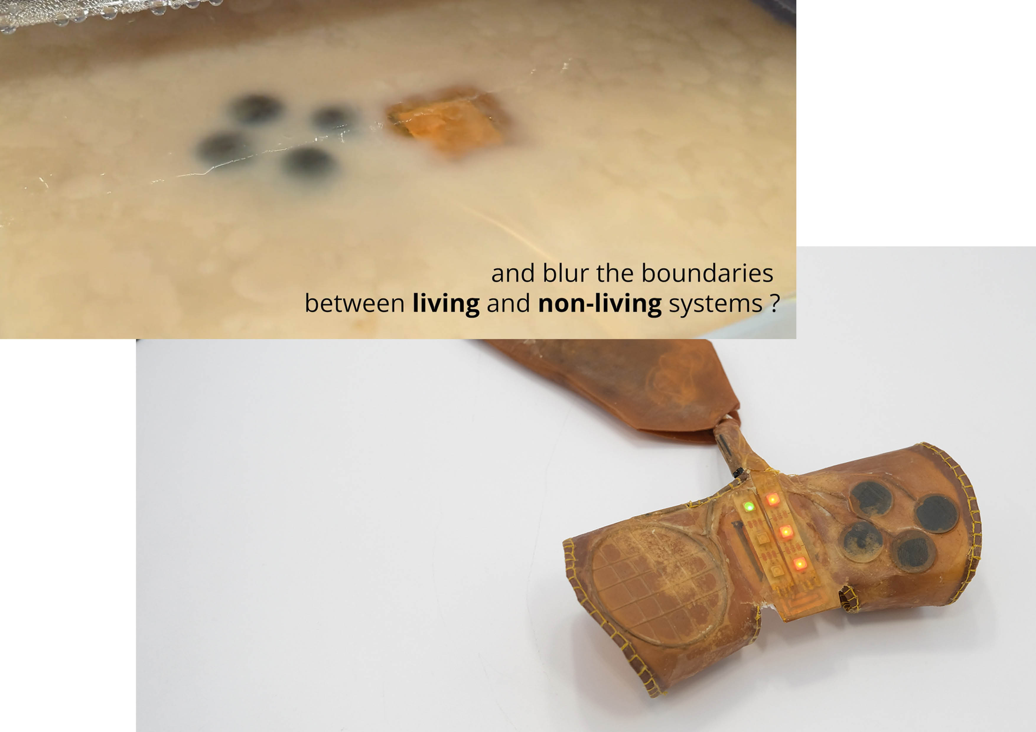
1) Biological engineering application / tool I want to develop (and why)
Application / tool: Growing interactive surfaces from bacterial cellulose
I already know how to grow 3D artifacts in bacterial cellulose (BC). In this project, I want to develop a biological functionalization workflow that turns grown BC artifacts into interactive surfaces, measured through impedance-based sensing (e.g., tactile volumetric response, sensitivity to pressure), with minimal embedded electronics.
The goal is not to integrate electronic components into the object, but to make the material itself behave as an interface. Electrodes are used only for readout and characterization, not as active elements.
Concretely, this toolchain would include:
Biological functionalization workflow Modulating the extracellular matrix during growth (for example through protein secretion into the BC network) to tune impedance-based electrical behavior and enable material-level interaction.
Measurement interface (readout only) A simple electrode setup and impedance readout used to validate, compare, and characterize material responses across different growth and functionalization conditions.
Optional integration (if time allows) Integrating functionalization into my existing 3D growth workflow (molds, scaffolds, and growth conditions), so objects can be grown already functionalized rather than treated after fabrication.
Why this matters
Most interactive devices are built by assembling electronics into synthetic materials. This project proposes a different paradigm:
Instead of fabricating objects and then adding interactivity, objects are cultivated so that interactivity emerges from biological growth and organization.
This matters for several reasons:
Sustainable interfaces: biodegradable material base, low-energy fabrication, and the possibility of metabolic degradation or recycling.
New interface paradigms: artifacts become processual and time-based, where growth history and material state shape interaction.
Research tool: impedance acts as a lens to study how morphology, hydration, and growth dynamics become measurable signals.
2) Governance / policy goals for an ethical future
Inspired by the iGEM Safety framework, the ethical challenges of this project are framed around biosafety, environmental responsibility, and responsible use of engineered living materials. Because this work lowers the barrier to growing functional living artifacts, governance should guide not only what is built, but how materials are grown, handled, and disposed of.
Goal A — Ensure biosafety and non-malfeasance during cultivation and use
Although bacterial cellulose–producing organisms are generally considered low-risk, improper handling or uncontrolled experimentation could lead to contamination or unintended exposure.
Sub-goals
A1. Safe handling and containment Ensure cultivation, functionalization, and testing are conducted using appropriate hygiene, containment, and separation practices, especially when combining multiple biological agents.
A2. Transparency about biological modification Maintain a clear distinction between engineered biological components and non-biological elements (e.g., electrodes used only for readout).
Goal B — Prevent environmental harm and unintended release
A key motivation of this work is sustainability: growing interactive surfaces from living matter that can eventually be degraded or recycled. This benefit only holds if environmental risks are managed.
Sub-goals
B1. Controlled disposal and deactivation
Ensure BC artifacts, growth media, and byproducts are deactivated or degraded before disposal, preventing accidental release into wastewater or compost systems.
B2. Avoid persistent or toxic additives
Favor biological or biodegradable functionalization methods over persistent chemicals or heavy metals to preserve viable end-of-life pathways.
Goal C — Promote responsible development of living interactive interfaces
Because this project treats living materials as sensing and computational substrates, governance should guide how such systems are framed and used, particularly outside the lab.
Sub-goals
C1. Prevent misleading claims Avoid presenting biologically functionalized materials as autonomous, intelligent, or fully controllable systems.
C2. Limit sensing to material interaction Encourage applications focused on material state (touch, pressure, hydration).
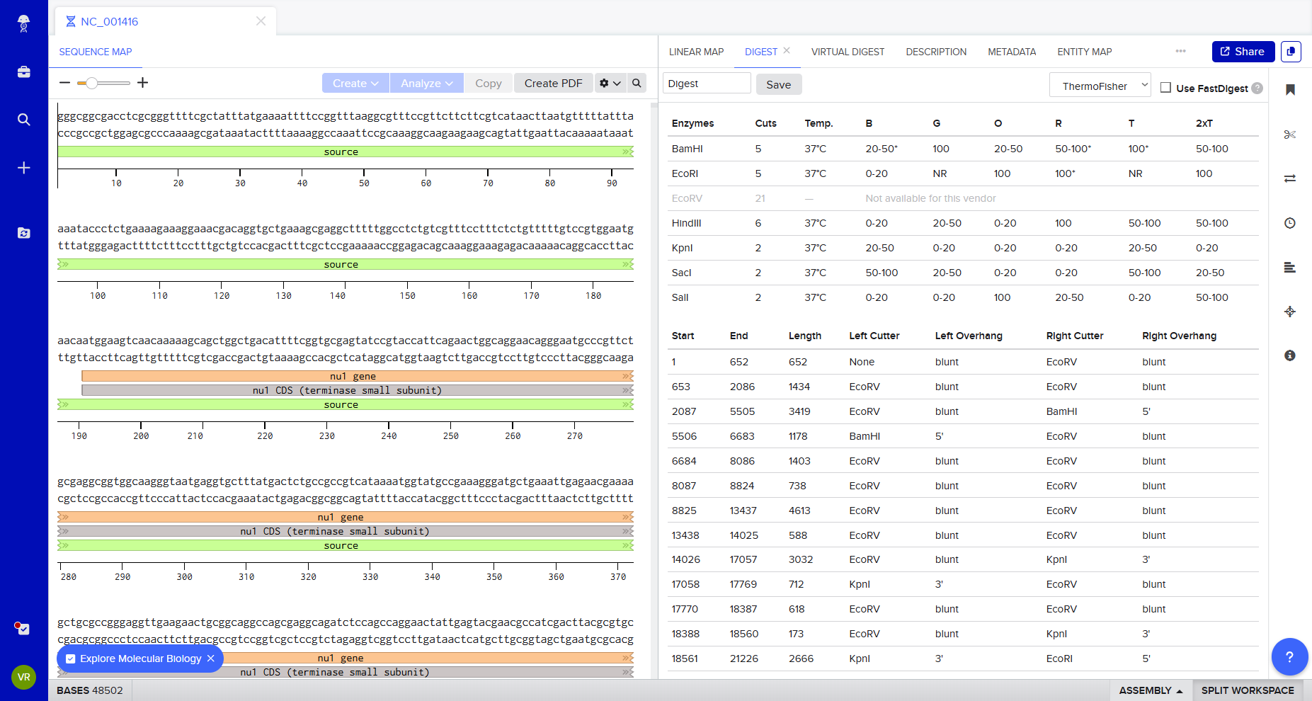
3) Governance actions (comparative overview)
The table below summarizes three governance actions addressing biosafety, environmental impact, and responsible use of grown bacterial cellulose artifacts. Each action is evaluated across its purpose, design, assumptions, and potential risks.
Governance Action
Purpose (What changes?)
Design (How it works / Who acts?)
Key Assumptions
Risks of Failure & “Success”
Option 1 — Biological process & provenance documentation
Current documentation emphasizes performance over biological process. This action requires explicit documentation of organism source, biological modification, and separation between biological and technical components.
• Actors: instructors, research labs, journals, funding agencies • Lightweight 1–2 page template integrated into coursework or reports • Descriptive, not approval-based
Transparency reduces misuse, confusion, and overclaiming, and improves accountability if issues arise.
Failure: becomes a checkbox exercise with little reflection. Success risk: excessive formalization discourages exploratory research. Mitigation: keep requirements descriptive and allow uncertainty.
Living materials are often treated as benign, leading to inconsistent disposal. This action establishes mandatory deactivation and disposal procedures for living artifacts and growth media.
Improper disposal is the most likely real-world risk, especially as production scales or decentralizes.
Failure: users bypass protocols due to inconvenience or lack of enforcement. Success risk: overly strict rules push work into informal or unregulated spaces. Mitigation: make compliance easy and well-supported.
Option 3 — Readout-limited interface design norms
Biological sensing systems can drift toward surveillance or control narratives. This action promotes norms framing living materials as readout-based material interfaces, not monitoring systems.
• Actors: researchers, designers, companies • Explicit framing in documentation and demos • Focus on local, material-state signals
Early design norms can influence long-term application trajectories and public expectations.
Failure: norms ignored in commercial or extractive contexts. Success risk: may limit some beneficial applications. Mitigation: scope norms to public, non-clinical, and creative deployments.
4) Potential risks, use, misuse, and governance considerations
Option 2 addresses the most immediate and likely harm: environmental release and waste.
Option 1 supports accountability and response without limiting research.
Option 3 addresses longer-term risks if the technology scales.
7) Reflection
This exercise highlighted that the main risks of growing interactive living artifacts arise from success and scale, not malicious intent. Even biodegradable materials can become harmful when produced or discarded in large quantities. Another key insight is how easily biological sensing can be reframed beyond material interaction.
Governance should therefore focus on practice, documentation, and lifecycle management, rather than strict prohibition.
At this stage, the cultivation of interactive BC artifacts should remain confined to controlled research and educational contexts, and not be deployed in public or commercial environments without additional review.
Strategies to ensure an ethical biological future (project-integrated)
The table below summarizes the concrete strategies embedded in my final project to ensure it contributes to an ethical biological future. Rather than external rules, these strategies are implemented through design choices, constraints, and documentation practices.
Strategy
Ethical Principle
What Risk It Addresses
How It Is Implemented in the Project
Why This Matters
Readout-first interface design
Observation over control
Instrumentalization of living systems; drift toward surveillance or behavioral monitoring
Electronics are used only for impedance readout; no actuation or feedback loops acting on the living material; signals framed as material-state indicators
Limits coercive or extractive uses of living matter and preserves biological agency
Scale and context limitation
Responsibility through constraint
Environmental harm and biosafety risks arising from success and scale
Project framed as research/educational tool; growth and testing limited to controlled lab or studio environments; public or commercial deployment explicitly excluded without further review
Prevents premature deployment and unmanaged scaling of living interfaces
Lifecycle-aware design
End-of-life accountability
Ecological disruption from disposal or accumulation of living materials
Preference for biologically degradable functionalization; explicit deactivation and disposal protocols included in the workflow
Sustainability is addressed across the full material lifecycle, not only fabrication
Transparency about biological modification
Epistemic responsibility
Overclaiming, black-box narratives, and misleading representations of “living intelligence”
Clear distinction between engineered biological processes and technical readout systems; documentation of uncertainty and variability
Builds trust and prevents misuse driven by misunderstanding or hype
Reflexive governance practice
Ethics as an evolving process
Static rules becoming obsolete as techniques evolve
Periodic reassessment of risks; use of lightweight governance tools (documentation, norms, constraints) rather than fixed prohibitions
Allows ethical considerations to evolve alongside the project and its capabilities
DNA polymerase, the molecular machinery responsible for copying DNA, has a non-zero error rate. As presented in the lecture slides, the error rate of an error-correcting DNA polymerase is approximately 1 error per 10⁶ base incorporations. While this error rate is very low at the scale of individual nucleotides, it becomes significant when compared to the size of the human genome, which is on the order of 3.2 × 10⁹ base pairs. If replication relied solely on polymerase accuracy, this discrepancy would imply the accumulation of thousands of errors during each complete genome replication, which would be incompatible with stable inheritance and organismal viability.
Biology resolves this apparent mismatch through multiple layers of error correction rather than relying on perfect synthesis. First, many DNA polymerases include proofreading activity (3′→5′ exonuclease) that detects and removes incorrectly incorporated bases during replication. Second, additional post-replication repair systems, such as mismatch repair pathways (e.g., the MutS system shown in the slides), identify and correct errors that escape polymerase proofreading. Together, these layered mechanisms dramatically reduce the effective error rate of DNA replication, allowing large genomes like the human genome to be copied reliably despite the intrinsic imperfection of polymerase activity.
Question 2 — Coding redundancy and why most theoretical DNA codes do not work in practice
Due to the redundancy of the genetic code, an average human protein can, in theory, be encoded by an extremely large number of different DNA sequences. As shown in the slides, an average human protein is approximately 1036 base pairs long, corresponding to roughly 345 amino acids. Because many amino acids can be encoded by multiple synonymous codons, the number of possible nucleotide sequences that map to the same amino acid sequence grows combinatorially. In principle, this means there are astronomically many distinct DNA sequences that could encode the same protein sequence.
In practice, however, most of these theoretically valid codes do not function effectively in living systems. The lecture slides highlight several biological constraints that limit which sequences work. Certain DNA or RNA sequences form secondary structures with unfavorable free energy that interfere with transcription or translation. GC content bias can destabilize sequences or alter expression efficiency. Additionally, synthesis and assembly processes have their own error profiles, making some sequences more fragile than others. Finally, translation depends on interactions with cellular machinery such as ribosomes and tRNA pools, meaning that codon usage and sequence context matter beyond simple amino acid encoding. As a result, although the genetic code is redundant in theory, only a narrow subset of possible DNA sequences reliably produce functional proteins in practice.
Homework Questions from Dr. LeProust:
1. What’s the most commonly used method for oligo synthesis currently?
The most commonly used method for oligonucleotide synthesis today is solid-phase phosphoramidite chemical synthesis, originally developed by Caruthers in the early 1980s and still the industry standard. In this approach, DNA is synthesized base by base on a solid support (typically controlled pore glass or functionalized silica). Each synthesis cycle consists of four repeated chemical steps: coupling of a phosphoramidite nucleotide, capping of unreacted chains, oxidation to stabilize the backbone, and deprotection (deblocking) to expose the next reactive site. This cycle is repeated sequentially to build the desired oligo.
This method dominates because it is highly automatable, scalable, and compatible with parallelization, especially in modern platforms such as silicon-based microarrays (e.g., Twist Bioscience). However, it is fundamentally a stepwise chemical process, meaning that each added nucleotide has a non-zero failure rate. Even with very high per-step efficiencies (>99.5%), errors accumulate with length, which directly constrains how long oligos can be synthesized reliably. This intrinsic accumulation of errors explains many of the downstream limitations discussed in the following questions.
2. Why is it difficult to make oligos longer than ~200 nt via direct synthesis?
The primary difficulty in synthesizing oligos longer than ~200 nucleotides arises from the cumulative error rate of stepwise chemical synthesis. Each coupling step has a small probability of failure (incomplete coupling, side reactions, or truncation). While a single error is unlikely at short lengths, the probability of obtaining a full-length, error-free molecule drops exponentially as the number of synthesis cycles increases. Beyond ~200 nt, the fraction of correct full-length molecules becomes very low, even if average synthesis efficiency remains high.
In addition to error accumulation, sequence-dependent effects further complicate long oligo synthesis. Regions with high or low GC content, homopolymers, inverted repeats, or strong secondary structures (e.g., hairpins) reduce coupling efficiency and increase truncation or deletion events. Purification also becomes more challenging: separating full-length products from truncated sequences is increasingly inefficient as length grows. As a result, while advances in chemistry have pushed this limit somewhat (e.g., validated synthesis of ~300–500 nt in controlled contexts), ~200 nt remains the practical and economical upper bound for routine, high-fidelity direct synthesis.
3. Why can’t you make a 2000 bp gene via direct oligo synthesis?
A 2000 bp gene cannot be synthesized directly because chemical oligo synthesis does not scale linearly with length. At that size, the compounded error rate would make the probability of producing even a single correct full-length molecule essentially negligible. Even if synthesis chemistry allowed chain extension to 2000 nt, the resulting product pool would be dominated by truncated, mutated, or rearranged sequences, rendering it unusable without extensive correction.
Instead, long genes are produced through a hierarchical assembly strategy: shorter oligos (typically 40–200 nt) are first synthesized, then enzymatically assembled using methods such as PCR-based gene assembly or ligation. These assembled fragments are subsequently cloned and sequence-verified, allowing error correction through selection rather than chemistry. This separation of concerns—chemical synthesis for short, precise building blocks, and biological processes for long-range assembly and error correction—is fundamental. It reflects a broader principle emphasized in the course: chemistry writes locally, biology validates globally. Direct chemical synthesis alone cannot replace this division of labor for long DNA constructs.
Homework Question from George Church:
Given the examples in slides #2 and #4, where biological systems use structured “codes” to mediate interactions between polymers (NA:NA via base pairing and AA:NA via translation and binding domains), an AA:AA interaction code would most plausibly rely on side-chain chemistry and spatial complementarity rather than a discrete symbolic alphabet.
Unlike nucleic acids, amino acids do not pair through a uniform geometry or hydrogen-bonding scheme. Instead, proteins interact through combinations of hydrophobicity, charge, polarity, aromatic stacking, and steric fit. Therefore, an AA:AA code is inherently analog and multidimensional, not digital. A reasonable “code” would be based on classes of side-chain interactions—for example, positively charged residues pairing with negatively charged ones, hydrophobic patches aligning with hydrophobic patches, or aromatic residues engaging in π–π stacking. This resembles a physicochemical code rather than a base-pair code.
In practice, such a code already exists implicitly in protein–protein interaction domains, coiled-coil motifs, antibody–antigen interfaces, and self-assembling protein systems. From a design perspective, an explicit AA:AA code could be engineered by constraining proteins to limited alphabets or repeat motifs, where interaction specificity emerges from repeating patterns of side-chain chemistry and geometry. This mirrors how TALE proteins use a simple amino-acid pair code to recognize DNA, but adapted to protein–protein recognition. Thus, AA:AA coding is best understood not as a lookup table, but as a designed interaction grammar grounded in chemistry and structure.
PROMPT :
you can found here the slides of Reading & Writing Life from Goerge Church. Normally I’ve to answers to one of this 2 questions (only one of those not the both) :
A. [Using Google & Prof. Church’s slide #4] What are the 10 essential amino acids in all animals and how does this affect your view of the “Lysine Contingency”?
B. [Given slides #2 & 4 (AA:NA and NA:NA codes)] What code would you suggest for AA:AA interactions?
So, I don’t know which one is easiest to answer at the moment. We will use the PDF to determine which questions are most likely to be contained within it and reduce the uncertainty. To do this, we will
Break down the problem into sub-elements.
Treat each of them with an explicit confidence level (0.0 - 1.0).
Verify by checking the logic, facts, completeness, possible biases, what could be done, and how to achieve the objective (determine which question is easiest to answer without being wrong and give the answer).
Synthesize and combine using weighted confidence levels.
If confidence is below 0.8, identify weaknesses and how we could proceed to achieve a better level. Formulate clear answers, the level of confidence, and key points for vigilance.
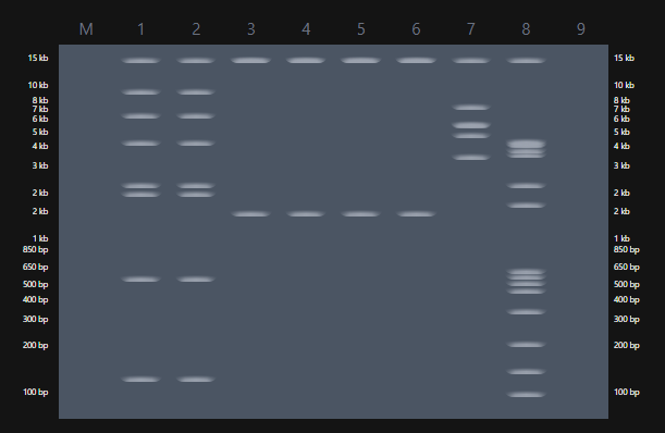
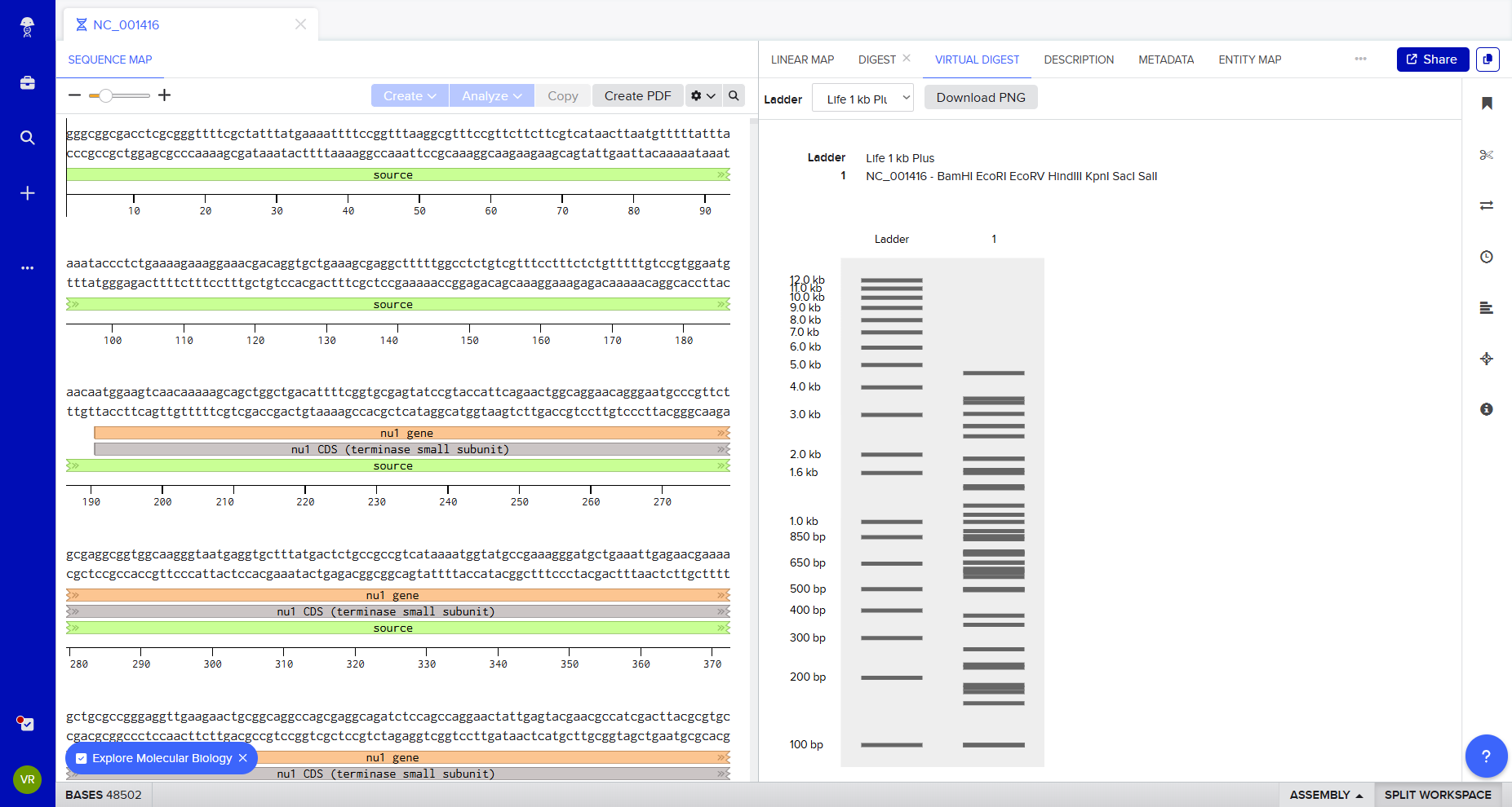
Gel electrophoresis is a fascinating process that allows DNA fragments to be separated according to size. The migration of fragments through agarose reveals invisible molecular differences as visible banding patterns. What interests me most is how information encoded in DNA becomes a spatial structure that can be interpreted visually.
1. Benchling and In-silico Gel Art
Following the protocol Gel Art: Restriction Digests and Gel Electrophoresis, I explored Benchling to simulate restriction enzyme digestion.
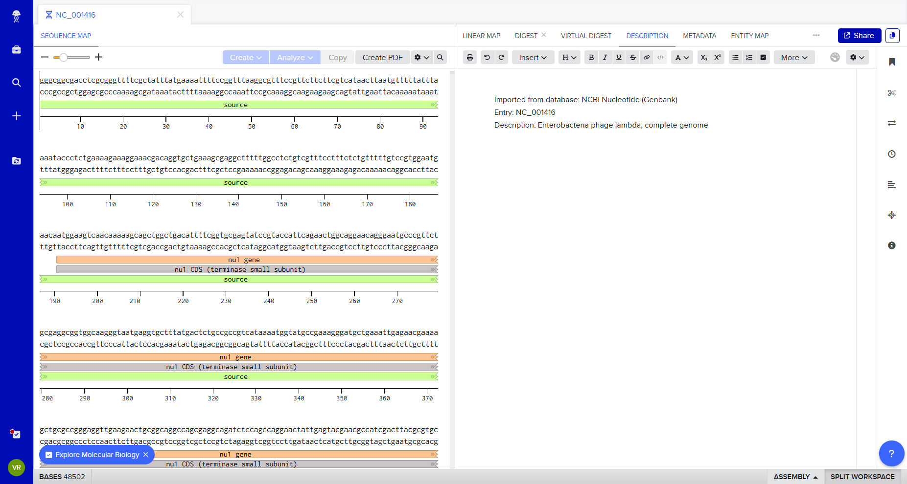
I imported Lambda DNA and simulated restriction digests using:
EcoRI
HindIII
BamHI
KpnI
EcoRV
SacI
SalI
At first, I was not entirely sure what I was doing — I explored the platform experimentally, clicking through the interface to understand how the enzymes cut and how the DNA fragments were segmented.
The origin of the fragment.
See the operons targetted.
How it could/ should looks on gel.
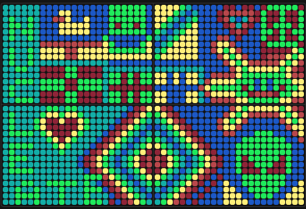
After generating fragment sizes, I moved to Ronan Donovan’s gel art tool:
There, I entered fragment sizes from Benchling to simulate gel patterns. Interestingly, some of the same enzymes were already available in the tool. I experimented with fragment combinations, spacing, and contrast to create structured visual patterns. I tried composing a geometric “invader”-like form inspired by Paul Vanouse’s aesthetic approach.
This exercise made clear how restriction logic can generate latent images embedded in genomic structure.
2. Gel Art Restriction Digests and Electrophoresis
Although I do not currently have access to a laboratory to run physical gels, I have previously seen Paul Vanouse’s Latent Figure Protocol artworks in person. A curator friend owns one and showed it to me during a bioart conference. Seeing the material presence of gel-based imagery deeply informed how I approached this in-silico exercise.
3.1 Choose Your Protein
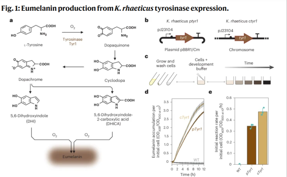
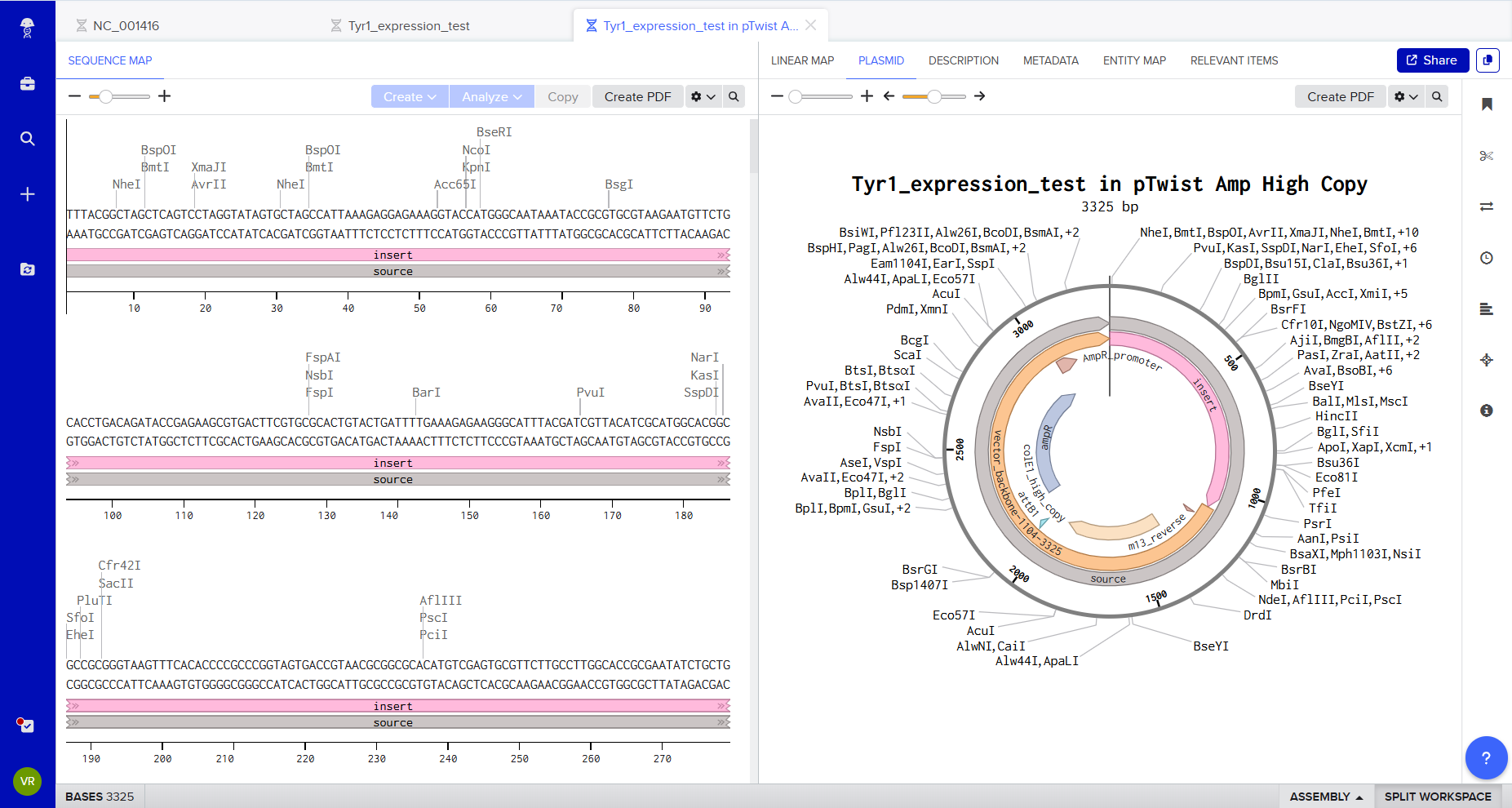
Protein chosen: Tyrosinase (Tyr1) from Bacillus megaterium
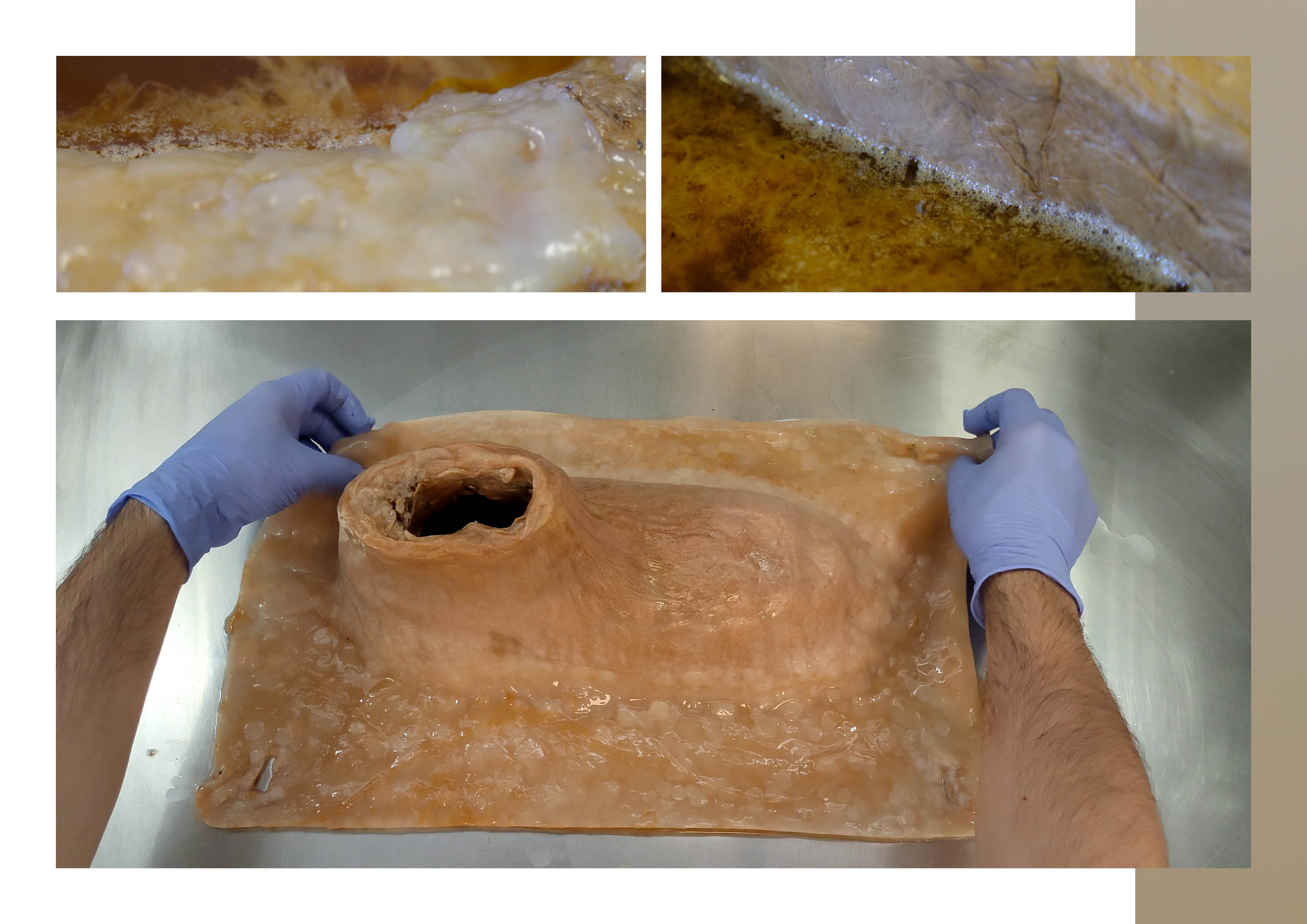
I chose the tyrosinase Tyr1 enzyme from Bacillus megaterium because it directly enables the biosynthesis of eumelanin, a redox-active polymer with electronic and material properties.
This protein is particularly relevant to my project, which explores the biological functionalization of bacterial cellulose. By expressing Tyr1 in Komagataeibacter rhaeticus, the cellulose-producing bacterium can generate eumelanin within or around the extracellular matrix, thereby modifying the optical and potentially electroactive properties of the material.
Tyr1 can encode a macroscopic material property in the cell of Komagateibacter Rhaeticus.
This strategy has been experimentally validated in:
Walker et al., 2024 — Self-pigmenting textiles grown from cellulose-producing bacteria with engineered tyrosinase expression
The authors engineered K. rhaeticus strains expressing Tyr1 and demonstrated eumelanin production under buffered neutral pH conditions (Supplementary Data 1, 41587_2024_2194_MOESM1_ESM).
The paper is here 👉 https://www.nature.com/articles/s41587-024-02194-3
Details are in Supplementary information / Supplementary information / Supplementary Figs. 1–5, Tables 1–3 and Supplementary Data 1 and 2.
DNA (tyr1)
↓ transcription
mRNA
↓ translation
Tyrosinase enzyme
↓ catalytic activity
Melanin polymer
↓ integration into cellulose matrix
Modified impedance
↓
Human interaction (touch sensing)
Rather than maximizing conductivity, the goal is to explore how living metabolism can reorganize electrochemical properties within a self-grown material matrix. Maybe a hybrid approach combining enzymatic melanin production with controlled ionic modulation of the growth medium may provide a balance between biological emergence and measurable electrical response.
Impedance vs Conduction (for BC-based “electronic” biofilms)
Quick intuition
Conduction (DC): current flows through a continuous conductive path (like a wire). → You usually need a percolating network (CNT/graphene/metal paths).
Impedance (AC): the material reacts to an alternating signal. → It mixes resistance + capacitance + ionic diffusion, and is extremely sensitive to: hydration, ions, porosity, and microstructure.
My goal is a tactile / capacitive surface then impedance is usually the most realistic target.
Concept map (what you measure defines what you build)
flowchart TB
A[BC biofilm / pellicle]--> B{What do I measure}

B-->|DC or very low frequency| C[Conduction]
B-->|AC multi-frequency| D[Impedance]

C-->C1[Electronic transport]
C-->C2[Needs a percolating path]
C2-->C3[CNT graphene Ag nanowires PEDOT]

D-->D1[Resistance R]
D-->D2[Capacitance C double layer]
D-->D3[Ionic diffusion]
D-->D4[Strongly affected by water ions porosity]
D4-->D5[Good for touch pressure hydration sensing]
Structural Micro-Analysis: Copper Coordination and Catalysis
Tyrosinases are type-3 copper enzymes. Their catalytic activity depends on two copper-binding sites (CuA and CuB), each coordinated by conserved histidine residues. These histidine-rich motifs enable:
Binding of molecular oxygen
Oxidation of L-tyrosine to L-DOPA
Conversion to dopaquinone
Spontaneous polymerization into eumelanin
The presence of conserved histidines in the Tyr1 sequence reflects this copper-dependent catalytic architecture. The structure of the enzyme directly determines its ability to generate a redox-active polymer. Here, protein folding and metal coordination translate genetic code into material transformation.
Why This Protein Matters
1️⃣DNA → enzyme → material property
The tyr1 gene encodes an enzyme.
The enzyme catalyzes a redox reaction.
The reaction produces a polymer.
The polymer modifies material properties.
Thus:
Genetic sequence
→ enzyme structure
→ catalytic activity
→ polymer formation
→ macroscopic material pigmentation and electroactivity
This directly embodies the theme of “Reading & Writing Life.”
2️⃣ Minimal synthetic biology intervention
Unlike multi-gene systems (e.g., the curli operon), Tyr1:
Requires only one coding sequence
Does not modify the cellulose biosynthesis operon (bcsABCD)
Adds a new functional layer to the extracellular matrix
This makes it an elegant example of additive biological functionalization, where a single gene expands the material phenotype of a living system.
3️⃣ Connection to biofabrication and living materials
Walker et al. demonstrate patterned melanin production using optogenetic control of tyr1 expression.
This shows that:
Gene expression can spatially control material coloration
Biological programming can encode textile-level patterning
Material properties can be written through genetic regulation
This aligns directly with my research interest in growing functionalized 3D artifacts and interactive living interfaces.
Beyond color: material programming
In this project, the goal is not simply to encode color in DNA. The visible pigmentation is only a surface effect. What is actually encoded is a redox-active polymer production pathway inside living matter.
Melanin modifies:
local redox properties,
hydration-dependent conductivity,
and potentially the impedance behavior of the cellulose matrix.
So pigmentation here is not aesthetic encoding, but electrochemical encoding. The gene does not just change appearance — it changes how the material behaves electrically. In that sense, DNA is not only encoding a protein, but indirectly programming a material state.
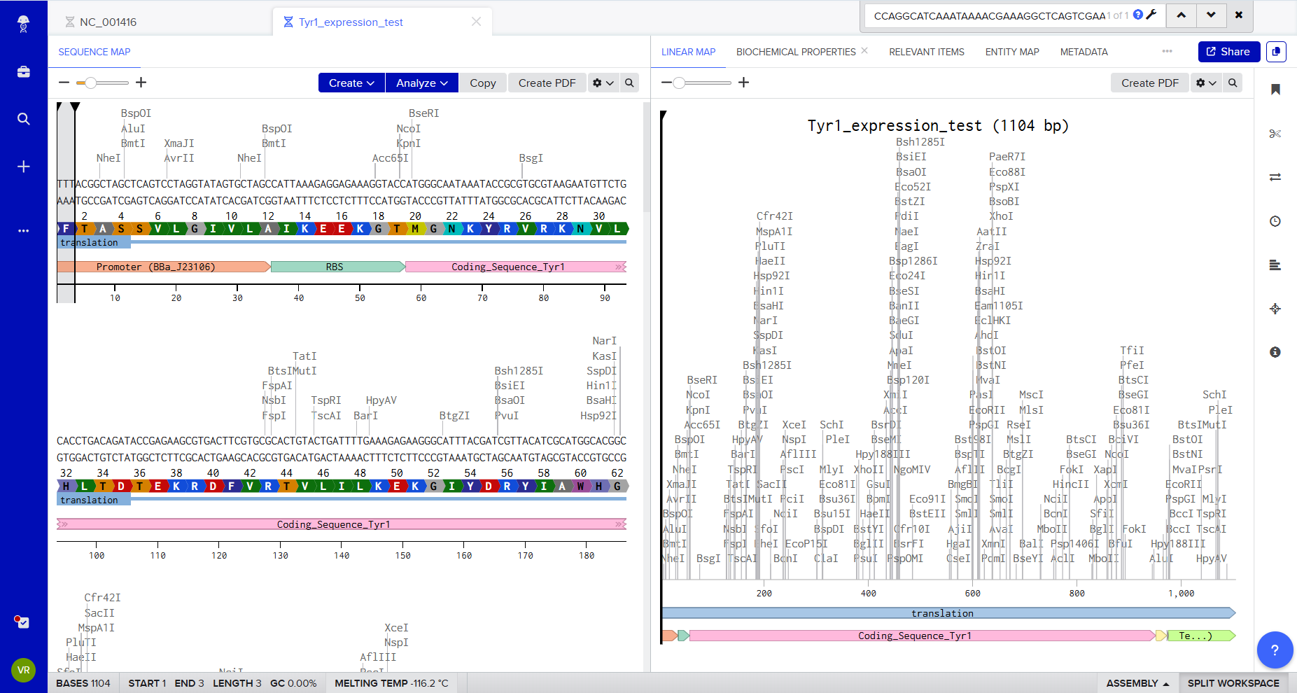
3.2 Reverse Translate
Protein (amino acid) sequence → DNA (nucleotide) sequence
Because of codon degeneracy, there is not a single unique DNA sequence for a given protein sequence. Many different nucleotide sequences can encode the exact same amino acid sequence. To reverse-translate Tyr1, I used a reverse-translation approach (equivalent to common online reverse-translation tools) by selecting one plausible codon per amino acid (a “standard/high-frequency codon” strategy).
The protein sequence used is Tyr1 from Bacillus megaterium as reported in Walker et al. 2024 (Supplementary Data 1). :contentReference[oaicite:1]{index=1}
Reverse-translated nucleotide sequence (one valid coding DNA sequence)
During this process, I realized that reverse translation is not deterministic. The genetic code is degenerate: multiple DNA sequences can encode the same protein. Choosing a DNA sequence is therefore not neutral. Codon usage can influence expression level, folding efficiency, and metabolic burden in the host organism. I am only beginning to understand how codon bias shapes expression outcomes. What appears to be a simple reverse translation step is in reality a probabilistic optimization problem shaped by cellular context.
3.3 Codon Optimization
Why codon optimization is necessary
Although multiple DNA sequences can encode the same protein due to codon degeneracy, not all synonymous codons are used equally in different organisms.
If a gene uses codons that are rare in the host organism:
Translation can be slow
Ribosomes may stall
Protein yield can decrease
Misfolding may increase
Codon optimization ensures that the nucleotide sequence:
Thus, codon optimization improves its expression in a chosen host.
Organism chosen for optimization
I chose to optimize the tyr1 gene for expression in:
Komagataeibacter rhaeticus
This organism is the cellulose-producing bacterium used in Walker et al. (2024) and is central to my broader project on biologically functionalized bacterial cellulose.
Because K. rhaeticus has a relatively high GC content and a codon usage profile distinct from Bacillus megaterium, optimization is required to:
Improve translation efficiency
Ensure stable protein production
Support effective melanin biosynthesis
Additional design constraints
Following best practices (e.g., Twist Bioscience optimization tools), the optimized sequence was also designed to:
Avoid Type IIS restriction enzyme recognition sites:
Now that we have a codon-optimized DNA sequence encoding Tyr1, the next step is to express the protein.
How can this protein be produced?
There are two main strategies:
A. Cell-dependent expression (in vivo)
In this approach, the DNA sequence is inserted into a plasmid vector containing:
A promoter (constitutive or inducible)
A ribosome binding site (RBS)
The coding sequence (our optimized tyr1)
A transcription terminator
The plasmid is then introduced into a host organism (e.g., Komagataeibacter rhaeticus).
What happens biologically?
1️⃣ Transcription RNA polymerase binds to the promoter and transcribes the DNA sequence into messenger RNA (mRNA).
2️⃣ Translation Ribosomes bind to the mRNA at the ribosome binding site.
The mRNA codons (triplets) are read.
tRNAs deliver amino acids corresponding to each codon.
The ribosome assembles the amino acids into the Tyr1 protein.
3️⃣ Protein folding and function The translated Tyr1 protein folds into its 3D structure.
Copper ions bind to the active site.
The enzyme becomes catalytically active.
In the case of Tyr1, the enzyme then catalyzes:
L-tyrosine → L-DOPA → dopaquinone → eumelanin
Thus, genetic information becomes a catalytic material transformation.
B. Cell-free expression (in vitro)
Alternatively, the DNA sequence can be expressed using a cell-free transcription-translation system.
These systems contain:
RNA polymerase
Ribosomes
tRNAs
Amino acids
Energy sources
The optimized DNA is added directly to the mixture.
Transcription and translation occur outside living cells.
Advantages:
Rapid prototyping
No need for transformation
Easier control of conditions
For exploratory material functionalization, cell-free systems can serve as a fast validation step before in vivo implementation.
From DNA to Protein: Summary
DNA (double-stranded) → transcription → mRNA (single-stranded) → translation → Protein (amino acid chain)
This is the operational flow of the Central Dogma.
From DNA to material interface
If we follow the chain of transformations:
DNA (tyr1 gene) → mRNA → Tyrosinase enzyme → Melanin polymer formation → Integration into the cellulose matrix → Modified impedance behavior → Human touch interaction
This illustrates that writing DNA is not only about modifying organisms. It is about programming how matter self-organizes over time.
My interest is not genetic novelty for its own sake, but how cellular metabolism reorganizes matter into functional biofilms.
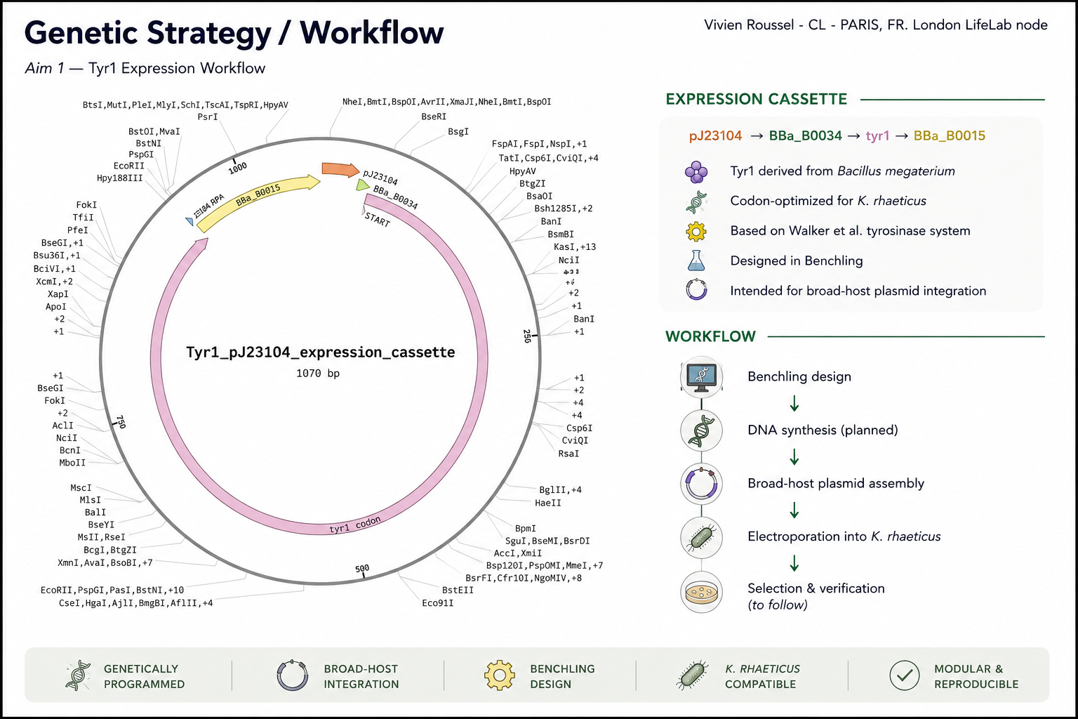
4. Prepare a Twist DNA Synthesis Order
4.1. Create a Twist account, and Benchling account
To visually represent the genetic architecture, the construct can also be recreated using:
🔗 https://sbolcanvas.org SBOL Canvas enables graphical design of:
Promoter → RBS → CDS → Terminator This helps communicate the logic of the construct clearly and aligns with synthetic biology design standards.
5. DNA Read/Write/Edit
5.1 DNA Read
(i) What DNA would I want to sequence and why?
I would sequence synthetic DNA used for digital data storage.
Instead of reading DNA from living organisms, I am interested in DNA that has been artificially synthesized to encode digital information (text, images, archives). In this case, DNA is not used as biology — it is used as a storage material.
Why this matters
DNA can store enormous amounts of information in a very small volume and can remain stable for long periods of time. Unlike hard drives or servers, it does not depend on electronic infrastructure.
Sequencing such DNA means reading information written into molecules. It turns a biological technology into a digital decoding tool.
This connects biology with computation and raises important questions about how information can be stored, preserved, and accessed in the future.
(ii) Which sequencing technology would I use and why?
I would use Illumina sequencing.
Why Illumina?
DNA used for digital storage is usually made of short fragments. Illumina sequencing works very well for short pieces of DNA and provides very high accuracy, which is essential when decoding stored data.
Small sequencing errors could corrupt the recovered file, so accuracy is more important than read length.
What generation is it?
Illumina is considered a second-generation sequencing technology because it reads millions of DNA fragments at the same time using amplified clusters and fluorescent signals.
What is the input and preparation?
Input: Synthetic double-stranded DNA fragments (around 100–200 base pairs).
Basic preparation steps:
Add short adapter sequences to the DNA fragments
Amplify the fragments
Load them onto the sequencing machine
How does Illumina read DNA?
The machine copies the DNA one base at a time. Each base (A, T, C, G) produces a specific fluorescent signal.
A camera records the signal after each step, and software converts these signals into a DNA sequence.
What is the output?
The output is a digital file containing:
The DNA sequences
A quality score for each base
In DNA data storage, these sequences are decoded back into binary information using error-correction algorithms.
Why not Nanopore?
Nanopore sequencing can read longer DNA fragments, but it generally has higher error rates. For digital data storage, accuracy is more important than read length, so Illumina is currently more suitable.
Conceptual note
In this case:
DNA is not a gene. It is a storage medium.
Sequencing is not diagnosing life. It is decoding information.
5.2 DNA Write
(i) What DNA would I want to synthesize and why?
I would synthesize a genetic construct enabling melanin production in cellulose-producing bacteria.
More specifically, I would synthesize a codon-optimized version of the tyrosinase gene (tyr1) from Bacillus megaterium, placed inside an expression cassette designed for bacterial hosts.
The goal is to enable engineered Komagataeibacter strains (cellulose-producing bacteria) to produce eumelanin, a dark redox-active polymer, directly within the growing cellulose matrix.
This would allow:
Pigmented living materials
Potentially electroactive cellulose composites
A direct link between gene expression and macroscopic material properties
In this case, DNA is used not only to encode a protein, but to program a material property.
Example genetic construct (simplified expression cassette)
Promoter → RBS → tyr1 CDS → Stop → Terminator
This DNA construct would enable constitutive expression of tyrosinase, leading to melanin formation when L-tyrosine is available.
(ii) What DNA synthesis technology would I use and why?
I would use phosphoramidite-based chemical DNA synthesis, the standard method used by companies like Twist Bioscience.
This is currently the most reliable and scalable way to synthesize custom genes.
Essential steps of DNA synthesis
Chemical synthesis of short oligonucleotides
Assembly of oligos into full-length genes
Error correction and amplification
Cloning into a plasmid vector
Sequence verification
Limitations
Error rates increase with sequence length
GC-rich or repetitive sequences are harder to synthesize
Cost increases with size
Large constructs require assembly from smaller fragments
Scalability
Scaling biological material production is not a simple matter of increasing volume. In living systems, morphology, oxygen gradients, metabolic stress, and contamination risks can fundamentally alter structural outcomes. A construct that works at lab scale does not automatically behave the same way at industrial scale. Understanding small-scale control is therefore a necessary first step before considering scalability.
Despite these limits, gene-scale synthesis (1–3 kb) is highly robust today.
5.3 DNA Edit
My ambition is not maximal intervention, but controlled understanding. Before redesigning entire biosynthetic networks, I prefer mastering one enzymatic layer and observing its material consequences. Editing cellulose crystallinity, secretion pathways, or c-di-GMP regulation may be possible in the future. But at this stage, focusing on a single added function (tyr1 expression) allows a clearer understanding of cause and effect.
(i) What DNA would I want to edit and why?
I would want to edit the genome of a cellulose-producing bacterium (Komagataeibacter) to integrate a functional gene such as tyr1 directly into its chromosome.
Rather than keeping the gene on a plasmid, chromosomal integration would:
Increase genetic stability
Reduce reliance on antibiotic selection
Make the engineered trait more sustainable
More broadly, DNA editing could be used to:
Improve cellulose yield
Modify crystallinity or fiber structure
Control secretion of functional proteins
Enable responsive or patterned material growth
The objective is material programming through living systems such as Komagataeibacter and raises technical and ecological questions regarding containment, stability, and unintended environmental interactions.
(ii) What technology would I use and why?
I would use CRISPR-Cas9 genome editing.
CRISPR allows precise insertion or modification of DNA at specific genomic locations.
How CRISPR edits DNA
Design a guide RNA (gRNA) targeting a specific genomic sequence
Deliver Cas9 protein and guide RNA into the cell
Cas9 creates a double-strand break at the target site
Provide a donor DNA template containing the new gene
The cell repairs the break using the donor template (homology-directed repair)
Required inputs
Guide RNA sequence
Cas9 enzyme (plasmid or ribonucleoprotein complex)
Donor DNA template
Competent cells
Transformation system
Limitations
Editing efficiency may be low in non-model organisms
Off-target edits are possible
Homology-directed repair is not always efficient
Delivery systems can be challenging
Despite these challenges, CRISPR remains the most precise and flexible editing tool currently available.
Conceptual note
DNA writing defines what is possible. DNA editing reshapes what already exists.
Together, they allow us to move from reading biology to programming living materials.
Personnal note
Writing DNA is not merely modifying organisms; it is programming how matter self-organizes over time.
6. Exploration of others strategies for my project
Compare 4 Conductivity Strategies (What They Really Do)
Strategy
Main Effect
What Carries the Signal
Typical Ingredients
What Changes in the Material
Difficulty (1–5)
1) Graphene/CNT in-situ
Strong conduction
Electronic percolation network
CNT, graphene/rGO, dispersion aid
Large drop in resistance, wire-like behavior
2/5
2) PEDOT:PSS / Ag nanowires (post or in-situ)
Strong conduction
Polymer film or metallic network
PEDOT:PSS, AgNWs
High conductivity, less biological emergence
3/5
3) Tyr1 → melanin (bio-made dopant)
Impedance / redox / protonic
Redox polymer + water/ions
Tyr1 + Cu²⁺ + tyrosine (neutral pH development step)
Response depends on hydration and pH; useful for sensing
3/5
4) Curli-like programmable fibers
Structure + hybrid conduction
Protein fibers + mineralization or binding
Curli operon + metal-binding peptides
Programmable and patternable but multi-gene
4/5
Reading this table
If the goal is to create a wire-like conductive material, strategies 1–2 are the most effective.
If the goal is to create a living sensing surface, strategy 3 (and potentially 4 later) is more coherent.
Is Tyr1 Enough for a Tactile Sensor?
What I am actually building with Tyr1 + BC
With Tyr1/melanin integrated into bacterial cellulose, I am not creating a high-performance conductor.
Instead, I am most likely creating an impedance-based sensor.
Two realistic sensing behaviors:
Touch or pressure → impedance change Mechanical compression modifies microstructure and redistributes water and ions. → Impedance changes, especially at specific AC frequencies.
Hydro-tactile response (touch + humidity) BC is highly sensitive to hydration. → Strong signal variation, but humidity must be controlled to avoid false readings.
Does the material need to remain alive?
Not necessarily.
Two modes are possible:
Living mode The material continues to grow and self-organize. Advantage: conceptual strength, biological emergence. Limitation: signal drift over time due to metabolism and morphology changes.
Stabilized mode Washed and partially dried but rehydratable. Advantage: more stable electrical behavior and easier reproducibility.
For experimental validation, a stabilized but responsive material may be more reliable.
Is electrodes + amplifier + ADC sufficient?
Yes — provided that impedance (AC) is measured correctly.
Basic workflow:
Inject a small, known AC excitation signal
Measure amplitude (and ideally phase)
Test at 2–3 different frequencies
Possible hardware:
Dedicated impedance IC (e.g., AD5933 / AD5940)
Or a simple bridge with sinusoidal excitation and amplitude measurement
Electrode configurations:
2-electrode setup Simpler, but more sensitive to contact variability.
4-electrode setup Better separation of excitation and measurement, more stable results.
See what I’ve already done with Bacterial cellulose and electrodes signals :
Minimal validation experiment
To test whether Tyr1 truly contributes:
BC control (no Tyr1)
BC + Tyr1 + Cu²⁺/tyrosine development step
Compare impedance vs pressure and humidity
If Tyr1 produces a measurable difference compared to control, the biological contribution is validated.
Why Copper Matters and Hybrid Strategies
Do I need to add copper?
Yes.
Tyrosinase is copper-dependent. Without sufficient Cu²⁺, enzyme activity drops significantly.
However:
Too little copper → weak melanin synthesis
Too much copper → toxicity and growth inhibition
Copper availability must therefore be optimized, not maximized.
Can other dopants improve impedance?
Yes, but carefully.
Impedance in BC systems is strongly influenced by:
Hydration level
Ionic concentration
Microstructure and porosity
A mild hybrid strategy can be interesting:
Tyr1 provides a biologically synthesized redox layer
I have been playing with reaction–diffusion algorithms for a long time. I keep returning to them out of curiosity — both for their history (their direct link to Alan Turing’s work on emergent patterns) and for what they suggest in terms of morphogenesis.
What interests me is not the naïve idea that “everything reduces” to these equations, but rather the fact that a very simple model can produce rich structures that resemble certain biological patterns. In developmental biology, reaction–diffusion models are often invoked to explain parts of gradient formation, repetition, or textural organization (and, to a limited extent, aspects of differentiation). Of course, real biological systems are far more complex: mechanical constraints, multi-scale signaling, feedback loops, and energetic limitations all play crucial roles.
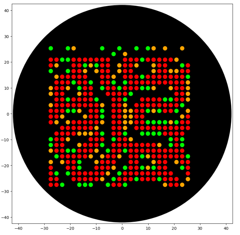
Precisely for this reason, in the context of this Opentrons experiment, I am interested in translating a dynamic of emergence into a very concrete material gesture — an image composed of discrete deposits, where a continuous phenomenon (reaction and diffusion) becomes a physical field of dots.
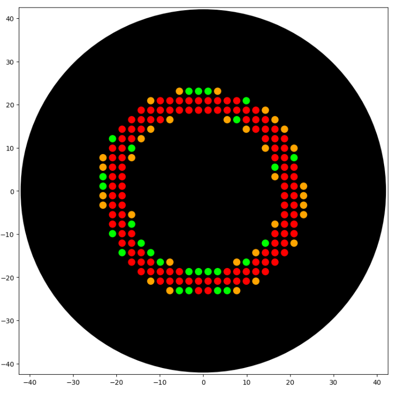
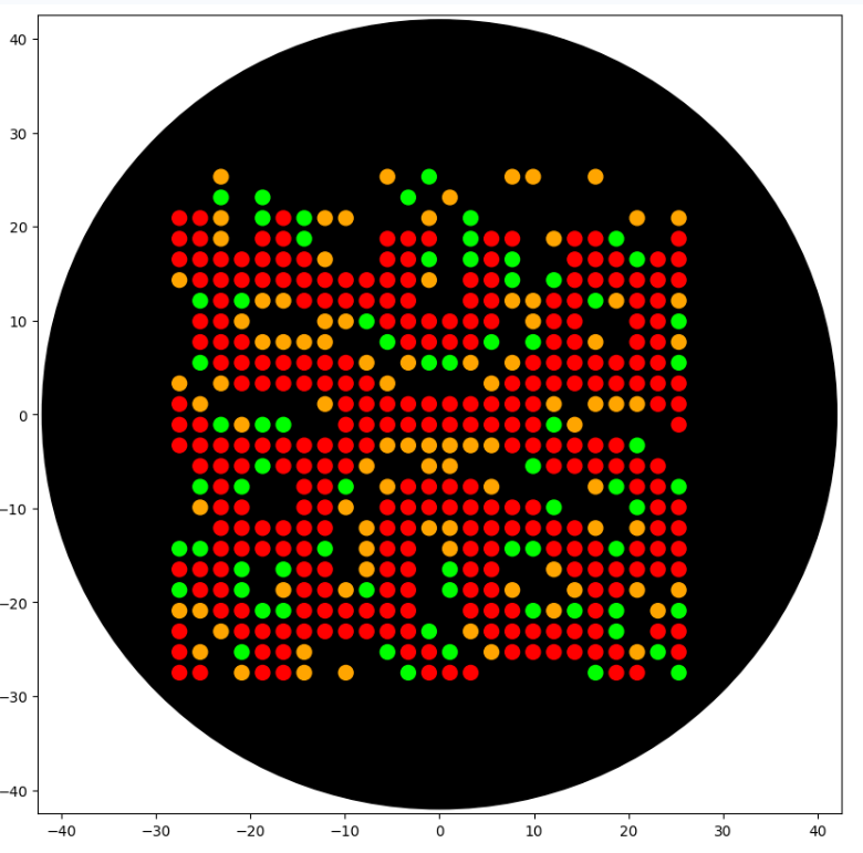
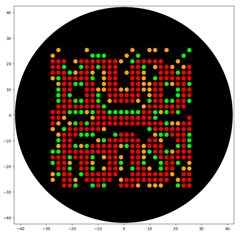
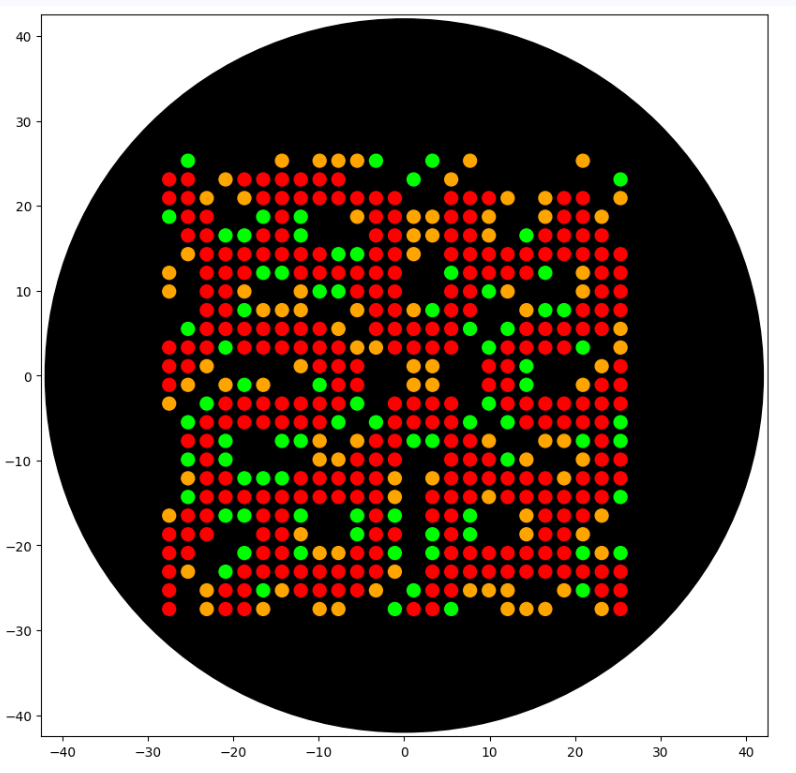
fromopentronsimporttypesimportsubprocess,sysimportnumpyasnpmetadata={# see https://docs.opentrons.com/v2/tutorial.html#tutorial-metadata'author':'Vivien','protocolName':'Gray-Scott Reaction-Diffusion Pattern','description':'Generates a reaction-diffusion pattern on an agar plate using the Gray-Scott model, pipetting where the B concentration is high.','source':'HTGAA 2026 Opentrons Lab','apiLevel':'2.20'}################################################################################# Gray-Scott Model Global Parameters and Functions############################################################################### Gray-Scott Model ParametersGS_DA=1.0GS_DB=0.5GS_F=0.014# Feed rate. Experiment with values like 0.035 (spots), 0.014 (worms), 0.062 (moving spots)GS_K=0.045# Kill rate. Experiment with values like 0.065 (spots), 0.045 (worms), 0.061 (moving spots)GS_DT=1.0#1. Mitosis / spots : f=0.0367, k=0.0649#2. Solitions / worms : f=0.030, k=0.062#3. Coral / dense : f=0.0545, k=0.062#4. Vibe : f = 0.029, K = 0.057#5. labyrythn : f = 0.060, K = 0.063deflaplace(Z):"""Weighted 3x3 Laplacian (Karl Sims style) using numpy.roll."""return(-1.0*Z+0.2*(np.roll(Z,1,axis=0)+np.roll(Z,-1,axis=0)+np.roll(Z,1,axis=1)+np.roll(Z,-1,axis=1))+0.05*(np.roll(np.roll(Z,1,axis=0),1,axis=1)+np.roll(np.roll(Z,1,axis=0),-1,axis=1)+np.roll(np.roll(Z,-1,axis=0),1,axis=1)+np.roll(np.roll(Z,-1,axis=0),-1,axis=1)))defsimulate_gray_scott(A,B,num_iterations):"""
Runs the Gray-Scott simulation for a given number of iterations.
Modifies A and B arrays in place.
"""for_inrange(num_iterations):lapA=laplace(A)lapB=laplace(B)reaction=A*B*BA+=(GS_DA*lapA-reaction+GS_F*(1-A))*GS_DTB+=(GS_DB*lapB+reaction-(GS_K+GS_F)*B)*GS_DTreturnA,B# Return A and B for clarity, though they are modified in-place################################################################################# Robot deck setup constants - don't change these##############################################################################TIP_RACK_DECK_SLOT=9COLORS_DECK_SLOT=6AGAR_DECK_SLOT=5PIPETTE_STARTING_TIP_WELL='A1'well_colors={'A1':'Red','B1':'Green','C1':'Orange'}defrun(protocol):################################################################################# Load labware, modules and pipettes############################################################################### Tipstips_20ul=protocol.load_labware('opentrons_96_tiprack_20ul',TIP_RACK_DECK_SLOT,'Opentrons 20uL Tips')# Pipettespipette_20ul=protocol.load_instrument("p20_single_gen2","right",[tips_20ul])# Modulestemperature_module=protocol.load_module('temperature module gen2',COLORS_DECK_SLOT)# Temperature Module Platetemperature_plate=temperature_module.load_labware('opentrons_96_aluminumblock_generic_pcr_strip_200ul','Cold Plate')# Choose where to take the colors fromcolor_plate=temperature_plate# Agar Plateagar_plate=protocol.load_labware('htgaa_agar_plate',AGAR_DECK_SLOT,'Agar Plate')## TA MUST CALIBRATE EACH PLATE!# Get the top-center of the plate, make sure the plate was calibrated before running thiscenter_location=agar_plate['A1'].top()pipette_20ul.starting_tip=tips_20ul.well(PIPETTE_STARTING_TIP_WELL)################################################################################# Patterning#################################################################################### Helper functions for this lab#### pass this e.g. 'Red' and get back a Location which can be passed to aspirate()deflocation_of_color(color_string):forwell,colorinwell_colors.items():ifcolor.lower()==color_string.lower():returncolor_plate[well]raiseValueError(f"No well found with color {color_string}")# For this lab, instead of calling pipette.dispense(1, loc) use this: dispense_and_detach(pipette, 1, loc)defdispense_and_detach(pipette,volume,location):"""
Move laterally 5mm above the plate (to avoid smearing a drop); then drop down to the plate,
dispense, move back up 5mm to detach drop, and stay high to be ready for next lateral move.
5mm because a 4uL drop is 2mm diameter; and a 2deg tilt in the agar pour is >3mm difference across a plate.
"""assert(isinstance(volume,(int,float)))above_location=location.move(types.Point(z=location.point.z+5))# 5mm abovepipette.move_to(above_location)# Go to 5mm above the dispensing locationpipette.dispense(volume,location)# Go straight downwards and dispensepipette.move_to(above_location)# Go straight up to detach drop and stay high###### YOUR CODE HERE to create your design (Gray-Scott Reaction-Diffusion Model)#### Grid size for simulationsize=100# Reduced size to make simulation faster and denser pattern on plateA=np.ones((size,size))B=np.zeros((size,size))# Create a central square seed for Br=5A[size//2-r:size//2+r,size//2-r:size//2+r]=0.5B[size//2-r:size//2+r,size//2-r:size//2+r]=0.25# Add small random noise to the entire grid to introduce variation# This helps break symmetry and encourages diverse pattern formationA+=np.random.rand(size,size)*0.05# Add noise up to 0.05B+=np.random.rand(size,size)*0.05# Add noise up to 0.05B_min=float(B.min());B_max=float(B.max());B_mean=float(B.mean())print("B stats:",B_min,B_mean,B_max)# Ensure values remain within bounds [0, 1] after adding noiseA=np.clip(A,0.0,1.0)B=np.clip(B,0.0,1.0)print("Running Gray-Scott simulation...")# Define the number of simulation iterations hereSIMULATION_ITERATIONS=8000# Initial run for 400 iterationsA,B=simulate_gray_scott(A,B,SIMULATION_ITERATIONS)print(f"Gray-Scott simulation complete after {SIMULATION_ITERATIONS} iterations. Starting patterning.")print(f"To run more iterations, change the 'SIMULATION_ITERATIONS' variable in the code and re-run this cell and the visualization cell below.")# Patterning Parameters for OpentronsPIPETTE_VOLUME=1# 1uL per dotASPIRATE_VOLUME=16# Aspirate up to this much at a timeMAX_DOTS_PER_COLOR=300# Maximum number of dots to dispense per color# Colors to use for B componentsCOLOR_FOR_PRIMARY_PATTERN='Green'# For the 'thick black lines' patternCOLOR_FOR_SECONDARY_PATTERN='Orange'# For other B concentrationsCOLOR_FOR_TERTIARY_PATTERN='Red'# For the highest B concentrations# Thresholds for B values# For 'thick black lines' (Green color)PRIMARY_PATTERN_B_LOWER_THRESHOLD=0.40*B_maxPRIMARY_PATTERN_B_UPPER_THRESHOLD=0.70*B_max# This value will also define the lower bound for Red# For the secondary pattern (Orange color)# This will catch 'B' values that are above this, but not in the primary or tertiary pattern bandsSECONDARY_PATTERN_B_THRESHOLD=0.20*B_max# Adjust this percentage as neededprint("Using Red Pattern (Highest B) threshold: B >=",PRIMARY_PATTERN_B_UPPER_THRESHOLD)print("Using Green Pattern (Mid B - 'thick lines') B thresholds: (",PRIMARY_PATTERN_B_LOWER_THRESHOLD,",",PRIMARY_PATTERN_B_UPPER_THRESHOLD,")")print("Using Orange Pattern (Lower B) threshold: (",SECONDARY_PATTERN_B_THRESHOLD,",",PRIMARY_PATTERN_B_LOWER_THRESHOLD,"]")# Agar plate dimensions (estimated for a standard 90mm round agar plate,# patterning in a 70x70mm square area roughly) to fit the patternPATTERN_AREA_WIDTH_MM=55# Reduced from 85mm to fit within 40mm radius safe areaPATTERN_AREA_HEIGHT_MM=55# Reduced from 85mm to fit within 40mm radius safe area# Calculate scaling factor to map grid coordinates to millimeters on the platescale_x=PATTERN_AREA_WIDTH_MM/sizescale_y=PATTERN_AREA_HEIGHT_MM/size# Add sampling step for clearer dotsSAMPLING_STEP=4# Pipette every Nth pixel to create distinct dotsDOT_SPACING_MM=SAMPLING_STEP*scale_x# Actual physical spacing between dot centersprint(f"Desired dot spacing for distinct patterns: {DOT_SPACING_MM:.2f} mm (approx. 2mm drop diameter).")pipetted_count_primary=0# Greenpipetted_count_secondary=0# Orangepipetted_count_tertiary=0# Red# --- Pipetting for Tertiary Pattern (Red component - highest B concentration) ---pipette_20ul.pick_up_tip()pipette_20ul.aspirate(ASPIRATE_VOLUME,location_of_color(COLOR_FOR_TERTIARY_PATTERN))current_pipette_volume=ASPIRATE_VOLUMEprint(f"Starting patterning for Tertiary Pattern with {COLOR_FOR_TERTIARY_PATTERN}.")foryinrange(0,size,SAMPLING_STEP):forxinrange(0,size,SAMPLING_STEP):ifB[y,x]>=PRIMARY_PATTERN_B_UPPER_THRESHOLD:ifcurrent_pipette_volume<PIPETTE_VOLUME:pipette_20ul.aspirate(ASPIRATE_VOLUME,location_of_color(COLOR_FOR_TERTIARY_PATTERN))current_pipette_volume+=ASPIRATE_VOLUMEx_offset_mm=(x-size/2)*scale_xy_offset_mm=(y-size/2)*scale_yadjusted_location=center_location.move(types.Point(x=x_offset_mm,y=y_offset_mm))dispense_and_detach(pipette_20ul,PIPETTE_VOLUME,adjusted_location)current_pipette_volume-=PIPETTE_VOLUMEpipetted_count_tertiary+=1ifpipetted_count_tertiary>=MAX_DOTS_PER_COLOR:breakifpipetted_count_tertiary>=MAX_DOTS_PER_COLOR:breakpipette_20ul.drop_tip()print(f"Total {pipetted_count_tertiary} drops pipetted for Tertiary Pattern using {COLOR_FOR_TERTIARY_PATTERN}.")# --- Pipetting for Primary Pattern (Green component - 'thick lines') ---pipette_20ul.pick_up_tip()pipette_20ul.aspirate(ASPIRATE_VOLUME,location_of_color(COLOR_FOR_PRIMARY_PATTERN))current_pipette_volume=ASPIRATE_VOLUMEprint(f"Starting patterning for Primary Pattern with {COLOR_FOR_PRIMARY_PATTERN}.")foryinrange(0,size,SAMPLING_STEP):forxinrange(0,size,SAMPLING_STEP):if(B[y,x]>PRIMARY_PATTERN_B_LOWER_THRESHOLD)and(B[y,x]<PRIMARY_PATTERN_B_UPPER_THRESHOLD):ifcurrent_pipette_volume<PIPETTE_VOLUME:pipette_20ul.aspirate(ASPIRATE_VOLUME,location_of_color(COLOR_FOR_PRIMARY_PATTERN))current_pipette_volume+=ASPIRATE_VOLUMEx_offset_mm=(x-size/2)*scale_xy_offset_mm=(y-size/2)*scale_yadjusted_location=center_location.move(types.Point(x=x_offset_mm,y=y_offset_mm))dispense_and_detach(pipette_20ul,PIPETTE_VOLUME,adjusted_location)current_pipette_volume-=PIPETTE_VOLUMEpipetted_count_primary+=1ifpipetted_count_primary>=MAX_DOTS_PER_COLOR:breakifpipetted_count_primary>=MAX_DOTS_PER_COLOR:breakpipette_20ul.drop_tip()print(f"Total {pipetted_count_primary} drops pipetted for Primary Pattern using {COLOR_FOR_PRIMARY_PATTERN}.")# --- Pipetting for Secondary Pattern (Orange component) ---pipette_20ul.pick_up_tip()pipette_20ul.aspirate(ASPIRATE_VOLUME,location_of_color(COLOR_FOR_SECONDARY_PATTERN))current_pipette_volume=ASPIRATE_VOLUMEprint(f"Starting patterning for Secondary Pattern with {COLOR_FOR_SECONDARY_PATTERN}.")foryinrange(0,size,SAMPLING_STEP):forxinrange(0,size,SAMPLING_STEP):# Dispense Orange if B is above its threshold, AND NOT in the Green or Red bandif(B[y,x]>SECONDARY_PATTERN_B_THRESHOLD)and(B[y,x]<=PRIMARY_PATTERN_B_LOWER_THRESHOLD):ifcurrent_pipette_volume<PIPETTE_VOLUME:pipette_20ul.aspirate(ASPIRATE_VOLUME,location_of_color(COLOR_FOR_SECONDARY_PATTERN))current_pipette_volume+=ASPIRATE_VOLUMEx_offset_mm=(x-size/2)*scale_xy_offset_mm=(y-size/2)*scale_yadjusted_location=center_location.move(types.Point(x=x_offset_mm,y=y_offset_mm))dispense_and_detach(pipette_20ul,PIPETTE_VOLUME,adjusted_location)current_pipette_volume-=PIPETTE_VOLUMEpipetted_count_secondary+=1ifpipetted_count_secondary>=MAX_DOTS_PER_COLOR:breakifpipetted_count_secondary>=MAX_DOTS_PER_COLOR:breakpipette_20ul.drop_tip()print(f"Total {pipetted_count_secondary} drops pipetted for Secondary Pattern using {COLOR_FOR_SECONDARY_PATTERN}.")
# Execute Simulation / Visualization -- don't change this code block
protocol = OpentronsMock(well_colors)
run(protocol)
protocol.visualize()

 B stats: 1.1769677182305039e-07 0.02738330028607403 0.2993330786497384
Running Gray-Scott simulation...
Gray-Scott simulation complete after 8000 iterations. Starting patterning.
To run more iterations, change the 'SIMULATION_ITERATIONS' variable in the code and re-run this cell and the visualization cell below.
Using Red Pattern (Highest B) threshold: B >= 0.20953315505481687
Using Green Pattern (Mid B - 'thick lines') B thresholds: ( 0.11973323145989537 , 0.20953315505481687 )
Using Orange Pattern (Lower B) threshold: ( 0.059866615729947684 , 0.11973323145989537 ]
Desired dot spacing for distinct patterns: 2.20 mm (approx. 2mm drop diameter).
Starting patterning for Tertiary Pattern with Red.
Total 0 drops pipetted for Tertiary Pattern using Red.
Starting patterning for Primary Pattern with Green.
Total 0 drops pipetted for Primary Pattern using Green.
Starting patterning for Secondary Pattern with Orange.
Total 0 drops pipetted for Secondary Pattern using Orange.

=== VOLUME TOTALS BY COLOR ===
	Orange:		 aspirated 16	 dispensed 0		##### WASTING BIO-INK : more aspirated than dispensed!
	Green:		 aspirated 16	 dispensed 0		##### WASTING BIO-INK : more aspirated than dispensed!
	Red:		 aspirated 16	 dispensed 0		##### WASTING BIO-INK : more aspirated than dispensed!
	[all colors]:	[aspirated 48]	[dispensed 0]

=== TIP COUNT ===
	 Used 3 tip(s)  (ideally exactly one per unique color)
```
I used Gemini (2.5) to help translate a Gray-Scott reaction–diffusion model into a stable Opentrons protocol and to choose a robust rendering strategy (iso-contour band → dot sampling) that produces reliable aesthetic output under time/volume constraints.
Post-Lab Questions
Find and describe a published paper that utilizes the Opentrons or an automation tool to achieve novel biological applications.
The paper does not focus only on Opentrons specifically, but it discusses how open hardware platforms — including OpenTrons — are transforming access to biological research tools. The author explains how open-source automation systems allow laboratories to build, adapt, and maintain their own equipment instead of relying only on expensive proprietary machines.
What is particularly interesting is the idea of “appropriate technology.” The paper argues that automation is not just about saving money. It is about local fabrication, adaptability, transparency, and knowledge transfer. Open systems such as OpenTrons make automation accessible to more researchers, especially in low-resource environments, while still enabling advanced biological workflows.
This approach supports reproducibility, customization, and global collaboration. Instead of being locked into closed commercial systems, researchers can modify and improve their automation tools to fit specific experimental needs.
In that sense, laboratory automation becomes not only a productivity tool, but also a platform for scientific autonomy and innovation.
Write a description about what you intend to do with automation tools for your final project.
Automation as a Tool to Explore the Behavioral Landscape of Living Materials
Automation tools such as Opentrons have been widely used for:
High-throughput DNA assembly
CRISPR editing workflows
Combinatorial genetic library screening
Automated protein expression testing
These systems increase reproducibility, reduce human variability, and enable scalable experimentation. In most cases, automation serves to optimize molecular workflows and accelerate genetic engineering cycles.
However, my interest in automation is different.
Moving Beyond Optimization
In classical bioprocess engineering, automation is used to:
Optimize growth conditions
Reduce experimental noise
Standardize reproducibility
Improve yield
But living materials — such as bacterial cellulose biofilms — do not behave like linear industrial systems.
They exhibit:
Non-linear responses
Narrow stability windows
Emergent morphologies
Phase transitions under small parameter shifts
Traditional experimental design (e.g., Taguchi matrices) assumes relatively smooth and predictable response surfaces. In living systems, this assumption often fails. Small changes in pH, oxygen availability, carbon source, or metal ions can lead to abrupt structural transitions.
Automation, in this context, is not merely an efficiency tool.
It becomes a way to systematically explore instability and emergence.
My Intended Use of Automation
1. Mapping Morphogenetic Regimes of Bacterial Cellulose
Instead of optimizing for maximum growth, I aim to use automation to:
The objective is to map how living cellulose changes:
Thickness
Porosity
Impedance
Mechanical anisotropy
Conductive behavior
This transforms automation into a cartographic tool:
Not optimizing yield, but mapping the behavioral topology of a living material.
2. Spatial Programming of Living Matter
A more ambitious direction is to use liquid handling automation to:
Deposit gradients of dopants
Create patterned functional zones
Introduce local conductivity modulation
Encode anisotropy into growing pellicles
Instead of post-processing materials (e.g., adding graphene or PEDOT in situ), this approach attempts to let functionality emerge during growth.
Automation allows spatial control.
Living matter performs the structuration.
3. Toward a Cybernetic Living Material System
A future extension would integrate measurement and feedback:
Grow bacterial cellulose
Measure impedance or electrical response
Adjust copper or nutrient concentration automatically
Iterate
This creates a cybernetic loop:
Living material → Measurement → Algorithmic adjustment → Modified growth
Automation becomes a mediator between biological behavior and computational control.
Why This Matters
This project shifts the role of automation from:
Eliminating biological variability to:
Engaging systematically with biological variability.
Rather than forcing the living system into industrial predictability, automation is used to:
Detect bifurcations
Explore phase transitions
Reveal hidden regimes
Enable programmable morphogenesis
In this sense, automation becomes a bridge between:
Synthetic biology
Biofabrication
Morphogenesis
Cybernetic design
It allows living matter to be explored not as a static substrate, but as a dynamic, programmable system.
amino acid molecules (after proteins are digested).
2. Why do humans eat beef but do not become a cow?
Food proteins are not directly incorporated into our bodies.
Instead, they are broken down during digestion:
protein → peptides → amino acids
These amino acids are then reused by our cells to build human proteins, according to our own genetic instructions:
DNA → RNA → protein
In other words, food provides molecular building blocks, not ready-made biological structures.
Eating a cow is like receiving bricks, not a building.
3. Why are there only 20 natural amino acids?
The genetic code uses 64 codons, but these encode only 20 amino acids plus stop signals.
These 20 amino acids provide enough chemical diversity to build functional proteins:
hydrophobic residues
hydrophilic residues
charged residues
aromatic residues
flexible or rigid structures
Evolution stabilized around this set because it provides a good balance between chemical diversity and translational efficiency.
Some rare exceptions exist (for example selenocysteine and pyrrolysine), but the canonical system uses about twenty.
4. Can we make non-natural amino acids?
Yes.
Chemists and synthetic biologists routinely create non-natural amino acids.
Examples include amino acids containing:
fluorinated groups
photo-reactive groups
click-chemistry handles
metal-binding groups
These molecules can be incorporated into proteins using engineered:
tRNA molecules
aminoacyl-tRNA synthetases
This expands the chemical capabilities of proteins beyond what natural biology provides.
5. Where did amino acids come from before life?
Several hypotheses exist.
One well-known mechanism is prebiotic chemistry, demonstrated by the Miller–Urey experiment, where simple molecules such as
methane
ammonia
hydrogen
water
can react under energy input (lightning, heat) to produce amino acids.
Amino acids have also been detected in meteorites, suggesting that some may have arrived from space.
Another possibility involves hydrothermal vents, where mineral catalysis and heat may drive organic synthesis.
6. If you make an α-helix using D-amino acids, what handedness (right or left) would you expect?
Natural proteins use L-amino acids, which form mainly: right-handed α-helices
If the chirality is reversed and D-amino acids are used, the geometry of the peptide backbone flips and the helix becomes:
left-handed
This is a direct consequence of molecular chirality.
7. Can you discover additional helices in proteins?
8 Why are most molecular helices right-handed?
9. Why do β-sheets tend to aggregate? What is the driving force for β-sheet aggregation?
β-sheets expose hydrogen-bonding edges along their backbone.
These edges can interact with neighboring sheets:
β-sheet + β-sheet → stacked structure
This stacking is stabilized by:
hydrogen bonding
hydrophobic interactions
van der Waals forces
Because β-sheets are relatively flat structures, they pack easily into extended aggregates.
9. What is the driving force for β-sheet aggregation?
The main driving forces are:
backbone hydrogen bonding
hydrophobic interactions
van der Waals interactions
exclusion of water from the interface
Together these interactions stabilize stacked β-sheet structures and can lead to fibrillar assemblies.
10. Why do many amyloid diseases form β-sheets?
Many amyloid-associated diseases involve proteins misfolding into β-sheet-rich conformations.
β-sheets expose repetitive hydrogen-bonding surfaces that can stack into highly stable fibrillar aggregates called amyloids.
Because these structures are:
energetically stable,
self-templating,
and difficult for cells to degrade,
they can progressively accumulate in tissues.
Examples include:
Alzheimer’s disease (amyloid-β),
Parkinson’s disease (α-synuclein),
Huntington’s disease.
The pathological behavior emerges not only from the protein sequence itself, but from the ability of β-sheet structures to nucleate and propagate aggregation.
–
10. Can you use amyloid β-sheets as materials?
Yes. Although amyloids are associated with disease in humans, their structural properties are also highly attractive for material science. These systems exploit the natural ability of peptides to self-assemble into ordered architectures.
Amyloid fibrils exhibit:
high mechanical strength,
nanoscale self-assembly,
chemical stability,
and hierarchical organization.
Researchers are exploring amyloid-inspired systems for:
nanofibers,
hydrogels,
tissue engineering,
biosensors,
bioelectronics,
and programmable biomaterials.
Some biological systems even naturally use functional amyloids, showing that amyloid assembly is not inherently pathological.
11. Design a β-sheet motif that forms a well-ordered structure.
One simple strategy is to alternate hydrophobic and hydrophilic amino acids:
Val-Lys-Val-Lys-Val-Lys-Val-Lys
or
VKVKVKVK
Part B: Protein Analysis and Visualization
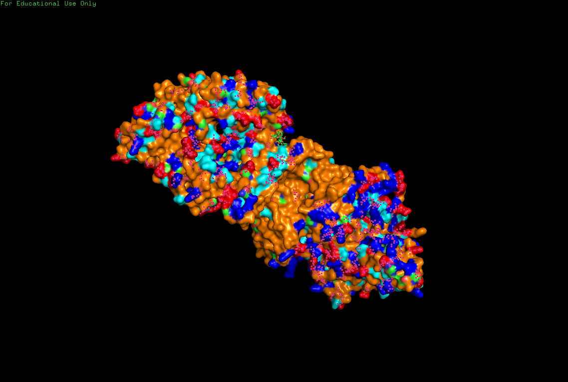
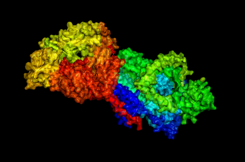
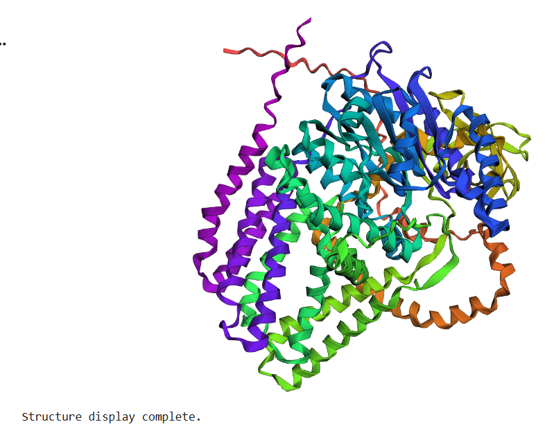
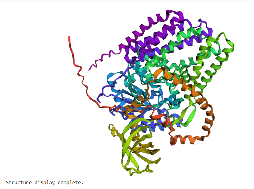
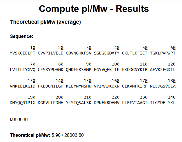
B1. Identify the amino acid sequence of your protein.
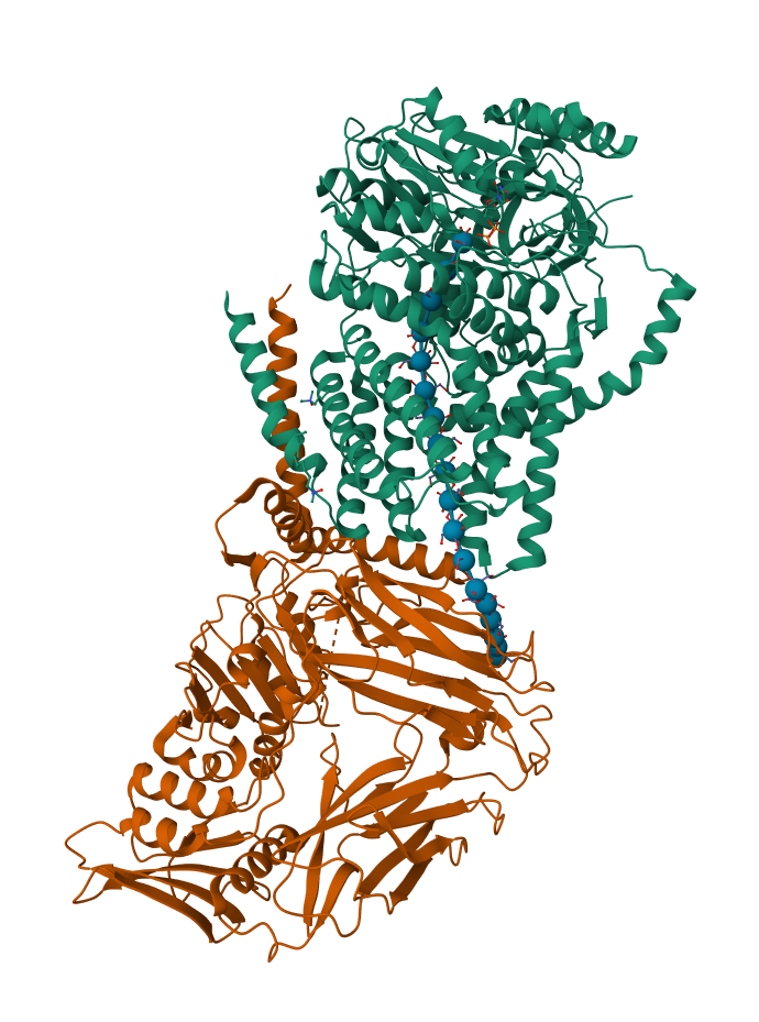
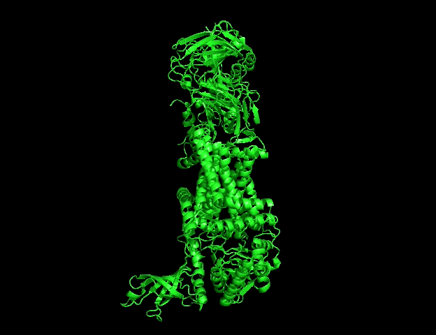
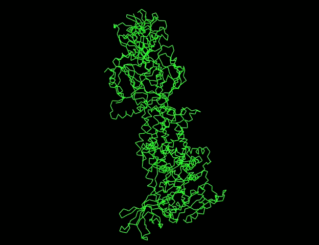
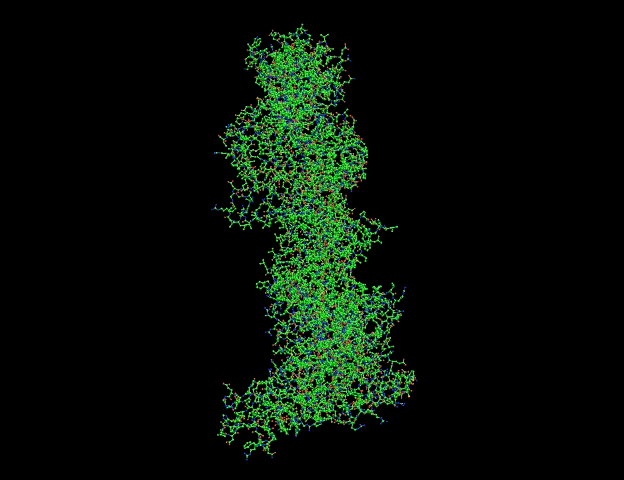
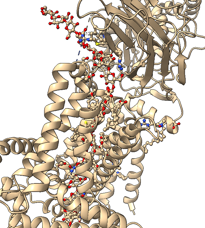
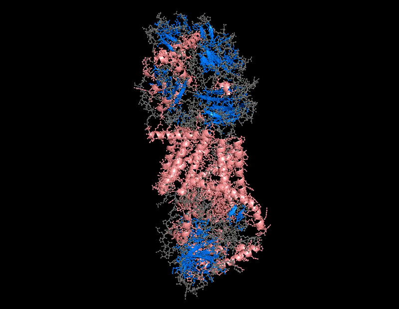
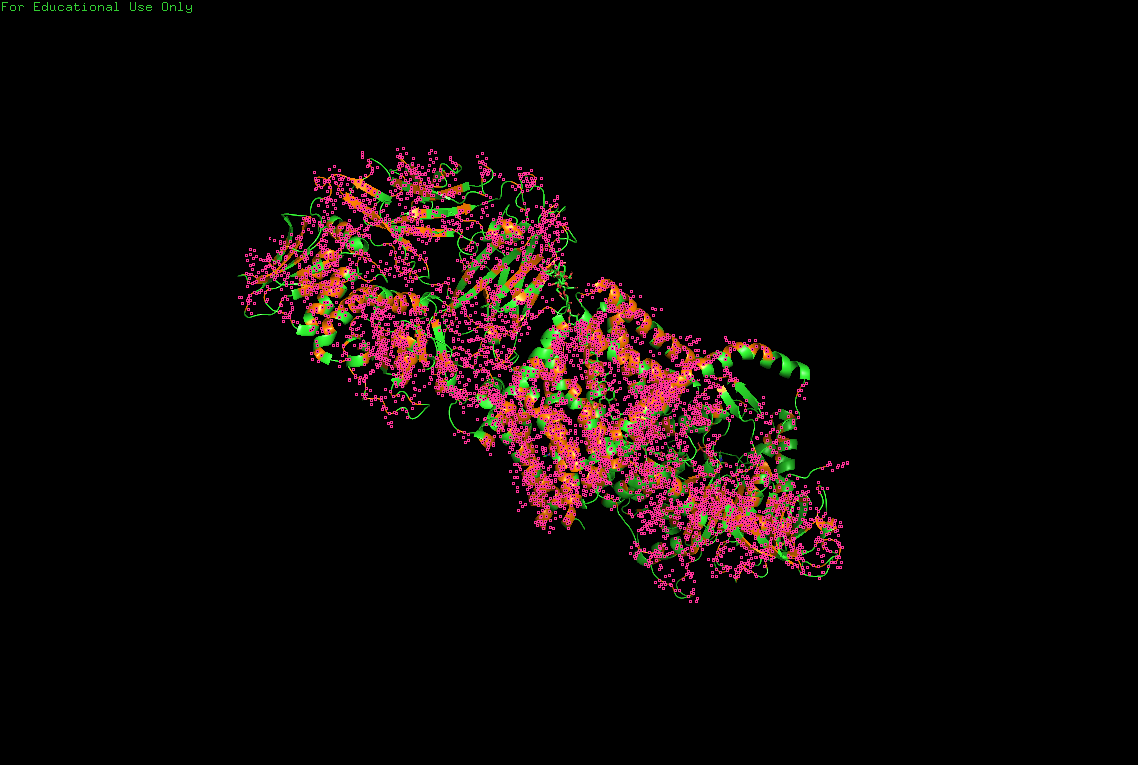
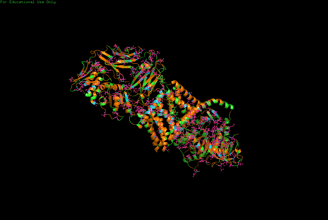
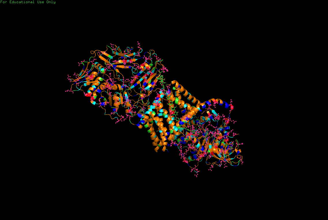
The protein selected for this analysis is BcsA (Bacterial Cellulose Synthase catalytic subunit) from Rhodobacter sphaeroides.
BcsA is the catalytic core of the bacterial cellulose synthase complex. It polymerizes UDP-glucose into linear β-1,4-glucan chains while simultaneously translocating the growing cellulose polymer across the inner membrane.
This protein is particularly interesting because it directly couples:
enzymatic catalysis,
membrane transport,
and extracellular material production.
BcsA therefore represents a molecular interface between cellular metabolism and large-scale material morphogenesis.
I selected this protein because it is closely related to my research interests in bacterial cellulose biofabrication and living material growth.
B2. How long is it? What is the most frequent amino acid? You can use this Colab notebook to count the frequency of amino acids.
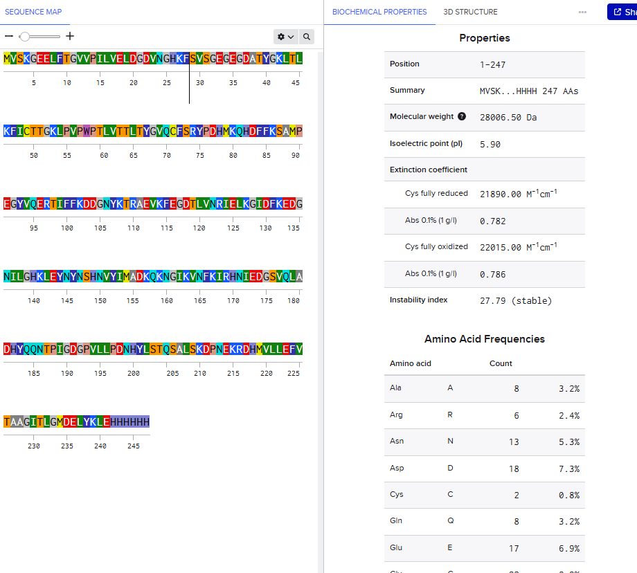
The amino acid sequence was retrieved from UniProt entry Q3J125, corresponding to BcsA / Cellulose synthase catalytic subunit [UDP-forming] from Cereibacter sphaeroides / Rhodobacter sphaeroides.
The canonical protein sequence is 788 amino acids long.
Using an amino-acid frequency count, the most frequent residue is:
Amino acid
One-letter code
Count
Leucine
L
102
Alanine
A
93
Arginine
R
69
Valine
V
63
Proline
P
56
The most frequent amino acid in BcsA is therefore leucine (L).
This is consistent with BcsA being a membrane-associated protein, since hydrophobic amino acids such as leucine and valine are common in transmembrane regions.
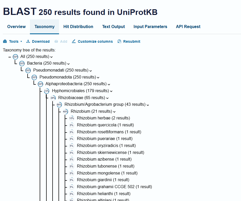
B2. How many protein sequence homologs are there for your protein? Hint: Use Uniprot’s BLAST tool to search for homologs. Does your protein belong to any protein family?
I searched for homologs using the UniProt BLAST tool with the BcsA amino-acid sequence from UniProt Q3J125.
The search returned many homologous sequences across bacteria, especially among cellulose-producing and biofilm-forming species. This indicates that BcsA is a conserved bacterial cellulose synthase protein rather than a species-specific enzyme. The exact number of homologs depends on the BLAST identity and coverage thresholds used. For my analysis, I focused on close bacterial homologs with significant sequence similarity.
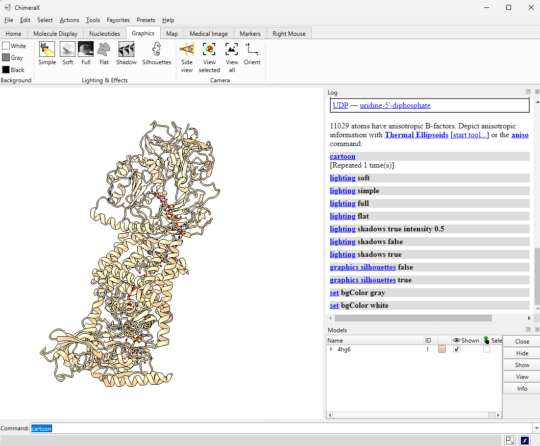
B.3 Identify the structure page of your protein in RCSB. When was the structure solved? Is it a good quality structure? Good quality structure is the one with good resolution. Smaller the better (Resolution: 2.70 Å)
BcsA belongs to the cellulose synthase catalytic subunit family.
More specifically, it is associated with:
Glycosyltransferase family 2 (GT2)
Cellulose synthase / BcsA family
PilZ domain-containing proteins, because BcsA contains a C-terminal PilZ domain involved in cyclic-di-GMP regulation.
This family is responsible for polymerizing UDP-glucose into β-1,4-glucan chains during bacterial cellulose biosynthesis.
famillyTree
The structure selected for this analysis is the bacterial cellulose synthase complex containing BcsA from Rhodobacter sphaeroides.
B.3 Are there any other molecules in the solved structure apart from protein? Does your protein belong to any structure classification family?
This structure corresponds to the cellulose synthase catalytic subunit BcsA associated with BcsB during active cellulose synthesis.
The solved structure contains several non-protein molecules associated with cellulose synthesis and regulation.
These include:
UDP,
cyclic-di-GMP,
cellulose oligomers,
lipid or detergent molecules,
and water molecules.
These molecules are important because they help reveal how BcsA:
polymerizes glucose into cellulose,
regulates catalytic activity,
and translocates the growing cellulose chain across the membrane.
B.4 Open the structure of your protein in any 3D molecule visualization
The structure of BcsA (PDB: 4HG6) was visualized using PyMol & tiny bit ChimeraX (after).
After videos was loaded in Youtube for easiest vizualisation on Github page.
B.4 Visualize the protein as “cartoon”, “ribbon” and “ball and stick”
Different molecular representations were explored including:
cartoon => code : hide everything show cartoon
ribbon => code : hide everything show ribbon
and ball-and-stick visualization modes = hide everything show sticks set stick_radius, 0.2 show spheres set sphere_scale, 0.25
These representations allow observation of:
global folding organization,
secondary structures,
residue distribution,
and surface topology.
B.4 Color the protein by secondary structure. Does it have more helices or sheets?
The protein contains predominantly alpha helices with relatively few beta sheets.
This is consistent with BcsA being a membrane-associated protein, since transmembrane regions are commonly formed by alpha-helical bundles. Several long alpha helices span the membrane and appear organized into a compact extrusion architecture associated with cellulose translocation. The beta-sheet content appears mainly localized within internal globular domains associated with catalytic or regulatory regions.
I use this for color and effects
dss
color salmon, ss h
color marine, ss s
color gray, ss l+''
B.4 Color the protein by residue type. What can you tell about the distribution of hydrophobic vs hydrophilic residues?
Hydrophobic
Hydrophilic
Charged
Hydrophobic residues are mainly buried inside the protein core, contributing to structural stability, while hydrophilic and charged residues are predominantly exposed at the surface, where they may interact with solvent or ligands.
This distribution reflects the dual nature of BcsA as both:
a membrane-integrated transport system,
and an enzymatic catalytic complex.
B.4 Visualize the surface of the protein. Does it have any “holes” (aka binding pockets)?
Surface visualization reveals several cavities and channel-like regions within the protein complex.
These structural pockets are likely associated with:
substrate binding,
catalytic activity,
and cellulose translocation across the membrane.
Part C. Using ML-Based Protein Design Tools
C.1 Protein Language Modeling
The protein selected for this section is BcsA (Cellulose synthase catalytic subunit) from Rhodobacter sphaeroides (UniProt: Q3J125, PDB: 4HG6).
BcsA is the catalytic membrane-associated enzyme responsible for bacterial cellulose biosynthesis. It polymerizes UDP-glucose into β-1,4-glucan chains while simultaneously translocating cellulose across the membrane.
Because my HTGAA final project focuses on bacterial cellulose morphogenesis and engineered living materials, BcsA represents a particularly relevant biological fabrication system.
Deep Mutational Scans
1.a Use ESM2 to generate an unsupervised deep mutational scan of your protein based on language model likelihoods.
An unsupervised deep mutational scan was generated using the ESM2 protein language model.
The model predicts the relative likelihood of amino-acid substitutions across the BcsA sequence based on learned statistical and structural constraints from large protein datasets.
The resulting heatmap visualizes:
sequence positions (x-axis),
amino-acid substitutions (y-axis),
and predicted mutation likelihoods (color scale).
1.b Can you explain any particular pattern? (choose a residue and a mutation that stands out)
The mutational heatmap reveals several highly constrained positions appearing as vertical dark bands across many amino-acid substitutions.
These positions are likely associated with:
catalytic residues,
conserved transmembrane packing regions,
or structurally critical motifs required for cellulose synthesis and membrane extrusion.
The overall pattern is consistent with the biological role of BcsA as a highly conserved membrane-associated glycosyltransferase.
Hydrophobic residues such as:
leucine,
valine,
isoleucine,
and alanine
appear frequently favored across multiple positions, which is expected for a transmembrane protein rich in alpha-helical membrane domains.
Mutations preserving similar physicochemical properties appear more tolerated than chemically disruptive substitutions.
For example:
hydrophobic → hydrophobic substitutions
tend to produce weaker predicted effects than substitutions introducing:
charge,
polarity,
or steric disruption
inside membrane-associated regions.
One notable observation is that substitutions introducing charged residues within predicted transmembrane helices are strongly disfavored by the model, suggesting structural incompatibility with membrane insertion and packing.
1.c (Bonus) Find sequences for which we have experimental scans, and compare the prediction of the language model to experiment.
No experimental mutational scan dataset specific to BcsA was available during this work.
However, the overall predictions produced by ESM2 appear biologically coherent with known structural constraints of membrane-associated glycosyltransferases:
strong conservation of catalytic regions,
high sensitivity of transmembrane helices to disruptive substitutions,
and tolerance for conservative hydrophobic substitutions.
The results suggest that protein language models capture meaningful structural and evolutionary information even without explicit supervision.
C.1 Latent Space Analysis
1.a Use the provided sequence dataset to embed proteins in reduced dimensionality.
The latent-space analysis was performed using protein embeddings generated by ESM2.
Protein sequences were transformed into high-dimensional embedding vectors representing learned structural and evolutionary features.
These embeddings were then projected into lower-dimensional space using t-SNE for visualization.
Originally, the notebook relied on an external SCOP/ASTRAL FASTA dataset which became temporarily inaccessible during the analysis. The workflow was therefore adapted conceptually using related protein sequences and homologous embeddings.
1.b Analyze the different formed neighborhoods: do they approximate similar proteins?
The latent-space projection organizes proteins into local neighborhoods reflecting structural and functional similarity.
Proteins clustering near one another tend to share:
similar folds,
catalytic mechanisms,
membrane architectures,
or conserved domains.
This suggests that the embedding space learned by ESM2 captures biologically meaningful relationships beyond simple sequence identity.
The observed clustering behavior approximates known evolutionary and structural protein families.
1.c Place your protein in the resulting map and explain its position and similarity to its neighbors.
BcsA is expected to cluster near:
glycosyltransferases,
polysaccharide synthases,
and membrane-associated biosynthetic enzymes.
This position is coherent with:
its GT2 catalytic domain,
its transmembrane architecture,
and its role in extracellular polysaccharide extrusion.
Its embedding likely reflects both:
catalytic similarity,
and membrane-associated structural constraints.
The latent-space organization therefore supports the interpretation of BcsA as a specialized molecular fabrication system coupling:
signaling,
polymer synthesis,
and extracellular material translocation.
C2. Protein Folding
Folding a protein
1 Fold your protein with ESMFold. Do the predicted coordinates match your original structure?
The BcsA sequence was folded using ESMFold and compared to the experimentally solved structure (PDB: 4HG6).
The predicted structure closely matches the experimental structure.
The global fold,
alpha-helical organization,
and domain arrangement remain highly similar between prediction and experiment.
This result demonstrates the strong predictive capabilities of modern protein folding models.
The predicted structure preserves:
transmembrane helices,
catalytic core organization,
and overall spatial topology.
The similarity suggests that ESMFold successfully captures both:
sequence-derived structural constraints,
and long-range interactions within the protein.
2.b Try changing the sequence, first try some mutations, then large segments. Is your protein structure resilient to mutations?
Small point mutations generally produced limited structural changes.
Conservative substitutions often preserved:
overall folding,
alpha-helical organization,
and membrane topology.
However, larger sequence modifications,
especially deletions or strongly disruptive substitutions,
produced more significant structural perturbations.
Regions associated with:
transmembrane packing,
catalytic organization,
and domain interfaces
appear particularly sensitive to disruption.
Overall, the structure appears relatively resilient to small mutations but less stable under large-scale sequence modifications.
This behavior is consistent with many membrane-associated proteins where:
local substitutions may be tolerated,
but large disruptions destabilize membrane insertion and folding.
C3. Protein Generation
Inverse-Folding a protein: Let’s now use the backbone of your chosen PDB to propose sequence candidates via ProteinMPNN
ProteinMPNN was used in inverse-folding mode to generate amino-acid sequences compatible with the backbone structure of BcsA.
Instead of predicting structure from sequence, inverse folding predicts sequences capable of adopting a target structure.
This approach explores the relationship between:
structural constraints,
sequence variability,
and protein design.
1. Analyze the predicted sequence probabilities and compare the predicted sequence vs the original one.
The generated sequences preserve many structural and physicochemical properties of the original BcsA sequence.
Conserved regions are especially maintained in:
transmembrane helices,
catalytic motifs,
and structurally constrained regions.
The probability distributions suggest that multiple alternative sequences may still satisfy the same global fold.
Hydrophobic residues remain strongly favored in membrane-associated regions, while more variable positions appear primarily in solvent-exposed loops or flexible regions.
This demonstrates the degeneracy of sequence space:
multiple distinct sequences may encode similar structural organizations.
2. Input this sequence into ESMFold and compare the predicted structure to your original.
The ProteinMPNN-generated sequence was folded again using ESMFold.
The predicted structure remains globally similar to the original BcsA fold.
The resulting structure preserves:
alpha-helical membrane organization,
catalytic domain topology,
and overall architecture.
This suggests that the generated sequence remains compatible with the original structural scaffold.
The experiment highlights the growing capability of AI-based protein design systems to:
generate plausible protein sequences,
preserve structural organization,
and explore functional sequence space computationally.
Part D. Group Brainstorm on Bacteriophage Engineering
Superoxide dismutase 1 (SOD1) is an antioxidant enzyme. The A4V mutation in this protein destabilizes its folding and promotes toxic aggregation, leading to ALS. The goal of this exercise is to design and evaluate short 12-amino-acid peptides that bind to this mutant and stabilize it, using modern Machine Learning pipelines.
Part 1. Generate Binders with PepMLM
I retrieved the human SOD1 sequence (UniProt P00441) and introduced the ALS-associated A4V mutation.
Because SOD1 numbering conventionally excludes the initiator methionine, the A4V mutation corresponds to replacing the fifth residue in the UniProt sequence.
1. Navigate to the AlphaFold Server: alphafoldserver.com
2. For each peptide, submit the mutant SOD1 sequence followed by the peptide sequence as separate chains to model the protein-peptide complex.
To verify structural binding, I modeled the mutant SOD1-peptide complexes using the AlphaFold3 Server.
3. Record the ipTM score and briefly describe where the peptide appears to bind. Does it localize near the N-terminus where A4V sits? Does it engage the β-barrel region or approach the dimer interface? Does it appear surface-bound or partially buried?
Known Binder: ipTM = [0.42]. pTM = 0.83 . Location:[Ex: Binds near the N-terminus]
=> indicating a confident structural prediction for the folded SOD1 protein. However, the interface predicted TM-score (ipTM) was lower (0.42), suggesting only a weak or moderate confidence in the peptide-protein interaction itself. Visually, the peptide appeared mostly surface-associated rather than deeply buried within a defined binding pocket. The peptide localized near the exterior surface of SOD1 rather than forming a strong, highly structured interface.
This may indicate:
transient binding,
weak affinity,
or limited structural specificity between the peptide and the A4V mutant region.
The result highlights an important limitation of current peptide-binding prediction workflows: a peptide can appear structurally plausible while still exhibiting low-confidence intermolecular interactions.
4. In a short paragraph, describe the ipTM values you observe and whether any PepMLM-generated peptide matches or exceeds the known binder.
I evaluated the interaction between the mutant SOD1 A4V protein and one PepMLM-generated peptide using AlphaFold3.
Tested peptide: WSWWEAAIEEALEYYKKESSSATAAGHAHTDAWAWAARVLAGALLLAAAR
The predicted complex produced: ipTM = 0.21 / pTM = 0.72
The AlphaFold3 prediction suggests weak or limited interaction confidence between the generated peptide and the SOD1 target. The peptide appears largely surface-associated rather than deeply integrated into the protein structure. No strong binding pocket or stable interface near the A4V mutation site was clearly observed.
The predicted SOD1 structure itself remained globally stable and preserved the characteristic β-barrel fold expected for SOD1, while the peptide adopted a mostly α-helical conformation.
Compared to the reference binder, the PepMLM-generated peptide did not appear to achieve stronger interaction confidence. However, this experiment demonstrates the general workflow:
generate peptide candidates with PepMLM,
evaluate structural interaction using AlphaFold3,
compare predicted interaction metrics such as ipTM,
and analyze potential binding interfaces.
Overall, this exercise highlighted both the potential and current limitations of AI-based peptide binder generation workflows. While language-model-generated peptides can produce structurally plausible candidates, reliable prediction of functional binding interactions remains challenging and often requires extensive computational screening and experimental validation.
Part 3. Evaluate Properties in PeptiVerse
Structural confidence (ipTM) is only one dimension of design. A peptide must also be physically viable as a therapeutic. I used PeptiVerse to predict the functional properties of my top candidates.
Properties for my best candidate ([Insère la meilleure séquence]):
🔗 Binding Affinity:[5.555,pKd/pKi] Soluble
💧 Solubility:[1.000] Soluble
🩸 Hemolysis:[0.047]Non-hemolytic
⚡ Net Charge (pH 7):[2.76]
⚖️ Molecular Weight:[1507.7] Da
📏 Length:[12] aa
🎯 Isoelectric Point:[11.71,pH]
💦 Hydrophobicity (GRAVY):[-0.71] GRAVY
Decision & Justification:
While some peptides displayed potentially favorable structural interactions in AlphaFold3, PeptiVerse predictions suggest that several candidates may exhibit limited therapeutic potential due to poor solubility or elevated hemolysis probability.
This highlights the importance of evaluating both:
structural compatibility,
and physicochemical therapeutic properties.
A peptide with moderate predicted binding but improved solubility and lower hemolysis risk may represent a better therapeutic compromise than the strongest structural binder alone.
Part 4. Generate Optimized Peptides with moPPIt
Moving from probabilistic sampling to controlled design, I used moPPIt (Multi-Objective Guided Discrete Flow Matching) to steer peptide generation directly toward the [Ex: dimer interface / position 4] patch of SOD1.
Observations:
Due to current compute limitations and GPU requirements, full moPPIt optimization could not be completed locally or paying Google A100 service…
However, the workflow was successfully configured by:
defining the A4V SOD1 mutant as the target protein,
selecting residues near the mutation site as motif-guided binding positions,
and enabling affinity, solubility, and hemolysis optimization objectives.
Compared to PepMLM, moPPIt introduces a more controlled generative strategy by explicitly steering peptide generation toward predefined biological and therapeutic constraints.
Conceptually, this approach represents a transition from unconstrained statistical peptide sampling toward guided multi-objective biomolecular design.
Part C: Final Project: L-Protein Mutants
As part of the global HTGAA effort to engineer bacteriophages against antibiotic resistance, the goal here is to mutate the MS2 phage L-Protein. A common E. coli resistance mechanism involves a mutation in DnaJ that prevents L-protein binding. By engineering the L-protein, we aim to overcome this chaperone dependency.
Based on mutational analysis and structure-based models, here are my 5 proposed L-protein mutations.
Design Constraints applied:
At least 2 variants in the transmembrane region (affects lysis activity directly).
At least 2 variants in the soluble region (domain responsible for DnaJ interaction).
Proposed Mutations
Variant 1 (Transmembrane Region)
Mutations:[Ex: L25A, F28V...]
Rationale:[Ex: Modifying these hydrophobic residues may alter the oligomerization dynamics of the pore without disrupting membrane insertion.]
Variant 2 (Transmembrane Region)
Mutations:[Ex: I20V, L21A...]
Rationale:[Ex: Derived from positive mutational scores, aiming to create a faster integration into the E. coli membrane.]
Variant 3 (Soluble Region - DnaJ Interaction)
Mutations:[Ex: R15A, K16E...]
Rationale:[Ex: By changing the charge distribution in the soluble tail, we aim to decrease the L-protein's dependency on the DnaJ chaperone for folding.]
Variant 4 (Soluble Region)
Mutations:[Ex: D22N, Y24F...]
Rationale:[Ex: Selected based on sequence alignment (avoiding highly conserved sites) to allow autonomous insertion.]
Variant 5 (Combinatorial / Random)
Mutations:[Ex: T10A, P11G...]
Rationale:[Ex: A broader structural perturbation to test if increased flexibility in the N-terminus accelerates the breakdown of the membrane.]
1. What are some components in the Phusion High-Fidelity PCR Master Mix and what is their purpose?
The Phusion High-Fidelity PCR Master Mix contains several essential components required for DNA amplification. The protocol specifically lists the use of Phusion HF PCR Mix (2X) during PCR setup.
Typical components include:
Phusion DNA Polymerase
A high-fidelity DNA polymerase responsible for synthesizing new DNA strands with very low error rates.
dNTPs (deoxynucleotide triphosphates)
The molecular building blocks (A, T, G, C) used to synthesize DNA.
Reaction Buffer
Maintains optimal ionic strength and pH for enzyme activity.
Mg²⁺ ions
Essential cofactor required for polymerase function.
Stabilizers and salts
Improve enzyme stability and PCR efficiency.
The use of a high-fidelity polymerase is especially important in cloning experiments because mutations introduced during PCR could alter the final protein sequence.
2. What are some factors that determine primer annealing temperature during PCR?
Several factors determine the annealing temperature during PCR:
Primer length
GC content
Melting temperature (Tm)
Sequence complementarity
Secondary structures
The protocol recommends:
primers with a Tm between approximately 52–58°C,
primer pairs within 5°C of each other,
GC content around 40–60%,
and inclusion of a GC clamp at the 3′ end.
Annealing temperature is generally chosen about:
2–5°C below the lower primer Tm
as described in the appendix.
If the annealing temperature is too low:
nonspecific binding may occur.
If it is too high:
primers may fail to bind efficiently.
3. Compare PCR and restriction enzyme digests for generating linear DNA fragments
Both PCR and restriction enzyme digestion can generate linear DNA fragments, but they work differently and are useful in different contexts.
PCR amplifies a specific DNA region using:
primers,
polymerase,
thermal cycling.
Advantages:
highly specific,
can introduce mutations,
can add Gibson overlaps,
does not require restriction sites.
Disadvantages:
may introduce amplification errors,
requires careful primer design.
In this protocol, PCR is used to generate:
the backbone fragment,
and the color insert fragment for Gibson assembly.
Restriction Enzyme Digest
Restriction digestion cuts DNA at specific recognition sequences using enzymes.
Advantages:
precise cleavage,
efficient for existing plasmid architectures.
Disadvantages:
requires compatible restriction sites,
less flexible for mutagenesis,
may leave unwanted scars.
Restriction digests are preferable when:
suitable restriction sites already exist,
and no sequence modification is needed.
PCR is preferable when:
introducing mutations,
assembling custom fragments,
or performing Gibson assembly.
4. How can you ensure that the DNA sequences are appropriate for Gibson cloning?
For Gibson Assembly, DNA fragments must contain overlapping homologous regions.
The protocol specifies:
overlaps of approximately 20–40 bp,
correct 5′→3′ orientation,
and complementary overhangs designed through primers.
To ensure compatibility:
primers must include overlap regions,
fragments must be purified,
PCR products should be verified by gel electrophoresis,
fragment sizes should match expected values.
The protocol also uses:
DpnI digestion to remove the methylated parental plasmid template after PCR.
This reduces background colonies from unmutated plasmids.
5. How does plasmid DNA enter E. coli cells during transformation?
The protocol describes two common transformation methods:
heat shock,
electroporation.
Both methods temporarily create pores in the bacterial membrane.
Heat Shock
A rapid temperature increase causes transient membrane destabilization.
Electroporation
A high-voltage electrical pulse creates temporary membrane pores.
According to the protocol:
“The plasmid now enters the cells by diffusion.”
After transformation:
cells recover in SOC medium,
express antibiotic resistance genes,
and are plated on selective media.
Only transformed cells survive antibiotic selection.
6. Describe another assembly method in detail: Golden Gate Assembly
Golden Gate Assembly is a cloning method based on:
Type IIS restriction enzymes,
and DNA ligase.
Unlike standard restriction enzymes, Type IIS enzymes cut outside of their recognition sequence, allowing the generation of custom overhangs.
This enables:
scarless assembly,
directional cloning,
simultaneous assembly of multiple fragments in one reaction.
A Golden Gate reaction typically alternates between:
digestion,
and ligation cycles.
The restriction enzyme continuously cuts incorrect assemblies while ligase seals correctly matched fragments.
Because the recognition sites are removed during assembly:
the final construct is stable,
and cannot be recut.
Golden Gate is particularly useful for:
modular cloning,
synthetic biology,
combinatorial DNA assembly,
and large multi-fragment constructs.
Example Diagram of Golden Gate Assembly
Fragment A --[BsaI]--> sticky end A
Fragment B --[BsaI]--> sticky end B

Digest → compatible overhangs
Ligate → seamless assembly

Final construct:
[A][B][C][D]
Benchling / Modeling Component
Golden Gate Assembly can be modeled in Benchling by:
defining BsaI restriction sites,
designing compatible overhangs,
and simulating fragment assembly.
Benchling allows:
visualization of sticky ends,
plasmid circularization,
and verification of reading frames and orientation.
Asimov Kernel Assignment — Repository and Circuit Design
I was able to access the Asimov Kernel interface and explore the public repositories, including the Characterized Bacterial Parts repository and the Bacterial Demos examples. However, my account did not appear to have the necessary permissions or node access required to fully create, save, and simulate Constructs within a personal Repository.
Nevertheless, I investigated how the system is intended to function and reconstructed the expected logic of the exercise conceptually.
Expected Repressilator Design
The Repressilator is a synthetic oscillatory gene circuit composed of three repressors connected in a cyclic inhibition loop:
pTetR → LacI
pLacI → LambdaCI
pLambdaCI → TetR
The expected regulatory behavior is:
TetR represses pTetR
LacI represses pLacI
LambdaCI represses pLambdaCI
This creates a delayed negative feedback loop capable of producing oscillatory dynamics in gene expression.
To construct this system in Kernel, the workflow would likely involve:
Creating a blank Construct inside a Repository.
Searching the Characterized Bacterial Parts database.
Dragging promoters, CDS regions, RBS elements, and terminators into the Construct editor.
Linking the transcriptional units sequentially.
Running the simulator to observe oscillatory expression patterns.
This circuit would likely produce negative autoregulation. I would expect expression to stabilize at an intermediate level rather than continuously increasing.
This design would likely create delayed repression behavior rather than oscillations. Changes in upstream regulation would propagate progressively through the circuit.
Expected Simulation Behavior
If the simulator were fully accessible, I would expect:
oscillatory curves for the repressilator,
stable equilibria for self-repression,
bistable states for the toggle switch,
and delayed temporal dynamics for the repression cascade.
Differences between expected and simulated behavior could result from:
Assignment Part 1: Intracellular Artificial Neural Networks (IANNs)
1. What advantages do IANNs have over traditional genetic circuits, whose input/output behaviors are Boolean functions?
Intracellular Artificial Neural Networks (IANNs) provide several advantages compared to traditional Boolean genetic circuits.
Traditional genetic circuits generally operate using discrete ON/OFF logic gates such as: AND, OR, NOT, NAND.
These systems are powerful for simple decision-making but are limited when dealing with:
noisy biological signals,
continuous gradients,
or complex nonlinear relationships.
In contrast, IANNs can process information in a graded and weighted manner, similarly to artificial neural networks in machine learning. Instead of binary responses, IANNs can integrate multiple inputs with different strengths and produce continuous outputs. This allows:
analog computation,
pattern recognition,
signal integration,
adaptive responses,
and more robust behavior in noisy biological environments.
Another advantage is scalability. As Boolean circuits become larger, they often suffer from:
metabolic burden,
crosstalk,
and combinatorial complexity.
Neural-network-inspired architectures may allow more compact and flexible computation using weighted interactions between regulators such as:
transcription factors,
endoribonucleases,
or RNA regulators.
Finally, IANNs are conceptually closer to biological systems themselves, which rarely behave as strictly binary systems and instead rely heavily on gradients, thresholds, and probabilistic regulation.
2. Describe a useful application for an IANN
One useful application for an intracellular artificial neural network would be a programmable therapeutic cell capable of detecting complex disease states from multiple biomarkers.
For example, engineered immune or bacterial cells could monitor combinations of:
inflammatory markers,
cancer-associated metabolites,
hypoxia,
pH,
or signaling molecules.
Instead of responding to a single threshold, the IANN could integrate weighted biological inputs and classify whether the cellular environment corresponds to a pathological condition.
Another challenge is signal interference between layers, especially in large intracellular networks. Unlike electronic neural networks, biological systems are constrained by:
resource competition,
molecular degradation,
diffusion,
and evolutionary instability.
Nevertheless, IANNs represent an important direction toward adaptive and programmable cellular computation. In biological neural-like systems, weights may emerge from molecular concentration, degradation rates, binding affinity, and diffusion dynamics rather than fixed numerical parameters.
3. Intracellular Multilayer Perceptron Diagram
Below is a conceptual diagram of a multilayer intracellular perceptron.
Layer 1 produces an endoribonuclease regulator.
Layer 2 uses this regulator to modulate fluorescent protein expression.
the first layer processes initial biological inputs,
the intermediate layer computes regulatory transformations,
and the final layer controls reporter expression.
This creates hierarchical intracellular computation analogous to multilayer artificial neural networks.
Assignment Part 2: Fungal Materials
1. What are some examples of existing fungal materials and what are they used for? What are their advantages and disadvantages over traditional counterparts?
Fungal materials are biomaterials produced using fungal mycelium, the filamentous vegetative network of fungi. In recent years, mycelium-based materials have been explored as sustainable alternatives to plastics, foams, leather, textiles, and construction materials.
Examples include:
Mycelium packaging materials
Companies such as Ecovative produce mycelium-based packaging as an alternative to expanded polystyrene foam. Agricultural waste is colonized by fungal mycelium, which binds the substrate into lightweight composite materials.
Mycelium leather
Companies such as MycoWorks and Bolt Threads develop fungal leather alternatives for fashion and upholstery. These materials imitate some properties of animal leather while avoiding animal agriculture.
Construction materials
Mycelium composites are explored for insulation panels, acoustic materials, and lightweight structural elements due to their low density and thermal properties.
Biofabricated textiles and design objects
Designers and researchers use fungal growth to create experimental furniture, wearable materials, and biohybrid artifacts.
Advantages over traditional materials include:
biodegradability,
renewable feedstocks,
low-energy production,
carbon sequestration potential,
and compatibility with circular material systems.
Unlike petroleum-derived plastics, fungal materials can often be composted at end of life and grown from agricultural waste streams.
However, fungal materials also present limitations:
lower mechanical strength,
moisture sensitivity,
variability between growth batches,
slower production times,
and challenges in large-scale industrial standardization.
Many fungal materials also require post-processing treatments to stabilize growth and improve durability, which can reduce some of their ecological advantages.
My course on mycelium
2. What might you want to genetically engineer fungi to do and why? What are the advantages of doing synthetic biology in fungi as opposed to bacteria?
Fungi could be genetically engineered to produce materials with programmable mechanical, optical, electrical, or biochemical properties.
For example, engineered fungi could:
produce conductive biomaterials,
synthesize pigments or bioactive molecules,
self-heal damaged structures,
sense environmental changes,
or generate morphologically controlled growth patterns.
In the context of biofabrication, one interesting possibility is engineering fungal mycelium to act as a living morphogenetic substrate capable of:
growing predefined architectures,
responding to environmental stimuli,
or integrating sensing and computation directly into materials.
Fungi are particularly interesting because they naturally form:
large-scale filamentous networks,
spatially distributed structures,
and mechanically coherent materials.
Compared to bacteria, fungi offer several advantages for synthetic biology:
Multicellular and filamentous growth
Fungi naturally generate large interconnected structures that are better suited for material fabrication than bacterial colonies.
Complex extracellular matrices
Fungi produce chitin, glucans, hydrophobins, and other structural polymers useful for biomaterials.
Mechanical robustness
Mycelial networks can create macroscopic materials with structural integrity.
Spatial morphogenesis
Fungal growth inherently involves branching, differentiation, and environmental adaptation.
Compatibility with biofabrication
Fungi can directly colonize scaffolds and substrates to generate large objects.
Bacteria, on the other hand, are generally:
easier to engineer genetically,
faster to grow,
and better characterized molecularly.
However, bacteria usually lack the large-scale structural organization naturally found in fungal mycelium.
Because of this, fungi occupy a particularly interesting space between:
organism,
material,
and morphogenetic fabrication system.
This makes fungal synthetic biology highly relevant for:
sustainable manufacturing,
living materials,
biohybrid systems,
and programmable ecological fabrication.
Assignment Part 3: First DNA Twist Order
DNA Design Challenge — Insert Design Submission
For the DNA Design Challenge, I designed an expression cassette based on the tyrosinase Tyr1 gene from Bacillus megaterium for heterologous expression in Komagataeibacter rhaeticus.
The goal of this construct is to enable the biosynthesis of eumelanin within bacterial cellulose pellicles, following the strategy demonstrated by Walker et al. (2024).
Expression Cassette Design
The insert was designed as a complete bacterial expression cassette including:
Element Function
pJ23104 constitutive promoter continuous transcription
BBa_B0034 RBS translation initiation
codon-optimized tyr1 CDS tyrosinase production
TAA stop codon translation termination
BBa_B0015 terminator transcription termination
The Tyr1 coding sequence was codon-optimized for K. rhaeticus expression.
Backbone Vector and DNA Assembly
The Tyr1 expression cassette was assembled and visualized in Benchling using the pTwist Amp High Copy plasmid backbone, a common commercial cloning vector used for DNA synthesis and sequence delivery.
The plasmid contains:
an ampicillin resistance marker (ampR)
a high-copy bacterial origin of replication
multiple cloning sites compatible with downstream assembly workflows
The Tyr1 insert was positioned within the cloning region of the plasmid to simulate a synthesis-ready construct.
Benchling Assembly
The construct includes:
promoter
ribosome binding site (RBS)
Tyr1 coding sequence
terminator
and represents a conceptual expression cassette for eumelanin biosynthesis in Komagataeibacter rhaeticus.
Insert-Level View
The translation view confirms:
correct reading frame,
continuous open reading frame,
and proper placement of the coding sequence downstream of the promoter and RBS.
Benchling Design
The sequence and construct architecture were designed in Benchling:
The computational and sequence design stages were completed. However, due to limitations in available infrastructure and wet-lab logistics during the course, the full DNA synthesis and cloning workflow was not experimentally completed within the class timeline.
Nevertheless, the construct architecture closely follows experimentally validated systems reported in:
Walker et al., 2024 — Self-pigmenting textiles grown from cellulose-producing bacteria with engineered tyrosinase expression.
Homework Part A: General and Lecturer-Specific Questions
1. Explain the main advantages of cell-free protein synthesis over traditional in vivo methods, specifically in terms of flexibility and control over experimental variables. Name at least two cases where cell-free expression is more beneficial than cell production.
Cell-free protein synthesis (CFPS) allows protein production outside living cells by using extracted cellular machinery such as ribosomes, enzymes, and cofactors. Unlike in vivo systems, CFPS provides direct control over reaction conditions without needing to maintain cell viability.
Major advantages include:
rapid prototyping of genetic constructs,
precise control over temperature, pH, salts, cofactors, and energy supply,
easier incorporation of non-natural amino acids,
absence of cellular toxicity constraints,
direct access to the biochemical environment.
Because there is no membrane barrier or growth requirement, researchers can manipulate the system much more freely than in living organisms.
Cell-free systems are especially beneficial for:
Toxic proteins
Some proteins damage or kill host cells during expression. CFPS bypasses this limitation because no living organism must survive the production process.
Membrane proteins
Membrane proteins are difficult to express in vivo because they often misfold or aggregate in cells. Cell-free systems allow controlled addition of liposomes, detergents, or nanodiscs to stabilize folding.
2. Describe the main components of a cell-free expression system and explain the role of each component.
A cell-free expression system contains the molecular machinery necessary for transcription and translation.
Main components include:
Component Role
Cell extract Contains ribosomes, tRNAs, enzymes, and translation machinery
DNA or mRNA template Encodes the target protein
Amino acids Building blocks for protein synthesis
Nucleotides (ATP, GTP, CTP, UTP) Required for transcription and energy transfer
RNA polymerase Transcribes DNA into mRNA
Ribosomes Translate mRNA into protein
Energy regeneration system Maintains ATP levels
Cofactors and salts Stabilize enzymatic activity and folding
In bacterial systems such as E. coli extracts, the lysate already contains most endogenous translation machinery. Researchers mainly supplement substrates and energy sources.
3. Why is energy regeneration critical in cell-free systems? Describe a method you could use to ensure continuous ATP supply in your cell-free experiment.
Protein synthesis consumes very large amounts of energy, especially ATP and GTP. Without energy regeneration, ATP becomes depleted rapidly and translation stops.
Energy regeneration is critical because:
peptide bond formation requires energy,
ribosome translocation consumes GTP,
transcription also requires nucleotide triphosphates.
One common strategy is to use:
phosphoenolpyruvate (PEP),
creatine phosphate,
or glucose metabolism
as secondary energy sources.
For example, phosphoenolpyruvate can regenerate ATP through pyruvate kinase activity:
PEP + ADP → Pyruvate + ATP
Another approach uses slow glucose metabolism, which can provide more stable long-term ATP regeneration and reduce accumulation of inhibitory byproducts.
4. Compare prokaryotic versus eukaryotic cell-free expression systems. Choose a protein to produce in each system and explain why.
Prokaryotic and eukaryotic CFPS systems differ mainly in complexity, speed, and post-translational processing capabilities.
Feature Prokaryotic CFPS Eukaryotic CFPS
Speed Fast Slower
Cost Lower Higher
Yield Often high Moderate
Post-translational modifications Limited Extensive
Folding complexity Simpler proteins Complex proteins
An E. coli system would be ideal for producing:
GFP,
bacterial enzymes,
or tyrosinase.
For example, the Tyr1 tyrosinase from Bacillus megaterium could be efficiently expressed in a bacterial CFPS system because it is a bacterial enzyme and does not require complex glycosylation.
A eukaryotic system would be preferable for:
antibodies,
receptors,
or human membrane proteins.
For example, expressing a human GPCR receptor would benefit from a eukaryotic lysate because these proteins require complex folding and post-translational modifications.
5. How would you design a cell-free experiment to optimize the expression of a membrane protein? Discuss the challenges and how you would address them in your setup.
Membrane proteins are difficult to express because hydrophobic transmembrane domains tend to aggregate outside lipid environments.
To optimize expression, I would:
Use a cell-free system supplemented with:
liposomes,
nanodiscs,
or mild detergents.
Lower expression temperature to reduce aggregation.
Optimize magnesium and salt concentrations to stabilize translation.
Add molecular chaperones if available.
The main challenges include:
aggregation,
improper folding,
low solubility,
and instability outside membranes.
Nanodiscs are particularly useful because they mimic native membrane environments while remaining soluble.
For example, if expressing the bacterial cellulose synthase BcsA membrane complex, adding lipid nanodiscs during translation could help stabilize the transmembrane helices and preserve catalytic function.
6. Imagine you observe a low yield of your target protein in a cell-free system. Describe three possible reasons for this and suggest a troubleshooting strategy for each.
Low protein yield may result from several factors.
Possible Cause Explanation Troubleshooting
Poor DNA template quality Degraded or impure DNA reduces transcription efficiency Purify DNA and verify concentration
ATP depletion Translation stops when energy runs out Improve energy regeneration system
Protein aggregation Misfolded proteins precipitate Lower temperature or add chaperones
Additional causes may include:
incorrect magnesium concentration,
RNase contamination,
or codon usage incompatibility.
For membrane proteins specifically, adding lipids or detergents may dramatically improve yield and folding stability.
Homework question from Kate Adamala - Design Synthetic Minimal Cell Genetic Circuits
1. Fluorescent Metabolic Reporter
This construct represents a synthetic minimal cell designed to report the metabolic state of a Komagataeibacter bacterial cellulose culture through fluorescence.
The circuit uses the acid-responsive pCadC promoter to regulate expression of sfGFP inside a bacterial TXTL (cell-free transcription/translation) system encapsulated within a lipid vesicle. As the bacterial culture consumes sugar and progressively acidifies the medium, the promoter becomes activated and induces fluorescent protein production.
This design transforms an invisible metabolic parameter — acidification — into a visible optical signal. In the context of my final project on impedance-sensitive bacterial cellulose functionalized with Tyr1-mediated eumelanin, this synthetic minimal cell acts as a companion diagnostic system capable of indicating when the culture enters an active production or stress phase.
The system provides:
a real-time metabolic readout,
non-invasive monitoring,
and a possible way to determine the optimal timing for material harvesting, hydration control, or impedance measurements.
2. Pore-Release Minimal Cell System
This second construct explores a different synthetic minimal cell strategy based on membrane pore formation rather than direct fluorescent protein accumulation.
Instead of expressing sfGFP, the acid-responsive promoter regulates expression of alpha-hemolysin (hlyA), a pore-forming protein. Under acidic conditions generated by bacterial metabolism, the TXTL system produces alpha-hemolysin, which forms pores in the synthetic cell membrane.
This mechanism could allow the controlled release of:
encapsulated fluorophores,
signaling molecules,
ions,
or metabolic markers.
Compared to the sfGFP design, this strategy is conceptually closer to how synthetic minimal cells are often imagined: not as fully living systems, but as programmable biochemical compartments capable of conditionally interacting with their environment.
The pore-release system could potentially provide:
signal amplification,
faster environmental response,
and stronger coupling between membrane state and metabolic sensing.
More complex membrane behavior and leakage control
The sfGFP design behaves more like a classical synthetic biology reporter circuit, while the hlyA system explores a more protocellular approach where the membrane itself becomes an active functional interface.
Together, these two designs explore different ways synthetic minimal cells can translate environmental metabolic changes into readable outputs.
Relation to My Final Project
These synthetic minimal cell systems were designed as speculative companion technologies for my project:
Growable Impedance-Sensitive Surface from Bacterial Cellulose via Tyr1-Mediated Eumelanin
In this context, the synthetic minimal cells do not directly produce the bacterial cellulose material. Instead, they provide an externalized metabolic sensing layer capable of monitoring:
acidification,
sugar consumption,
metabolic stress,
and active cellulose production phases.
Because impedance behavior depends strongly on hydration, ionic concentration, eumelanin deposition, and bacterial metabolic activity, such systems could help identify the optimal temporal window for material functionalization and electrochemical characterization.
More broadly, this project explores how synthetic minimal cells might function not only as biosensors, but as programmable metabolic observers embedded within living material ecologies.
Homework question from Peter Nguyen - Freeze-Dried Cell-Free Systems for Living Textile Interfaces
One-Sentence Pitch
I propose a bacterial-cellulose-based textile integrating freeze-dried cell-free systems capable of locally producing visible or electrochemical responses when activated by sweat, humidity, or environmental metabolites.
Concept Description
This project explores the integration of freeze-dried TXTL (cell-free transcription/translation) systems into bacterial cellulose textiles functionalized with conductive or redox-active biomaterials such as Tyr1-mediated eumelanin.
The textile would contain embedded cell-free reaction zones distributed within the bacterial cellulose matrix. These regions would remain inactive in the dry state, preserving stability during storage and transportation. When exposed to moisture, sweat, or environmental humidity, the freeze-dried TXTL system would reactivate and produce a programmable output such as:
fluorescence,
color change,
local enzymatic activity,
or modulation of impedance behavior.
One possible implementation would use pH-sensitive or ion-sensitive genetic circuits to detect changes in skin perspiration or environmental conditions. For example, increased humidity or acidification could activate expression of chromoproteins or enzymes modifying the electrochemical behavior of the material.
Rather than treating textiles as passive substrates, this approach imagines fabrics as metabolically responsive interfaces capable of transient biochemical computation without requiring living engineered organisms.
Societal Challenge / Market Need
This concept addresses several emerging needs in wearable technology and sustainable materials research.
Current smart textiles often rely on:
rigid electronics,
batteries,
non-biodegradable conductive materials,
and difficult-to-recycle sensor architectures.
By contrast, freeze-dried cell-free systems offer:
low-energy biosensing,
biological programmability,
reduced ecological persistence,
and compatibility with biodegradable materials such as bacterial cellulose.
Potential applications include:
health-monitoring garments,
adaptive sportswear,
environmental exposure indicators,
disposable biomedical patches,
or interactive biofabricated fashion.
The project also contributes to broader questions around ecological electronics and post-silicon material computation, where sensing and responsiveness emerge from biochemical rather than electronic processes.
Addressing Cell-Free System Limitations
One of the major limitations of freeze-dried cell-free systems is that they are often:
activated only once,
sensitive to hydration conditions,
and unstable over long durations.
Several strategies could help address these challenges.
First, the bacterial cellulose matrix itself can act as a hydration regulator due to its high water retention capacity and porous nanofibrillar structure. This could help maintain localized moisture conditions and prolong TXTL activity.
Second, the cell-free reactions could be spatially compartmentalized into microcapsules or hydrogel domains embedded inside the textile. This would reduce premature activation and allow selective local responses.
Third, instead of designing continuous sensing systems, the textile could operate as a transient or event-based material:
activated only during specific conditions,
producing temporary readouts,
then naturally degrading or becoming inactive afterward.
Finally, rather than competing with electronic devices in durability or computational complexity, these materials could occupy a complementary niche where biodegradability, programmability, softness, and metabolic responsiveness are more important than long-term operation.
Relation to My Research
This proposal directly connects to my ongoing work on:
Growable Impedance-Sensitive Surfaces from Bacterial Cellulose via Tyr1-Mediated Eumelanin
In this context, freeze-dried cell-free systems could provide localized biochemical sensing layers embedded inside the living material itself. Instead of adding external electronics onto bacterial cellulose, the textile would integrate programmable biochemical functions directly into the material architecture.
This opens the possibility of biofabricated interfaces where sensing, metabolism, hydration, coloration, and impedance modulation become intertwined within a single grown material ecosystem.
Homework question from Ally Huang - Mock Genes in Space Proposal — Cell-Free Radiation Stress Reporter
1. Background
Spaceflight exposes biological systems to ionizing radiation, microgravity, and limited access to diagnostic infrastructure. Radiation can damage DNA, proteins, and cellular function, making it a major challenge for long-duration missions. A portable, freeze-dried cell-free biosensor could help astronauts detect molecular signs of radiation stress without culturing living cells. This is significant for humanity because future space exploration will require autonomous biological monitoring systems that are lightweight, stable, and easy to activate on demand.
2. Molecular or Genetic Target
DNA damage response pathway, using a synthetic promoter responsive to oxidative or DNA-damage stress driving GFP expression.
3. Relation to the Space Biology Challenge
Radiation exposure in space can generate reactive oxygen species and DNA damage. These molecular stresses activate damage-response pathways in living cells. A cell-free system cannot fully reproduce cellular repair, but it can express a reporter gene controlled by a damage-responsive regulatory element. This makes it possible to build a simplified molecular sensor that translates invisible radiation-related biochemical stress into a fluorescent output.
4. Hypothesis / Research Goal
I hypothesize that a freeze-dried BioBits® cell-free protein expression system can be used as a portable reporter for radiation-associated molecular stress. If a DNA-damage- or oxidative-stress-responsive genetic construct is exposed to radiation-mimicking conditions, then the cell-free reaction should produce a measurable fluorescent signal. The goal is to evaluate whether cell-free systems can act as lightweight biological diagnostics for space environments, where traditional cell culture is difficult, slow, and resource-intensive.
5. Experimental Plan
I would test freeze-dried BioBits® reactions containing a GFP reporter construct under different simulated stress conditions. Samples would include: no-stress control, oxidative-stress condition, UV/radiation-mimic condition, and positive GFP-expression control. Reactions would be activated with water and incubated. Fluorescence would be measured using the P51 Molecular Fluorescence Viewer. If DNA amplification is needed, the miniPCR® thermal cycler could prepare or verify target DNA templates before expression.
Growable Impedance-Sensitive Surface from Bacterial Cellulose via Tyr1-Mediated Eumelanin
The goal is to engineer or design a bacterial cellulose material whose electrochemical behavior is modified through Tyr1-mediated eumelanin production.
1. Genetic Construct Verification
I would first measure whether the tyr1 expression cassette was correctly assembled.
What I want to measure:
presence of the tyr1 gene,
correct promoter/RBS/CDS/terminator structure,
correct plasmid size,
absence of major cloning errors.
Technologies:
PCR / colony PCR,
agarose gel electrophoresis,
Sanger sequencing.
Expected result:
A correct PCR band at the expected size, followed by sequencing confirming that the tyr1 coding sequence and regulatory elements are intact.
2. Tyr1 Protein Expression
I would measure whether the transformed bacteria actually express Tyr1.
What I want to measure:
presence of Tyr1 protein,
approximate protein size,
expression level.
Technologies:
SDS-PAGE,
optional Western blot if a His-tag or antibody is available.
Expected result:
A protein band corresponding to Tyr1, around the expected molecular weight for tyrosinase.
3. Melanin Production
The central functional readout is whether Tyr1 produces eumelanin.
What I want to measure:
visible pigmentation,
melanin intensity,
spatial distribution of pigmentation in the bacterial cellulose pellicle.
Technologies:
photography under controlled lighting,
image analysis,
UV-Vis spectroscopy,
optional colorimetric quantification.
Expected result:
The cellulose pellicle should progressively darken when exposed to L-tyrosine and copper under suitable pH conditions.
4. Bacterial Cellulose Growth
Because the material itself is grown, I would measure bacterial cellulose production.
What I want to measure:
wet mass,
dry mass,
thickness,
surface area,
growth time,
morphology.
Technologies:
scale for mass,
calipers or microscopy for thickness,
photographic documentation,
drying protocol for dry mass.
Expected result:
A measurable pellicle that can be compared between wild-type and Tyr1-functionalized conditions.
5. Electrochemical / Impedance Behavior
This is the key material measurement.
What I want to measure:
impedance magnitude,
phase response,
frequency-dependent behavior,
hydration sensitivity,
pressure/touch sensitivity,
difference between native BC and melanin-rich BC.
Technologies:
two-electrode or four-electrode setup,
frequency sweep,
controlled hydration measurements.
Expected result:
Eumelanin-functionalized bacterial cellulose may show altered impedance behavior compared to native bacterial cellulose, especially under different hydration or ionic conditions.
6. Environmental / Culture Conditions
Because cellulose growth and melanin production depend strongly on the culture environment, I would also monitor:
What I want to measure:
pH,
sugar consumption,
conductivity of the medium,
hydration state,
incubation time.
Technologies:
pH meter or pH strips,
conductivity meter,
refractometer or glucose assay,
mass-based hydration tracking.
Expected result:
These measurements help connect metabolic state with material formation and final impedance behavior.
Summary Table
Measurement
Purpose
Technology
tyr1 DNA presence
Confirm construct
PCR, gel electrophoresis
Sequence correctness
Confirm cassette integrity
Sanger sequencing
Tyr1 expression
Confirm protein production
SDS-PAGE / Western blot
Melanin production
Confirm functional enzyme activity
Photography, UV-Vis
BC growth
Quantify material formation
Mass, thickness, imaging
Impedance
Measure functional material behavior
LCR meter / impedance analyzer
pH / conductivity
Monitor culture state
pH meter, conductivity meter
Overall Goal
The final objective is to connect:
DNA design
→ Tyr1 expression
→ eumelanin production
→ bacterial cellulose modification
→ impedance-sensitive material behavior
This measurement plan would allow me to evaluate not only whether the genetic system works, but also whether the biological modification produces a meaningful change in the material’s electrochemical properties.
Homework: Waters Part I — Molecular Weight
Waters Part I — eGFP Molecular Weight
Using the eGFP amino acid sequence provided in the assignment, including:
the LE linker,
and the C-terminal 6xHis purification tag (HHHHHH),
I calculated the theoretical molecular weight and isoelectric point using the ExPASy Compute pI/Mw tool.
Results
Property
Value
Theoretical pI
5.90
Theoretical Molecular Weight
28,006.60 Da
Approximate Molecular Weight
28.0 kDa
Because LC-MS intact protein analysis is performed under denaturing solvent conditions, I would expect eGFP to unfold and produce a charge-state distribution corresponding to the denatured protein around ~28 kDa after deconvolution.
The His-tag and linker slightly increase the final molecular weight compared to native GFP.
2. Molecular Weight from Adjacent Charge States
From Figure 1, I selected two adjacent charge-state peaks:
Peak
m/z
z + 1 peak
875.4421
z peak
903.7138
Using the adjacent charge-state equation, the estimated charge state is:
z ≈ 31
Then the molecular weight can be calculated from:
MW = z × (m/z - H⁺)
where:
H⁺ = 1.0073 Da
So:
MW = 31 × (903.7138 - 1.0073)
MW ≈ 27,983.9 Da
Comparison with theoretical mass
The theoretical molecular weight calculated from the eGFP sequence was:
MW_theory = 28,006.60 Da
The accuracy/error is:
|27,983.9 - 28,006.6| / 28,006.6 = 0.00081
or approximately:
0.081%
Interpretation
The molecular weight estimated from the adjacent charge states is very close to the theoretical eGFP molecular weight. Small differences may come from peak reading precision, isotope distribution, adducts, or calibration differences in the LC-MS measurement.
Charge State Observation from the Zoomed-In Peak
Yes, the charge state can be observed from the zoomed-in isotopic peak distribution.
In the inset spectrum, the individual isotope peaks are separated by approximately:
Δ(m/z) ≈ 0.032
For multiply charged ions in mass spectrometry:
Charge state z ≈ 1 / Δ(m/z)
So:
z ≈ 1 / 0.032 ≈ 31
This corresponds well to the charge state estimated previously from the adjacent peak method.
The reason this works is that highly charged proteins produce isotope peaks that are very closely spaced in m/z space. The spacing between isotopic peaks becomes inversely proportional to the charge state.
Homework: Waters Part II — Secondary/Tertiary structure
Native vs Denatured Protein Conformations
Proteins can exist in either a native folded state or a denatured unfolded state.
In the native state, the protein maintains its compact three-dimensional structure through:
hydrogen bonding,
hydrophobic interactions,
electrostatic interactions,
and sometimes disulfide bonds.
When a protein denatures, these stabilizing interactions are disrupted. The protein unfolds and exposes amino acid residues that were previously buried inside the structure. In mass spectrometry, denaturation is commonly induced using acidic solvents and organic solvents such as acetonitrile.
This unfolding strongly affects the protein charge-state distribution during electrospray ionization (ESI). A folded protein has a compact surface with fewer solvent-accessible protonation sites, so it acquires fewer charges. An unfolded protein exposes many more basic residues to the solvent, allowing it to acquire many additional protons.
As a result:
Native proteins usually produce:
lower charge states,
higher m/z peaks,
narrower charge-state distributions.
Denatured proteins usually produce:
higher charge states,
lower m/z peaks,
broader charge-state distributions.
Interpretation of Figure 2
In the native eGFP spectrum (bottom/red spectrum), the peaks appear at much higher m/z values (~2500–2800 m/z), indicating that the protein carries relatively few charges. This is consistent with a compact folded structure.
In the denatured eGFP spectrum (top/green spectrum), the peaks shift toward lower m/z values (~700–1400 m/z) and show a much broader charge-state distribution. This indicates that the protein has unfolded and acquired many more charges during ionization.
Therefore, the mass spectrometer indirectly detects protein folding state through the observed charge-state distribution:
compact folded proteins → low charge states,
unfolded proteins → high charge states.
Charge State of the Native eGFP Peak at ~2800 m/z
Yes, the charge state of the native eGFP peak around ~2800 m/z can be determined from the isotopic peak spacing in the zoomed-in spectrum.
The isotope peaks are separated by approximately:
Δ(m/z) ≈ 0.09
In electrospray ionization mass spectrometry, the relationship between isotope spacing and charge state is:
z ≈ 1 / Δ(m/z)
Therefore:
z ≈ 1 / 0.09 ≈ 11
So the peak near ~2800 m/z corresponds approximately to the:
11+ charge state
This makes sense for native folded eGFP because folded proteins generally acquire fewer charges than denatured proteins. The compact native structure exposes fewer protonatable residues, resulting in lower charge states and therefore higher m/z values.
Homework: Waters Part III — Peptide Mapping - primary structure
The high number of Lysine and Arginine residues explains why trypsin digestion generates many smaller peptides suitable for LC-MS peptide mapping.
Expected Number of Tryptic Peptides from eGFP
Using the ExPASy PeptideMass tool with the parameters shown:
Enzyme: Trypsin
Missed cleavages: 0
Monoisotopic masses
Reduced cysteines
Display peptides larger than 500 Da
the digestion of eGFP produced:
19 predicted tryptic peptides
As shown in the PeptideMass output, this corresponds to approximately:
90.7% sequence coverage
The peptides listed correspond to the fragments expected after trypsin cleavage at Lysine (K) and Arginine (R) residues.
Number of Chromatographic Peaks in the eGFP Peptide Map
Using Figure 5a and counting chromatographic peaks between:
0.5 and 6.0 minutes
with approximately:
10% relative abundance
I observe approximately:
20 major chromatographic peaks
These peaks correspond to different tryptic peptides generated from the digestion of eGFP. Each peptide elutes at a different retention time depending on properties such as:
hydrophobicity,
peptide length,
charge,
and amino acid composition.
The large number of peaks reflects the complexity of the peptide mixture produced after trypsin digestion.
The number of chromatographic peaks is close to, but slightly higher than, the number of peptides predicted by ExPASy.
ExPASy predicted:
19 tryptic peptides above 500 Da
From the chromatogram, I counted approximately:
20 major peaks between 0.5 and 6 minutes
So there appear to be slightly more chromatographic peaks than predicted peptides.
This difference is expected because one theoretical peptide can sometimes appear as more than one chromatographic signal due to different charge states, oxidation states, adducts, missed cleavages, or partially resolved co-eluting species. Also, not every chromatographic peak necessarily corresponds to a unique eGFP tryptic peptide.
Peptide m/z, Charge State, and Singly Charged Mass
From Figure 5b, the most abundant peptide peak is at: m/z = 525.767
In the zoomed-in isotope distribution, the isotope peaks are separated by approximately: 526.259 - 525.767 = 0.492
Since isotope spacing is approximately: 1 / z
the charge state is: z ≈ 1 / 0.492 ≈ 2
So the peptide is mainly observed as a: 2+ ion
To calculate the singly charged peptide mass:[M+H]+ = (m/z × z) - (z - 1) × H+
This matches the singly charged peak observed near: m/z ≈ 1050.52
Peptide Identification and Mass Accuracy
From Question 5, the experimentally measured singly charged peptide mass was: MW_experimental ≈ 1050.52 Da
Comparing this value with the predicted tryptic peptide masses from the ExPASy PeptideMass output, the closest match is:
Peptide	Theoretical Mass (Da)
FEGDTLVNR	1050.5214
Therefore, the peptide observed at retention time 2.78 min is most likely:
FEGDTLVNR
Mass Accuracy Calculation
Using:
Accuracy = |MW_experimental - MW_theory| / MW_theory
and converting to ppm: ppm error = Accuracy × 10^6
A mass error of only a few ppm indicates excellent agreement between the experimental LC-MS measurement and the theoretical peptide mass prediction.
Percentage of Sequence Confirmed by Peptide Mapping
Based on Figure 6, the LC-MS peptide mapping identified: 88% sequence coverage
This means that peptides corresponding to approximately 88% of the eGFP amino acid sequence were experimentally detected and confirmed by LC-MS/MS analysis.
The uncovered regions likely correspond to:
peptides that are too small,
poorly ionized,
difficult to separate chromatographically,
or outside the optimal mass detection range.
Homework: Waters Part IV — Oligomers
KLH Oligomeric State Assignment from CDMS
Using the subunit masses:
Subunit
Mass
7FU
340 kDa
8FU
400 kDa
we can calculate the expected oligomer masses.
Calculations
7FU Decamer
10 × 340 kDa = 3400 kDa = 3.4 MDa
This corresponds to the peak near: 3.4 MDa
8FU Didecamer
A didecamer contains 20 subunits: 20 × 400 kDa = 8000 kDa = 8.0 MDa
This corresponds to the large peak near: 8.33 MDa
8FU 3-Decamer
A 3-decamer contains 30 subunits: 30 × 400 kDa = 12000 kDa = 12.0 MDa
This corresponds to the peak near: 12.67 MDa
8FU 4-Decamer
A 4-decamer contains 40 subunits: 40 × 400 kDa = 16000 kDa = 16.0 MDa
This corresponds to the lower-intensity signal around: 16 MDa
Part A — The 1,536 Pixel Artwork Canvas | Collective Artwork
Part B: Cell-Free Protein Synthesis | Cell-Free Reagents
1. Referencing the cell-free protein synthesis reaction composition (the middle box outlined in yellow on the image above, also listed below), provide a 1-2 sentence description of what each component’s role is in the cell-free reaction.
E. coli Lysate
BL21 (DE3) Star Lysate (includes T7 RNA Polymerase)
The lysate contains the cellular machinery required for transcription and translation, including ribosomes, enzymes, tRNAs, cofactors, and metabolic components. The integrated T7 RNA polymerase specifically drives strong transcription from T7 promoters, enabling high protein expression in the cell-free system.
Salts / Buffer
Potassium Glutamate
Potassium glutamate helps reproduce the intracellular ionic environment of E. coli and stabilizes ribosomes and enzymes involved in translation. It also contributes to osmotic balance and protein folding efficiency.
HEPES-KOH pH 7.5
HEPES is a buffering agent that maintains a stable physiological pH during the reaction. Stable pH is critical because transcription and translation enzymes are highly sensitive to pH changes.
Magnesium Glutamate
Magnesium ions are essential cofactors for ribosomes, RNA polymerases, ATP-dependent enzymes, and nucleotide interactions. The magnesium concentration strongly affects translation efficiency and overall reaction stability.
Potassium phosphate monobasic
This phosphate salt contributes to buffering capacity and phosphate availability in the reaction. It helps stabilize biochemical conditions during prolonged incubations.
Potassium phosphate dibasic
Together with the monobasic form, this salt maintains phosphate equilibrium and contributes to pH stabilization and ionic balance.
Energy / Nucleotide System
Ribose
Ribose acts as a precursor for nucleotide synthesis and energy metabolism. It helps sustain transcription and translation during long incubations.
Glucose
Glucose provides a metabolic energy source that supports ATP regeneration pathways within the lysate. Sustained ATP availability is essential for protein synthesis.
AMP
AMP is a nucleotide precursor used in RNA synthesis and cellular energy metabolism. It contributes to maintaining nucleotide pools during transcription.
CMP
CMP provides cytidine nucleotides required for RNA synthesis during transcription.
GMP
GMP supplies guanosine nucleotides necessary for RNA production and nucleotide balance.
UMP
UMP supplies uridine nucleotides required for mRNA synthesis.
Guanine
Guanine can be recycled into guanine nucleotides and helps maintain nucleotide biosynthesis capacity in the reaction mixture.
Translation Mix (Amino Acids)
17 Amino Acid Mix
This mixture supplies most amino acids required for protein synthesis by ribosomes. Continuous amino acid availability is essential for efficient translation.
Tyrosine
Tyrosine is added separately because it may have lower solubility or stability in standard amino acid mixtures. It is required for synthesis of proteins containing tyrosine residues.
Cysteine
Cysteine is supplied separately because it is chemically reactive and can oxidize easily. It is important for proteins containing sulfur-containing residues and disulfide bonds.
Additives
Nicotinamide
Nicotinamide functions as a precursor for NAD⁺/NADP⁺ cofactors involved in metabolic and redox reactions. It supports enzymatic activity and energy regeneration pathways in the lysate.
Backfill
Nuclease Free Water
Nuclease-free water is used to adjust the final reaction volume while preventing degradation of DNA and RNA by contaminating nucleases.
2. Describe the main differences between the 1-hour optimized PEP-NTP master mix and the 20-hour NMP-Ribose-Glucose master mix shown in the Google Slide above. (2-3 sentences)
The 1-hour optimized PEP-NTP master mix is designed for rapid and high-intensity protein production. It uses phosphoenolpyruvate (PEP) as a fast energy source together with complete nucleotide triphosphates (ATP, GTP, CTP, UTP), allowing immediate transcription and translation but with limited long-term stability.
In contrast, the 20-hour NMP-Ribose-Glucose master mix is optimized for slower and more sustainable protein synthesis. Instead of directly supplying high-energy nucleotides, it relies on nucleotide monophosphates (AMP, CMP, GMP, UMP), ribose, and glucose to gradually regenerate energy and nucleotide pools over time, enabling longer reaction durations and improved metabolic sustainability.
Part C: Planning the Global Experiment | Cell-Free Master Mix Design
1. Fluorescent Protein Properties Relevant to Cell-Free Expression
sfGFP
sfGFP is a strong choice for cell-free expression because it is designed to fold robustly and matures very rapidly. This makes it useful as a reliable green fluorescence output, especially when expression conditions are variable or not fully optimized.
mRFP1
mRFP1 is a monomeric red fluorescent protein, but it matures more slowly than many newer red fluorescent proteins. In a cell-free system, this may delay visible fluorescence, especially in shorter incubations, although its low acid sensitivity makes it relatively stable across changing pH conditions.
mKO2
mKO2 is an orange fluorescent protein that is relatively fast-folding, but it has moderate acid sensitivity. In long cell-free reactions, pH drift could reduce fluorescence readout, so maintaining buffer stability is important.
mTurquoise2
mTurquoise2 is a cyan fluorescent protein that matures rapidly and has very low acid sensitivity. This makes it a good candidate for long incubations where pH changes might otherwise reduce fluorescence.
mScarlet-I
mScarlet-I is a bright, rapidly maturing red fluorescent protein. Its high brightness makes it attractive for maximizing fluorescence output, although its moderate acid sensitivity means that pH control may still matter during long incubations.
Electra2
Electra2 is a blue fluorescent protein derived from Entacmaea quadricolor. Because blue fluorescent proteins can be more difficult to detect cleanly and may have weaker apparent brightness depending on the imaging system, signal strength and excitation/emission compatibility are especially important for readout. :contentReference[oaicite:5]{index=5}
2. Hypothesis for Master Mix Optimization
For a 36-hour incubation, I would optimize the master mix for mScarlet-I because it is bright and rapidly maturing but may be affected by pH drift over time. Increasing the buffering capacity and improving long-term energy regeneration will increase final mScarlet-I fluorescence after 36 hours.
3. Reagents to Adjust
I would increase or carefully tune:
HEPES-KOH pH 7.5 to maintain pH stability during long incubation.
Glucose + ribose + NMP system to support sustained ATP and nucleotide regeneration over time.
Magnesium glutamate to optimize ribosome activity and translation efficiency.
4. Analyzing the fluorescence
I expect that stronger pH stabilization and sustained energy regeneration will improve total protein yield and allow mScarlet-I to mature more completely. This should increase final red fluorescence intensity after 36 hours compared to a faster but shorter-lived PEP-NTP formulation.
Part D: Build-A-Cloud-Lab | (optional) Bonus Assignment