I have been playing with reaction–diffusion algorithms for a long time. I keep returning to them out of curiosity — both for their history (their direct link to Alan Turing’s work on emergent patterns) and for what they suggest in terms of morphogenesis.
What interests me is not the naïve idea that “everything reduces” to these equations, but rather the fact that a very simple model can produce rich structures that resemble certain biological patterns. In developmental biology, reaction–diffusion models are often invoked to explain parts of gradient formation, repetition, or textural organization (and, to a limited extent, aspects of differentiation). Of course, real biological systems are far more complex: mechanical constraints, multi-scale signaling, feedback loops, and energetic limitations all play crucial roles.
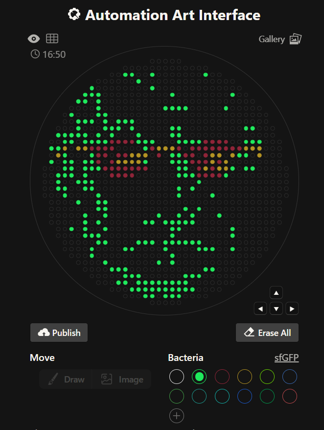
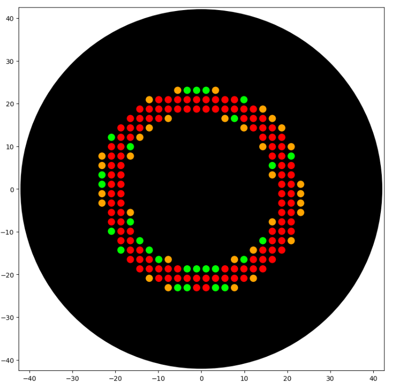
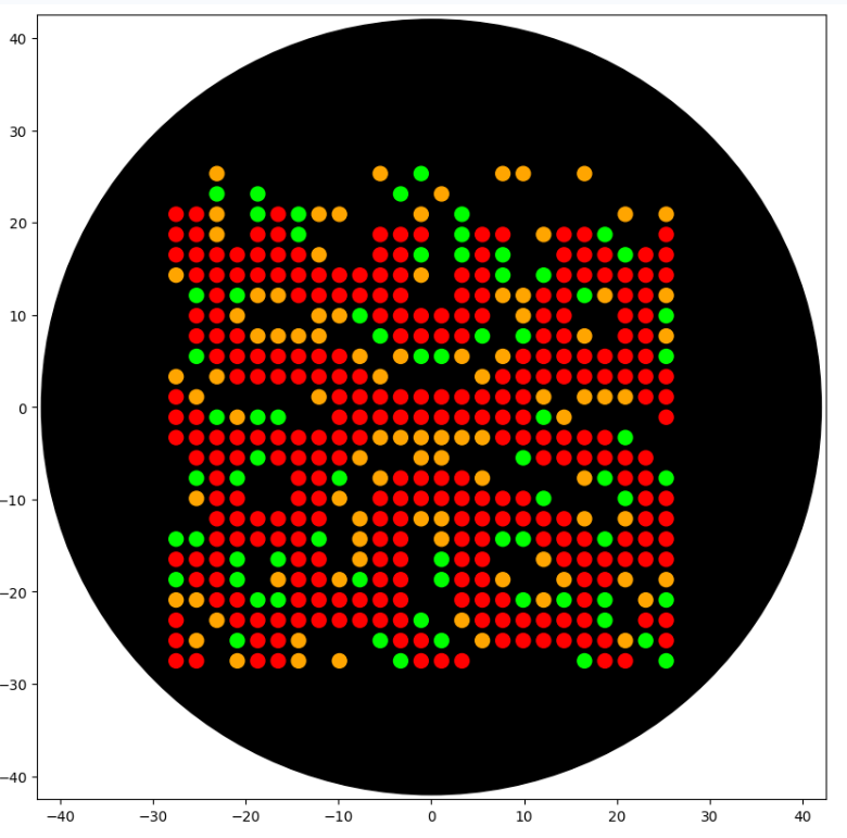
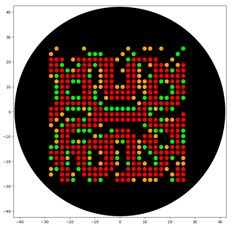
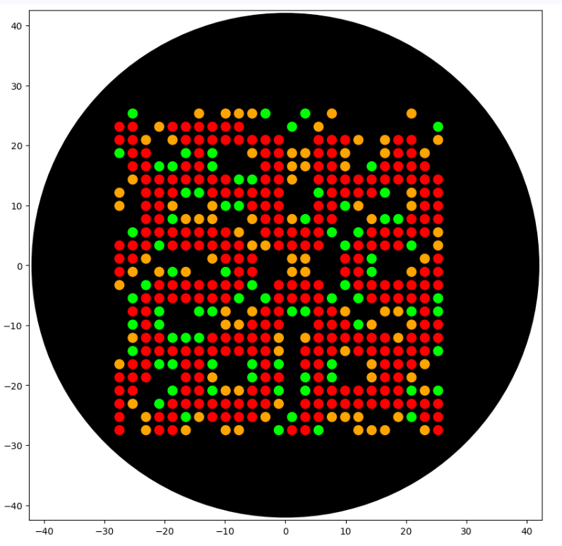
Precisely for this reason, in the context of this Opentrons experiment, I am interested in translating a dynamic of emergence into a very concrete material gesture — an image composed of discrete deposits, where a continuous phenomenon (reaction and diffusion) becomes a physical field of dots.
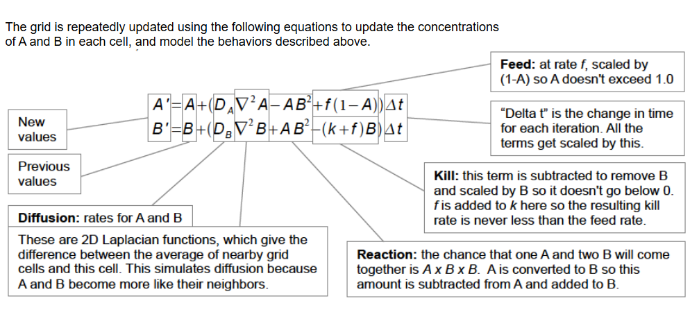
fromopentronsimporttypesimportsubprocess,sysimportnumpyasnpmetadata={# see https://docs.opentrons.com/v2/tutorial.html#tutorial-metadata'author':'Vivien','protocolName':'Gray-Scott Reaction-Diffusion Pattern','description':'Generates a reaction-diffusion pattern on an agar plate using the Gray-Scott model, pipetting where the B concentration is high.','source':'HTGAA 2026 Opentrons Lab','apiLevel':'2.20'}################################################################################# Gray-Scott Model Global Parameters and Functions############################################################################### Gray-Scott Model ParametersGS_DA=1.0GS_DB=0.5GS_F=0.014# Feed rate. Experiment with values like 0.035 (spots), 0.014 (worms), 0.062 (moving spots)GS_K=0.045# Kill rate. Experiment with values like 0.065 (spots), 0.045 (worms), 0.061 (moving spots)GS_DT=1.0#1. Mitosis / spots : f=0.0367, k=0.0649#2. Solitions / worms : f=0.030, k=0.062#3. Coral / dense : f=0.0545, k=0.062#4. Vibe : f = 0.029, K = 0.057#5. labyrythn : f = 0.060, K = 0.063deflaplace(Z):"""Weighted 3x3 Laplacian (Karl Sims style) using numpy.roll."""return(-1.0*Z+0.2*(np.roll(Z,1,axis=0)+np.roll(Z,-1,axis=0)+np.roll(Z,1,axis=1)+np.roll(Z,-1,axis=1))+0.05*(np.roll(np.roll(Z,1,axis=0),1,axis=1)+np.roll(np.roll(Z,1,axis=0),-1,axis=1)+np.roll(np.roll(Z,-1,axis=0),1,axis=1)+np.roll(np.roll(Z,-1,axis=0),-1,axis=1)))defsimulate_gray_scott(A,B,num_iterations):"""
Runs the Gray-Scott simulation for a given number of iterations.
Modifies A and B arrays in place.
"""for_inrange(num_iterations):lapA=laplace(A)lapB=laplace(B)reaction=A*B*BA+=(GS_DA*lapA-reaction+GS_F*(1-A))*GS_DTB+=(GS_DB*lapB+reaction-(GS_K+GS_F)*B)*GS_DTreturnA,B# Return A and B for clarity, though they are modified in-place################################################################################# Robot deck setup constants - don't change these##############################################################################TIP_RACK_DECK_SLOT=9COLORS_DECK_SLOT=6AGAR_DECK_SLOT=5PIPETTE_STARTING_TIP_WELL='A1'well_colors={'A1':'Red','B1':'Green','C1':'Orange'}defrun(protocol):################################################################################# Load labware, modules and pipettes############################################################################### Tipstips_20ul=protocol.load_labware('opentrons_96_tiprack_20ul',TIP_RACK_DECK_SLOT,'Opentrons 20uL Tips')# Pipettespipette_20ul=protocol.load_instrument("p20_single_gen2","right",[tips_20ul])# Modulestemperature_module=protocol.load_module('temperature module gen2',COLORS_DECK_SLOT)# Temperature Module Platetemperature_plate=temperature_module.load_labware('opentrons_96_aluminumblock_generic_pcr_strip_200ul','Cold Plate')# Choose where to take the colors fromcolor_plate=temperature_plate# Agar Plateagar_plate=protocol.load_labware('htgaa_agar_plate',AGAR_DECK_SLOT,'Agar Plate')## TA MUST CALIBRATE EACH PLATE!# Get the top-center of the plate, make sure the plate was calibrated before running thiscenter_location=agar_plate['A1'].top()pipette_20ul.starting_tip=tips_20ul.well(PIPETTE_STARTING_TIP_WELL)################################################################################# Patterning#################################################################################### Helper functions for this lab#### pass this e.g. 'Red' and get back a Location which can be passed to aspirate()deflocation_of_color(color_string):forwell,colorinwell_colors.items():ifcolor.lower()==color_string.lower():returncolor_plate[well]raiseValueError(f"No well found with color {color_string}")# For this lab, instead of calling pipette.dispense(1, loc) use this: dispense_and_detach(pipette, 1, loc)defdispense_and_detach(pipette,volume,location):"""
Move laterally 5mm above the plate (to avoid smearing a drop); then drop down to the plate,
dispense, move back up 5mm to detach drop, and stay high to be ready for next lateral move.
5mm because a 4uL drop is 2mm diameter; and a 2deg tilt in the agar pour is >3mm difference across a plate.
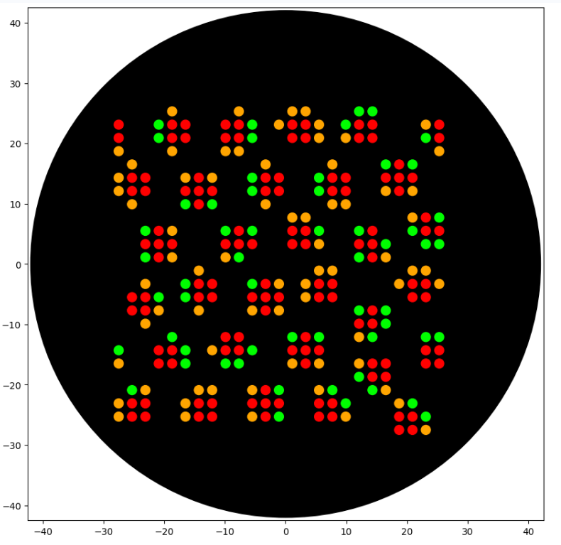
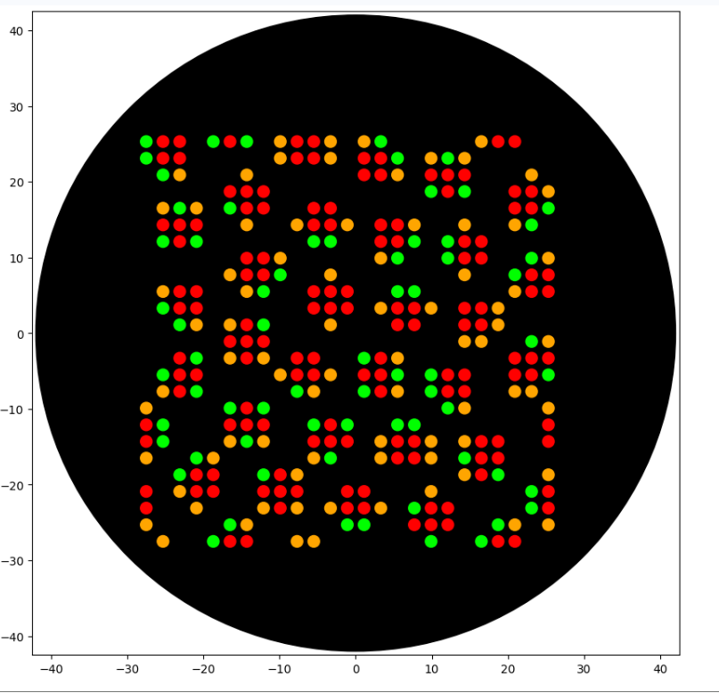
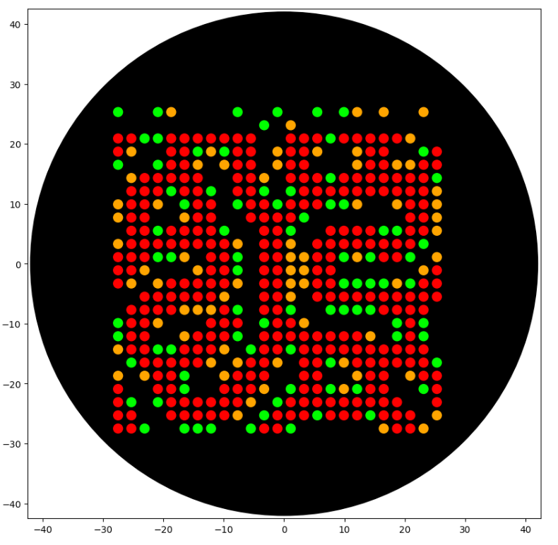
"""assert(isinstance(volume,(int,float)))above_location=location.move(types.Point(z=location.point.z+5))# 5mm abovepipette.move_to(above_location)# Go to 5mm above the dispensing locationpipette.dispense(volume,location)# Go straight downwards and dispensepipette.move_to(above_location)# Go straight up to detach drop and stay high###### YOUR CODE HERE to create your design (Gray-Scott Reaction-Diffusion Model)#### Grid size for simulationsize=100# Reduced size to make simulation faster and denser pattern on plateA=np.ones((size,size))B=np.zeros((size,size))# Create a central square seed for Br=5A[size//2-r:size//2+r,size//2-r:size//2+r]=0.5B[size//2-r:size//2+r,size//2-r:size//2+r]=0.25# Add small random noise to the entire grid to introduce variation# This helps break symmetry and encourages diverse pattern formationA+=np.random.rand(size,size)*0.05# Add noise up to 0.05B+=np.random.rand(size,size)*0.05# Add noise up to 0.05B_min=float(B.min());B_max=float(B.max());B_mean=float(B.mean())print("B stats:",B_min,B_mean,B_max)# Ensure values remain within bounds [0, 1] after adding noiseA=np.clip(A,0.0,1.0)B=np.clip(B,0.0,1.0)print("Running Gray-Scott simulation...")# Define the number of simulation iterations hereSIMULATION_ITERATIONS=8000# Initial run for 400 iterationsA,B=simulate_gray_scott(A,B,SIMULATION_ITERATIONS)print(f"Gray-Scott simulation complete after {SIMULATION_ITERATIONS} iterations. Starting patterning.")print(f"To run more iterations, change the 'SIMULATION_ITERATIONS' variable in the code and re-run this cell and the visualization cell below.")# Patterning Parameters for OpentronsPIPETTE_VOLUME=1# 1uL per dotASPIRATE_VOLUME=16# Aspirate up to this much at a timeMAX_DOTS_PER_COLOR=300# Maximum number of dots to dispense per color# Colors to use for B componentsCOLOR_FOR_PRIMARY_PATTERN='Green'# For the 'thick black lines' patternCOLOR_FOR_SECONDARY_PATTERN='Orange'# For other B concentrationsCOLOR_FOR_TERTIARY_PATTERN='Red'# For the highest B concentrations# Thresholds for B values# For 'thick black lines' (Green color)PRIMARY_PATTERN_B_LOWER_THRESHOLD=0.40*B_maxPRIMARY_PATTERN_B_UPPER_THRESHOLD=0.70*B_max# This value will also define the lower bound for Red# For the secondary pattern (Orange color)# This will catch 'B' values that are above this, but not in the primary or tertiary pattern bandsSECONDARY_PATTERN_B_THRESHOLD=0.20*B_max# Adjust this percentage as neededprint("Using Red Pattern (Highest B) threshold: B >=",PRIMARY_PATTERN_B_UPPER_THRESHOLD)print("Using Green Pattern (Mid B - 'thick lines') B thresholds: (",PRIMARY_PATTERN_B_LOWER_THRESHOLD,",",PRIMARY_PATTERN_B_UPPER_THRESHOLD,")")print("Using Orange Pattern (Lower B) threshold: (",SECONDARY_PATTERN_B_THRESHOLD,",",PRIMARY_PATTERN_B_LOWER_THRESHOLD,"]")# Agar plate dimensions (estimated for a standard 90mm round agar plate,# patterning in a 70x70mm square area roughly) to fit the patternPATTERN_AREA_WIDTH_MM=55# Reduced from 85mm to fit within 40mm radius safe areaPATTERN_AREA_HEIGHT_MM=55# Reduced from 85mm to fit within 40mm radius safe area# Calculate scaling factor to map grid coordinates to millimeters on the platescale_x=PATTERN_AREA_WIDTH_MM/sizescale_y=PATTERN_AREA_HEIGHT_MM/size# Add sampling step for clearer dotsSAMPLING_STEP=4# Pipette every Nth pixel to create distinct dotsDOT_SPACING_MM=SAMPLING_STEP*scale_x# Actual physical spacing between dot centersprint(f"Desired dot spacing for distinct patterns: {DOT_SPACING_MM:.2f} mm (approx. 2mm drop diameter).")pipetted_count_primary=0# Greenpipetted_count_secondary=0# Orangepipetted_count_tertiary=0# Red# --- Pipetting for Tertiary Pattern (Red component - highest B concentration) ---pipette_20ul.pick_up_tip()pipette_20ul.aspirate(ASPIRATE_VOLUME,location_of_color(COLOR_FOR_TERTIARY_PATTERN))current_pipette_volume=ASPIRATE_VOLUMEprint(f"Starting patterning for Tertiary Pattern with {COLOR_FOR_TERTIARY_PATTERN}.")foryinrange(0,size,SAMPLING_STEP):forxinrange(0,size,SAMPLING_STEP):ifB[y,x]>=PRIMARY_PATTERN_B_UPPER_THRESHOLD:ifcurrent_pipette_volume<PIPETTE_VOLUME:pipette_20ul.aspirate(ASPIRATE_VOLUME,location_of_color(COLOR_FOR_TERTIARY_PATTERN))current_pipette_volume+=ASPIRATE_VOLUMEx_offset_mm=(x-size/2)*scale_xy_offset_mm=(y-size/2)*scale_yadjusted_location=center_location.move(types.Point(x=x_offset_mm,y=y_offset_mm))dispense_and_detach(pipette_20ul,PIPETTE_VOLUME,adjusted_location)current_pipette_volume-=PIPETTE_VOLUMEpipetted_count_tertiary+=1ifpipetted_count_tertiary>=MAX_DOTS_PER_COLOR:breakifpipetted_count_tertiary>=MAX_DOTS_PER_COLOR:breakpipette_20ul.drop_tip()print(f"Total {pipetted_count_tertiary} drops pipetted for Tertiary Pattern using {COLOR_FOR_TERTIARY_PATTERN}.")# --- Pipetting for Primary Pattern (Green component - 'thick lines') ---pipette_20ul.pick_up_tip()pipette_20ul.aspirate(ASPIRATE_VOLUME,location_of_color(COLOR_FOR_PRIMARY_PATTERN))current_pipette_volume=ASPIRATE_VOLUMEprint(f"Starting patterning for Primary Pattern with {COLOR_FOR_PRIMARY_PATTERN}.")foryinrange(0,size,SAMPLING_STEP):forxinrange(0,size,SAMPLING_STEP):if(B[y,x]>PRIMARY_PATTERN_B_LOWER_THRESHOLD)and(B[y,x]<PRIMARY_PATTERN_B_UPPER_THRESHOLD):ifcurrent_pipette_volume<PIPETTE_VOLUME:pipette_20ul.aspirate(ASPIRATE_VOLUME,location_of_color(COLOR_FOR_PRIMARY_PATTERN))current_pipette_volume+=ASPIRATE_VOLUMEx_offset_mm=(x-size/2)*scale_xy_offset_mm=(y-size/2)*scale_yadjusted_location=center_location.move(types.Point(x=x_offset_mm,y=y_offset_mm))dispense_and_detach(pipette_20ul,PIPETTE_VOLUME,adjusted_location)current_pipette_volume-=PIPETTE_VOLUMEpipetted_count_primary+=1ifpipetted_count_primary>=MAX_DOTS_PER_COLOR:breakifpipetted_count_primary>=MAX_DOTS_PER_COLOR:breakpipette_20ul.drop_tip()print(f"Total {pipetted_count_primary} drops pipetted for Primary Pattern using {COLOR_FOR_PRIMARY_PATTERN}.")# --- Pipetting for Secondary Pattern (Orange component) ---pipette_20ul.pick_up_tip()pipette_20ul.aspirate(ASPIRATE_VOLUME,location_of_color(COLOR_FOR_SECONDARY_PATTERN))current_pipette_volume=ASPIRATE_VOLUMEprint(f"Starting patterning for Secondary Pattern with {COLOR_FOR_SECONDARY_PATTERN}.")foryinrange(0,size,SAMPLING_STEP):forxinrange(0,size,SAMPLING_STEP):# Dispense Orange if B is above its threshold, AND NOT in the Green or Red bandif(B[y,x]>SECONDARY_PATTERN_B_THRESHOLD)and(B[y,x]<=PRIMARY_PATTERN_B_LOWER_THRESHOLD):ifcurrent_pipette_volume<PIPETTE_VOLUME:pipette_20ul.aspirate(ASPIRATE_VOLUME,location_of_color(COLOR_FOR_SECONDARY_PATTERN))current_pipette_volume+=ASPIRATE_VOLUMEx_offset_mm=(x-size/2)*scale_xy_offset_mm=(y-size/2)*scale_yadjusted_location=center_location.move(types.Point(x=x_offset_mm,y=y_offset_mm))dispense_and_detach(pipette_20ul,PIPETTE_VOLUME,adjusted_location)current_pipette_volume-=PIPETTE_VOLUMEpipetted_count_secondary+=1ifpipetted_count_secondary>=MAX_DOTS_PER_COLOR:breakifpipetted_count_secondary>=MAX_DOTS_PER_COLOR:breakpipette_20ul.drop_tip()print(f"Total {pipetted_count_secondary} drops pipetted for Secondary Pattern using {COLOR_FOR_SECONDARY_PATTERN}.")
# Execute Simulation / Visualization -- don't change this code block
protocol = OpentronsMock(well_colors)
run(protocol)
protocol.visualize()

 B stats: 1.1769677182305039e-07 0.02738330028607403 0.2993330786497384
Running Gray-Scott simulation...
Gray-Scott simulation complete after 8000 iterations. Starting patterning.
To run more iterations, change the 'SIMULATION_ITERATIONS' variable in the code and re-run this cell and the visualization cell below.
Using Red Pattern (Highest B) threshold: B >= 0.20953315505481687
Using Green Pattern (Mid B - 'thick lines') B thresholds: ( 0.11973323145989537 , 0.20953315505481687 )
Using Orange Pattern (Lower B) threshold: ( 0.059866615729947684 , 0.11973323145989537 ]
Desired dot spacing for distinct patterns: 2.20 mm (approx. 2mm drop diameter).
Starting patterning for Tertiary Pattern with Red.
Total 0 drops pipetted for Tertiary Pattern using Red.
Starting patterning for Primary Pattern with Green.
Total 0 drops pipetted for Primary Pattern using Green.
Starting patterning for Secondary Pattern with Orange.
Total 0 drops pipetted for Secondary Pattern using Orange.

=== VOLUME TOTALS BY COLOR ===
	Orange:		 aspirated 16	 dispensed 0		##### WASTING BIO-INK : more aspirated than dispensed!
	Green:		 aspirated 16	 dispensed 0		##### WASTING BIO-INK : more aspirated than dispensed!
	Red:		 aspirated 16	 dispensed 0		##### WASTING BIO-INK : more aspirated than dispensed!
	[all colors]:	[aspirated 48]	[dispensed 0]

=== TIP COUNT ===
	 Used 3 tip(s)  (ideally exactly one per unique color)
```
I used Gemini (2.5) to help translate a Gray-Scott reaction–diffusion model into a stable Opentrons protocol and to choose a robust rendering strategy (iso-contour band → dot sampling) that produces reliable aesthetic output under time/volume constraints.
Post-Lab Questions
Find and describe a published paper that utilizes the Opentrons or an automation tool to achieve novel biological applications.
The paper does not focus only on Opentrons specifically, but it discusses how open hardware platforms — including OpenTrons — are transforming access to biological research tools. The author explains how open-source automation systems allow laboratories to build, adapt, and maintain their own equipment instead of relying only on expensive proprietary machines.
What is particularly interesting is the idea of “appropriate technology.” The paper argues that automation is not just about saving money. It is about local fabrication, adaptability, transparency, and knowledge transfer. Open systems such as OpenTrons make automation accessible to more researchers, especially in low-resource environments, while still enabling advanced biological workflows.
This approach supports reproducibility, customization, and global collaboration. Instead of being locked into closed commercial systems, researchers can modify and improve their automation tools to fit specific experimental needs.
In that sense, laboratory automation becomes not only a productivity tool, but also a platform for scientific autonomy and innovation.
Write a description about what you intend to do with automation tools for your final project.
Automation as a Tool to Explore the Behavioral Landscape of Living Materials
Automation tools such as Opentrons have been widely used for:
High-throughput DNA assembly
CRISPR editing workflows
Combinatorial genetic library screening
Automated protein expression testing
These systems increase reproducibility, reduce human variability, and enable scalable experimentation. In most cases, automation serves to optimize molecular workflows and accelerate genetic engineering cycles.
However, my interest in automation is different.
Moving Beyond Optimization
In classical bioprocess engineering, automation is used to:
Optimize growth conditions
Reduce experimental noise
Standardize reproducibility
Improve yield
But living materials — such as bacterial cellulose biofilms — do not behave like linear industrial systems.
They exhibit:
Non-linear responses
Narrow stability windows
Emergent morphologies
Phase transitions under small parameter shifts
Traditional experimental design (e.g., Taguchi matrices) assumes relatively smooth and predictable response surfaces. In living systems, this assumption often fails. Small changes in pH, oxygen availability, carbon source, or metal ions can lead to abrupt structural transitions.
Automation, in this context, is not merely an efficiency tool.
It becomes a way to systematically explore instability and emergence.
My Intended Use of Automation
1. Mapping Morphogenetic Regimes of Bacterial Cellulose
Instead of optimizing for maximum growth, I aim to use automation to:
The objective is to map how living cellulose changes:
Thickness
Porosity
Impedance
Mechanical anisotropy
Conductive behavior
This transforms automation into a cartographic tool:
Not optimizing yield, but mapping the behavioral topology of a living material.
2. Spatial Programming of Living Matter
A more ambitious direction is to use liquid handling automation to:
Deposit gradients of dopants
Create patterned functional zones
Introduce local conductivity modulation
Encode anisotropy into growing pellicles
Instead of post-processing materials (e.g., adding graphene or PEDOT in situ), this approach attempts to let functionality emerge during growth.
Automation allows spatial control.
Living matter performs the structuration.
3. Toward a Cybernetic Living Material System
A future extension would integrate measurement and feedback:
Grow bacterial cellulose
Measure impedance or electrical response
Adjust copper or nutrient concentration automatically
Iterate
This creates a cybernetic loop:
Living material → Measurement → Algorithmic adjustment → Modified growth
Automation becomes a mediator between biological behavior and computational control.
Why This Matters
This project shifts the role of automation from:
Eliminating biological variability to:
Engaging systematically with biological variability.
Rather than forcing the living system into industrial predictability, automation is used to:
Detect bifurcations
Explore phase transitions
Reveal hidden regimes
Enable programmable morphogenesis
In this sense, automation becomes a bridge between:
Synthetic biology
Biofabrication
Morphogenesis
Cybernetic design
It allows living matter to be explored not as a static substrate, but as a dynamic, programmable system.