Week 10 HW: Advanced Imaging & Measurement Technology
Table of Contents
Homework: Waters Part III — Peptide Mapping - Primary Structure
- Lysine (K) and Arginine (R) Count in eGFP
- eGFP Sequence with K and R Highlighted
- Expected Number of Tryptic Peptides from eGFP
- Number of Chromatographic Peaks in the eGFP Peptide Map
- Comparison Between Experimental Peaks and Predicted Peptides
- Peptide m/z, Charge State, and Singly Charged Mass
- Peptide Identification and Mass Accuracy
- Percentage of Sequence Confirmed by Peptide Mapping
Homework: Final Project
## Final Project — Measurement Plan
My final project is:
Growable Impedance-Sensitive Surface from Bacterial Cellulose via Tyr1-Mediated Eumelanin
The goal is to engineer or design a bacterial cellulose material whose electrochemical behavior is modified through Tyr1-mediated eumelanin production.
1. Genetic Construct Verification
I would first measure whether the tyr1 expression cassette was correctly assembled.
What I want to measure:
- presence of the
tyr1gene, - correct promoter/RBS/CDS/terminator structure,
- correct plasmid size,
- absence of major cloning errors.
Technologies:
- PCR / colony PCR,
- agarose gel electrophoresis,
- Sanger sequencing.
Expected result: A correct PCR band at the expected size, followed by sequencing confirming that the tyr1 coding sequence and regulatory elements are intact.
2. Tyr1 Protein Expression
I would measure whether the transformed bacteria actually express Tyr1.
What I want to measure:
- presence of Tyr1 protein,
- approximate protein size,
- expression level.
Technologies:
- SDS-PAGE,
- optional Western blot if a His-tag or antibody is available.
Expected result: A protein band corresponding to Tyr1, around the expected molecular weight for tyrosinase.
3. Melanin Production
The central functional readout is whether Tyr1 produces eumelanin.
What I want to measure:
- visible pigmentation,
- melanin intensity,
- spatial distribution of pigmentation in the bacterial cellulose pellicle.
Technologies:
- photography under controlled lighting,
- image analysis,
- UV-Vis spectroscopy,
- optional colorimetric quantification.
Expected result: The cellulose pellicle should progressively darken when exposed to L-tyrosine and copper under suitable pH conditions.
4. Bacterial Cellulose Growth
Because the material itself is grown, I would measure bacterial cellulose production.
What I want to measure:
- wet mass,
- dry mass,
- thickness,
- surface area,
- growth time,
- morphology.
Technologies:
- scale for mass,
- calipers or microscopy for thickness,
- photographic documentation,
- drying protocol for dry mass.
Expected result: A measurable pellicle that can be compared between wild-type and Tyr1-functionalized conditions.
5. Electrochemical / Impedance Behavior
This is the key material measurement.
What I want to measure:
- impedance magnitude,
- phase response,
- frequency-dependent behavior,
- hydration sensitivity,
- pressure/touch sensitivity,
- difference between native BC and melanin-rich BC.
Technologies:
- two-electrode or four-electrode setup,
- frequency sweep,
- controlled hydration measurements.
Expected result: Eumelanin-functionalized bacterial cellulose may show altered impedance behavior compared to native bacterial cellulose, especially under different hydration or ionic conditions.
6. Environmental / Culture Conditions
Because cellulose growth and melanin production depend strongly on the culture environment, I would also monitor:
What I want to measure:
- pH,
- sugar consumption,
- conductivity of the medium,
- hydration state,
- incubation time.
Technologies:
- pH meter or pH strips,
- conductivity meter,
- refractometer or glucose assay,
- mass-based hydration tracking.
Expected result: These measurements help connect metabolic state with material formation and final impedance behavior.
Summary Table
| Measurement | Purpose | Technology |
|---|---|---|
| tyr1 DNA presence | Confirm construct | PCR, gel electrophoresis |
| Sequence correctness | Confirm cassette integrity | Sanger sequencing |
| Tyr1 expression | Confirm protein production | SDS-PAGE / Western blot |
| Melanin production | Confirm functional enzyme activity | Photography, UV-Vis |
| BC growth | Quantify material formation | Mass, thickness, imaging |
| Impedance | Measure functional material behavior | LCR meter / impedance analyzer |
| pH / conductivity | Monitor culture state | pH meter, conductivity meter |
Overall Goal
The final objective is to connect:
This measurement plan would allow me to evaluate not only whether the genetic system works, but also whether the biological modification produces a meaningful change in the material’s electrochemical properties.
Homework: Waters Part I — Molecular Weight
Waters Part I — eGFP Molecular Weight
Using the eGFP amino acid sequence provided in the assignment, including:
- the
LElinker, - and the C-terminal
6xHispurification tag (HHHHHH),
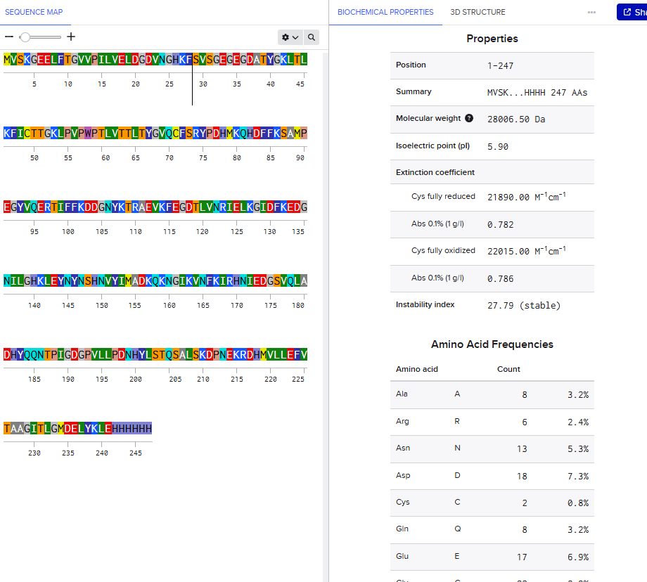
I calculated the theoretical molecular weight and isoelectric point using the ExPASy Compute pI/Mw tool.
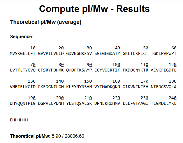
Results
| Property | Value |
|---|---|
| Theoretical pI | 5.90 |
| Theoretical Molecular Weight | 28,006.60 Da |
| Approximate Molecular Weight | 28.0 kDa |
Because LC-MS intact protein analysis is performed under denaturing solvent conditions, I would expect eGFP to unfold and produce a charge-state distribution corresponding to the denatured protein around ~28 kDa after deconvolution.
The His-tag and linker slightly increase the final molecular weight compared to native GFP.
2. Molecular Weight from Adjacent Charge States
From Figure 1, I selected two adjacent charge-state peaks:
| Peak | m/z |
|---|---|
| z + 1 peak | 875.4421 |
| z peak | 903.7138 |
Using the adjacent charge-state equation, the estimated charge state is:
Then the molecular weight can be calculated from:
MW = z × (m/z - H⁺)
where:
H⁺ = 1.0073 Da
So:
MW = 31 × (903.7138 - 1.0073) MW ≈ 27,983.9 Da Comparison with theoretical mass
The theoretical molecular weight calculated from the eGFP sequence was:
MW_theory = 28,006.60 Da
The accuracy/error is:
|27,983.9 - 28,006.6| / 28,006.6 = 0.00081
or approximately:
0.081% Interpretation
The molecular weight estimated from the adjacent charge states is very close to the theoretical eGFP molecular weight. Small differences may come from peak reading precision, isotope distribution, adducts, or calibration differences in the LC-MS measurement.
Charge State Observation from the Zoomed-In Peak
Yes, the charge state can be observed from the zoomed-in isotopic peak distribution.
In the inset spectrum, the individual isotope peaks are separated by approximately:
For multiply charged ions in mass spectrometry:
Charge state z ≈ 1 / Δ(m/z)
So:
z ≈ 1 / 0.032 ≈ 31
This corresponds well to the charge state estimated previously from the adjacent peak method.
The reason this works is that highly charged proteins produce isotope peaks that are very closely spaced in m/z space. The spacing between isotopic peaks becomes inversely proportional to the charge state.
Homework: Waters Part II — Secondary/Tertiary structure
Native vs Denatured Protein Conformations
Proteins can exist in either a native folded state or a denatured unfolded state.
In the native state, the protein maintains its compact three-dimensional structure through:
- hydrogen bonding,
- hydrophobic interactions,
- electrostatic interactions,
- and sometimes disulfide bonds.
When a protein denatures, these stabilizing interactions are disrupted. The protein unfolds and exposes amino acid residues that were previously buried inside the structure. In mass spectrometry, denaturation is commonly induced using acidic solvents and organic solvents such as acetonitrile.
This unfolding strongly affects the protein charge-state distribution during electrospray ionization (ESI). A folded protein has a compact surface with fewer solvent-accessible protonation sites, so it acquires fewer charges. An unfolded protein exposes many more basic residues to the solvent, allowing it to acquire many additional protons.
As a result:
Native proteins usually produce:
- lower charge states,
- higher m/z peaks,
- narrower charge-state distributions.
Denatured proteins usually produce:
- higher charge states,
- lower m/z peaks,
- broader charge-state distributions.
Interpretation of Figure 2
In the native eGFP spectrum (bottom/red spectrum), the peaks appear at much higher m/z values (~2500–2800 m/z), indicating that the protein carries relatively few charges. This is consistent with a compact folded structure.
In the denatured eGFP spectrum (top/green spectrum), the peaks shift toward lower m/z values (~700–1400 m/z) and show a much broader charge-state distribution. This indicates that the protein has unfolded and acquired many more charges during ionization.
Therefore, the mass spectrometer indirectly detects protein folding state through the observed charge-state distribution:
- compact folded proteins → low charge states,
- unfolded proteins → high charge states.
Charge State of the Native eGFP Peak at ~2800 m/z
Yes, the charge state of the native eGFP peak around ~2800 m/z can be determined from the isotopic peak spacing in the zoomed-in spectrum.
The isotope peaks are separated by approximately:
In electrospray ionization mass spectrometry, the relationship between isotope spacing and charge state is:
z ≈ 1 / Δ(m/z)
Therefore:
z ≈ 1 / 0.09 ≈ 11
So the peak near ~2800 m/z corresponds approximately to the:
11+ charge state
This makes sense for native folded eGFP because folded proteins generally acquire fewer charges than denatured proteins. The compact native structure exposes fewer protonatable residues, resulting in lower charge states and therefore higher m/z values.
Homework: Waters Part III — Peptide Mapping - primary structure
Lysine (K) and Arginine (R) Count in eGFP
Trypsin cleaves peptide bonds after:
- Lysine (K)
- Arginine (R)
(except when followed by Proline).
Using the eGFP sequence provided, I counted:
| Amino Acid | Count |
|---|---|
| Lysine (K) | 20 |
| Arginine (R) | 6 |
| Total tryptic cleavage residues | 26 |
eGFP Sequence with K and R Highlighted
The high number of Lysine and Arginine residues explains why trypsin digestion generates many smaller peptides suitable for LC-MS peptide mapping.
Expected Number of Tryptic Peptides from eGFP
Using the ExPASy PeptideMass tool with the parameters shown:
- Enzyme: Trypsin
- Missed cleavages: 0
- Monoisotopic masses
- Reduced cysteines
- Display peptides larger than 500 Da
the digestion of eGFP produced:
As shown in the PeptideMass output, this corresponds to approximately:
90.7% sequence coverage
The peptides listed correspond to the fragments expected after trypsin cleavage at Lysine (K) and Arginine (R) residues.

Number of Chromatographic Peaks in the eGFP Peptide Map
Using Figure 5a and counting chromatographic peaks between:
with approximately:
10% relative abundance
I observe approximately:
20 major chromatographic peaks
These peaks correspond to different tryptic peptides generated from the digestion of eGFP. Each peptide elutes at a different retention time depending on properties such as:
hydrophobicity, peptide length, charge, and amino acid composition.
The large number of peaks reflects the complexity of the peptide mixture produced after trypsin digestion.
The number of chromatographic peaks is close to, but slightly higher than, the number of peptides predicted by ExPASy.
ExPASy predicted:
From the chromatogram, I counted approximately:
20 major peaks between 0.5 and 6 minutes
So there appear to be slightly more chromatographic peaks than predicted peptides.
This difference is expected because one theoretical peptide can sometimes appear as more than one chromatographic signal due to different charge states, oxidation states, adducts, missed cleavages, or partially resolved co-eluting species. Also, not every chromatographic peak necessarily corresponds to a unique eGFP tryptic peptide.
Peptide m/z, Charge State, and Singly Charged Mass
From Figure 5b, the most abundant peptide peak is at: m/z = 525.767 In the zoomed-in isotope distribution, the isotope peaks are separated by approximately: 526.259 - 525.767 = 0.492
Since isotope spacing is approximately: 1 / z the charge state is: z ≈ 1 / 0.492 ≈ 2 So the peptide is mainly observed as a: 2+ ion To calculate the singly charged peptide mass:[M+H]+ = (m/z × z) - (z - 1) × H+
Using:
This matches the singly charged peak observed near: m/z ≈ 1050.52
Peptide Identification and Mass Accuracy
From Question 5, the experimentally measured singly charged peptide mass was: MW_experimental ≈ 1050.52 Da Comparing this value with the predicted tryptic peptide masses from the ExPASy PeptideMass output, the closest match is:
Therefore, the peptide observed at retention time 2.78 min is most likely:
Using: Accuracy = |MW_experimental - MW_theory| / MW_theory and converting to ppm: ppm error = Accuracy × 10^6
Using: MW_experimental = 1050.5238 MW_theory = 1050.5214 ppm error = (|1050.5238 - 1050.5214| / 1050.5214) × 10^6 ppm error ≈ 2.3 ppm Interpretation
A mass error of only a few ppm indicates excellent agreement between the experimental LC-MS measurement and the theoretical peptide mass prediction.
Percentage of Sequence Confirmed by Peptide Mapping
Based on Figure 6, the LC-MS peptide mapping identified: 88% sequence coverage
This means that peptides corresponding to approximately 88% of the eGFP amino acid sequence were experimentally detected and confirmed by LC-MS/MS analysis.
The uncovered regions likely correspond to:
peptides that are too small, poorly ionized, difficult to separate chromatographically, or outside the optimal mass detection range.
Homework: Waters Part IV — Oligomers
KLH Oligomeric State Assignment from CDMS
Using the subunit masses:
| Subunit | Mass |
|---|---|
| 7FU | 340 kDa |
| 8FU | 400 kDa |
we can calculate the expected oligomer masses.
Calculations
7FU Decamer 10 × 340 kDa = 3400 kDa = 3.4 MDa This corresponds to the peak near: 3.4 MDa
8FU Didecamer A didecamer contains 20 subunits: 20 × 400 kDa = 8000 kDa = 8.0 MDa This corresponds to the large peak near: 8.33 MDa
8FU 3-Decamer A 3-decamer contains 30 subunits: 30 × 400 kDa = 12000 kDa = 12.0 MDa This corresponds to the peak near: 12.67 MDa
8FU 4-Decamer A 4-decamer contains 40 subunits: 40 × 400 kDa = 16000 kDa = 16.0 MDa This corresponds to the lower-intensity signal around: 16 MDa
Summary Table
| Species | Calculation | Expected Mass | Observed Peak |
|---|---|---|---|
| 7FU Decamer | 10 × 340 kDa | 3.4 MDa | ~3.4 MDa |
| 8FU Didecamer | 20 × 400 kDa | 8.0 MDa | ~8.33 MDa |
| 8FU 3-Decamer | 30 × 400 kDa | 12.0 MDa | ~12.67 MDa |
| 8FU 4-Decamer | 40 × 400 kDa | 16.0 MDa | ~16 MDa |