🌿 Hi, I’m Yutong — Wellesley College ‘26 with background in Computational Cognitive Science & Biological Sciences
🔬 Scientist · 📸 Wildlife Photographer · 🎼 Guzheng Musician I aspire to be a design engineer in wearable health technology and smart pet technology. I believe nature is the best designer and want to build tools that listen to bodies, human and furry.
🗣️ Languages: Suzhou dialect, Mandarin, English, German · dabbled in Spanish and Hindi
🐾 how i got here
I took my first bio class in Organismal Biology in freshman fall, thinking it would be my last.
Spoiler: it wasn’t.
I couldn’t stop signing up for more animal-related bio classes, and somehow that snowballed into fieldwork across three continents.
🌏 where i’ve worked
🏔️ June 2023 · Sanjiangyuan, China — Animal conservation with the Sanjiangyuan Qumalai Ecological Protection & Wildlife Monitoring Association (中国三江源曲麻莱生态保护野生生物监测协会).
🐢 May 2024 · Little Cayman Island — Field research with my Tropical Ecology class on microplastics on epiphytes on seagrass — tiny pollutants, on tiny plants, on bigger plants.
🐒 January 2026 · Isla de los Monos, Iquitos, Peru — Volunteered at a monkey shelter deep in the rainforest. Had the best time hanging out with capuchins (Cebus), howler monkeys (Alouatta), saki monkeys (Pithecia), woolly monkeys (Lagothrix), titi monkeys (Plecturocebus), and tamarins (Saguinus). Survived without putting on any insect repellent.
💡 two things four years taught me
1. I love animals — ALIVE.
I can’t do any experiment that involves keeping vertebrates in captivity for experiments. Full stop.
The paper that keeps me studying bio is this one on the elephant facial motor system — sharing it here because it’s the kind of work that makes me believe in the field.
2. I need my hands in the work.
200% dry lab is not for me. I need to do things — dissect, build, pipette, troubleshoot, get my gloves dirty.
🧬 so… why HTGAA?
That’s exactly why I’m here — exploring more fun bio technologies, and looking for the sweet spot between rigorous science, hands-on tinkering, and the animals (and ideas) I love.
Project: Physarum-on-a-Chip Environmental Sensor The tool I want to develop is a Physarum-on-a-Chip environmental sensor – a microfluidic device that confines the plasmodium of Physarum polycephalum (slime mold!!) within a controlled chemotactic gradient array, and reads out the organism’s foraging behavior as a chemical-environment signal.
Why Physarum Physarum is a single multinucleated cell that solves problems no single cell “should” be able to solve. With no neurons and no central controller, it:
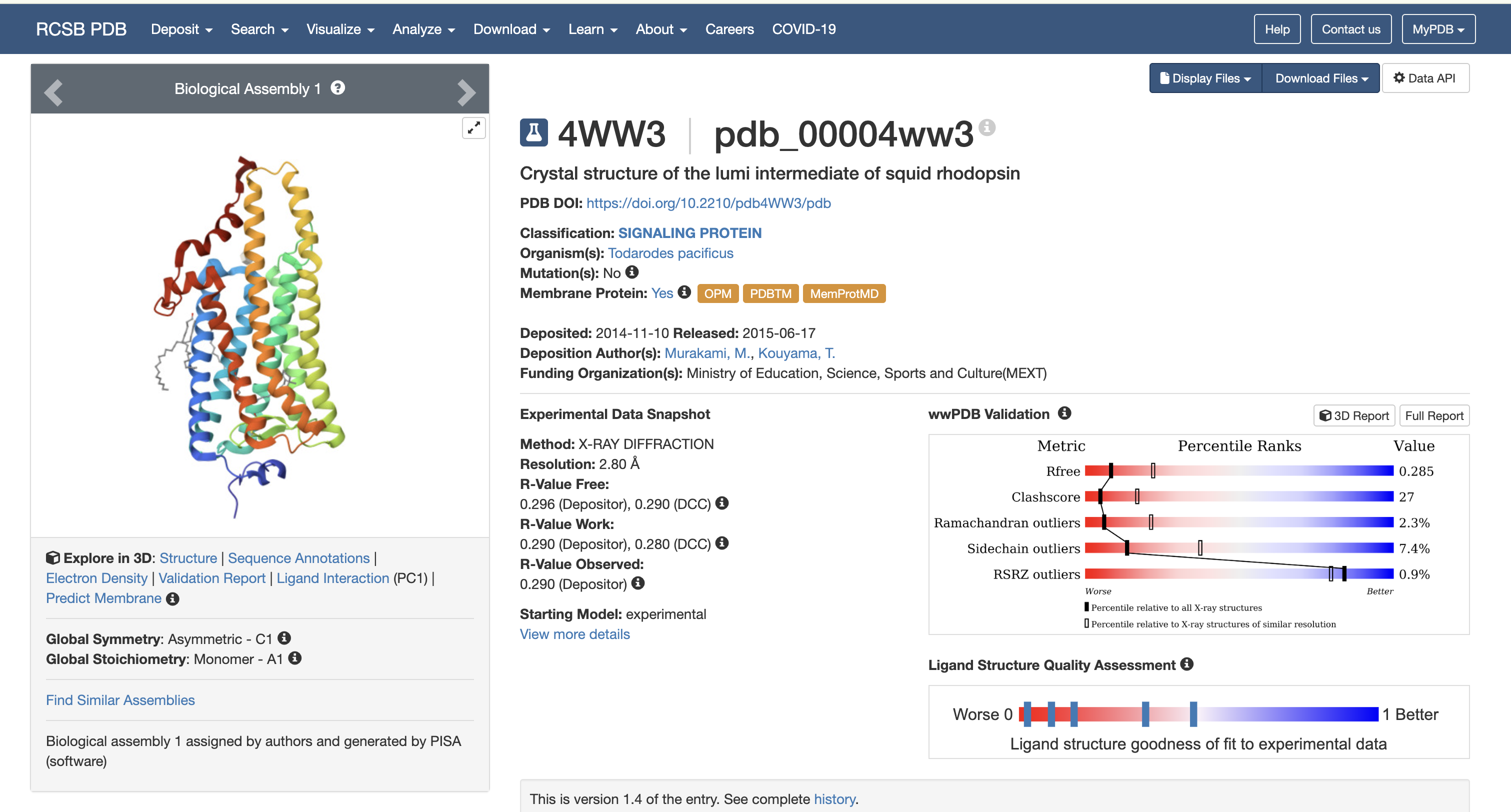
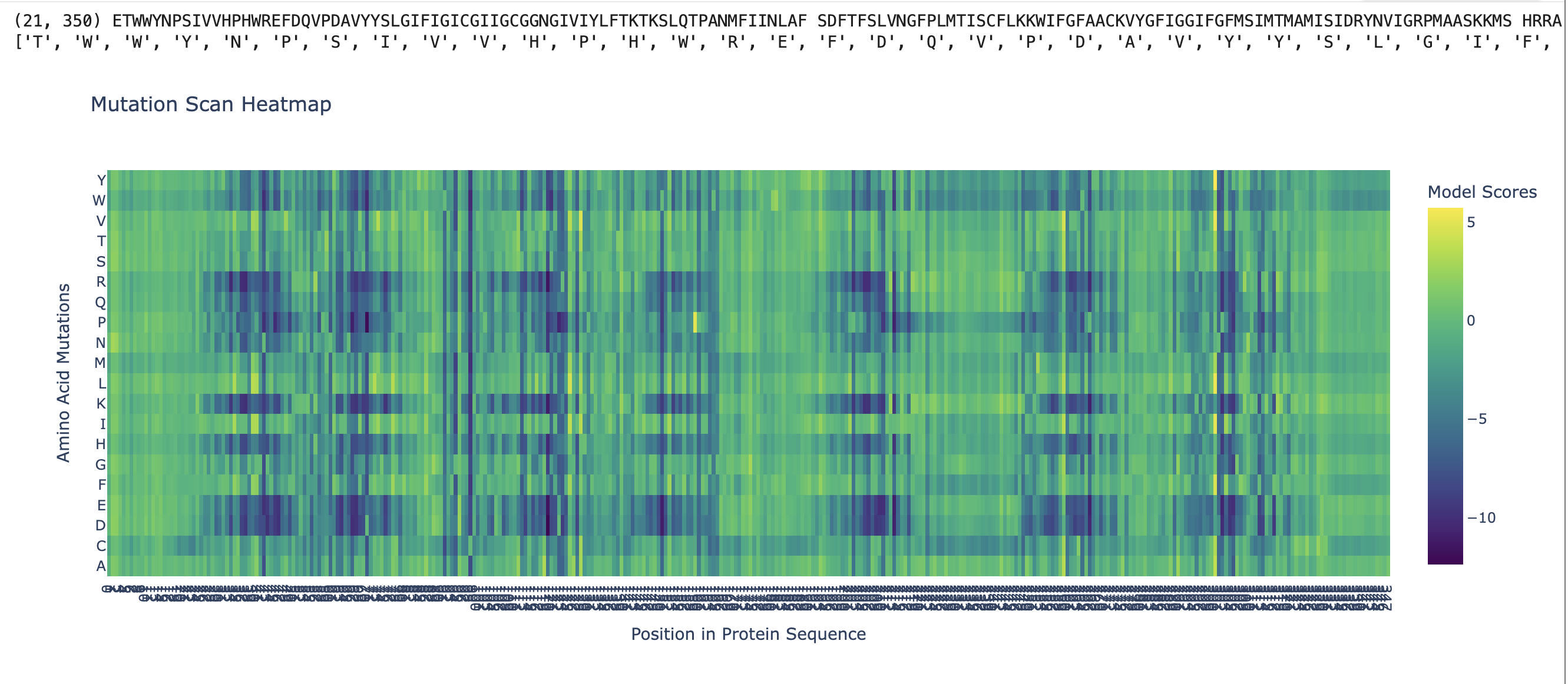
My protein this week is rhodopsin (RHO, UniProt P08100) Iti is a photon-sensing G-protein-coupled receptor in rod cells of the retina. As someone who works professionally in photography, this protein is basically my biological counterpart: a single 11-cis-retinal molecule sits in the middle of a 7-transmembrane GPCR and isomerizes to all-trans on absorbing one photon, triggering the entire phototransduction cascade. It is the sensor in the world’s oldest and most refined camera.
Published Paper Using Opentrons for a Novel Biological Application Paper: Bryant, J. A., Kellinger, M., Longmire, C., Miller, R., & Wright, R. C. (2023). AssemblyTron: flexible automation of DNA assembly with Opentrons OT-2 lab robots. Synthetic Biology, 8(1), ysac032. https://doi.org/10.1093/synbio/ysac032
What they built AssemblyTron is an open-source Python package that turns the ~$10k Opentrons OT-2 (with a thermocycler module) into a hands-free DNA-assembly workstation. It plugs into existing assembly-design tools (j5, Cello, Benchling) and executes the resulting build plans directly on the robot, covering three of the most common synbio assembly chemistries:
Part A — Conceptual Questions 1. How many molecules of amino acids are in 500 g of meat? Assume meat is roughly 20% protein by weight. The mass of protein is:
500 × 0.20 = 100 grams of protein.
Let’s assume the average molecular weight of a protein is 100 g/mol. Therefore:
Part 1: Generate Binders with PepMLM The original sequence of SOD1 is:
MATKAVCVLKGDGPVQGIINFEQKESNGPVKVWGSIKGLTEGLHGFHVHEFGDNTAGCTSAGPHFNPLSRKHGGPKDEERHVGDLGNVTADKDGVADVSIEDSVISLSGDHCIIGRTLVVHEKADDLGKGGNEESTKTGNAGSRLACGVIGIAQ Mutate the 4th amino acid A to V (A4V):
MATKVVCVLKGDGPVQGIINFEQKESNGPVKVWGSIKGLTEGLHGFHVHEFGDNTAGCTSAGPHFNPLSRKHGGPKDEERHVGDLGNVTADKDGVADVSIEDSVISLSGDHCIIGRTLVVHEKADDLGKGGNEESTKTGNAGSRLACGVIGIAQ Generate four peptides of length 12 amino acids conditioned on the mutant SOD1 sequence:
index Binder Pseudo Perplexity 0 HLYYAVALELKX 13.299815648347872 1 WRSYAVVLELWK 17.97100111129112 2 WRYYPVAAAWKK 11.081842724779028 3 WHYGAVGLRHKX 13.983770011694478 Part 2: Evaluate Binders with AlphaFold3 We submitted each peptide paired with the mutant SOD1 (A4V) sequence to the AlphaFold Server as separate chains to model the protein–peptide complex. All runs used seed 2026616022 for reproducibility.
Part 1. Questions 1. Phusion High-Fidelity PCR Master Mix Components Phusion DNA Polymerase — high-fidelity polymerase with 3′→5′ proofreading exonuclease activity; ~50× lower error rate than Taq dNTPs — nucleotide building blocks (dATP, dCTP, dGTP, dTTP) incorporated during strand synthesis HF Buffer + Mg²⁺ — provides optimal pH and ionic conditions; Mg²⁺ is an essential cofactor for polymerase activity Stabilizers — maintain enzyme activity during storage and reaction setup 2. Factors That Determine Primer Annealing Temperature GC content — G·C pairs have 3 H-bonds vs. 2 for A·T, raising T_m Primer length — longer primers = higher T_m Salt/Mg²⁺ concentration — stabilizes duplexes, increases T_m Primer secondary structure — hairpins or self-dimers reduce effective T_m Polymerase used — Phusion tolerates higher T_a than Taq; use NEB Tm Calculator for Phusion Rule of thumb: T_a ≈ T_m of the lower-melting primer (for Phusion)
Part 1. Intracellular Artificial Neural Networks Q1. Advantages of IANNs over Traditional Boolean Genetic Circuits A traditional genetic circuit works like a panel of on‑off light switches. Each gene is either fully expressed or completely silent, and the circuit’s output is a strict Boolean function of those binary inputs. An IANN, by contrast, behaves more like a set of dimmer switches connected through a mixing board. Each input can take any value within a continuous range, the connections have adjustable weights, and the final output is a smooth, graded signal instead of a hard 0 or 1.
##Part 1 1.Advantages of Cell-Free Over In Vivo Expression Cell-free protein synthesis (CFPS) removes the cell as a “black box” and allows you directly control and observe every variable in real time: pH, redox potential, ionic strength, and cofactor concentration.
2.Main Components and Their Roles
Component Role Cell extract Provides ribosomes, tRNA, synthetases, chaperones, and machinery DNA/mRNA template Encodes the target protein (plasmid or linear) RNA polymerase Transcribes DNA → mRNA (T7 RNAP is most common) Amino acids Raw building blocks for translation Energy system Supplies and recycles ATP/GTP to power translation Salts and buffer Maintains pH (~7.5) and ionic strength (Mg²⁺, K⁺ critical) Additives Chaperones, detergents, etc., added based on target needs 3.Energy Provision and ATP Regeneration
What to measure: Identity, mass, purity, and post-translational modifications of the target protein; concentration of a biomarker; oligomeric state.
How:
Intact mass by LC-MS (QTof) → confirms overall MW and detects unexpected modifications. Peptide mapping by tryptic digest + LC-MS/MS → confirms primary sequence and identifies PTM sites. Native MS / CDMS → reveals folded state and oligomeric assembly. SDS-PAGE / Western blot → quick purity and identity check before MS. UV-Vis (A280) → concentration. Part I — Molecular Weight of Intact eGFP Q1. Theoretical MW from sequence Sequence length: 247 residues (includes LE linker + HHHHHH His-tag).
Unfortunately I was away at CHI 2026 during the contribution window, so I didn’t get to commit a pixel in time.
Part B – Cell-Free Protein Synthesis B1. Role of each component E. coli Lysate
BL21 (DE3) Star Lysate (with T7 RNAP): The “factory floor” – a crude cytoplasmic extract carrying ribosomes, tRNAs, aminoacyl-tRNA synthetases, translation factors, and the T7 RNA polymerase needed to transcribe T7-promoter templates. The DE3 Star background also lacks RNase E activity, so mRNAs last longer. Salts / Buffer
Subsections of Homework
Week 1 HW: Principles & Practices
Project: Physarum-on-a-Chip Environmental Sensor
The tool I want to develop is a Physarum-on-a-Chip environmental sensor – a microfluidic device that confines the plasmodium of Physarum polycephalum (slime mold!!) within a controlled chemotactic gradient array, and reads out the organism’s foraging behavior as a chemical-environment signal.
Why Physarum
Physarum is a single multinucleated cell that solves problems no single cell “should” be able to solve. With no neurons and no central controller, it:
Finds shortest paths through mazes between food sources (Nakagaki et al., Nature, 2000).
Recapitulates the Tokyo rail network when offered food at the cities surrounding Tokyo (Tero et al., Science, 2010).
Remembers where it has been. Even without a nervous system, it lays down a trail of extracellular slime and avoids re-exploring already-visited areas. Reid et al. (PNAS, 2012) showed this functions as a kind of externalized spatial memory – the organism offloads its memory into the environment.
Anticipates periodic stimuli. Saigusa et al. (Phys. Rev. Lett., 2008) showed Physarum slows down in anticipation of regular cold pulses, then re-anticipates after the stimulus stops – a form of habituated learning without synapses.
This is bio-intelligence without a brain. The intracellular pathways are doing the work: oscillating cytoplasmic streaming, calcium waves, actomyosin contractions, and reaction-diffusion dynamics in the cell. The whole organism is a wet, living analog computer.
What I want to build
A device with these layers:
A microfluidic chip with PDMS channels patterned as a 2D array of “chambers” connected by narrow passages. Each chamber can be loaded with a chemoattractant (oat flake extract, glucose) or a chemorepellent (light, salt, quinine, or a target environmental contaminant – heavy metals, pesticide residue, microplastic extract).
A Physarum plasmodium introduced at a central inoculation chamber. It explores the array, makes routing decisions, and lays down its slime trail.
A camera + time-lapse readout that records the network topology over hours. Image analysis converts the plasmodium’s tube network into a graph – nodes, edges, weights.
A signal interpretation layer. The pattern of which chambers Physarum colonizes, which it avoids, and how fast it gets there encodes information about the chemical environment. A trained Physarum (one that has previously encountered a contaminant and “learned” to avoid it) gives a different network than a naive one.
Why I find this exciting
Three reasons:
The memory question. How does an organism without neurons remember a route? The extracellular slime hypothesis is elegant but probably not the whole story; intracellular calcium oscillations and tube-diameter hysteresis also encode state. Building a controlled platform lets me actually test which mechanism dominates in different conditions.
Bio-intelligence as an alternative paradigm. Most “intelligence” we build is digital and silicon. Physarum is a counter-example – distributed, analog, embodied, and runs on oatmeal. If the next wave of computing is going to be biological or neuromorphic, slime mold is a useful reference organism for what computation without a CPU even looks like.
The sensor application is genuinely useful. A Physarum-on-a-Chip in a riverbank or wastewater stream could integrate over many chemical signals at once and give a single read-out – “this water is unusual” – in a way that a stack of individual electrochemical sensors cannot. It’s an integrator, not just a detector.
Class Assignment: Governance & Ethics
Step 2: Governance / policy goals
Because this tool integrates a living organism into computational and sensing infrastructure, ethical development requires attention to four areas: lab safety, ecological responsibility, transparency / scientific honesty, and equitable access.
Goal A: Foster lab safety
A1: Ensure safe handling of Physarum polycephalum, which is BSL-1 (non-pathogenic in healthy humans) but can still trigger allergic responses to its spores and is a mild contamination risk in shared lab spaces.
A2: Standardize protocols for the microfluidic device fabrication (PDMS curing, plasma bonding, solvent handling) so the chip-making process is no more hazardous than the organism it contains.
Goal B: Protect the environment
B1: Prevent ecological release of the cultured Physarum strain. P. polycephalum itself is cosmopolitan, but lab strains have been selected for fast growth on agar – a fitness profile that may differ from wild populations.
B2: Prevent contamination of test water/soil samples after they have been incubated with the device. If a sensor is used in the field, the post-assay sample must be inactivated before disposal.
B3: Ensure environmental sensor readouts are truthful and reproducible. A false-negative reading on a contaminated water source is a real harm; a false-positive triggers expensive intervention.
Goal C: Promote transparency and scientific integrity
C1: Avoid overclaiming “intelligence” or “cognition” in slime mold. The science is genuinely fascinating, but the popular framing tends to drift into anthropomorphism that is bad both for public understanding and for the organism’s welfare framing.
C2: Open data, open protocols. If a sensor’s output depends on a proprietary trained Physarum strain, the result isn’t reproducible.
Goal D: Promote equity and constructive use
D1: Keep the technology low-cost. The whole point of a slime-mold sensor is that it runs on oats and tap water – this should be accessible to community labs, smallholder farmers, and schools.
D2: Open educational use. Physarum is one of the best teaching organisms for distributed computation; the chip platform should be usable in undergraduate and high-school labs.
A note on a question that doesn’t fit cleanly in the four-bucket framework: does a slime mold have welfare interests? I think the honest answer is “probably not in any morally weighty sense, but the question deserves to be open.” For governance purposes I treat Physarum as a non-sentient living system that nonetheless deserves the same baseline respect as other model organisms.
Step 3: Three governance actions
Option 1: BSL-1+ handling protocol for engineered/selected microbial sensors (technical strategy + new rule)
Aspect
Purpose
Right now, BSL-1 organisms like Physarum have minimal handling requirements – benchtop work, standard PPE, autoclave waste. I propose a “BSL-1+” tier for any living organism deployed as a sensor outside the lab (in the field, in a public installation, in a school). BSL-1+ adds: documented inactivation protocol before disposal, no environmental release of the cultured strain, mandatory chain-of-custody logging for any field deployment, and training for any non-lab user (farmer, teacher, citizen scientist).
Design
The CDC/NIH Biosafety in Microbiological and Biomedical Laboratories (BMBL) guidelines are amended to add the BSL-1+ tier. EPA picks it up for field-deployment permits. iGEM and community lab consortia adopt it as a default. The tier is lightweight by design – it’s a checklist, not a new physical facility requirement – so the bar to comply is low.
Assumptions
(a) Physarum lab strains differ from wild strains enough that release is a real (if low) concern. (b) Users will actually follow a checklist; documented protocols outperform informal practice. (c) The marginal compliance cost is low enough not to discourage community use.
Risk of failure
If the checklist is too detailed it gets ignored; if too vague it does nothing. Risk of success: the tier becomes a template that gets applied to every BSL-1 organism in the field, raising the regulatory bar on benign citizen science.
Option 2: Open data + reproducibility standard for bio-sensor readouts (incentive + technical strategy)
Aspect
Purpose
Right now, environmental sensor results – including bio-sensor results – are published case by case with no shared standard for raw data. I propose a “BioSensorML” reproducibility standard: any peer-reviewed paper or commercial product reporting a Physarum-on-a-Chip (or similar living-sensor) result must deposit raw time-lapse data, chip geometry, Physarum strain provenance, environmental sample chain-of-custody, and image-analysis pipeline in a public repository (modeled on the Image Data Resource for cell biology, or the MIAME standard for microarrays).
Design
NSF and EPA add this as a funding requirement, similar to the current data management plan rule. Journals (PNAS, eLife, Nature) sign on as adopters. The Open Source Hardware Association and FreeGenes provide the cultural infrastructure for the open-strain side.
Assumptions
(a) Sensor results are reproducible in principle if the inputs are shared – not always true for living systems but should be aspired to. (b) Researchers will comply rather than withhold data. (c) Repository infrastructure (long-term storage, image hosting) can be funded.
Risk of failure
Compliance is paperwork-only and data quality is poor. Risk of success: the standard gets so detailed it becomes a burden on small labs and community scientists, ironically defeating the equity goal.
Option 3: Language and framing guidelines for “bio-intelligence” (governance + norms)
Aspect
Purpose
The popular framing of slime-mold work routinely overstates the cognitive case (“slime molds are intelligent,” “slime molds learn”). This is bad for science communication (sets up backlash when the public realizes Physarum isn’t actually “thinking”), bad for the field (attracts funding on overclaims that don’t deliver), and arguably bad for any future where genuine non-neural cognition is a topic. I propose voluntary framing guidelines for researchers, journalists, and grant agencies, distinguishing behavioral terms (responds to, chemotaxes toward, oscillates, anticipates) from cognitive terms (decides, learns, remembers, thinks).
Design
A consortium of researchers (the Physarum / unconventional computing community), science journalists (the Science Media Centre), and journal editors writes a short framing-guide document. Adoption is voluntary but signal-bearing – it becomes a soft norm that grant reviewers and editors can point to.
Assumptions
(a) Language shapes both science and public understanding. (b) Researchers will care about being seen to comply (reputational incentive). (c) A consensus framing is achievable across a small, identifiable community.
Risk of failure
Voluntary norms are ignored; the field continues to overclaim. Risk of success: the framing guide becomes a stylistic straitjacket that suppresses legitimate exploration of what “memory” and “decision” can mean outside neural systems.
Step 4: Scoring against the rubric
(1 = strongly does it, 2 = somewhat, 3 = does not, n/a = not applicable)
Criterion
Option 1: BSL-1+ tier
Option 2: Open-data standard
Option 3: Framing guidelines
Enhance biosecurity – prevent incidents
1
3
n/a
Enhance biosecurity – help respond
2
2
n/a
Foster lab safety – prevent incidents
1
3
3
Foster lab safety – help respond
2
3
3
Protect environment – prevent incidents
1
2
3
Protect environment – help respond
2
1
3
Minimize costs/burdens
2
2
1
Feasibility
1
2
1
Not impede research
2
2
2
Promote constructive applications
2
1
2
Step 5: Recommendation
I would prioritize a combination of all three, weighted toward Options 1 and 2, with Option 3 as a low-cost cultural overlay.
Option 1 (BSL-1+ handling) is the highest-impact, lowest-cost safety measure for living-sensor deployments. It addresses the real but currently unregulated risk of releasing lab-selected microbial strains in the field. The compliance burden is a checklist, not new equipment.
Option 2 (open-data standard) addresses the reproducibility crisis specific to living-sensor results – a real concern because Physarum behavior is sensitive to strain history, temperature, and food state, and “it worked in my lab” is not enough. Open data is also the precondition for equity: smallholder users need replicable protocols, not magic strains.
Option 3 (framing guidelines) is the cheapest of the three and addresses a problem most safety/biosecurity frameworks miss entirely – that scientific overclaiming is itself a kind of harm, both to public understanding and to long-term research credibility.
Trade-offs:
Adding a BSL-1+ tier risks regulatory creep – the same logic could be used to over-regulate other benign citizen-science activities. Mitigation: the tier triggers only on out-of-lab deployment, not on lab work.
Open data standards favor well-funded labs that can produce clean, depositable datasets. Mitigation: provide deposit infrastructure (NSF-funded repository) and accept “rough” data formats for community-lab submissions.
Framing guidelines can become language policing. Mitigation: the document is short, voluntary, and explicitly preserves the right to discuss genuine open questions about non-neural cognition.
Audience for this recommendation:
For Option 1: the CDC/NIH BMBL committee (the formal home of BSL guidelines) and the EPA Office of Pesticide Programs (for the field-deployment permit hook).
For Option 2: NSF Division of Environmental Biology and the Open Source Hardware Association.
For Option 3: the iGEM Foundation, the Physarum unconventional-computing community (the small annual workshops), and journal editors at PNAS / eLife.
Reflection – ethical concerns this week
Three things stood out:
The “is this organism deserving of moral consideration” question is not zero, even for slime mold. I’m comfortable saying Physarum has no welfare interests in the morally weighty sense, but I notice that I’m comfortable with that partly because of how I was trained to think about single-celled organisms. As bio-intelligence research advances, the categorization is going to shift.
Overclaiming is a quiet ethical issue. Most biosafety frameworks ignore it because it’s not a physical risk. But scientific overclaim – “Physarum is intelligent!” – erodes public trust in the same way physical incidents do, just slower and harder to attribute.
The dual-use question for sensors. A Physarum-on-a-Chip that detects pesticide residues can also detect pharmaceutical metabolites in wastewater, which is one step from population-level surveillance. The same chip, deployed by the wrong actor, becomes a surveillance tool. The platform is dual-use even when the organism is benign.
Week 2 Lecture Prep
Prof. Jacobson’s questions
Q1. Polymerase error rate vs. human genome length.
DNA polymerase alone has a base-misincorporation rate of roughly 1 in 10^5 (1 error per 100,000 bases) from intrinsic nucleotide-selectivity alone. With built-in 3’ -> 5’ exonuclease proofreading, the error rate drops to about 1 in 10^7. Then post-replication mismatch repair (MMR) – MutS/MutL in bacteria, MSH/MLH homologs in eukaryotes – catches most of the rest, bringing the final error rate to about 1 in 109 to 1010 per base per replication.
The human genome is ~6 x 10^9 bp per diploid cell. If we used raw polymerase fidelity (10-5), every cell division would introduce ~60,000 errors. With proofreading only (10-7), still ~600 errors. With proofreading + MMR (10^-9), it’s about 0.6 errors per genome duplication on average – so most divisions are error-free, with the occasional one slipping through.
Biology deals with the discrepancy by stacking three independent layers of error correction, each catching ~99-99.9% of errors the previous missed. Fidelity is multiplicative. On top of that, biology tolerates some residual error rate because (a) most of the genome is non-coding and tolerant to single-base changes, (b) diploidy means a hit on one copy is usually backed up by the other, and (c) the residual error rate is the substrate for evolution.
Analogy: it’s like a camera with three layers of stabilization – in-body sensor shift, in-lens optical, and software post-stabilization. Each fixes a different scale of shake. The combination yields a sharp image even from a moving handheld shot; none of the three alone would be enough.
Q2. How many ways to code an average human protein – and why most don’t work.
The genetic code is degenerate: 64 codons code for 20 amino acids + stop. Most amino acids have multiple codons (Leu, Arg, Ser have 6 each; Met and Trp have only 1).
For an average human protein (~375 amino acids), the number of synonymous DNA sequences is the product of codon counts over each residue. With an average of ~3 codons per residue, the number is approximately 3375 ~ 10179 synonymous coding sequences – vastly larger than the number of atoms in the observable universe (~10^80).
Why most of those don’t express well in practice:
Codon usage bias. Each organism has preferred codons matched to its tRNA pool. Rare codons (e.g., AGG/AGA Arg in E. coli) cause ribosome stalling and truncated products.
mRNA secondary structure. Some codon choices fold the mRNA into hairpins that block ribosome scanning, especially near the 5’ UTR / start codon.
GC content. Extreme high or low GC affects mRNA stability and transcription.
Hidden regulatory elements. Synonymous changes can create or destroy splice sites, miRNA targets, internal Shine-Dalgarno-like sequences, or polyadenylation signals.
Repeats and homopolymers. Long stretches of one base, or large direct repeats, are hard to synthesize and prone to recombination.
Translation kinetics matter for folding. Some proteins fold co-translationally; the speed of translation through certain regions matters. Optimizing every codon to “fastest” can paradoxically misfold the protein.
This is exactly why codon optimization tools (Twist, IDT, GenScript) exist – to navigate the 10^179 sequence space toward sequences that actually express in the chosen host.
Dr. Leproust’s questions
Q1. Most common oligo synthesis method:Phosphoramidite chemistry, developed by Caruthers and Beaucage (1981) and still the workhorse. A 4-step cycle adds one nucleotide at a time to a growing chain on a solid support (CPG bead or microarray chip): detritylation -> coupling -> capping -> oxidation. Repeat per base.
Q2. Why 200 nt is the practical limit for direct synthesis.
Two reasons, compounding:
(a) Coupling efficiency compounds geometrically. Even at 99.5% per cycle (very good), the yield of full-length product is 0.995^N. For N=200, that’s ~37%. At 99% efficiency, ~13%. At 98%, ~2%. Every length doubling cuts the full-length fraction sharply.
(b) Depurination is the hard wall. The mild acid used in detritylation (dichloroacetic or trichloroacetic acid) cleaves purine bases (A and G) from the sugar at a low but non-zero rate per cycle. Every cycle adds another exposure. By ~150-200 nt, depurination produces enough abasic sites that the full-length fraction collapses regardless of coupling chemistry. Agilent’s published work on 150mer libraries was a depurination-control breakthrough; getting much past 200 nt with conventional phosphoramidite remains hard.
A third practical reason: side products (n+1, n-1 deletions, GG dimers from dG re-coupling) accumulate, making purification harder for long oligos.
Q3. Why you can’t make a 2000 bp gene by direct oligo synthesis.
Combining Q2: at 99.5% per step, a 2000-nt direct synthesis would yield 0.995^1999 ~ 0.005%, essentially zero. Depurination would have destroyed most molecules long before. No production chemistry can synthesize a 2 kb oligo as a single molecule.
In practice, 2 kb genes are built by assembly: synthesize ~200 nt oligos that overlap each other, then stitch them via PCR-based methods (polymerase cycling assembly, Gibson, Golden Gate) into the full-length gene. Twist, IDT, and Genscript all use this hierarchical approach. Newer enzymatic synthesis approaches (Ansa, DNA Script) aim to break through the length barrier by avoiding the acid detritylation step.
Prof. Church’s question
Choice: Q1 – The 10 essential amino acids and the Lysine Contingency.
The 10 essential amino acids in animals (cannot be synthesized de novo, must come from diet):
Histidine (H)
Isoleucine (I)
Leucine (L)
Lysine (K)
Methionine (M)
Phenylalanine (F)
Threonine (T)
Tryptophan (W)
Valine (V)
Arginine (R) – essential in juveniles, conditionally essential in adults
(Mnemonic: PVT TIM HALL.)
What this implies about the Lysine Contingency (the Jurassic Park plot device where dinosaurs are engineered to require dietary lysine, so they die without humans feeding them):
The premise is scientifically incoherent on its own terms. Lysine is already essential in all animals – the engineered dinosaurs, like every other animal, would already be unable to synthesize lysine. They would already need to get it from their diet (meat, plants, anything containing protein). The “contingency” only works if you add a new dependency on something that doesn’t exist in their food chain: a non-natural amino acid, or a vitamin/metabolite the engineered organism can’t get from any natural source. What Crichton called a lysine contingency is actually a generic essential-amino-acid contingency, and lysine is the worst possible choice because it is abundantly available in any meat or legume the animals would naturally eat.
My view of this as bioconfinement: the principle is good – engineer a metabolic dependency that doesn’t exist in nature – but the dependency has to be chosen carefully. Real biotech implementations (e.g., E. coli strains dependent on non-canonical amino acids via expanded genetic code, or auxotrophic strains requiring synthetic ligands) work because the supplemented molecule is not found in nature, not just because it’s nominally “essential.” This actually connects to my Physarum project: any future engineered Physarum strain deployed in the field could be made dependent on a synthetic small molecule that doesn’t occur in soil or water, so that escape into the environment is self-limiting.
Citations: Standard biochemistry references (Lehninger, Berg’s Biochemistry) for the amino acid list. Crichton, Jurassic Park (1990), for the original framing. No AI prompts used.
Lab Preparation – Pipetting
Completed in-person. I LUV Pipetting as a Biologist <3
Tried to finish both certifications. Not sure if one went through.
Week 2 HW: DNA Read, Write, & Edit
My protein this week is rhodopsin (RHO, UniProt P08100) Iti is a photon-sensing G-protein-coupled receptor in rod cells of the retina. As someone who works professionally in photography, this protein is basically my biological counterpart: a single 11-cis-retinal molecule sits in the middle of a 7-transmembrane GPCR and isomerizes to all-trans on absorbing one photon, triggering the entire phototransduction cascade. It is the sensor in the world’s oldest and most refined camera.
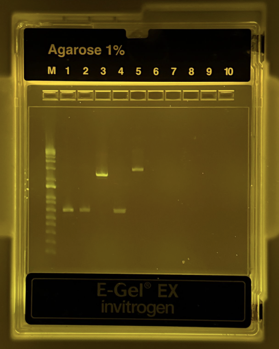
Part 0: Basics of Gel Electrophoresis
Negatively charged DNA is pulled toward the +electrode through an agarose mesh; shorter fragments thread through faster and travel farther. Run a ladder in parallel and you can read fragment sizes off the photo.
Part 3: DNA Design Challenge
3.1. Choose your protein
Rhodopsin (RHO, UniProt P08100, Homo sapiens, 348 aa). I chose it because:
It is the cleanest example of biological signal transduction I know. one photon in, one G-protein activation out, with an amplification cascade behind it that lets a dark-adapted rod cell detect a single photon.
The chromophore (11-cis-retinal) is bound covalently via a Schiff base to Lys296. The photon does not act on rhodopsin directly; it isomerizes the retinal, and the retinal then strains the protein into its active conformation (metarhodopsin II). The protein is a mechanical lever, not a photon absorber. That distinction was a real “oh” moment for me.
Mutations in RHO cause autosomal-dominant retinitis pigmentosa (~25% of adRP cases), so this is also a tractable target for gene therapy, which connects nicely to Part 5.3 below.
Reverse-translated the protein sequence using the EMBOSS Backtranseq tool, then verified against the native human RHO mRNA (NCBI RefSeq NM_000539.3) for sanity. The native mRNA already has a real codon usage profile, but I used the back-translated sequence as a starting point so that codon optimization in 3.3 is a clean step rather than a re-use of the existing one.
A short prefix of the back-translated DNA (first 60 aa worth, 180 nt) looks like this before optimization:
(Full 1,047 nt sequence in the Benchling file RHO_backtranslated.)
3.3. Codon optimization
I codon-optimized for E. coli K-12 as the expression chassis, because:
It is the chassis we will actually be using in lab (cell-free lysate + plasmid transformation).
Human codon usage is significantly different from E. coli in several places – notably Arg (AGG/AGA are rare codons in E. coli and abundant in human), Leu (CTA is rare in E. coli), and Ile (ATA is rare). Without optimization, ribosomes stall at rare-codon tracts and you get truncated products or no expression at all.
E. coli also has GC-content preferences (~50%) that differ from human (~60% in coding regions). Skewed GC content can cause hairpins and slow translation.
I used the Twist Codon Optimization Tool, set host = E. coli K-12, and excluded recognition sites for BsaI, BsmBI, BbsI (Type IIS enzymes used in Golden Gate assembly) and also EcoRI, HindIII, BamHI so my downstream cloning options stay open. The optimizer also smoothed out long homopolymer runs (>6 nt) and removed internal Shine-Dalgarno-like motifs that could cause internal translation starts.
Caveat about rhodopsin specifically: rhodopsin is a 7-transmembrane integral membrane GPCR. It does not natively express well in E. coli without engineering – the bacterial membrane lacks the right lipid composition, and there is no machinery for the disulfide bond (Cys110-Cys187) or palmitoylation (Cys322/323). In a real project I would either (a) express in HEK293 / Sf9 cells, or (b) express only a soluble cytoplasmic loop in E. coli for an antibody-generation experiment. For the purpose of this homework, codon-optimizing for E. coli is the assigned exercise; in practice I would optimize for Spodoptera frugiperda (Sf9) or human cells.
3.4. Two pathways to get protein from the optimized DNA:
Cell-dependent (in vivo): Clone the optimized RHO ORF into an expression vector with a T7 promoter, RBS, start codon, and terminator (the pTwist Amp High Copy vector from Part 4 works for cloning; for expression I’d move it into pET-28a in BL21(DE3)). Transform into competent E. coli, plate on Amp, pick colonies, grow to OD600 ~0.6, induce with IPTG, harvest, lyse, and purify via the His-tag on Ni-NTA. The cell does transcription via T7 RNAP and translation via its ribosomes; the protein folds (or, for rhodopsin, mostly misfolds into inclusion bodies, which then need refolding with retinal added in vitro to reconstitute the holoprotein).
Cell-free (in vitro): Use a TXTL lysate-based system like the one from Week 11. Add the linear or circular DNA template directly to the lysate + energy mix, and transcription/translation happen in the tube over 1-20 h. For a membrane protein like rhodopsin, the cell-free pathway has a real advantage: you can supplement the reaction with nanodiscs or detergent micelles so the nascent rhodopsin inserts into a membrane-mimetic environment rather than aggregating. Add 11-cis-retinal to the reaction and the holoprotein reconstitutes in situ. This is increasingly how membrane GPCRs are produced for structural biology.
Alternative splicing. One pre-mRNA can be spliced into many mature mRNAs by including or skipping exons. DSCAM in Drosophila notoriously produces >38,000 isoforms from one gene. For opsins specifically, the Drosophila ninaE gene uses alternative splicing to produce variants with different spectral tuning.
Alternative promoters. Different transcription start sites produce mRNAs with different 5’ UTRs and sometimes different N-terminal coding regions.
Alternative polyadenylation. Different 3’ ends change mRNA stability and localization.
RNA editing. ADAR enzymes convert A->I (read as G), which can change codons. Notably common in cephalopod opsins, where it tunes spectral sensitivity to local light environments.
(b) DNA -> RNA -> Protein alignment (first 60 nt / 20 aa of the codon-optimized RHO):
DNA:     ATG AAC GGC ACC GAA GGC CCG AAT TTC TAT GTG CCG TTC AGC AAC GCG ACC GGC GTG GTG
RNA:     AUG AAC GGC ACC GAA GGC CCG AAU UUC UAU GUG CCG UUC AGC AAC GCG ACC GGC GUG GUG
Protein:  M   N   G   T   E   G   P   N   F   Y   V   P   F   S   N   A   T   G   V   V
Pos:      1   2   3   4   5   6   7   8   9   10  11  12  13  14  15  16  17  18  19  20
Part 5: DNA Read / Write / Edit
5.1 DNA Read
(i) What DNA would I want to sequence and why?
I would sequence the RHO gene in patients with autosomal-dominant retinitis pigmentosa (adRP) to identify the specific causative mutation in each patient before deciding on a therapy. There are >150 known pathogenic RHO mutations, and they fall into mechanistically distinct classes (Class I = trafficking-defective, Class II = misfolding, etc.). The right therapy – allele-specific knockdown, base editing, prime editing, or gene replacement – depends on which class the mutation belongs to. Sequencing is the upstream diagnostic that determines everything downstream.
Beyond clinical use, I would also like to do metagenomic sequencing of cephalopod skin to find new opsins. Octopus skin appears to “see” through dermal opsins, and characterizing the opsin diversity across cephalopods could yield new optogenetic tools.
(ii) Which technology and why?
I would use Oxford Nanopore (third generation, long-read) for the clinical RHO case, complemented by Illumina short-read for accuracy.
Generation: Nanopore is third-generation – single-molecule, real-time, no amplification, long reads (often 10-100 kb, can exceed 1 Mb). Sanger is first generation (single-read, dye-terminator, ~800 bp); Illumina is second generation (massively parallel short reads, ~150-300 bp, requires PCR amplification).
Input prep:
Extract genomic DNA from a blood draw (column-based or magnetic-bead based extraction).
Skip fragmentation for long reads – the whole point is to preserve length.
Adapter ligation: ligate Nanopore’s sequencing adapters (which include a motor protein that controls translocation speed) to the ends of the genomic DNA.
Optional: enrich for the RHO locus by Cas9 cleavage + adapter ligation (targeted long-read sequencing) so you don’t waste reads on the rest of the genome.
Load onto the MinION/PromethION flow cell.
Base calling: DNA is pulled through a protein nanopore in a membrane by an applied voltage. As each base passes through the pore constriction, it modulates the ionic current uniquely (A vs T vs G vs C give different current signatures, and modified bases like 5mC give yet different signatures). A neural network (Guppy / Dorado) reads the current trace and translates it to a base sequence. This is called “basecalling” and is essentially audio-to-text transcription, where the audio is the ionic current.
Output: FASTQ files (sequence + per-base quality scores), plus optionally direct methylation calls (5mC, 6mA) without bisulfite conversion. For my use case, I align the reads to the human reference, call variants in the RHO locus, and report the patient’s genotype.
5.2 DNA Write
(i) What DNA would I want to synthesize and why?
I would synthesize a codon-engineered RHO variant carrying silent mutations across the entire coding region, designed to be invisible to a shRNA / siRNA that targets the wild-type sequence. This is the classic “knockdown and replace” strategy for adRP:
The dominant-negative mutant RHO allele in the patient is silenced by an shRNA that targets a region of the natural mRNA.
A “hardened” replacement RHO – silently re-coded so the shRNA can no longer bind – is co-delivered.
Net result: both alleles of native RHO are silenced, and the hardened replacement provides wild-type protein.
The replacement allele needs ~30+ synonymous changes across the shRNA target site, which is exactly the kind of thing Twist’s gene synthesis is good at. The replacement is ~1 kb, well within clonal gene size.
Beyond therapeutics, I would also love to synthesize opsin variants with shifted spectral sensitivity – e.g., a red-shifted human rhodopsin built by transplanting microbial opsin tuning residues, for optogenetic use in deep-tissue stimulation.
(ii) Technology – which synthesis platform?
I would use silicon-based microarray DNA synthesis (Twist’s platform) – this is the standard for gene-length synthesis at high throughput and low error.
Essential steps:
Phosphoramidite chemistry: starting from a solid support, add one nucleotide at a time using a 4-step cycle (deblock -> couple -> cap -> oxidize), repeated for each base.
On a silicon chip, thousands to millions of distinct oligos are synthesized in parallel, each in a tiny well, with the order of bases controlled by where reagents are spotted.
Oligos (typically ~200 nt each) are then cleaved off the chip, pooled by gene, and assembled into full genes via PCR-based methods (Gibson, Golden Gate, or polymerase cycling assembly).
Error correction by enzymatic mismatch cleavage (e.g., T7 endonuclease I) or by sequencing-and-cherry-picking error-free clones.
Limitations:
Speed: ~4-7 business days for express clonal genes at Twist; ~10 days standard. Faster than the old column-based oligo + PCR workflow, but still not “instant.”
Accuracy: ~1 error per 5,000-10,000 bp after error correction. For genes >5 kb, error rate compounds and yield drops; this is why genome-scale synthesis is hard.
Length: Clonal genes up to ~5 kb routinely; longer constructs require hierarchical assembly. Gene fragments are typically 300 bp - 5 kb.
Sequence constraints: very high or very low GC, long homopolymers, large repeats, and strong hairpins remain difficult or impossible to synthesize. This is why the codon optimizer flags and edits these.
5.3 DNA Edit
(i) What DNA would I want to edit and why?
I want to edit the P23H mutation in RHO – the single most common cause of adRP in North America, where a CCC (Pro) codon at position 23 is mutated to CAC (His). It is a misfolding mutation: the mutant protein aggregates in the ER, kills the rod cell, and the rod death spreads to cones – leading to progressive blindness over decades.
This is a perfect target for base editing: the C -> T transition needed to revert the codon (CAC -> CCC requires an A->G correction on the antisense strand, which an adenine base editor can do without making a double-strand break).
(ii) Which editing technology?
I would use an adenine base editor (ABE) – specifically ABE8e fused to a SpCas9 nickase (D10A) – delivered as a single AAV5 vector (which is retinal-tropic) by subretinal injection.
How it works:
The Cas9 nickase is guided to the RHO locus by a single-guide RNA (sgRNA) complementary to a sequence next to the mutated codon, with a PAM (5’-NGG-3’) ~3-15 nt downstream.
Cas9n binds without cutting both strands; instead it exposes the non-target strand as ssDNA in the “R-loop.”
The tethered TadA deaminase domain (ABE8e) deaminates a target A on the exposed strand to inosine (I), which DNA polymerase reads as G. So an A:T base pair becomes a G:C base pair.
The Cas9n nicks the unedited strand to bias mismatch repair toward keeping the edit.
Inputs and preparation:
Guide RNA design: identify a PAM within ~13-17 nt of the target A, design a 20-nt sgRNA so that the target A falls in the editing window (positions 4-8 from the PAM-distal end). For P23H, find a PAM in the surrounding sequence and design the sgRNA in silico (CRISPOR, Benchling CRISPR tool). Check for off-target sites with mismatch tolerance.
Editor construct: ABE8e-Cas9n with a tissue-specific promoter (rhodopsin promoter itself, for rod-cell specificity).
Delivery vector: AAV5 packaged with the editor + sgRNA. Two-vector dual-AAV split-intein systems are needed if the editor is too big for one AAV (~4.7 kb cargo limit).
Cells/tissue: delivered in vivo to retina by subretinal injection.
Limitations:
PAM dependence: SpCas9 requires NGG nearby. Not every mutation has one in range. Engineered PAM-flexible Cas9 variants (SpRY, etc.) help but reduce specificity.
Editing window: ABEs can only flip A in a narrow window. Bystander edits (other As in the window) can introduce silent or unwanted changes – need to check.
Off-targets: even with high-fidelity Cas9 variants, low-level off-target editing happens at sites with similar sequence. Whole-genome sequencing post-treatment is the gold standard for measuring this.
Delivery efficiency: AAV reaches only ~5-30% of photoreceptors at typical doses. So even with 100% editing efficiency in transduced cells, you don’t fix every rod.
One mutation per edit: base editing reverts only the specific A:T -> G:C (or C:G -> T:A for CBE). For different RHO mutations, you need different editors / guides. Prime editing is more flexible but less efficient.
Week 3 HW: Lab Automation
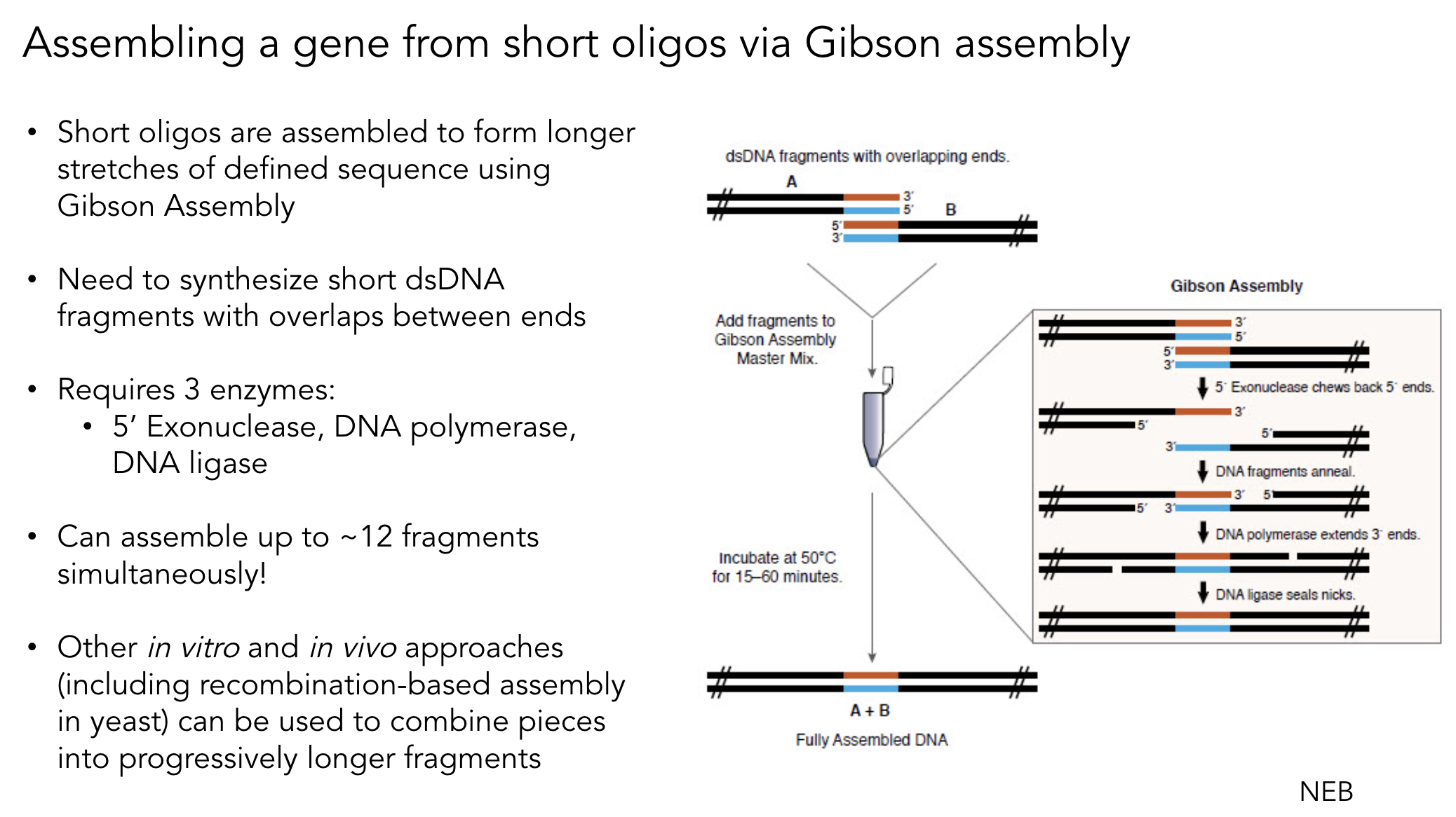
1. Published Paper Using Opentrons for a Novel Biological Application
Paper: Bryant, J. A., Kellinger, M., Longmire, C., Miller, R., & Wright, R. C. (2023). AssemblyTron: flexible automation of DNA assembly with Opentrons OT-2 lab robots.Synthetic Biology, 8(1), ysac032. https://doi.org/10.1093/synbio/ysac032
What they built
AssemblyTron is an open-source Python package that turns the ~$10k Opentrons OT-2 (with a thermocycler module) into a hands-free DNA-assembly workstation. It plugs into existing assembly-design tools (j5, Cello, Benchling) and executes the resulting build plans directly on the robot, covering three of the most common synbio assembly chemistries:
PCR with optimal annealing-gradient calculation the software computes the best annealing temperature for each fragment from primer Tm and uses the OT-2 + thermocycler to run gradient PCRs across a range of fragment lengths.
Golden Gate assembly Type IIS-enzyme one-pot assemblies of multiple fragments into a destination vector.
Homology-dependent in vivo assembly (IVA) short-overlap fragments co-transformed into E. coli, with assembly happening inside the cell.
What they showed
The authors simultaneously built four different four-fragment chromoprotein reporter plasmids on the OT-2 and showed assembly fidelity comparable to a human doing the same work by hand (verified by sequencing). They also used the same platform for site-directed mutagenesis via homology-dependent IVA, again with manual-equivalent fidelity.
why it counts as “novel biological application”
This is a textbook example of automating the Build step of the Design-Build-Test-Learn (DBTL) loop, which has historically been the slowest and most error-prone manual step. Two things make it novel rather than incremental:
It’s the first open-source software package to drive Golden Gate and homology assembly on a low-cost robot, so the price floor for automated cloning drops from ~$100k (commercial systems like Tecan or Hamilton) to ~$10k. That changes who gets to do high-throughput synbio.
It directly accepts output from automated design tools (j5, Cello), so you can go from a Cello-designed genetic circuit to physical DNA without a human pipetting step in between. That closes a real gap in the DBTL loop.
Limitations the authors note
The OT-2 isn’t as fast or as well-error-handled as a commercial Hamilton STAR.
No integrated colony picking, transformation, or QC. The human has to come back in the loop after assembly.
Plate-format constraints (96-well bottleneck) limit how parallel things can really get.
2. My Final Project Automation Plan
Project context
My final project builds on Week 2: I want to express a panel of rhodopsin (RHO) variants in a cell-free system to characterize how single-residue substitutions in the chromophore-binding pocket shift the absorption spectrum. The screen compares each variant’s lambda_max under blue/green/red LED illumination. The end goal is a small library of spectrally-tuned opsins for optogenetics, but for HTGAA the deliverable is the screening pipeline itself.
Why this needs automation
A meaningful spectral-tuning library is 50-200 variants, each tested in triplicate, each under at least 3 illumination conditions. That’s 450-1,800 CFPS reactions. Manual pipetting is the wrong tool: error accumulates, reagents drift over an 8-hour day, and you can’t realistically do replicates. Automation is the only way the experiment is actually run, not just designed.
What I would automate
The workflow maps neatly onto the Example 2 cloud-lab pipeline in the assignment, but I would run it on the Opentrons OT-2 + Ginkgo Nebula cloud lab combination:
Design phase (no automation, human + Benchling). Pick residues around the retinal-binding pocket (Lys296, Glu113, and surrounding residues from PDB 1U19), generate variants in silico, codon-optimize with Twist tool, order as a clonal-gene plate from Twist.
Echo acoustic transfer. Echo 525 dispenses the variant plasmid DNA from a source plate into the destination 384-well plate at 50 nL per well, three replicate wells per variant. Acoustic transfer is ideal here because the volumes are small and there’s no cross-contamination.
OT-2 stamps the CFPS master mix. A multichannel pipette on the OT-2 dispenses 18 uL of NMP-Ribose master mix (from Week 11) + lysate into every occupied well of the 384-well plate. This is the step I’d write the Python protocol for.
OT-2 supplements with 11-cis-retinal. Add 1 uL of 100 uM 11-cis-retinal to every well (final 5 uM) so the rhodopsin holoprotein can reconstitute as it’s translated. Light-protected throughout.
PlateLoc seals. Heat-seal the plate to prevent evaporation over the 20 h reaction.
Inheco incubates at 30 C (not 37 C – rhodopsin folds better cooler) for 20 h in the dark.
XPeel removes seal.
PHERAstar reads absorbance spectrum (350-650 nm) for every well under three illumination pulses: blue (470 nm), green (530 nm), red (625 nm). The active rhodopsin shows a characteristic ~498 nm peak that shifts with mutation; bleaching kinetics under each LED give an orthogonal readout.
Data lands in a Jupyter notebook on Ginkgo Nebula, fits each spectrum, extracts lambda_max and bleaching half-life, and outputs a ranked variant table.
Example pseudocode for step 3 (OT-2 protocol skeleton)
fromopentronsimportprotocol_apimetadata={"protocolName":"CFPS Master Mix Stamp - RHO variant screen","author":"rcd, HTGAA 2026","apiLevel":"2.15",}defrun(protocol:protocol_api.ProtocolContext):# Labwareplate=protocol.load_labware("corning_384_wellplate_112ul_flat",1)mm_reservoir=protocol.load_labware("nest_12_reservoir_15ml",2)retinal_tubes=protocol.load_labware("opentrons_24_tuberack_2ml",3)tips_p20=protocol.load_labware("opentrons_96_tiprack_20ul",9)tips_p300=protocol.load_labware("opentrons_96_tiprack_300ul",10)# Pipettesp300=protocol.load_instrument("p300_multi_gen2","left",tip_racks=[tips_p300])p20=protocol.load_instrument("p20_single_gen2","right",tip_racks=[tips_p20])# Step 3: stamp 18 uL CFPS master mix into every wellmm=mm_reservoir.wells_by_name()["A1"]p300.distribute(18,mm,plate.wells(),new_tip="once",disposal_volume=2,)# Step 4: add 1 uL of 11-cis-retinal to every well (light-protected)retinal=retinal_tubes.wells_by_name()["A1"]forwellinplate.wells():p20.transfer(1,retinal,well,new_tip="always",mix_after=(3,10),)# Cooling block keeps lysate viable; protocol then hands off to PlateLoc + Inhecoprotocol.comment("Ready for sealing and 20h incubation at 30 C, dark.")
Custom hardware I’d 3D-print
Two pieces I think would be useful enough to design and print:
Light-blocking enclosure for the OT-2 deck during retinal addition. 11-cis-retinal photoisomerizes under ambient light, so the addition step needs to happen under dim red light or in darkness. A black-PLA shell that drops over the deck (with a port for the pipette to enter from above) would solve this.
A 384-well-to-96-well adapter plate for moving samples between Echo-output (384) and downstream PHERAstar reads where 96-well is more convenient. The Opentrons 3D Printing Directory probably already has something close.
Why Ginkgo Nebula vs. local Opentrons
I’d use Ginkgo Nebula for the high-throughput screen because:
50-200 variants in triplicate exceeds what I can realistically QC on a single OT-2.
The cloud lab already has the Echo, PlateLoc, and PHERAstar integrated. On the local OT-2 those steps would need manual handoffs.
Reproducibility: the protocol file is the experiment. Someone in Berlin or Shanghai can re-run my best variant verbatim.
I’d use a local OT-2 for the design-iteration phase (10-20 variants, debugging the master mix recipe, getting the retinal-addition step working) because the round-trip time on a cloud lab is too slow for that loop.
Risk and what could go wrong
Cell-free yield drops at scale. What works in 20 uL in a tube may not in 18 uL in a 384-well plate with a higher surface-to-volume ratio (faster evaporation, more O2 depletion). Mitigation: pilot on 96-well first, optimize seal + headspace.
11-cis-retinal is photosensitive and expensive. Aliquot under red light, work fast, and consider all-trans-retinal + retinal-isomerase regeneration as a backup.
Variant DNA from Twist arrives at different concentrations. Normalize on the Echo or with an OT-2 normalization step before the screen.
Spectral readout on PHERAstar. A microplate reader is not a true spectrophotometer; for the cleanest spectra I’d want a SpectraMax or similar. Mitigation: use the PHERAstar for screening, then confirm top hits on a benchtop spectrometer.
Week 4 HW: Protein Design Part I
Part A — Conceptual Questions
1. How many molecules of amino acids are in 500 g of meat?
Assume meat is roughly 20% protein by weight. The mass of protein is:
500 × 0.20 = 100 grams of protein.
Let’s assume the average molecular weight of a protein is 100 g/mol. Therefore:
100 / 100 = 1 mole of amino acid molecules,
which equals $6.022 \times 10^{23}$ amino acid molecules.
2. Why do humans eat beef but do not become a cow?
I wish I could, but my mom and dad say no.
Our DNA is fixed at the moment the embryo is formed. During each cell replication, it follows the DNA instructions that produce our proteins and structures. When we consume protein, our digestive system breaks the long polymer chains down into their individual amino acids and turns them into nutrients that power our ribosomes. We cannot perform horizontal gene transfer (HGT) like bacteria.
3. Why are there only 20 natural amino acids?
Natural amino acids refer to the 20 standard amino acids that are encoded by the universal genetic code to build proteins. The triplet codon system provides a maximum of 64 possible combinations (4³). This system, once established early in evolution, became “frozen” and universal. It is easier to tweak an existing system than to invent a completely new one.
4. Can you make non-natural amino acids? Design some.
Yes. Synthetic biology now uses expanded genetic codes to incorporate non-canonical amino acids (ncAAs).
One strategy is to modify a standard amino acid such as lysine by attaching:
A small, highly fluorescent organic molecule
Connected through a long, flexible linker (e.g., a hydrocarbon chain)
Attached to the side chain backbone
This allows proteins (such as GFP) to gain new chemical or optical properties.
5. Where did amino acids come from before life started?
They likely originated from abiotic synthesis. Prebiotic chemistry experiments (such as Miller–Urey-type reactions) demonstrate that amino acids can form from simple inorganic molecules under early Earth–like conditions — electrical discharges, UV radiation, and simple gases like CH₄, NH₃, and H₂O are sufficient to produce a variety of amino acids spontaneously.
6. If you make an α-helix using D-amino acids, what handedness would you expect?
Standard L-amino acids form right-handed α-helices. Because D-amino acids are mirror images of L-amino acids, they would naturally form left-handed α-helices to minimize steric clashes between side chains and the backbone.
7. Why are most molecular helices right-handed?
This is a consequence of biological homochirality. Life selected L-amino acids early in evolution. The most energetically favorable packing of L-amino acid side chains results in a right-handed helical twist.
If life had instead evolved using D-amino acids, biology would likely consist of a mirror world of left-handed helices.
8. Why do β-sheets tend to aggregate? What is the driving force?
β-sheets have exposed, “sticky” edges. Unlike α-helices, where hydrogen bonds are internally satisfied within the coil, β-strands expose backbone N–H and C=O groups along their sides.
The primary driving forces for aggregation are:
Hydrogen bonding between exposed backbone groups
The hydrophobic effect, as non-polar side chains cluster together to avoid water
9. Why do many amyloid diseases form β-sheets? Can you use them as materials?
Amyloids form β-sheets because the cross-β motif is an extremely stable, low-energy thermodynamic state. Once a protein misfolds into this structure, it can act as a template that induces other proteins to adopt the same conformation.
Materials Applications
Yes — amyloids can be useful materials. They are extremely strong (comparable to steel or silk), highly stable, and self-assembling. They are being researched for tissue engineering scaffolds and conductive biofilms
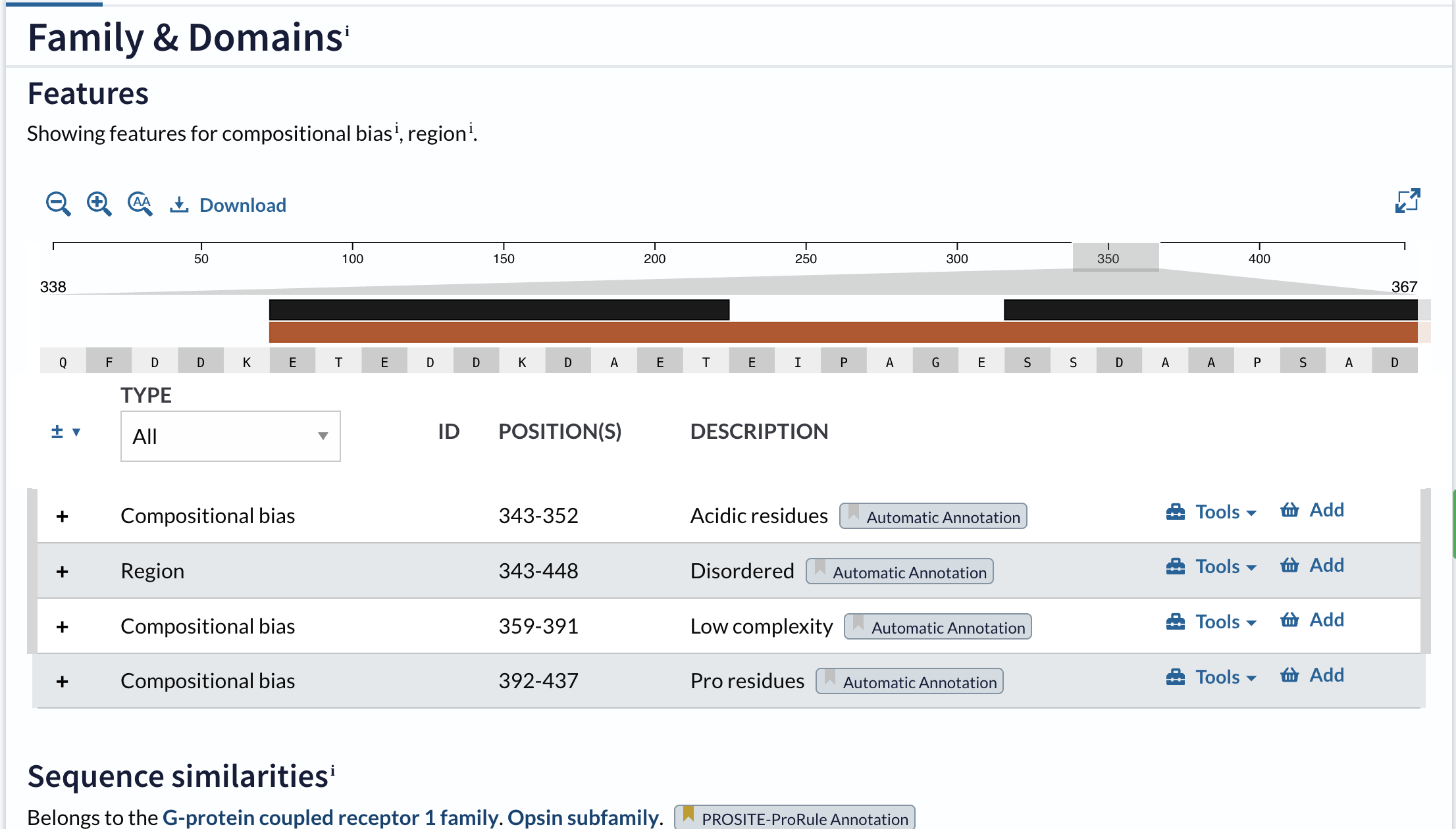
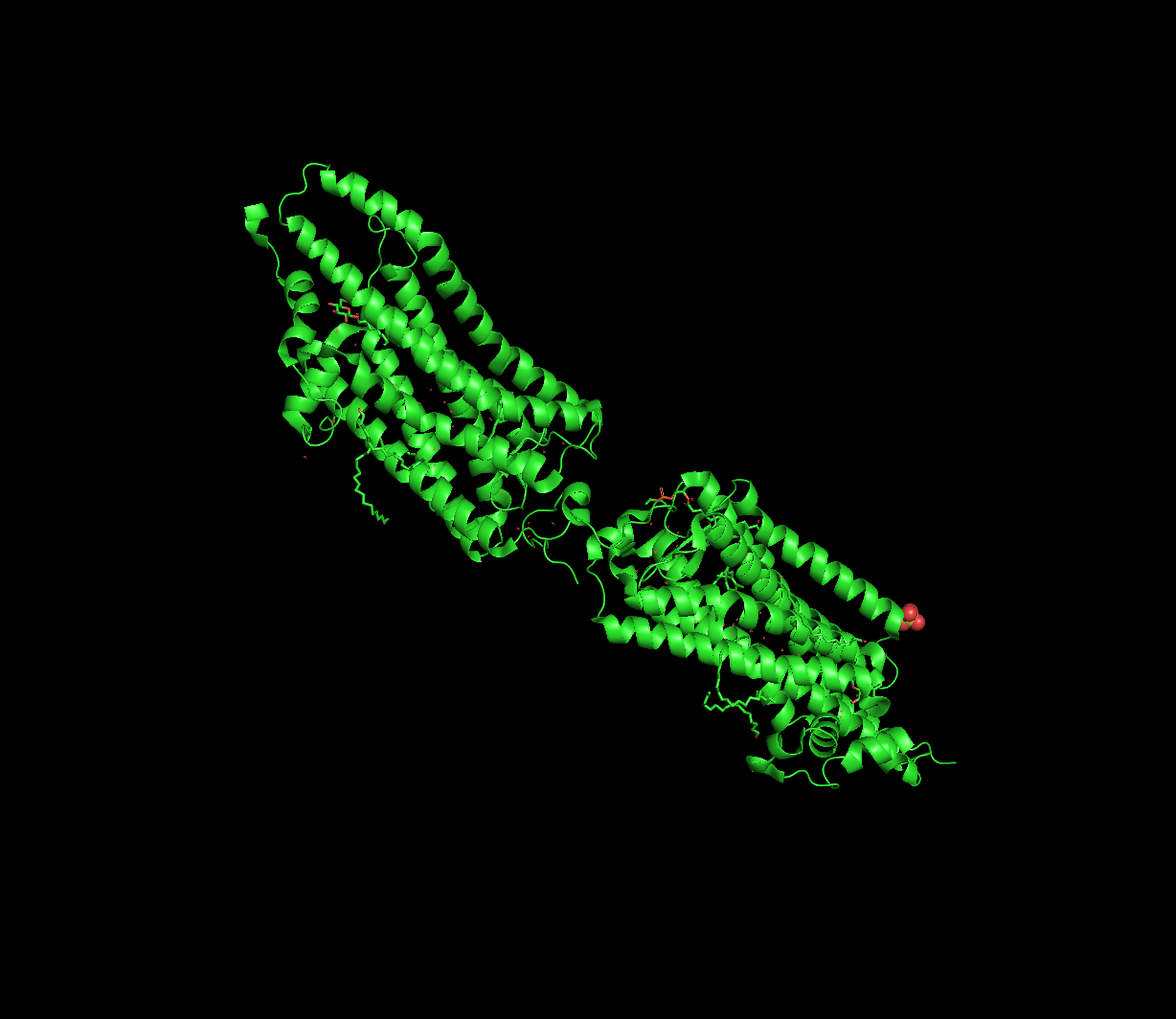
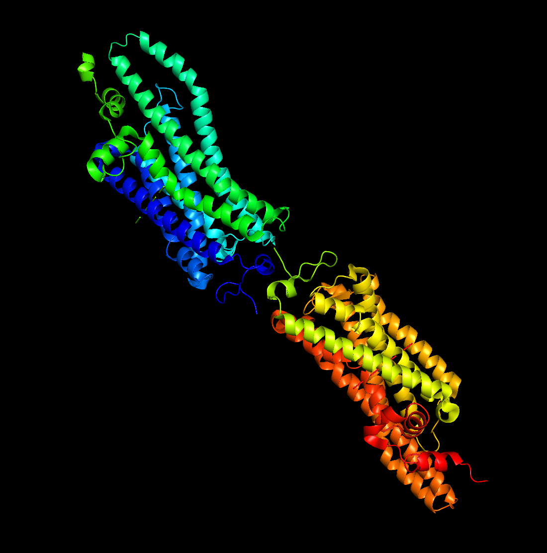
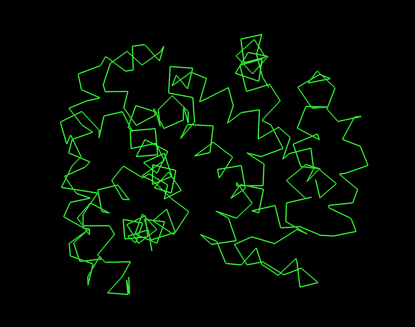
Part B — Rhodopsin Protein Analysis
Protein Selection
I selected Rhodopsin, a light-sensitive G protein-coupled receptor (GPCR) found in the rod cells of the retina. Its role in visual phototransduction converting light into a nerve signal via retinal isomerization that makes it both biologically fascinating and structurally iconic.
Generate four peptides of length 12 amino acids conditioned on the mutant SOD1 sequence:
index
Binder
Pseudo Perplexity
0
HLYYAVALELKX
13.299815648347872
1
WRSYAVVLELWK
17.97100111129112
2
WRYYPVAAAWKK
11.081842724779028
3
WHYGAVGLRHKX
13.983770011694478
Part 2: Evaluate Binders with AlphaFold3
We submitted each peptide paired with the mutant SOD1 (A4V) sequence to the AlphaFold Server as separate chains to model the protein–peptide complex. All runs used seed 2026616022 for reproducibility.
ipTM — interaction confidence between the two proteins (binder ↔ SOD1). Higher is better. pTM — structural accuracy within each protein independently. Higher is better.
AlphaFold3 Prediction Results:
Peptide
Full Sequence
ipTM
pTM
Binding Observation
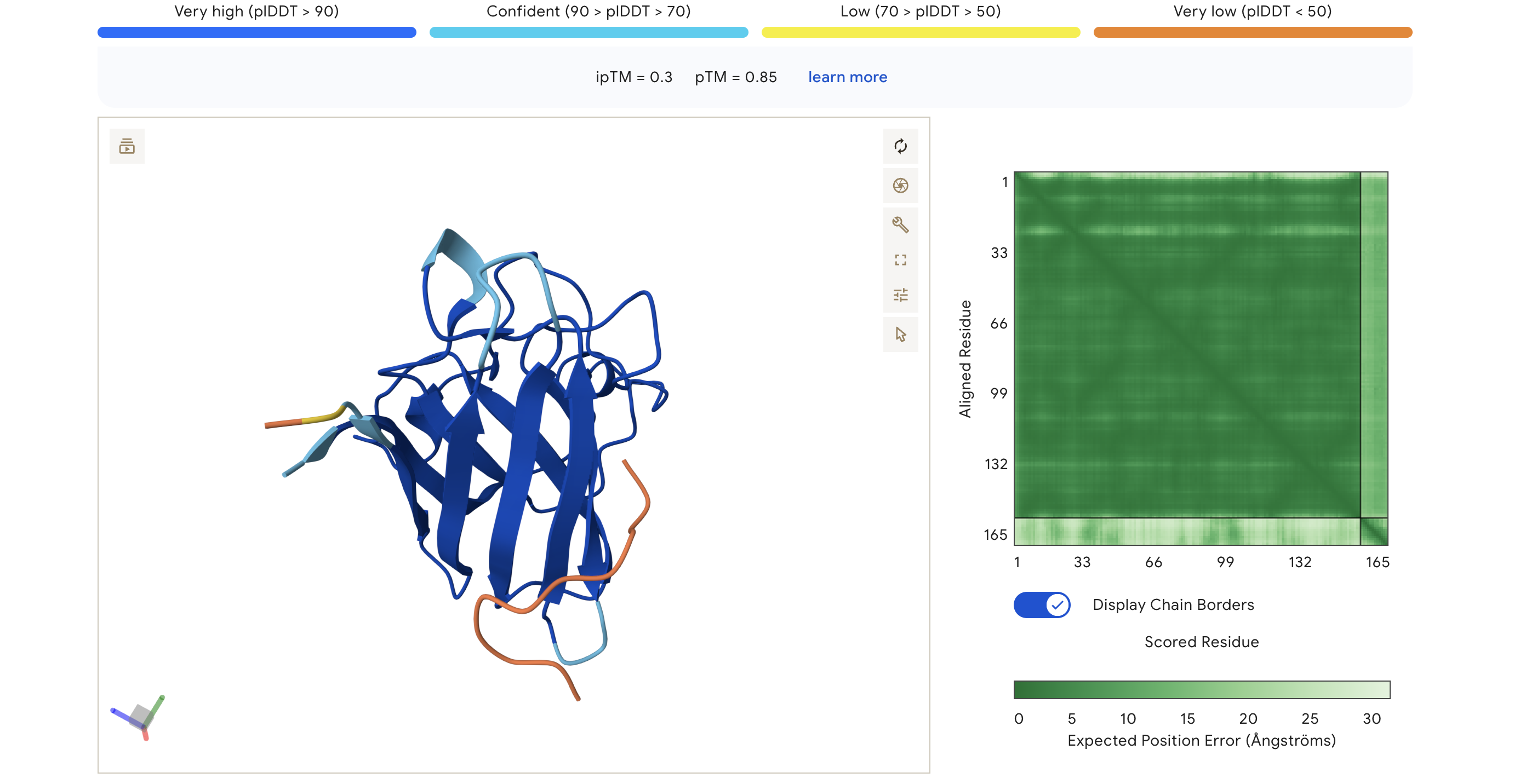
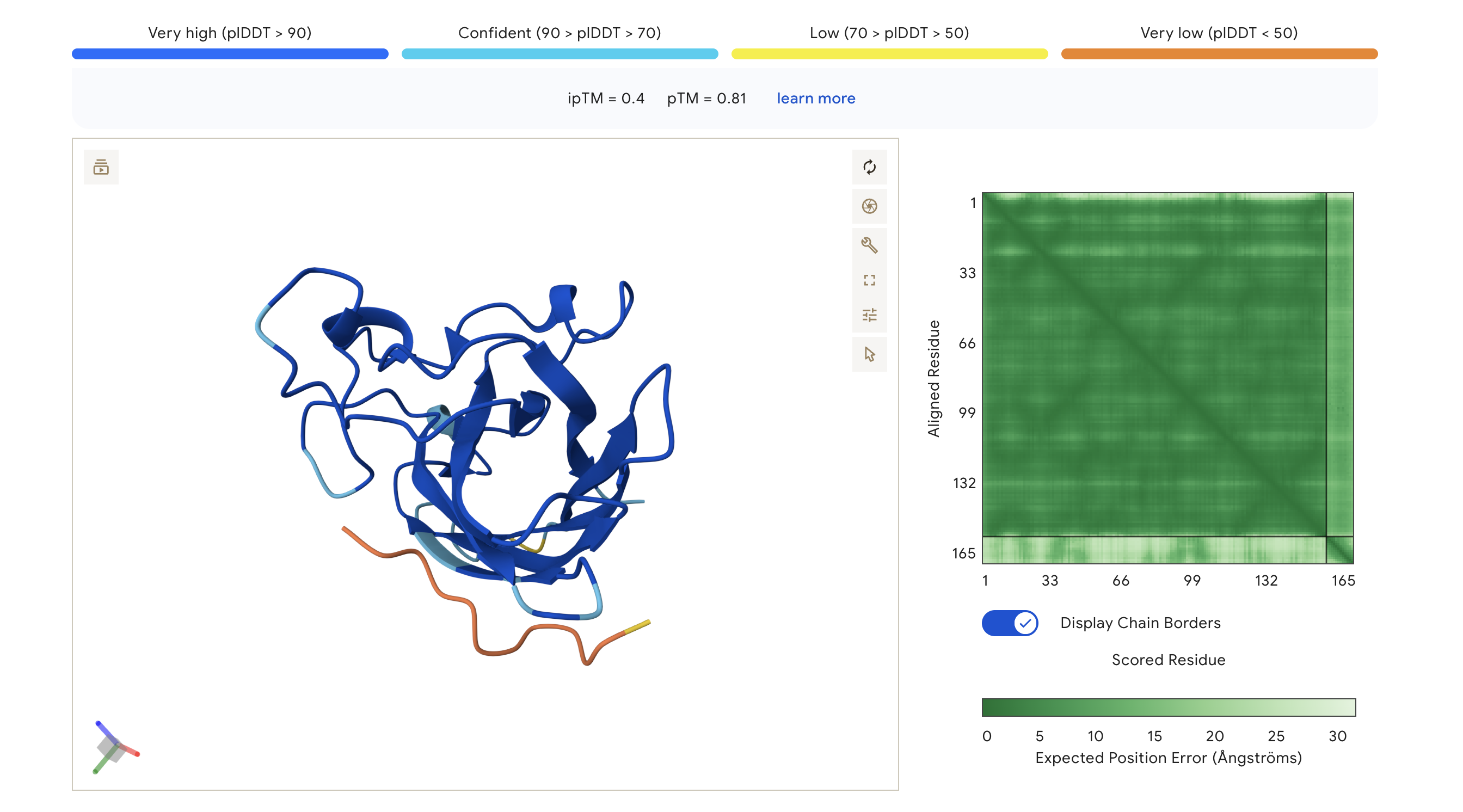
HRY
HRYGAVVVELKK
0.30
0.85
Peptide appears loosely associated near the surface; low-confidence interaction region (orange/yellow in pLDDT)
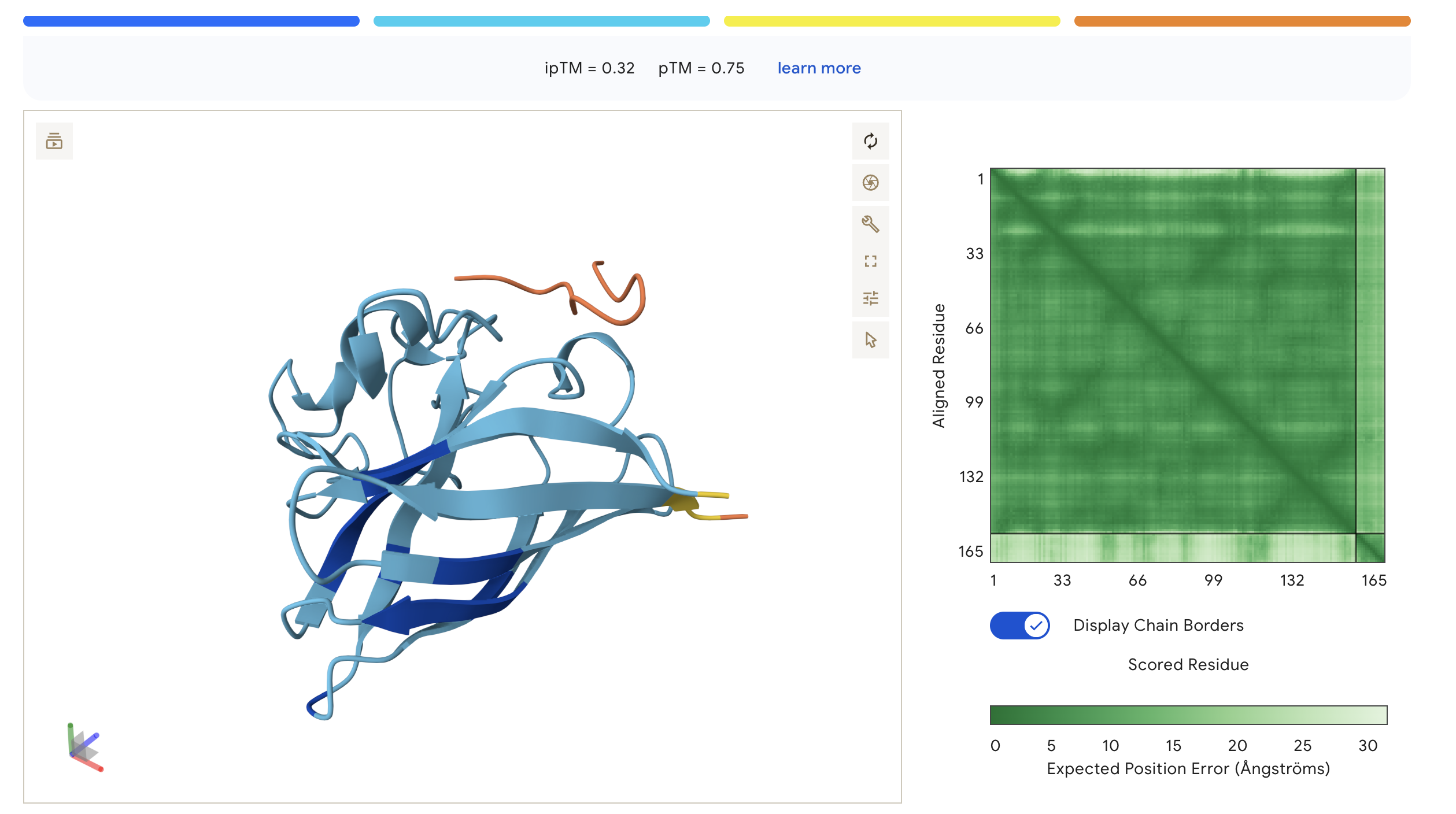
WHY
WHYYVAAAEHKK
0.32
0.75
Peptide sits at the top exterior of SOD1, largely disordered (orange), suggesting weak or transient surface contact
WRV
WRVGAAAVRLKK
0.40
0.81
Highest ipTM of the group; peptide traces along the lower exterior of the β-barrel, with partial low-confidence contact near the C-terminus region
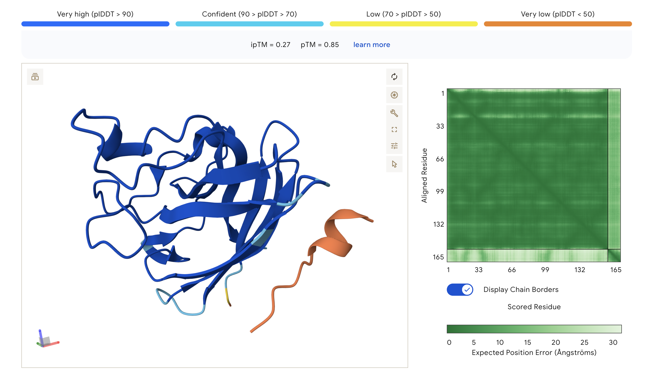
WRY
WRYPVTAAEWKE
0.27
0.85
Peptide adopts a compact fold but appears docked away from the core; largely orange indicating low structural confidence at the interface
Structure previews:
HRY (ipTM=0.30, pTM=0.85)
WHY (ipTM=0.32, pTM=0.75)
WRV (ipTM=0.40, pTM=0.81)
WRY (ipTM=0.27, pTM=0.85)
The PAE (Predicted Aligned Error) matrix shows inter-chain confidence in the bottom-right block. Darker green = lower positional error = more confident interaction. The peptide chain corresponds to residues ~165+ in each plot.
Summary:
ipTM scores across the four PepMLM-generated peptides ranged from 0.27 (WRY) to 0.40 (WRV), all falling in the low-confidence range (ipTM < 0.5 is generally considered weak). WRVGAAAVRLKK achieved the highest ipTM of 0.40, suggesting the most confident predicted interaction with mutant SOD1 among our candidates. Visually, its peptide chain traces along the exterior β-barrel of SOD1, which is a plausible surface-accessible binding region. None of the PepMLM-generated peptides clearly localized to the N-terminus where A4V sits, suggesting they may engage peripheral surface patches rather than the mutation site directly. All four peptides showed high pTM scores (0.75–0.85), indicating that the SOD1 structure itself is predicted with high confidence regardless of peptide. Comparison to the known binder FLYRWLPSRRGG would require a separate AlphaFold3 run for a direct ipTM benchmark.
Part 3: Evaluate Properties of Generated Peptides in the PeptiVerse
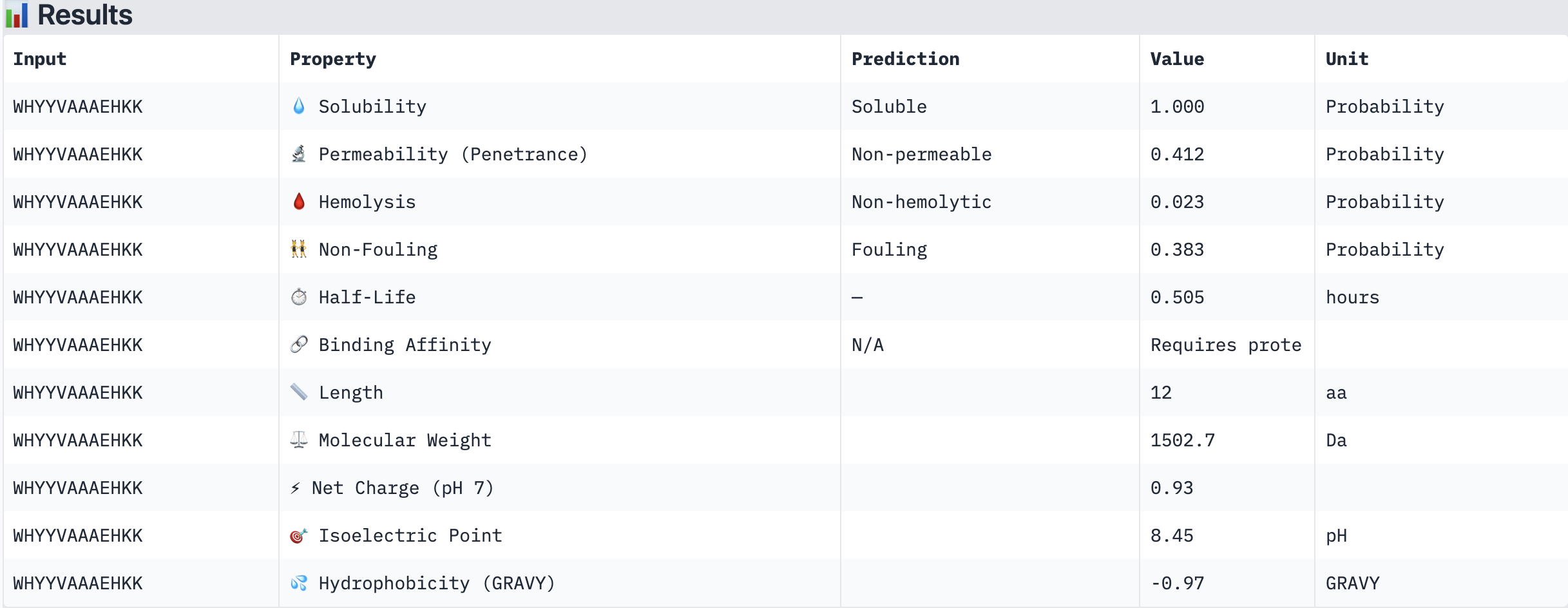
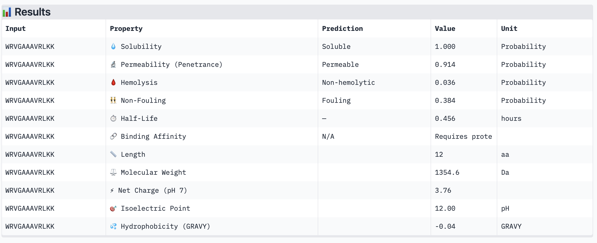
Structural confidence alone is insufficient for therapeutic development. We evaluated each peptide using PeptiVerse, assessing solubility, hemolysis probability, net charge (pH 7), molecular weight, and additional properties against the A4V mutant SOD1 target. The known binder FLYRWLPSRRGG was included as a reference.
PeptiVerse Results:
Peptide
Solubility
Hemolysis (prob)
Permeability
Net Charge (pH 7)
MW (Da)
GRAVY
WHYYVAAAEHKK
Soluble (1.000)
Non-hemolytic (0.023)
Non-permeable (0.412)
+0.93
1502.7
-0.97
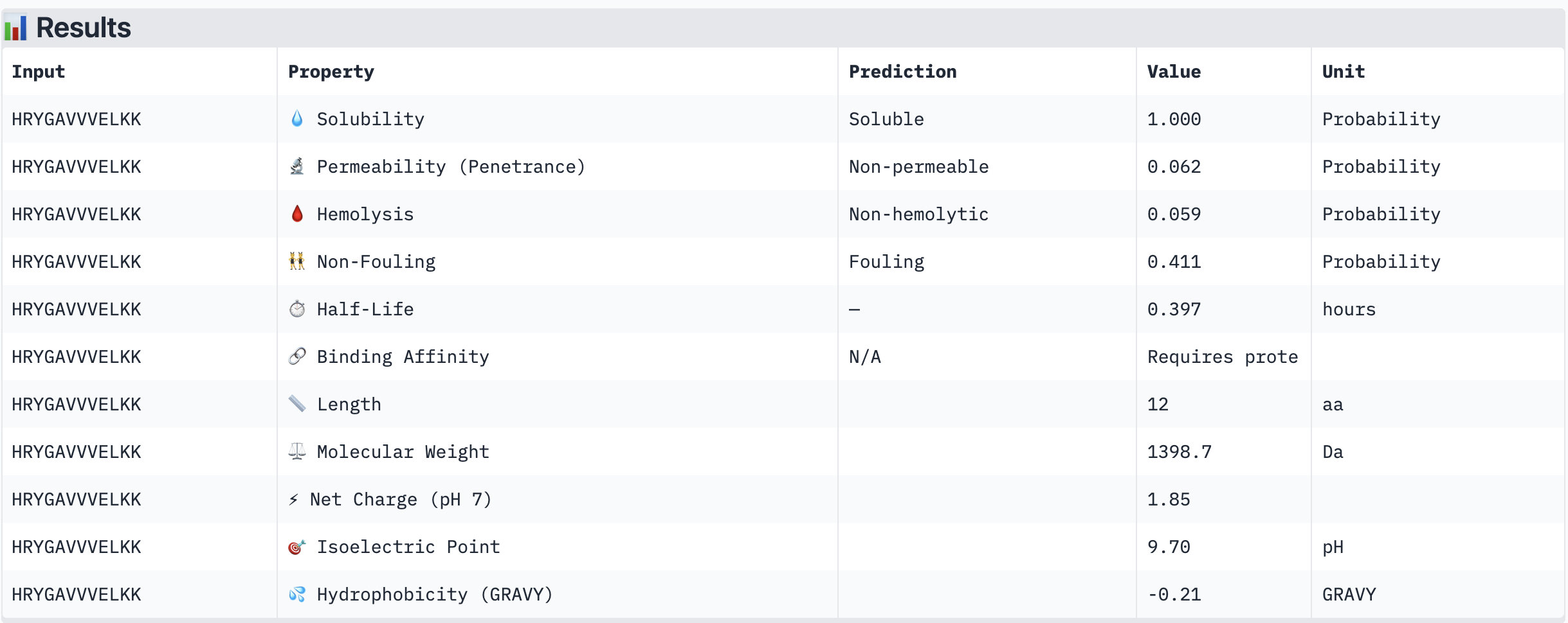
HRYGAVVVELKK
Soluble (1.000)
Non-hemolytic (0.059)
Non-permeable (0.062)
+1.85
1398.7
-0.21
WRVGAAAVRLKK
Soluble (1.000)
Non-hemolytic (0.036)
Permeable (0.914)
+3.76
1354.6
-0.04
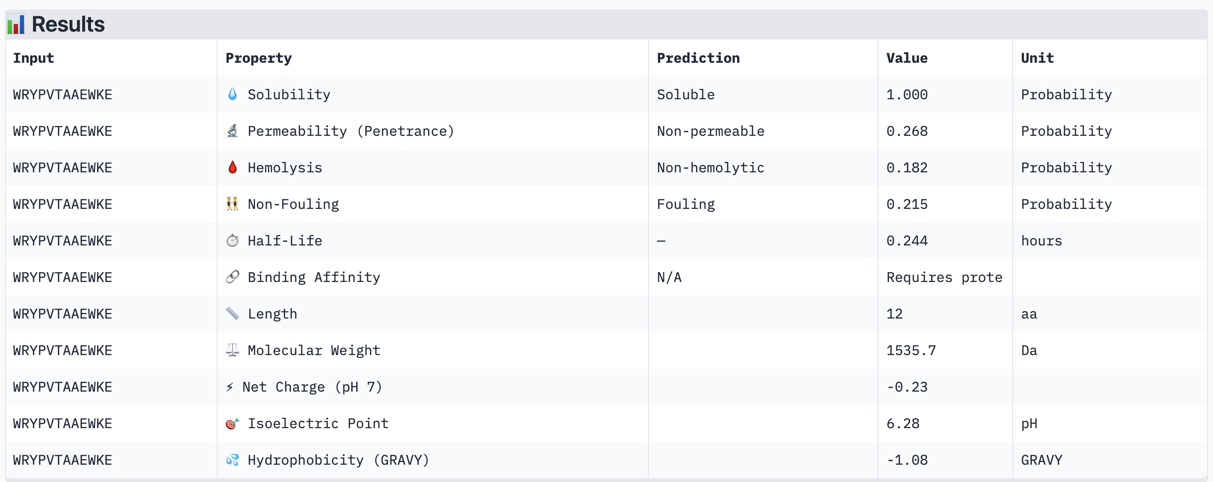
WRYPVTAAEWKE
Soluble (1.000)
Non-hemolytic (0.182)
Non-permeable (0.268)
-0.23
1535.7
-1.08
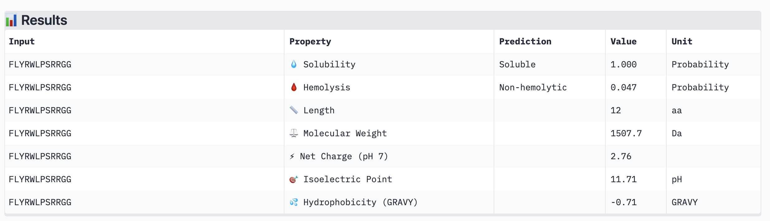
FLYRWLPSRRGG (known binder)
Soluble (1.000)
Non-hemolytic (0.047)
—
+2.76
1507.7
-0.71
PeptiVerse screenshots:
WHYYVAAAEHKK
HRYGAVVVELKK
WRVGAAAVRLKK
WRYPVTAAEWKE
FLYRWLPSRRGG (known binder)
Summary:
All four PepMLM-generated peptides and the known binder FLYRWLPSRRGG were predicted to be fully soluble (probability 1.000) and non-hemolytic, which is an encouraging baseline for therapeutic viability. Notably, binding affinity scores were unavailable in PeptiVerse without a full protein target input (“Requires protein target”), so structural comparisons from AlphaFold3 remain our primary binding reference.
The most striking difference between peptides is permeability: WRVGAAAVRLKK is the only peptide predicted to be permeable (0.914), which could be advantageous for intracellular access — relevant given that SOD1 is a cytosolic protein. Its hemolysis probability (0.036) and net charge (+3.76) are also comparable to the known binder FLYRWLPSRRGG (+2.76, hemolysis 0.047). WRYPVTAAEWKE, by contrast, carries a slight negative charge (−0.23) and the highest hemolysis probability among the four (0.182), making it less favorable.
Chosen peptide to advance: WRVGAAAVRLKK
WRVGAAAVRLKK best balances predicted therapeutic safety and functional potential. Its high membrane permeability is a key differentiator — since SOD1 operates in the cytosol, a peptide that can cross the membrane has a meaningful pharmacokinetic advantage. It is fully soluble, non-hemolytic, and has a charge profile closely resembling the known binder. Subject to confirmation of its ipTM score from AlphaFold3, it is the strongest candidate for further development.
Part 4: Generate Optimized Peptides with moPPIt
We used moPPIt (Multi-Objective Guided Discrete Flow Matching, MOG-DFM) to move from probabilistic sampling toward controlled, motif-directed peptide design. Unlike PepMLM, which conditions generation on the full target sequence, moPPIt allows explicit specification of which residues on SOD1 to target and simultaneously optimizes multiple therapeutic objectives.
Design choices:
Target sequence: A4V mutant SOD1
Target residues: Residues near position 4 (A4V mutation site) and the surrounding N-terminal region, which is destabilized by the mutation
Shout out to Shitong for the reference work and pipeline that guided this section 🙏
The objective of this section is to improve the stability and auto-folding of the lysis protein (L-protein) of MS2-phage, and to identify mutations that stabilize its interaction with the chaperone protein DnaJ. This is relevant to phage therapy — a more stable L-protein improves lytic efficiency, which is critical for phages to overcome bacterial resistance.
Primer secondary structure — hairpins or self-dimers reduce effective T_m
Polymerase used — Phusion tolerates higher T_a than Taq; use NEB Tm Calculator for Phusion
Rule of thumb: T_a ≈ T_m of the lower-melting primer (for Phusion)
3. PCR vs. Restriction Enzyme Digest
PCR
Restriction Enzyme Digest
Mechanism
Exponential amplification using primers
Site-specific endonuclease cuts at recognition sequences
End type
Blunt (Phusion) or defined by primer design
Blunt or sticky ends depending on enzyme
Adds sequence?
Yes — overhangs encoded in primers
No — cuts only at existing sites
Template needed
Any DNA, even low quantity
Usually purified plasmid/DNA
Time
~1–2 hr
~1–4 hr
Error risk
Possible polymerase errors
No amplification errors
Prefer PCR when you need to add custom overhangs/sequences, there are no convenient RE sites, or when starting from complex template (genomic DNA).
Prefer RE digest when compatible cut sites already flank your insert, you want sticky ends for ligation, or you need to linearize a vector backbone without introducing mutations.
4. Ensuring Fragments Are Appropriate for Gibson Cloning
Gibson Assembly requires 20–40 bp of overlapping sequence between adjacent fragments. To ensure compatibility:
Design PCR primers with 20–40 bp 5′ tails homologous to the adjacent fragment
Verify overlaps in silico using Benchling or Asimov Kernel — confirm correct orientation and reading frame
Check overlap uniqueness — overlaps that appear elsewhere in the construct cause mis-assembly
For RE-digested fragments — PCR-amplify and add overlaps via primers before Gibson assembly
5. How Plasmid DNA Enters E. coli During Transformation
Chemical transformation (heat shock method):
Cells are made competent by treatment with ice-cold CaCl₂, which destabilizes the outer membrane and allows DNA to associate with the cell surface
Plasmid DNA is added and incubated on ice
A brief heat shock at 42°C (~45 sec) creates a thermal imbalance that drives DNA through the membrane (likely via transient pores)
Cells recover in SOC media, then are plated on selective antibiotic plates — only transformants survive
6. Alternative Assembly Method: Golden Gate Assembly
Golden Gate Assembly uses Type IIS restriction enzymes (e.g., BsaI), which cut outside their recognition sequence, generating custom 4-bp overhangs. Because the recognition site is destroyed upon cutting, the enzyme continuously re-cuts incorrect assemblies — driving the reaction toward the correctly assembled, scarless product. Each fragment is designed so that digestion produces unique 4-bp overhangs complementary only to its intended neighbor in the assembly. Digestion and ligation happen simultaneously in one pot by cycling between 37°C (cutting) and 16°C (ligation). The final product contains no scar, no extra bases, and no remaining restriction site at the junctions. This makes it ideal for assembling many fragments in parallel, such as in pathway engineering or combinatorial library construction.
Part 2. Asimov Kernel — Genetic Constructs
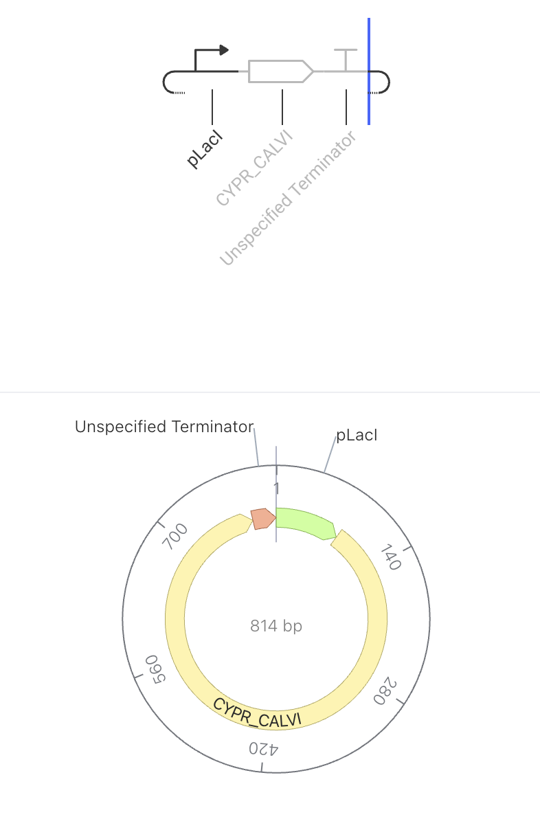
Construct 1: Rhodopsin Light-Sensitive Protein
new ideas from week 7 lec: modify it to make it like an activation function
How It Should Function
The promoter turns on, the rhodopsin protein gets made, and the terminator stops it. No feedback, no regulation — just expression.
The pLacI promoter drives constitutive expression of CYPR_CALVI, a light-sensitive rhodopsin protein. When the promoter is active, the cell continuously produces the rhodopsin protein. Because there is no feedback or regulation, protein levels are expected to rise steadily in the simulator. Rhodopsins are membrane proteins that respond to light, making them useful for optogenetic applications — controlling cell behavior using light.
Construct Image
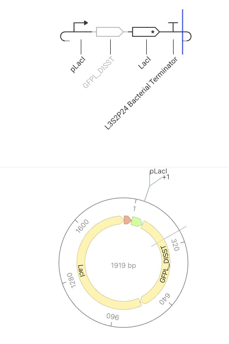
Construct 2: Negative Feedback Loop
How It Should Function
This circuit makes a glowing protein (GFP) AND a repressor at the same time. The repressor builds up and eventually turns the whole circuit off. The pLacI promoter drives simultaneous expression of both GFPL_DISST (green fluorescent protein) and LacI repressor. As more LacI accumulates in the cell, it begins to bind to and repress the pLacI promoter — slowing down production of both GFP and itself. This negative feedback loop acts as an auto-regulator: GFP levels rise initially, then stabilize or decline as LacI repression kicks in. The expected simulator output is a rise-then-plateau curve for GFP concentration.
Construct Image
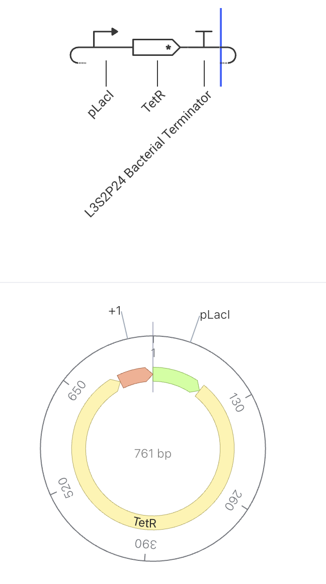
Construct 3: Toggle Switch
How It Should Function
This construct makes a repressor (TetR) that silences the other half of the switch. The two halves silence each other, so the cell can only be in one state at a time. This construct is one half of a classic bistable toggle switch. When pLacI is active, TetR is produced, which represses the pTet promoter in a paired construct. That paired construct produces LacI, which would repress pLacI. Because each side silences the other, the system locks into one of two stable states.
State 1 (TetR wins): pLacI ON → TetR high → pTet OFF → LacI low → pLacI stays ON
State 2 (LacI wins): pTet ON → LacI high → pLacI OFF → TetR low → pTet stays ON
Construct Image
Week 7 HW: Genetic Circuits Part II
Part 1. Intracellular Artificial Neural Networks
Q1. Advantages of IANNs over Traditional Boolean Genetic Circuits
A traditional genetic circuit works like a panel of on‑off light switches. Each gene is either fully expressed or completely silent, and the circuit’s output is a strict Boolean function of those binary inputs. An IANN, by contrast, behaves more like a set of dimmer switches connected through a mixing board. Each input can take any value within a continuous range, the connections have adjustable weights, and the final output is a smooth, graded signal instead of a hard 0 or 1.
This difference brings several benefits. Because IANNs are built from sequestrons that process signals in the analog domain, they can represent and compute with concentrations across a wide dynamic range. Boolean circuits squeeze all that richness into just two bins, but IANNs preserve it. A large enough IANN can in principle approximate any input‑output function, which is the biological version of the universal approximation theorem from machine learning. IANNs are also compact and scalable. Instead of layering many different logic gates, each with its own set of genetic parts, they use a single repeatable building block called a sequestron. The weights are set simply by adjusting DNA concentrations, so adding complexity means adding more copies of the same module rather than inventing new gate designs. Tuning the weights is like turning knobs on a mixing board: you change the ratio of plasmids, and the circuit’s behavior changes without needing to redesign any genetic parts. Finally, IANNs degrade gracefully. A small disturbance in the input causes only a small change in the output. Boolean circuits, on the other hand, can flip from the correct answer to the wrong one because of a tiny fluctuation near the switching threshold.
Q2. Applications
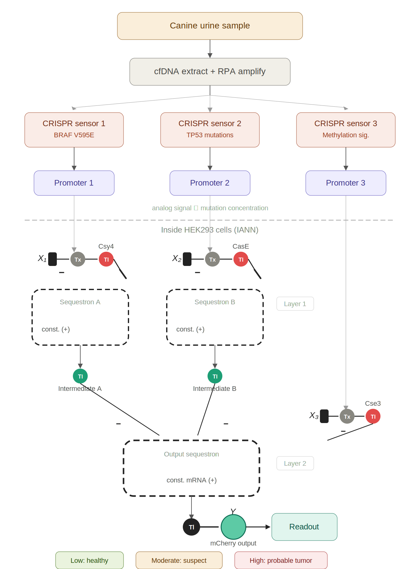
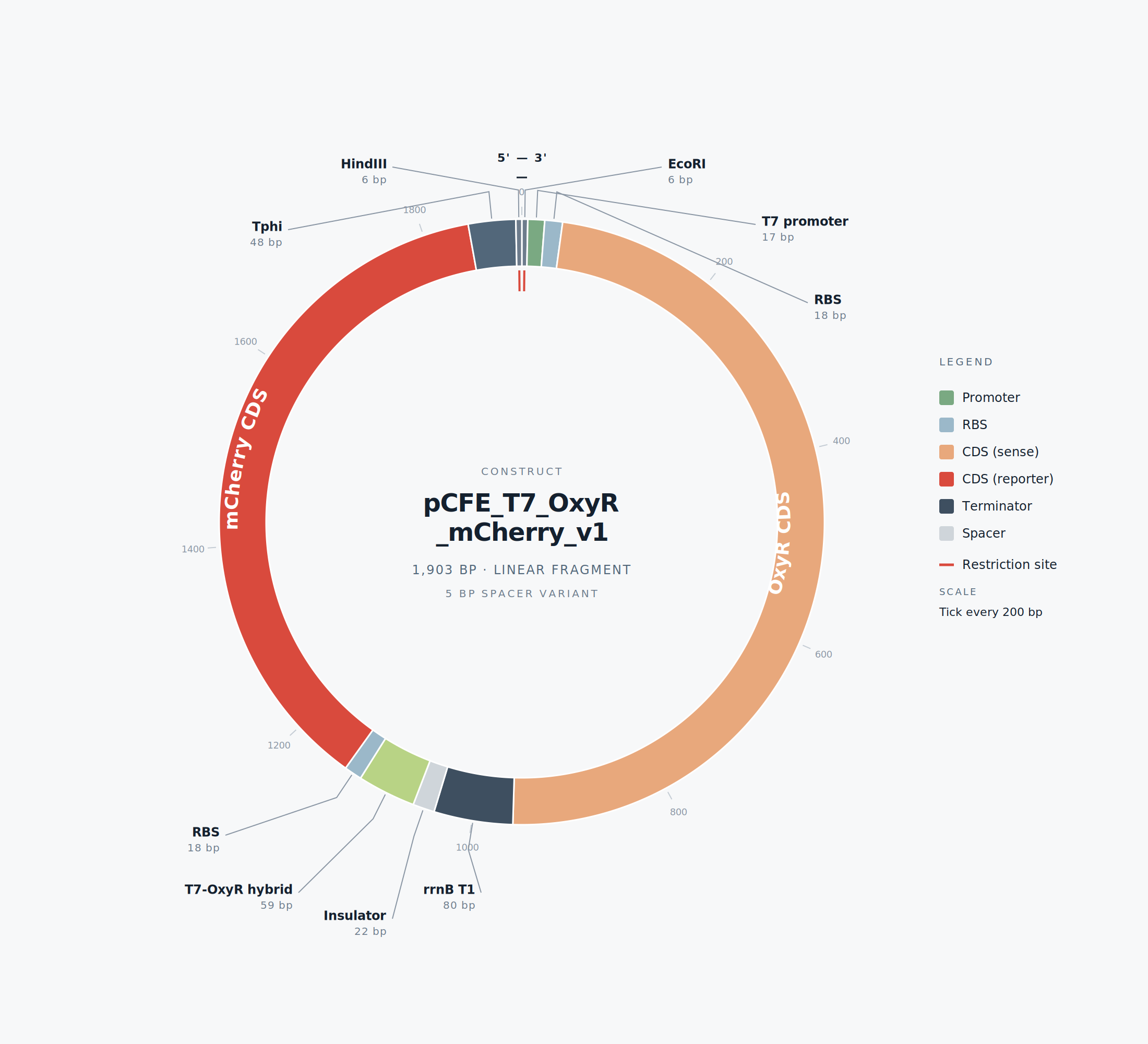
IANN could be designed to detect early tumor urinary tumor DNA (utDNA) in dogs by using CRISPR‑based DNA sensors that convert the presence of tumor‑specific mutations into transcriptional inputs for the IANN.
Pre-processing (in vitro): Three CRISPR-Cas13a sensors, each with mutation-specific crRNAs, detect BRAF V595E, TP53 mutations, and aberrant methylation in urine cfDNA. The collateral cleavage activity de-represses synthetic promoters proportionally to how much mutant DNA is present — converting molecular detection into analog transcriptional signals.
Computation (in vivo, HEK293 cells): A two-layer IANN built from sequestrons receives those three graded promoter signals as endoribonuclease inputs. Layer 1 integrates the BRAF and TP53 channels; Layer 2 combines Layer 1’s output with the methylation signal to produce a final weighted decision.
Output: mCherry fluorescence intensity acts as a continuous “cancer probability score” — low for healthy, moderate for single-mutation/early-stage, high for multi-mutation/advanced disease.
The analogy throughout is a team of sniffer dogs reporting to a handler — each dog gives a graded intensity signal for its specific scent (mutation), and the handler weighs them all to decide whether to raise the alarm.
The limitations section covers the real practical hurdles: sensitivity floor of CRISPR sensors for dilute utDNA, the sensor-to-cell interface challenge, transfection variability, the 650 ng DNA budget, temporal lag, incomplete mutation panels, gaps in canine methylome data, and lack of tissue-of-origin discrimination.
CRISPR-to-IANN canine utDNA detection system
Figure 1: Early canine tumor detection via CRISPR-to-IANN biosensor. Urine cfDNA is amplified and split across three CRISPR-Cas13a sensors targeting BRAF V595E, TP53 mutations, and methylation signatures. Each sensor de-represses a promoter proportionally to mutant utDNA concentration. Inside HEK293 cells, these analog signals feed a two-layer IANN built from sequestrons. The mCherry fluorescence output serves as a continuous cancer probability score.
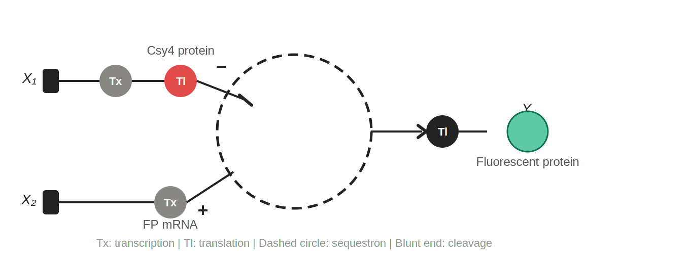
Q3 Single-layer intracellular perceptron
Figure 2: Single-layer intracellular perceptron. X₁ is DNA encoding the Csy4 endoribonuclease; X₂ is DNA encoding a fluorescent protein whose mRNA is regulated by Csy4. Tx: transcription; Tl: translation. The dashed circle represents the sequestron, where Csy4 (−) cleaves the fluorescent protein mRNA (+), and surviving mRNA is translated into the output Y.
Part 2. Fungal Materials
1.What are some examples of existing fungal materials and what are they used for? What are their advantages and disadvantages over traditional counterparts?
Mycelium packaging, such as Ecovative’s Mushroom Packaging, is made by growing mycelium on agricultural waste inside a mold. After a few days the material is heat‑killed and dried, producing a rigid, lightweight foam that can replace Styrofoam for protective packaging. It is completely biodegradable, grows on waste feedstocks, and uses little energy to manufacture. However, it has lower compressive strength than Styrofoam, is sensitive to moisture, and is slower to produce at scale.
Mycelium leather, like Bolt Threads’ Mylo and MycoWorks’ Reishi, is grown as a pure sheet in controlled fermentation, then tanned and finished much like animal leather. It is used in fashion and accessories. It requires no animal farming and has a much lower water and land footprint, and its thickness and texture can be tuned. On the downside, it is still expensive at small scale, its durability and aging properties are still being improved, and it needs chemical post‑processing to match the flexibility of animal leather.
Mycelium‑based building insulation is grown on straw or wood shavings and can be used as thermal and acoustic panels. It has heat insulation similar to synthetic foams and is naturally fire‑retardant. It is non‑toxic, sequesters carbon, and resists fire better than petroleum‑based foams. But it is not strong enough for structural uses and can degrade if it gets wet.
Mycoprotein foods like Quorn and Meati come from fermenting filamentous fungi to make high‑protein, fibrous biomass that feels like meat. These products are high in protein, have a complete amino acid profile, and produce far fewer greenhouse gases than animal farming. Still, some people are allergic, the feedstocks are sugar‑based, and the taste and texture are not yet exactly the same as real meat.
Mycelium automotive parts were explored by Ford and Ecovative for interior pieces like dashboards, door panels, and seat cushions, taking advantage of the material’s sound absorption and impact resistance. They are lightweight, need no adhesive because the mycelium acts as the binder, and can be composted at the end of their life. However, they are sensitive to water, there is not yet much data on long‑term durability, and they are not yet cost‑competitive with synthetic foams at automotive scale.
2. What might you want to genetically engineer fungi to do and why? What are the advantages of doing synthetic biology in fungi as opposed to bacteria?
Bacteria are like bicycles: fast, simple, and cheap, good for making small proteins and simple chemicals. Fungi are like trucks. They are eukaryotes, so they have the cellular machinery to fold complex proteins, add post‑translational modifications, and build intricate three‑dimensional structures that bacteria simply cannot make. One can make mycelium materials that are naturally stronger, more flexible, or more water‑resistant without needing chemical post‑processing. You can also make fungi produce high‑value proteins while they are growing. They could secrete antimicrobial peptides, fire‑retardant proteins, or pigments directly into the material, creating functional composites in a single step. You could create self‑healing materials by engineering dormant spores into dried mycelium composites that reactivate when water enters a crack, similar to how skin heals. You could also enhance bioremediation by engineering white‑rot fungi to produce extra versions of the enzymes that break down plastics, pesticides, or industrial dyes.
Compared to bacteria, fungi have many advantages for synthetic biology. They fold and modify proteins correctly because they have an endoplasmic reticulum and Golgi apparatus, which bacteria lack. Their hyphal growth lets them naturally form sheets, foams, and composites; bacteria only grow as single cells in liquid. Fungi can grow on cheap, unprocessed plant waste because they secrete powerful enzymes to break down cellulose and lignin, while most bacteria need processed sugars. Their eukaryotic compartments let them keep toxic intermediates separate and run incompatible pathways at the same time, which helps them make complex natural products. Genetic tools like CRISPR‑Cas9, promoter libraries, and selectable markers are now well developed in model fungi, making engineering much easier. And because fungi are multicellular, they can form different tissue types such as aerial hyphae or fruiting bodies, opening up possibilities for spatial organization and layered material architectures that are impossible with single‑celled bacteria.
Week 9 HW: Cell Free Systems
##Part 1
1.Advantages of Cell-Free Over In Vivo Expression
Cell-free protein synthesis (CFPS) removes the cell as a “black box” and allows you directly control and observe every variable in real time: pH, redox potential, ionic strength, and cofactor concentration.
2.Main Components and Their Roles
Component
Role
Cell extract
Provides ribosomes, tRNA, synthetases, chaperones, and machinery
DNA/mRNA template
Encodes the target protein (plasmid or linear)
RNA polymerase
Transcribes DNA → mRNA (T7 RNAP is most common)
Amino acids
Raw building blocks for translation
Energy system
Supplies and recycles ATP/GTP to power translation
Salts and buffer
Maintains pH (~7.5) and ionic strength (Mg²⁺, K⁺ critical)
Additives
Chaperones, detergents, etc., added based on target needs
3.Energy Provision and ATP Regeneration
Translation is enormously ATP-hungry: every peptide bond costs ~4 high-energy phosphate bonds. In a tube, the initial ATP pool depletes within 30–60 minutes, stalling ribosomes and collapsing yield.
Phosphocreatine / Creatine Kinase System
ADP + phosphocreatine → ATP + creatine (catalyzed by creatine kinase)
Add phosphocreatine (~20 mM) and creatine kinase (~0.5 mg/mL).
Extends productive reaction time from ~1 hour to 3–6 hours.
Alternative: Maltose/maltodextrin system — a multi-enzyme cascade mimicking glycolysis, cheaper for large-scale reactions.
4.Prokaryotic vs. Eukaryotic Cell-Free Systems
Feature
Prokaryotic (E. coli)
Eukaryotic (wheat germ / CHO)
Post-translational mods
None
Glycosylation, phosphorylation, etc.
Cost
Low
High
Yield
High
Moderate
Best for
Simple cytosolic proteins
Mammalian proteins, antibodies, GPCRs
Prokaryotic Choice — T7 RNA Polymerase: Straightforward cytosolic protein, no PTMs needed, high yield required.
Eukaryotic Choice — Erythropoietin (EPO): Requires N-linked glycosylation for proper folding. A prokaryotic system would produce misfolded, inactive protein.
Designing Cell-Free Expression of a Membrane Protein
Membrane proteins are hydrophobic — without a lipid bilayer, they aggregate instantly.
Three Solubilization Strategies
Detergent micelles (DDM, digitonin) — Simplest; add directly to reaction.
Nanodiscs — Pre-assembled lipid bilayer discs; co-translate so protein inserts immediately.
Liposomes — Lipid vesicles that capture the protein as it emerges from the ribosome.
##Part 2 Synthetic Minimal Cell: Gut Microbiome Inflammation Sensor
1. Function
1a. What It Does — Input and Output
A liposome-based synthetic cell that detects elevated reactive oxygen species (ROS) in the gut lumen — a molecular signature of intestinal inflammation — and responds by producing and releasing butyrate, a short-chain fatty acid that suppresses NF-κB signaling and restores epithelial barrier integrity.
Feature
Description
Input
Hydrogen peroxide ($H_2O_2$) and superoxide — ROS elevated during gut inflammation (IBD, Crohn’s, colitis)
Output
Butyrate (butanoic acid) — anti-inflammatory metabolite that feeds colonocytes and suppresses immune activation
Analogy: Think of it like a smoke detector hardwired to a fire sprinkler — the same signal that trips the alarm also triggers the response, with no human intervention needed. The synthetic cell is silent in a healthy gut and active only when and where inflammation occurs.
1b. Could Cell-Free Tx/Tl Alone Do This Without Encapsulation?
No. There are three primary reasons:
Directionality: Without a membrane boundary, butyrate produced freely in solution would diffuse away immediately with no directional delivery to the epithelium.
Protection: The ROS-sensing gene circuit would be exposed to gut proteases and nucleases, degrading within minutes.
Threshold Control: There is no mechanism for threshold-gated release — the entire reaction would fire at once rather than responding proportionally to local ROS concentration.
1c. Could a Genetically Modified Natural Cell Do This?
Partially — but with serious limitations compared to a synthetic liposome:
Feature
Engineered Bacterium
Synthetic Liposome Cell
ROS sensing
Possible via OxyR regulon
Possible via OxyR-driven promoter
Butyrate synthesis
Yes — multiple chassis
Yes — encapsulated enzyme pathway
Immune clearance
High — triggers innate immunity
Minimal — PEGylated lipids are inert
Replication control
Requires auxotrophy kill switch
Non-replicating by design
Gene Transfer
Risk of horizontal transfer
Zero risk
Regulatory path
Extremely difficult (GMO in gut)
More tractable as a drug delivery device
1d. Desired Outcome
A synthetic cell administered orally (enteric-coated capsule) that survives transit to the colon, remains transcriptionally silent in healthy tissue, and activates butyrate synthesis specifically at inflamed foci where $H_2O_2$ exceeds threshold (~50 µM).
2. Component Design
2a. Membrane Composition
The membrane is designed to survive the harsh gut environment (low pH, bile salts) while remaining functional at 37°C.
Lipid
Role
Mol%
DPPC
High-Tm structural lipid; bile salt resistance
40%
POPE
Supports protein insertion; reduces curvature stress
25%
Cholesterol
Rigidifies bilayer; reduces permeability
25%
DSPE-PEG2000
PEG brush layer; prevents immune recognition
10%
2b. Encapsulated Contents
The “cytoplasm” of the synthetic cell contains the following:
Tx/Tl Machinery:E. coli cell-free extract (ribosomes, tRNA, chaperones), T7 RNA Polymerase, and the OxyR-responsive promoter plasmid.
Pre-loaded Enzymes: Acetyl-CoA acetyltransferase (ThlA) for fast initial response.
Small Molecules: Acetyl-CoA (2 mM), Phosphocreatine (20 mM) + creatine kinase (0.5 mg/mL), all 20 amino acids (5 mM each), and essential cofactors (NAD⁺/NADH, CoA).
2c. Tx/Tl System Origin: Bacterial (E. coli)
A prokaryotic system is preferred because the OxyR transcription factor and the butyrate synthesis enzymes (from Clostridium) are natively bacterial. No complex post-translational modifications (PTMs) are required, making the high-yield E. coli extract the most efficient choice.
2d. Communication with the Environment
Sensing (IN — Passive): $H_2O_2$ crosses lipid bilayers freely via passive diffusion. Inside, it oxidizes OxyR, switching it from a repressor to an activator.
Secretion (OUT — Active): We express VDAC-1 (voltage-dependent anion channel 1). While butyrate is anionic at physiological pH, the expressed VDAC-1 pores permit rapid efflux.
3. Experimental Details
3a. Complete Genes and Lipids
Gene
Organism
Role
oxyR
E. coli K-12
ROS-activated transcription factor
thlA
C. acetobutylicum
Step 1: 2 acetyl-CoA → acetoacetyl-CoA
hbd
C. acetobutylicum
Step 2: → 3-hydroxybutyryl-CoA
crt
C. acetobutylicum
Step 3: → crotonyl-CoA
bcd/etfAB
C. acetobutylicum
Step 4: → butyryl-CoA
ptb/buk
C. acetobutylicum
Steps 5–6: → butyrate
VDAC1
H. sapiens
Membrane pore for butyrate efflux
3b. Measuring System Function
Validation is performed through a tiered strategy:
Tier 1: ROS-responsive expression: Use a GFP reporter to confirm the OxyR circuit activates at the ~50 µM $H_2O_2$ threshold.
Tier 2: Butyrate synthesis: Quantify butyrate production in bulk extract using GC-MS or enzymatic assays.
Tier 3: Pore function: Use ANTS/DPX dye efflux assays to confirm VDAC-1 correctly inserts into the liposome membrane.
Tier 4: Integrated function: Measure butyrate secretion from encapsulated cells in simulated healthy (5 µM $H_2O_2$) vs. inflamed (100 µM $H_2O_2$) conditions.
Tier 5: Bioactivity: Apply the output to Caco-2 cells and measure the reduction in inflammatory markers (IL-8/NF-κB).
##Part 3. Aura-Weave (Smart Medical Wearables)
1. One-Sentence Summary Pitch
Aura-Weave is a smart, disposable textile liner for adult incontinence garments that uses freeze-dried cell-free extracts to seamlessly detect and visually report urinary tract infections (UTIs) by changing color when exposed to infected urine.
2. How the Idea Works in Detail
The Aura-Weave liner features a middle diagnostic layer composed of a highly absorbent cellulose matrix (similar to filter paper). This matrix is pre-loaded with a lyophilized (freeze-dried) cell-free extract (CFE), specific engineered DNA circuits, and pH buffers.
The Mechanism:
Dormancy: The system remains completely inactive on the shelf in its dry state.
Activation: When the wearer voids urine, the warm liquid acts as the natural rehydration trigger, “booting up” the biological transcription and translation machinery.
Detection: If specific UTI biomarkers are present—such as nitrites, leukocyte esterase, or bacterial quorum-sensing molecules—the genetic circuit is triggered.
Visual Output: The circuit drives the rapid expression of a vibrant chromoprotein (like AmilCP). Within 45 to 60 minutes, a clear blue warning symbol permeates to the outer visible edge of the textile.
Visual Indicator: A blue symbol or color change alerts the caregiver immediately without requiring a manual diagnostic test.
3. Societal Challenge and Market Need
This addresses the “silent crisis” of UTIs in elderly, bedridden, and cognitively impaired populations (such as those with Alzheimer’s or dementia).
Communication Barriers: These patients often cannot communicate early symptoms like pain or urgency, leading to delayed diagnosis.
Medical Risks: Late-stage UTIs frequently progress to severe kidney infections, sepsis, and costly hospitalizations.
Non-Invasive Monitoring: Aura-Weave eliminates the difficult, messy, and stress-inducing process of collecting a clean urine sample from an uncooperative patient, allowing for continuous, passive health monitoring in nursing homes and home-care settings.
4. Addressing Cell-Free Limitations
Limitation
Aura-Weave Strategy
Water Activation
The Built-in Trigger: In this context, rehydration is a feature. The CFE stays inactive until the exact moment the patient urinates, ensuring the test only runs when a sample is provided.
Stability
Sugar Matrix Stabilization: To ensure a shelf life of over a year, the CFE and DNA are co-lyophilized with a stabilizing sugar (trehalose) and a strong buffer (HEPES), locking proteins in a stable, glass-like state at room temperature.
One-Time Use
Lifecycle Alignment: Incontinence liners are inherently single-use. The biological sensor’s lifecycle perfectly matches the textile’s lifecycle; once soiled and read, the garment is safely discarded.
Storage Requirements: Room temperature (stabilized via Trehalose).
##Part 4
The Challenge: Current missions detect “bricks” (organic molecules) but not “factories” (active life).
Strategy: Use FD-CF systems to detect ATP Synthesis and 16S rRNA genes.
Reasoning: Only active biology synthesizes ATP; abiotic chemistry (like meteorites) might have organics but no coordinated metabolism.
Experimental Plan: Compare Mars simulant spiked with extremophiles against sterile simulant and abiotic meteorite extracts.
Week10 HW: Imaging and Measurement
What to measure: Identity, mass, purity, and post-translational modifications of the target protein; concentration of a biomarker; oligomeric state.
How:
Intact mass by LC-MS (QTof) → confirms overall MW and detects unexpected modifications.
Peptide mapping by tryptic digest + LC-MS/MS → confirms primary sequence and identifies PTM sites.
Native MS / CDMS → reveals folded state and oligomeric assembly.
SDS-PAGE / Western blot → quick purity and identity check before MS.
UV-Vis (A280) → concentration.
Part I — Molecular Weight of Intact eGFP
Q1. Theoretical MW from sequence
Sequence length: 247 residues (includes LE linker + HHHHHH His-tag).
Calculated average MW ≈ 28,006.6 Da (~28 kDa).
Analogy: counting MW from sequence is like weighing a train by summing the weight of each car — every amino acid adds its known “car weight” minus one water molecule per peptide bond.
Q2. Deconvolution from Figure 1
Selected adjacent peaks (denatured envelope): m/z = 933.7148 and m/z = 903.7148.
That is ~3,200 ppm error — excellent for intact-protein QTof analysis.
Q3. Charge state of the zoomed-in peak (~1473 m/z region)
No, the charge state cannot be confidently assigned from the zoom. Reason: the zoomed peak shows partially resolved features, but at 30,000 resolution on a ~28 kDa protein the isotope envelope is not baseline-resolved — adjacent isotope peaks are not separated by a clean 1/z spacing you can read off. To assign charge from isotope spacing you need resolution high enough to see individual ¹²C/¹³C isotope peaks (≥60,000–100,000 for a protein this size, ideally on an Orbitrap or FT-ICR).
Analogy: trying to count the steps of a staircase from far away — if your camera (resolution) isn’t sharp enough, the steps blur into a ramp.
Part II — Native vs Denatured (Secondary/Tertiary)
Q1. What changes when a protein unfolds, and how MS sees it
Native (folded): the protein is compact, so only a few surface residues are accessible to protons during electrospray → it picks up few charges → peaks appear at high m/z, in a narrow charge envelope (e.g., Figure 2 bottom: ~2500–3000 m/z, only ~2–3 charge states).
Denatured (unfolded): the chain is extended, exposing every basic residue (K, R, H, N-terminus) to protonation → it picks up many charges → peaks span a broad envelope at low m/z (Figure 2 top: ~700–1500 m/z, many charge states).
The mass is the same — only the charge distribution shifts. MS reads the protein’s “shape” indirectly through how many protons it carries.
Analogy: a folded origami crane has only a few outer surfaces to stick stickers (charges) on; unfold it into a flat sheet and you can stick stickers everywhere. The paper hasn’t changed weight, but the sticker count tells you the shape.
Q2. Charge state at ~2800 m/z (native)
Inset isotope spacing in Figure 3: peaks at 2544.4885, 2544.5801, 2544.6719, 2544.7637, 2544.8552, 2545.0388 → spacing ≈ 0.092 m/z.
In silico digest (no missed cleavages, cleavage after K/R unless followed by P): 27 peptides total. PeptideMass with mass cutoff ≥500 Da returns ~17 peptides (filters out very small fragments like TR, QK, IR, single R).
Q3. Chromatographic peaks in TIC (0.5–6 min, >10% abundance)
From Figure 5a, counting peaks above 10% relative intensity: ~15–17 peaks (the most prominent at 0.43, 0.61, 0.79, 1.20, 1.43, 1.80, 1.85, 1.93, 2.17, 2.26, 2.54, 2.78, 3.27, 3.53, 3.59, 3.70, 4.30, 4.48, 4.64, 4.87, 5.06, 5.43, 6.12, 6.50, 6.64, 6.73 — about 15 of these clearly exceed 10%).
Q4. Does peak count match predicted peptides?
The TIC shows fewer peaks than predicted (~15 visible vs 27 predicted). Reasons:
Very small peptides (TR, QK, IR, R, NGIK) are below the MS detection range or wash out in the dead volume.
Some peptides co-elute (overlap in retention time).
Some hydrophilic peptides aren’t retained on C18 reverse-phase column.
Excellent accuracy (sub-10 ppm is standard for QTof).
Q7. Sequence coverage
From Figure 6: 88% of the eGFP sequence is confirmed by peptide mapping.
Bonus Q8. Sequence from fragmentation (Figure 5c)
Fragment masses (122.07, 214.09, 388.22, 501.31, 602.35, 537.25, 774.41, 903.44, 1050.52) match the b- and y-ion series for FEGDTLVNR. Key y-ions: y1 (R) = 175.12, y2 (NR) = 289.16, y7 (GDTLVNR), and the immonium ion at 122.07 corresponds to F (phenylalanine immonium). Confirms FEGDTLVNR.
Bonus Q9. Does the data confirm eGFP?
Yes. 88% sequence coverage + a confirmed peptide (FEGDTLVNR) with <10 ppm mass error + matching fragmentation pattern is strong identification. The unobserved 12% is typical (very short peptides or unretained hydrophilic peptides) and doesn’t undermine the ID.
Analogy: it’s like recognizing a friend from 88% of their face uncovered — you don’t need every feature, you just need enough unique landmarks.
Part IV — KLH Oligomers (CDMS)
Using subunit masses: 7FU = 340 kDa, 8FU = 400 kDa, and “Decamer” = 10 subunits.
Oligomer
Composition
Expected mass
Peak in Figure 7
7FU Decamer
10 × 340 kDa
3.4 MDa
peak at 3.4 MDa
8FU Didecamer
20 × 400 kDa
8.0 MDa
peak at ~7.52 MDa (close to 8.0; some mass loss possible)
8FU 3-Decamer
30 × 400 kDa
12.0 MDa
peak at 12.67 MDa
8FU 4-Decamer
40 × 400 kDa
16.0 MDa
peak around ~16 MDa (small/absent)
The prominent 4.013 MDa peak is likely an 8FU decamer (10 × 400 = 4.0 MDa). The 0.1982, 0.79, 1.52 peaks are sub-decameric assemblies/free subunits.
Analogy: CDMS measures each particle individually — like weighing each LEGO build that walks past on a conveyor belt, instead of melting them all and weighing the slag. You see exactly which assemblies exist.
Part V — Validate GFP?
Theoretical
Observed (Intact LC-MS)
PPM Mass Error
Molecular weight (kDa)
28.007
~28.097 (from deconvolution of Figure 1)
~3,200 ppm (0.32%)
The observed intact mass agrees with the theoretical mass of eGFP+LE+His₆ to within ~0.3%. Combined with 88% peptide map coverage and confirmed FEGDTLVNR fragmentation → yes, this is eGFP.
Week11 HW: BIOPRODUCTION AND CLOUD LABS
Unfortunately I was away at CHI 2026 during the contribution window, so I didn’t get to commit a pixel in time.
Part B – Cell-Free Protein Synthesis
B1. Role of each component
E. coli Lysate
BL21 (DE3) Star Lysate (with T7 RNAP): The “factory floor” – a crude cytoplasmic extract carrying ribosomes, tRNAs, aminoacyl-tRNA synthetases, translation factors, and the T7 RNA polymerase needed to transcribe T7-promoter templates. The DE3 Star background also lacks RNase E activity, so mRNAs last longer.
Salts / Buffer
Potassium Glutamate: Main osmolyte and K+ source for ribosome function; glutamate (unlike chloride) doesn’t inhibit translation.
HEPES-KOH pH 7.5: pH buffer – holds the reaction near physiological pH so enzymes work and chromophores fold correctly.
Magnesium Glutamate: Mg2+ is essential cofactor for RNAP, ribosome assembly, and every nucleotide-binding enzyme. Glutamate counter-ion again, for the same reason as K+.
Potassium phosphate (mono/dibasic, 1.6:1): Phosphate buffer + Pi source. Pi is recycled into NTPs and into the energy regeneration loop.
Energy / Nucleotide System (NMP-Ribose system)
Ribose: Carbon backbone for nucleotide regeneration; cellular enzymes in the lysate convert ribose + NMPs into NTPs.
Glucose: Primary energy source – glycolysis in the lysate regenerates ATP from ADP, powering everything else.
AMP, CMP, GMP, UMP: Cheap nucleotide monophosphates supplied as precursors; lysate kinases phosphorylate them up to NTPs as needed (this is why NMP-Ribose is cheaper than buying NTPs directly).
Guanine: Free base that lysate enzymes salvage into GMP/GDP/GTP – this is the workaround for the missing GMP in the mix (see B3).
Translation Mix (Amino Acids)
17 Amino Acid Mix: The protein building blocks. Tyrosine and cysteine are supplied separately because they have solubility/oxidation quirks.
Tyrosine (pH 12): Tyrosine is poorly soluble at neutral pH, so it’s prepared in a strong alkaline stock and added separately.
Cysteine: Highly reactive thiol – prone to oxidation and disulfide formation, so kept separate and added fresh.
Additives
Nicotinamide: Precursor for NAD+/NADH – needed by glycolysis (GAPDH step) to keep the energy regeneration cycle running.
Backfill
Nuclease-Free Water: Brings the reaction to volume without introducing RNases that would chew up the mRNA.
Analogy: the cell-free reaction is a kitchen with the chefs (ribosomes, polymerase), the recipes (DNA template), and an inventory system (energy regeneration). The 20-h mix is set up so the kitchen doesn’t run out of energy after one hour – instead of pre-cooked NTPs, it ships in flour (ribose) and grain (NMPs) and bakes its own NTPs continuously.
B2. PEP-NTP vs NMP-Ribose master mix – main differences
The PEP-NTP mix is a sprint: it supplies finished NTPs directly plus PEP (phosphoenolpyruvate) as a high-energy phosphate donor, giving immediate energy and transcription for fast 1-hour reactions, but it’s expensive and burns out as PEP depletes. The NMP-Ribose mix is a marathon: it supplies cheap NMP precursors + ribose + glucose so the lysate’s own enzymes regenerate NTPs and ATP continuously, sustaining transcription/translation for 20 hours at much lower cost.
Analogy: PEP-NTP is buying a pre-charged battery; NMP-Ribose is installing a slow-trickle solar panel. The battery is faster at first but it runs out – the panel keeps producing as long as the sun (glucose) is shining.
B3. Bonus – Transcription without GMP, only Guanine
E. coli lysates retain the purine salvage pathway. Enzymes such as HGPRT (hypoxanthine-guanine phosphoribosyltransferase) convert free guanine + PRPP (which the lysate makes from ribose and ATP) into GMP, and then nucleotide kinases (GMK, NDK) phosphorylate GMP -> GDP -> GTP. So guanine + ribose effectively replaces GMP at a fraction of the cost.
Analogy: you don’t buy bread if you have flour and a baker. The lysate has the baker (HGPRT + kinases) and the flour (ribose), so guanine is enough.
Part C – Planning the Global Experiment
C1. One key biophysical property of each FP affecting cell-free readout
sfGFP – Fast, robust folding even under stress. sfGFP was engineered specifically to fold and mature quickly in conditions where regular GFP fails (heterologous expression, fusion tags). In cell-free, this means it lights up earliest of the green channel and is a forgiving “always works” baseline. Like GFP family, it needs O2 for chromophore maturation (oxidation step), but its maturation is fast (~14 min in vivo).
mRFP1 – Slow maturation and stepwise blue->red intermediate. mRFP1 (the original DsRed-derived monomer) matures over hours via a blue/green intermediate, so 1-hour reactions barely capture any red signal – a 36-h incubation is essentially required to see full red. Also O2-dependent (extra oxidation step compared to GFP).
mKO2 – Orange FP with moderate maturation, pH-stable. mKO2 (from Fungia coral) has good photostability and a relatively low pKa (~5.5), so it tolerates the slight pH drift cell-free reactions experience as glucose ferments to lactate/acetate. Maturation slower than GFP-class but faster than DsRed-derived reds.
mTurquoise2 – High quantum yield, but pKa ~3.1 means very acid-resistant; sensitive to chloride. Probably the brightest cyan available, with QY ~0.93. It folds well in E. coli lysates. Its CFP-class chromophore is insensitive to acidification, so it’s a great choice if the long-incubation pH drops. Like GFP, needs O2.
mScarlet-I – Fastest-maturing monomeric red (~31 min in yeast), but moderate acid sensitivity (pKa ~5.4). This makes it the best red for short or pH-stable reactions; if pH drifts below ~6, signal drops noticeably.
Electra2 – Blue FP derived from mRuby3, monomeric, bright, with a chromophore that doesn’t require O2 for maturation in the same way GFP does (BFPs of this class form their chromophore via a different cyclization route). Designed for live-cell intracellular brightness, which translates well to cell-free. Spectral non-overlap with the green/red FPs makes it ideal for the multi-color canvas.
C2. Hypothesis – one reagent adjustment to improve a specific property
Protein: mRFP1
Reagent(s) to adjust: increase dissolved O2 (looser cap / higher headspace / pre-oxygenated buffer) and add supplemental FAD (~1 uM).
Expected effect: mRFP1 maturation includes an O2-dependent oxidation step that’s rate-limiting in sealed cell-free wells, where O2 depletes fast. Increasing O2 availability should accelerate red chromophore formation and raise final fluorescence at 36 h without changing protein yield. FAD has been shown to assist DsRed-family oxidative maturation. Predicted endpoint: >=1.5x fluorescence vs default well.
Alternative hypothesis (mScarlet-I): Increase HEPES buffer concentration from 45 mM -> 80 mM to prevent pH drift below mScarlet-I’s pKa (~5.4) over 36 h. Expected effect: maintain protonation state of the chromophore, preserve fluorescence quantum yield, and prevent late-incubation signal decay.
Analogy: in photography terms, this is choosing the right film for the lighting. mTurquoise2 is high-ISO film (works in any light/pH), mRFP1 is a film that needs long exposure (slow maturation), mScarlet-I is film that gets fogged by acid in the developer (acid-sensitive) – so you adjust the chemistry (buffer, O2, time) to suit the film.
Part B — Cell-Free Protein Synthesis B1. Role of each reagent (20 h NMP-Ribose-Glucose mix) Component Role in the reaction BL21 (DE3) Star lysate Source of ribosomes, tRNAs, aminoacyl-tRNA synthetases, and other translation machinery. (DE3) carries T7 RNAP for transcription; Star = reduced RNase E -> mRNA more stable. Potassium glutamate Dominant monovalent cation, mimics cytoplasmic ionic environment, stabilizes ribosome conformation. Glutamate (vs Cl-) doesn’t inhibit translation. HEPES-KOH pH 7.5 Zwitterionic buffer holds pH near physiological — keeps T7 RNAP and ribosomes active. Magnesium glutamate Mg 2+ cofactor for ribosome assembly, T7 RNAP, and aminoacyl-tRNA synthetases. Concentration is highly tunable — too low halts translation, too high promotes misincorporation. K-phosphate mono/dibasic Secondary pH buffer + phosphate pool for nucleotide kinase reactions (NMP -> NDP -> NTP). Ribose Feeds the salvage pathway: ribokinase -> ribose-5-P -> PRPP, which combines with free bases to form NMPs. Also a slow-burning energy substrate. Glucose Carbon source for glycolysis -> continuous ATP regeneration (sustained energy, unlike PEP which burns fast). AMP / CMP / UMP NMP precursors. Cellular kinases phosphorylate them to NTPs in situ -> slower ramp than feeding NTPs, but cheaper and less product-inhibition. GMP (0 mM here) Omitted in the 20 h mix; GTP is generated via the Guanine salvage path instead (see bonus). Guanine Substrate for HGPRT: Guanine + PRPP -> GMP + PPi. Cheaper than buying GMP directly. 17 amino acid mix Bulk substrate pool for translation (all proteinogenic AAs except Tyr and Cys, which need special handling). Tyrosine (pH 12) Added separately — Tyr has very low solubility at neutral pH and must be kept in alkaline solution until dilution. Cysteine Added separately — readily oxidizes to cystine (forms disulfides). Kept in its own tube to avoid inactivation before reaction start. Nicotinamide NAD+ precursor + inhibitor of NAD-degrading enzymes (NADases) in the lysate -> preserves the redox cofactor pool over the long incubation. Nuclease-free water Backfill to final volume; nuclease-free to protect the DNA template and mRNA. B2. PEP-NTP (1 h) vs NMP-Ribose-Glucose (20 h) The PEP-NTP mix feeds the reaction with finished NTPs and uses phosphoenolpyruvate as a high-energy ATP regenerator — fast, intense protein synthesis, but PEP is depleted within ~1 hour and the system burns out. The NMP-Ribose-Glucose mix instead supplies precursors (NMPs + ribose for PRPP, glucose for glycolytic ATP) and lets the lysate’s own kinases and salvage enzymes assemble NTPs on demand, giving a slower but sustained ramp that lasts 20+ hours. Cost-per-reaction is also much lower because cheap precursors replace expensive NTPs and PEP.
Week 6: Gibson Assembly Group members: Louisa Zhu, Shitong, Jasmin
Part 1 1. PCR Figure 1. PCR reaction setup tables for the Backbone DNA Fragment (top) and Color DNA Fragment (bottom), including reagent volumes for a 25 µL total reaction.
Overview In this lab, we designed two neuromorphic genetic circuits using the HTGAA 2026 Genetic Circuit Design Template and simulated their behavior using the Biocompiler-Predict tool. Both circuits are built from endoribonuclease-based sequestrons — the fundamental building blocks of intracellular artificial neural networks (IANNs) — and are intended for transfection into HEK293 cells via Lipofectamine 3000 and execution by an OT-2 liquid handling robot.
Subsections of Labs
Week 1 Lab: Pipetting
Pre-lab answers
Stock MS in g/mL
5 M × 532 g/mol = 2660 g/L = 2.66 g/mL
Serial dilution plan: 5 M → 100 µM
Total dilution = 50,000× → 2 steps.
Step
From → To
Factor
Take stock
+ dH₂O
Final vol
Pipette
1
5 M → 10 mM
500×
2 µL
998 µL
1000 µL
P2/P20 + P1000
2
10 mM → 100 µM
100×
10 µL
990 µL
1000 µL
P20 + P1000
Tubes: 1.5 mL Eppendorfs (volumes too large for PCR strips).
Final reaction (60 µL, MS at 40 µM, dye at 1×)
Reagent
Stock
Final
Volume
Loading dye
6×
1×
10 µL
MS
100 µM
40 µM
24 µL
dH₂O
—
—
26 µL
Total
60 µL
Why 100 µM intermediate instead of diluting straight to 40 µM? 100 µM is a clean serial-dilution endpoint (50,000× = 500× × 100×); 40 µM isn’t. The 100 µM tube also acts as a reusable stock for downstream reactions — error compounds with every extra dilution step, so fewer steps to a clean intermediate is better.
Part 1 — Mixing color (practice)
Followed protocol: tubes 1–3 single colors (500 µL each), tubes 4–6 mixed pairs (R+Y, Y+B, R+B). Two-step pipetting (200 + 20 µL) on tube 4 to practice tip changes.
Plating designs: Used 1–10 µL drops on a glass petri to build volume intuition. Drop diameter scales noticeably with volume — 1 µL drops are barely visible without backlight; 10 µL drops bead high enough to catch reflection.
Result
I pipetted the 甲骨文 (oracle bone script) of 马 — the Chinese character for horse — onto the plate to celebrate the Year of the Horse (2026). Oracle bone script is the earliest known form of Chinese writing, carved into ox scapulae and turtle plastrons during the Shang dynasty (~14th–11th c. BCE) for divination. The pictographic form of 马 still shows the horse’s mane, four legs, and tail.
Reference character (甲骨文 of 马)
My pipetted plate
Observations:
Drop size variability across the design = visible record of where my hand was steady vs. shaky.
Surface tension on bare glass keeps drops discrete — no spreading or merging unless they touched.
Part 2 — Serial dilution
Performed the two-step dilution per the table above. Mixed by pipetting up/down 3–4× after each addition. Marked tubes with target concentration.
Prepared the 60 µL final reaction. Loaded 20 µL into a pre-prepared gel well (bonus step) — went in cleanly without puncturing.
Week 11 Lab: Cloud Lab
Part B — Cell-Free Protein Synthesis
B1. Role of each reagent (20 h NMP-Ribose-Glucose mix)
Component
Role in the reaction
BL21 (DE3) Star lysate
Source of ribosomes, tRNAs, aminoacyl-tRNA synthetases, and other translation machinery. (DE3) carries T7 RNAP for transcription; Star = reduced RNase E -> mRNA more stable.
Zwitterionic buffer holds pH near physiological — keeps T7 RNAP and ribosomes active.
Magnesium glutamate
Mg 2+ cofactor for ribosome assembly, T7 RNAP, and aminoacyl-tRNA synthetases. Concentration is highly tunable — too low halts translation, too high promotes misincorporation.
K-phosphate mono/dibasic
Secondary pH buffer + phosphate pool for nucleotide kinase reactions (NMP -> NDP -> NTP).
Ribose
Feeds the salvage pathway: ribokinase -> ribose-5-P -> PRPP, which combines with free bases to form NMPs. Also a slow-burning energy substrate.
Glucose
Carbon source for glycolysis -> continuous ATP regeneration (sustained energy, unlike PEP which burns fast).
AMP / CMP / UMP
NMP precursors. Cellular kinases phosphorylate them to NTPs in situ -> slower ramp than feeding NTPs, but cheaper and less product-inhibition.
GMP (0 mM here)
Omitted in the 20 h mix; GTP is generated via the Guanine salvage path instead (see bonus).
Guanine
Substrate for HGPRT: Guanine + PRPP -> GMP + PPi. Cheaper than buying GMP directly.
17 amino acid mix
Bulk substrate pool for translation (all proteinogenic AAs except Tyr and Cys, which need special handling).
Tyrosine (pH 12)
Added separately — Tyr has very low solubility at neutral pH and must be kept in alkaline solution until dilution.
Cysteine
Added separately — readily oxidizes to cystine (forms disulfides). Kept in its own tube to avoid inactivation before reaction start.
Nicotinamide
NAD+ precursor + inhibitor of NAD-degrading enzymes (NADases) in the lysate -> preserves the redox cofactor pool over the long incubation.
Nuclease-free water
Backfill to final volume; nuclease-free to protect the DNA template and mRNA.
B2. PEP-NTP (1 h) vs NMP-Ribose-Glucose (20 h)
The PEP-NTP mix feeds the reaction with finished NTPs and uses phosphoenolpyruvate as a high-energy ATP regenerator — fast, intense protein synthesis, but PEP is depleted within ~1 hour and the system burns out. The NMP-Ribose-Glucose mix instead supplies precursors (NMPs + ribose for PRPP, glucose for glycolytic ATP) and lets the lysate’s own kinases and salvage enzymes assemble NTPs on demand, giving a slower but sustained ramp that lasts 20+ hours. Cost-per-reaction is also much lower because cheap precursors replace expensive NTPs and PEP.
B3. How can transcription occur without GMP if Guanine is present?
E. coli’s purine salvage pathway rebuilds GMP from free Guanine. Specifically:
So as long as ribose is supplied (to make PRPP) and HGPRT is active in the lysate, free Guanine gets converted to GTP at a rate that supports transcription. This is the same logic the cell uses to recycle purines released from RNA turnover — Ginkgo / OpenAI’s paper exploited it to cut reagent cost.
Part C — Planning the Global Experiment
C1. Biophysical / functional property of each FP that matters for cell-free expression
a. sfGFP (superfolder GFP) — Engineered for robust, fast folding (~13 min maturation) even when fused to aggregation-prone partners. Chromophore (Ser-Tyr-Gly cyclization -> dehydration -> oxidation) requires O2, but maturation is fast enough that O2 rarely limits it in 20 uL wells.
b. mRFP1 — Classic monomeric DsRed-derivative. Slow maturation (~1 h) through a GFP-like green intermediate before red, O2-dependent, and acid-sensitive (pKa ~4.5). Maturation kinetics, not synthesis rate, dominate readout over a 36 h incubation.
c. mKO2 — From Fungia concinna. Acid-stable (pKa ~5.5, lower than most FPs) -> fluorescence is preserved as glycolysis acidifies the well over long incubations. Maturation is fast (~7 min). Bright per molecule.
d. mTurquoise2 — Engineered CFP variant with exceptional quantum yield (~0.93) and long fluorescence lifetime -> very bright per folded molecule. Folding is reliable, but it shares the standard O2 dependence and emits in cyan, requiring the right filter set.
e. mScarlet-I — De novo designed monomeric RFP, “I” = improved maturation (~36 min, vs ~3 h for parent mScarlet). Among the brightest monomeric reds. Acid-sensitive (pKa ~5.4) and O2-dependent — maturation rate is the key bottleneck and matches the 36 h incubation window well.
f. Electra2 — Engineered FP designed for improved photostability / brightness. As with most FPs, chromophore maturation is O2-dependent and folding efficiency at 37 C will set how much of the synthesized protein actually fluoresces; if it’s a slower-folding variant, longer incubation favors it.
C2. Hypothesis
Protein: mScarlet-I (red).
Reagent change: Increase Mg 2+ glutamate from 7 mM to ~10 mM AND extend incubation in mild orbital shaking instead of static.
Expected effect:
Moderately higher Mg 2+ improves T7 RNAP processivity and ribosome activity -> more mScarlet-I polypeptide synthesized within the first 6 h.
Gentle shaking keeps dissolved O2 saturated in the 20 uL droplet, accelerating mScarlet-I’s O2-dependent chromophore oxidation -> more of the synthesized polypeptide reaches the fluorescent state by 36 h.
Net: higher endpoint fluorescence at 36 h vs the control mix.
Risks: Too much Mg 2+ causes misincorporation and aggregation; shaking can foam the lysate. Sweep Mg 2+ in 1 mM increments around 10 mM to find the optimum.
C3. Phase 2 — assigned wells & master mix recipe
Wait for assignment email (by 4/24). Once received, fill in:
Assigned well(s): [e.g., row C col 7, mScarlet-I template]
Custom 2 uL supplement composition (final concentrations after 1:10 dilution into the 20 uL reaction):
[reagent 1: target conc]
[reagent 2: target conc]
[backfill: nuclease-free water]
Reaction recipe per well (20 uL total):
Component
Volume
BL21 (DE3) Star lysate
6 uL
2x Optimized Master Mix
10 uL
Assigned FP DNA template
2 uL
My custom reagent supplement
2 uL
Week 2 Lab: DNA Gel Art
Design (Benchling)
Designed a face: eyes in lanes 1/3/7, eyebrows in lanes 2/6, nose in lane 5, lips in lane 4.
Digest setup (per lane, 20 µL total)
Lane
Enzyme(s)
Water
CutSmart 10×
λ DNA (0.5 µg/µL)
Enzyme(s) (1 µL each)
1
PvuII + SalI
13 µL
2 µL
3 µL
1 + 1 µL
2
BamHI + XhoI
13 µL
2 µL
3 µL
1 + 1 µL
3
PvuII + SalI
13 µL
2 µL
3 µL
1 + 1 µL
4
SalI only
14 µL
2 µL
3 µL
1 µL
5
NdeI + PvuII
13 µL
2 µL
3 µL
1 + 1 µL
6
BamHI + XhoI
13 µL
2 µL
3 µL
1 + 1 µL
7
PvuII + SalI
13 µL
2 µL
3 µL
1 + 1 µL
Incubated at 37 °C, 30 min.
Predicted gel (Benchling virtual digest, NEB 2-Log ladder)
Bench setup
Enzymes, λ DNA, 6× loading dye, and rCutSmart buffer kept on ice. Visible on ice: λ DNA, SacI, KpnI (×2), BamHI, FD PvuII (FastDigest), rCutSmart, Eco32I (= EcoRV), 6× LD.
Gel prep & run
1% agarose: 0.75 g agarose in 75 mL 1× TAE → microwave in 15 s pulses → cool to ~50 °C → 7.5 µL SYBR Safe (10,000×) → pour with 12-well comb → set 30 min.
Gel did not match the predicted pattern. Bands were either absent, smeared, or in unexpected positions. The face design was not recoverable.
Failure analysis — most likely causes
Buffer × enzyme mismatch (top suspect). Ice bucket shows FD PvuII (Thermo FastDigest) but digests used rCutSmart (NEB). FastDigest enzymes are optimized for Thermo’s FastDigest buffer; activity in CutSmart is partial. PvuII appears in 4 of 7 lanes (1, 3, 5, 7) — one mismatch collapses most of the design.
NdeI / XhoI not confirmed on the bench. Neither tube visible on ice. If a substitute was grabbed, lanes 2, 5, 6 wouldn’t cut as designed.
Run voltage / time. Smearing and blended rows = classic too-fast / too-long signature. 115 V is on the high end; try 70–90 V.
DNA overload. 1.5 µg per digest × 20 µL loaded ≈ 150 ng/well, over the 100 ng/well guideline.
Incomplete digestion. 30 min is the floor; 60 min helps with non-optimal buffers.
Next time — checklist
Cross-check enzyme list on the bench before finalizing the Benchling design.
If using FastDigest enzymes, use FastDigest buffer, not CutSmart. Don’t mix systems.
NEB Double Digest Finder for any 2-enzyme combo.
Nanodrop the λ DNA; dilute so each lane loads ≤ 100 ng.
Run at 80–90 V for 45–60 min; stop when dye front is ~⅔ down.
Photograph the gel with the ladder lane clearly visible.
Week 3 Lab: Opentrons Art
Week 6 Lab: Gibson Assemly
Week 6: Gibson Assembly
Group members: Louisa Zhu, Shitong, Jasmin
Part 1
1. PCR
Figure 1. PCR reaction setup tables for the Backbone DNA Fragment (top) and Color DNA Fragment (bottom), including reagent volumes for a 25 µL total reaction.
We then ran the PCR reaction with the following thermocycler settings:
Figure 2. Thermocycler programs for the backbone PCR (BB_PCR, left) and color fragment PCR (COLR_PCR, right). Both protocols use 26 cycles with a final extension at 72°C for 5 minutes.
2. Gel Eletrophoresis
Protocol credit to Louisa:
Take 2 µL of each mixture and transfer into new labeled PCR tubes
Pipette 2 µL of mUAV into a new tube
Add 20 µL of water to each PCR tube
Unpack gel electrophoresis cassette and load into machine
Pipette DNA Ladder into first well
Pipette 20 µL of mixture from each new PCR tube into correct wells (6 full wells total)
Use the automatic setting for 1%, wait 10 minutes
Figure 3. Agarose 1% gel electrophoresis result showing PCR products. The DNA ladder (M) is in the first lane. Bands are visible for the backbone and color fragments, confirming successful amplification.
After PCR amplification, a 1% agarose gel electrophoresis was performed to verify the size and quality of the amplified fragments. As shown in Figure 3, distinct bands were observed in the expected lanes, with the backbone fragment appearing at approximately 1.5 kb and the color fragments (Light Pink, Blue, and Purple) resolving at approximately 500–800 bp. All bands were sharp and well-defined with no visible smearing or non-specific secondary bands, indicating high-specificity amplification with minimal off-target products. The absence of bands in the negative control lane further confirms that there was no contamination during the PCR setup. The fragment sizes observed are consistent with the expected sizes based on the primer design and template mUAV plasmid, confirming that the correct regions were successfully amplified. These results demonstrate that both the backbone and color fragment PCR reactions performed as expected, and that the purified products were of sufficient quality to proceed to Gibson Assembly.
3. DNA Purification and Quantification
Pipette 100 µL of DNA Binding Buffer into a centrifuge tube
Add 20 µL of PCR product
Mix briefly by vortexing
Transfer 120 µL of the mixture into separate columns with a collection tube
Centrifuge for 1 minute
Discard the flowthrough
Add 200 µL of DNA wash buffer to the column
Centrifuge for 1 minute
Repeat the last two steps
Transfer the column to a new tube
Discard flowthrough
Add 6 µL of nuclease-free water to the column matrix
Allow to sit for 2 minutes
Centrifuge for 1 minute
Store and save
Part Two
Materials (Credit to Lousia)
Items used:
P1000 pipette with 1000 µL tips
P20 pipette with 10 µL tips
PCR Tubes
Biological materials:
Purified Fragments
Gibson Assembly Master Mix
Nuclease-Free Water
LB-Agar plates with Chloramphenicol
SOC Growth Medium
DH5α competent cells
Machines used:
Thermal Cycler
Shaking Incubator
Waterbath set to 42°C
Part 1: Setting Up Gibson Assembly
We set up reactions in the proportions shown below for each color fragment, then incubated at 50°C for 30 minutes in a heat block, followed by adding 100 µL of nuclease-free water to dilute each sample.
Reagent
Stock Conc. (ng/µL)
Desired Conc. (ng/µL)
Volume (µL)
Backbone Fragment
50
25
0.5
Color Fragment (Single)
50
50
1.0
Gibson Assembly Mix
2X
1X
5
Nuclease-free water
—
—
3.5
Total Volume
10
Part 2: Transformation
Transfer 20 µL of competent cells to each tube
Transfer purified assembly products into each tube (8 total: 3 Light Pink, 3 Blue, 3 Purple)
Incubate on ice for 30 minutes
Figure 4. Tubes incubating on ice during the transformation step. Each tube is labeled by color and sample number.
Heat shock the cells at 42°C for 45 seconds immediately after the ice bath
Add 100 µL of SOC media to each tube
Allow growth in a shaking incubator for 1 hour
Transfer 100 µL from each tube to the appropriate plate and spread using plating beads or a plastic spreader
Incubate plates at 37°C for 72 hours
Part 3. Results
Figure 5 (A-H). LB-Agar plates with Chloramphenicol selection showing colony growth after transformation. Plates were labeled by color fragment condition Blue (B), Light Pink (LP), and Purple (Pu) at varying dilutions (Subject to correction with further observation). Interestingly, all colonies grew out purple-blue regardless of which color fragment was used. This may be because the insert DNA was not incorporated at the right ratio relative to the backbone, causing cells to express the backbone’s default color instead.
Week 7 Lab: Neuromorphic Circuits
Overview
In this lab, we designed two neuromorphic genetic circuits using the HTGAA 2026 Genetic Circuit Design Template and simulated their behavior using the Biocompiler-Predict tool. Both circuits are built from endoribonuclease-based sequestrons — the fundamental building blocks of intracellular artificial neural networks (IANNs) — and are intended for transfection into HEK293 cells via Lipofectamine 3000 and execution by an OT-2 liquid handling robot.
Key components used:
Csy4 — a CRISPR endoribonuclease that cleaves mRNA at its recognition sequence
CasE (EcoCas6e) — a second orthogonal endoribonuclease for independent mRNA cleavage
PgU — a constitutive expression construct
mNeonGreen, mKO2, eBFP2 — fluorescent protein reporters (green, orange, blue)
_rec_ notation indicates a recognition site (e.g., Csy4_rec_mNeonGreen = mNeonGreen mRNA with a Csy4 cleavage site)
Circuit 1: “MyCircuit” (L-shape response)
Design rationale
This circuit implements a single-layer perceptron where two inputs (X₁ and X₂) each produce an endoribonuclease that negatively regulates a shared fluorescent output. The goal was to achieve an L-shaped dose–response surface: the output (mNeonGreen) should be high only when both inputs are low.
Analogy: Think of it like two faucets draining a bathtub. If either faucet is open (high X₁ or high X₂), water drains out and the tub level drops. The tub is full only when both faucets are closed.
Circuit design table
Circuit name
Transfection group
Contents
Concentration (ng/µL)
DNA wanted (ng)
MyCircuit
X1
Csy4
40
150
MyCircuit
X1
mKO2
50
100
MyCircuit
X2
CasE
50
150
MyCircuit
X2
eBFP2
50
100
MyCircuit
bias_output_csy4
Csy4_rec_mNeonGreen
50
100
MyCircuit
bias_output_case
CasE_rec_mNeonGreen
50
100
Total DNA: 700 ng
How it works
X₁ input delivers Csy4 endoribonuclease DNA (150 ng) along with mKO2 (orange fluorescent protein, 100 ng) as a transfection marker to verify X₁ delivery.
X₂ input delivers CasE endoribonuclease DNA (150 ng) along with eBFP2 (blue fluorescent protein, 100 ng) as a transfection marker for X₂.
Output layer consists of mNeonGreen mRNA with recognition sites for both Csy4 (Csy4_rec_mNeonGreen, 100 ng) and CasE (CasE_rec_mNeonGreen, 100 ng). Both endoribonucleases independently cleave the output mRNA.
When X₁ is high → more Csy4 is produced → more mNeonGreen mRNA is cleaved → output decreases.
When X₂ is high → more CasE is produced → more mNeonGreen mRNA is cleaved → output decreases.
When both are low → minimal cleavage → mNeonGreen output is maximal.
Predicted behavior
Figure 1: Biocompiler-Predict simulation of MyCircuit. The heatmap shows the predicted mNeonGreen output (Prediction Value) as a function of X₁ and X₂ concentrations. High output (dark blue, ~0.65–0.70) is concentrated along the left edge where X₁ is low. The L-shaped pattern confirms that the circuit acts as an approximate NOR-like function: output is highest when inputs are minimal.
Interpretation
The simulation reveals that X₁ (Csy4) has a stronger suppressive effect on the output than X₂ (CasE), as evidenced by the sharp drop-off along the X₁ axis compared to a more gradual decline along X₂. This asymmetry likely reflects differences in the catalytic efficiency and binding affinity of Csy4 versus CasE for their respective recognition sequences on the mNeonGreen mRNA. The L-shaped pattern is consistent with a weighted NOR gate where the X₁ weight is larger than the X₂ weight.
Circuit 2: “RF” (Rectified function)
Design rationale
This circuit implements a more complex multilayer architecture with cross-regulation between endoribonucleases. The goal was to achieve a rectified function — an output that increases monotonically with X₁ while remaining relatively insensitive to X₂, similar to a ReLU (rectified linear unit) activation function in machine learning.
Analogy: Imagine a volume knob (X₁) that smoothly turns up the music, while a second knob (X₂) has little effect because its signal gets cancelled out by internal feedback. The circuit “learns” to listen to one input and ignore the other.
Circuit design table
Circuit name
Transfection group
Contents
Concentration (ng/µL)
DNA wanted (ng)
RF
X1
CasE
50
100
RF
X2
Csy4
50
100
RF
Bias
PgU
50
100
RF
Bias
CasE_rec_Csy4
50
75
RF
Bias
Csy4_rec_CasE
50
75
RF
Bias
PgU_rec_CasE
50
75
RF
Bias
PgU_rec_Csy4
50
75
RF
X1
CasE_rec_Csy4_rec_mKO2
50
50
RF
X2
Csy4_rec_mNeonGreen
50
50
Total DNA: 700 ng
How it works
This is a multilayer circuit with cross-inhibition between the two endoribonucleases:
X₁ input delivers CasE (100 ng) and a reporter CasE_rec_Csy4_rec_mKO2 (50 ng) — an mKO2 mRNA that can be cleaved by both CasE and Csy4, acting as a dual-regulated node.
X₂ input delivers Csy4 (100 ng) and Csy4_rec_mNeonGreen (50 ng) — mNeonGreen output that is negatively regulated by Csy4.
Bias layer creates a rich cross-regulatory network:
PgU (100 ng) — constitutive expression baseline
CasE_rec_Csy4 (75 ng) — Csy4 mRNA with a CasE recognition site (CasE cleaves Csy4 mRNA)
Csy4_rec_CasE (75 ng) — CasE mRNA with a Csy4 recognition site (Csy4 cleaves CasE mRNA)
PgU_rec_CasE (75 ng) — constitutive mRNA regulated by CasE
PgU_rec_Csy4 (75 ng) — constitutive mRNA regulated by Csy4
The cross-inhibition (CasE_rec_Csy4 and Csy4_rec_CasE) creates a mutual negative feedback loop between the two endoribonucleases. This effectively implements a winner-take-all competition: when X₁ drives CasE production, CasE degrades Csy4 mRNA, further reducing Csy4 levels and amplifying the X₁ signal. The result is a rectified response that primarily follows X₁.
Predicted behavior
Figure 2: Biocompiler-Predict simulation of the RF circuit. The heatmap shows a smooth left-to-right gradient where output increases monotonically with X₁ (left axis = low, right axis = high). The output ranges from ~0.05 (white, low X₁) to ~0.55 (dark blue, high X₁). The response is largely independent of X₂, confirming the rectified function behavior.
Interpretation
The RF circuit successfully achieves a unidirectional dose–response: output scales with X₁ concentration while remaining approximately flat across X₂ values. This behavior arises from the mutual antagonism between Csy4 and CasE in the bias layer. When X₁ increases CasE levels, CasE degrades the Csy4_rec_CasE mRNA (reducing Csy4 production), which in turn reduces degradation of CasE mRNA — a positive feedback amplification of the X₁ signal. Meanwhile, X₂-driven Csy4 is counteracted by CasE from both the X₁ input and the bias layer, preventing X₂ from significantly influencing the output.
The smooth gradient (rather than a sharp threshold) reflects the analog nature of the IANN — the circuit computes a continuous function rather than a binary switch.
Comparison of the two circuits
Feature
MyCircuit (L-shape)
RF (Rectified function)
Architecture
Single-layer, two independent inhibitors
Multilayer with cross-inhibition
Number of parts
6
9
Total DNA
700 ng
700 ng
Output reporter
mNeonGreen
mKO2 / mNeonGreen
Input-output behavior
NOR-like: high when both inputs low
ReLU-like: scales with X₁, ignores X₂
Key design feature
Independent cleavage of shared output
Mutual antagonism creates winner-take-all
Predicted dynamic range
~0.30 – 0.70
~0.05 – 0.55
Methods
Circuit design (Day 1)
Circuits were designed using the HTGAA 2026 Genetic Circuit Design Template (Google Sheet).
Part names followed the conventions in the HTGAA 2026 Genetic Circuit Part Names list.
All concentrations were set to 50 ng/µL (with one exception: Csy4 in MyCircuit at 40 ng/µL).
Circuit behavior was simulated using the Biocompiler-Predict tool, which generates heatmaps of predicted output across the X₁–X₂ input space.
Completed spreadsheets were uploaded via the Google Form submission.
Transfection and imaging (Day 2)
HEK293 cells were transfected using Lipofectamine 3000 with the designed plasmid mixes.
An OT-2 liquid handling robot in the Weiss Lab (NE-47, MIT campus) executed the transfection protocol based on our uploaded spreadsheet.
Fluorescence readout of mNeonGreen, mKO2, and eBFP2 will be measured after 24–48 hours of incubation.
Key takeaways
Analog beats digital: Both circuits produce continuous, graded outputs rather than binary on/off responses — demonstrating the fundamental advantage of IANNs over traditional Boolean genetic circuits.
Weight tuning via DNA dosage: The behavior of each circuit was tuned entirely by adjusting the nanogram amounts of each plasmid. No new genetic parts were needed — only different ratios of the same library components.
Cross-inhibition enables complex functions: The RF circuit shows that mutual antagonism between endoribonucleases can create winner-take-all dynamics, allowing one input to dominate. This is a biological implementation of competitive inhibition analogous to lateral inhibition in neural circuits.
Simulation before wet lab: The Biocompiler-Predict tool allowed us to iterate on circuit designs computationally before committing to expensive and time-consuming wet lab experiments.
LumiPaws engineers an OxyR-responsive genetic circuit into a freeze-dried paper substrate that detects urinary glucose through visual fluorescence. Urine testing is the foundation of preventive care for pets as a way to shift from waiting until the animal is already sick to spotting trouble before it starts.
Canine diabetes affects approximately 1 in 300 dogs, and most diagnoses arrive late: after weight loss, excessive thirst, or ketoacidosis bring the family to a clinic. There is no accessible at-home screening tool. Veterinary blood glucose tests require a visit, and pet owners have no early warning system.
LumiPaws turns the everyday pee pad into a diagnostic. A freeze-dried cell-free reaction sits in the absorbent core of a six-layer pad; when a diabetic dog urinates on it, glucose is enzymatically converted to hydrogen peroxide, which activates an engineered OxyR transcription factor and drives mCherry expression, producing a red signal visible to the owner via .
Why red? Urine is naturally yellow, which is a problem for any color-based test, since most signals blend right into the background. LumiPaws uses mCherry, a red fluorescent protein, precisely because red cuts cleanly through yellow rather than getting lost in it. The signal is readable under a focused light at 587 nm, mCherry’s excitation peak, and every kit ships with a small handheld torch tuned to that exact wavelength.
Design and validate a P_oxyR-mCherry cell-free system responsive to glucose via the glucose oxidase pathway. Quantify dose-response across H₂O₂ and glucose concentrations in tube and on paper.
Aim II — Cell-Free Integration
Optimize circuit sensitivity through iterative promoter design and freeze-dry the validated reaction onto a paper-based three-layer detection platform suitable for urine-triggered activation.
Aim III — Multi-Biomarker Platform
Establish a versatile cell-free biosensor platform expandable to detect urinary biomarkers including urea, ketones, proteins, and infectious agents for comprehensive veterinary and human diagnostics.
03 · Circuit Design
Two rounds of iterative engineering.
Round 01 — Native P_oxyR (minimum viable circuit)
Concept. First iteration used the native E. coli ahpC promoter with OxyR’s endogenous binding site driving mCherry directly. A minimal architecture intended to test whether OxyR-dependent activation could be detected in a cell-free extract.
Architecture. EcoRI → P_ahpC → RBS B0034 → mCherry → rrnB T1 → HindIII. Total length ~1.2 kb. Linear gene fragment ordered from Twist.
Outcome. Worked in vivo but produced negligible signal in cell-free — the native σ⁷⁰-dependent promoter is poorly transcribed by the T7-rich CFPS systems. This motivated Round 2.
Round 02 — T7–OxyR hybrid promoter (current)
Concept. Engineered a hybrid promoter fusing the T7 core sequence with the OxyR operator from ahpC. T7 RNAP provides high-yield transcription; OxyR gates that activity in an H₂O₂-dependent manner. Two cassettes on one template: constitutive OxyR expression upstream, T7–OxyR gated mCherry downstream.
Architecture. EcoRI → T7 → RBS → OxyR → rrnB T1 → insulator → T7-OxyR hybrid promoter → RBS → mCherry → Tphi → HindIII. Two terminator variants used to eliminate sequence repeats. Total length 1,903 bp.
Variants ordered. Two gene fragments: v1 (5 bp spacer) and v2 (3 bp spacer) between T7 core and OxyR operator — to identify the optimal spatial geometry for transcriptional regulation.
Insert: T7–OxyR hybrid construct map
04 · Parts & Components
Final assembled gene fragment, 5’ to 3’. Synthesized as Gene Fragment (Adapters OFF) for direct use in cell-free reactions with GamS protein.
01 — Construct Design. DNA design and annotation in Benchling. Parts sourced from NCBI (OxyR Gene ID 948462), iGEM Registry (RBS, terminators), and IDT CodonOpt for E. coli-optimized mCherry.
02 — Gene Synthesis. Twist Bioscience Gene Fragments (Adapters OFF), 1,903 bp linear DNA. Two spacer variants synthesized in parallel to triangulate optimal T7–OxyR geometry.
03 — Cell-Free Expression. Ginkgo CFPS Economy Kit (primary) and NEB PURExpress (backup). GamS protein added to protect linear DNA from exonuclease activity in crude extracts.
04 — Enzymatic Conversion. Glucose oxidase from Aspergillus niger (Sigma G7141) co-lyophilized with the cell-free reaction. Converts urinary glucose into H₂O₂ via molecular oxygen.
05 — Fluorescence Readout. mCherry signal quantified on a plate reader (ex 569 nm, em 610 nm) with kinetic measurements every 10 minutes over 4–6 hours at 30 °C. Dose-response curves fit to extract EC50 and dynamic range.
06 — Paper Integration. Optimized reactions freeze-dried onto Whatman #1 filter paper discs and integrated into a six-layer pad architecture: spunbond top → distribution → biology core → SAP → PE waterproofing → base.
06 · Results & Expectations
What success looks like.
Insert: mCherry fluorescence vs. H₂O₂ concentration across both variants
Quantitative targets
Validation of the T7–OxyR hybrid promoter in cell-free reactions across an H₂O₂ titration. Success at this stage unlocks the full glucose cascade and paper integration.
Key
Description
Target
LOD
Limit of detection
< 50 µM H₂O₂
EC50
Half-maximal activation
100 – 500 µM
Range
Dynamic range, fold induction
5 – 15 ×
T½
Time to detectable signal
1 – 2 hr
CV
Replicate variability
< 25 %
07 · Project Timeline
From design to deployment.
✅ Phase 01 — Construct design in Benchling. Two T7–OxyR hybrid promoter variants assembled with non-repeating terminators. Sequence verified, EcoRI/HindIII flanks added.
✅ Phase 02 — Gene fragment ordered from Twist. Both variants submitted as Gene Fragment (Adapters OFF), 1,903 bp linear DNA each. Co-shipped via MIT/Harvard institutional batch.
🔵 Phase 04 — Pilot run + H₂O₂ dose-response (Active). Friday: pilot with mScarlet positive control and three H₂O₂ conditions. Saturday: 24-well replicate across full H₂O₂ titration with both variants.
⚪ Phase 05 — Full glucose cascade. Add glucose oxidase + glucose titration (0–1000 mg/dL). Confirm end-to-end glucose → H₂O₂ → mCherry signal in tube.
⚪ Phase 06 — Paper prototype. Freeze-dry optimized reaction onto Whatman discs. Test rehydration with synthetic urine + glucose. Iterate on stability and signal time.
08 · Future Vision
Your pet can’t talk, but their urine can.
LumiPaws is a platform, not a single product. The cell-free system at the heart of the pad can be re-engineered to detect a growing range of urinary biomarkers — and the format can expand from dog pee pads to cat litter, creating a unified at-home diagnostic ecosystem for companion animals.
🔵 Kidney Function — Urea + Creatinine
Cell-free expression of urease and creatininase, paired with engineered ammonia- or pH-responsive transcription factors, can flag early kidney disease — one of the most common causes of mortality in older dogs and cats.
🟡 Diabetes — Glucose + Ketones
Adding β-hydroxybutyrate dehydrogenase to the same cell-free chassis extends the diabetes panel from glucose alone to diabetic ketoacidosis, a life-threatening complication that requires immediate veterinary care.
🩷 Pathogen DNA Detection
Toehold switches and CRISPR-Cas12a-based reporters can be freeze-dried alongside the OxyR circuit to detect bacterial or viral DNA in urine — screening for urinary tract infections, leptospirosis, and other pathogens without ever culturing a sample.
🟢 From Pads to Litter
Cats use litter, not pads. The same cell-free chemistry can be embedded into color-changing litter substrates, giving cat owners the same early-warning system. One platform, two delivery formats, every household.
The platform thesis
Every cell-free reaction we engineer becomes a reusable module. Swap the enzyme, swap the promoter operator, swap the reporter color — and the same freeze-dried paper substrate becomes a different test. LumiPaws starts with glucose because the chemistry is well-characterized, but the roadmap is multiplexed urinalysis at home: kidney, liver, pancreas, infection, hydration — read from a single sample, every day, by the people who already pay closest attention to their pets.