Part B — Cell-Free Protein Synthesis B1. Role of each reagent (20 h NMP-Ribose-Glucose mix) Component Role in the reaction BL21 (DE3) Star lysate Source of ribosomes, tRNAs, aminoacyl-tRNA synthetases, and other translation machinery. (DE3) carries T7 RNAP for transcription; Star = reduced RNase E -> mRNA more stable. Potassium glutamate Dominant monovalent cation, mimics cytoplasmic ionic environment, stabilizes ribosome conformation. Glutamate (vs Cl-) doesn’t inhibit translation. HEPES-KOH pH 7.5 Zwitterionic buffer holds pH near physiological — keeps T7 RNAP and ribosomes active. Magnesium glutamate Mg 2+ cofactor for ribosome assembly, T7 RNAP, and aminoacyl-tRNA synthetases. Concentration is highly tunable — too low halts translation, too high promotes misincorporation. K-phosphate mono/dibasic Secondary pH buffer + phosphate pool for nucleotide kinase reactions (NMP -> NDP -> NTP). Ribose Feeds the salvage pathway: ribokinase -> ribose-5-P -> PRPP, which combines with free bases to form NMPs. Also a slow-burning energy substrate. Glucose Carbon source for glycolysis -> continuous ATP regeneration (sustained energy, unlike PEP which burns fast). AMP / CMP / UMP NMP precursors. Cellular kinases phosphorylate them to NTPs in situ -> slower ramp than feeding NTPs, but cheaper and less product-inhibition. GMP (0 mM here) Omitted in the 20 h mix; GTP is generated via the Guanine salvage path instead (see bonus). Guanine Substrate for HGPRT: Guanine + PRPP -> GMP + PPi. Cheaper than buying GMP directly. 17 amino acid mix Bulk substrate pool for translation (all proteinogenic AAs except Tyr and Cys, which need special handling). Tyrosine (pH 12) Added separately — Tyr has very low solubility at neutral pH and must be kept in alkaline solution until dilution. Cysteine Added separately — readily oxidizes to cystine (forms disulfides). Kept in its own tube to avoid inactivation before reaction start. Nicotinamide NAD+ precursor + inhibitor of NAD-degrading enzymes (NADases) in the lysate -> preserves the redox cofactor pool over the long incubation. Nuclease-free water Backfill to final volume; nuclease-free to protect the DNA template and mRNA. B2. PEP-NTP (1 h) vs NMP-Ribose-Glucose (20 h) The PEP-NTP mix feeds the reaction with finished NTPs and uses phosphoenolpyruvate as a high-energy ATP regenerator — fast, intense protein synthesis, but PEP is depleted within ~1 hour and the system burns out. The NMP-Ribose-Glucose mix instead supplies precursors (NMPs + ribose for PRPP, glucose for glycolytic ATP) and lets the lysate’s own kinases and salvage enzymes assemble NTPs on demand, giving a slower but sustained ramp that lasts 20+ hours. Cost-per-reaction is also much lower because cheap precursors replace expensive NTPs and PEP.
Week 6: Gibson Assembly Group members: Louisa Zhu, Shitong, Jasmin
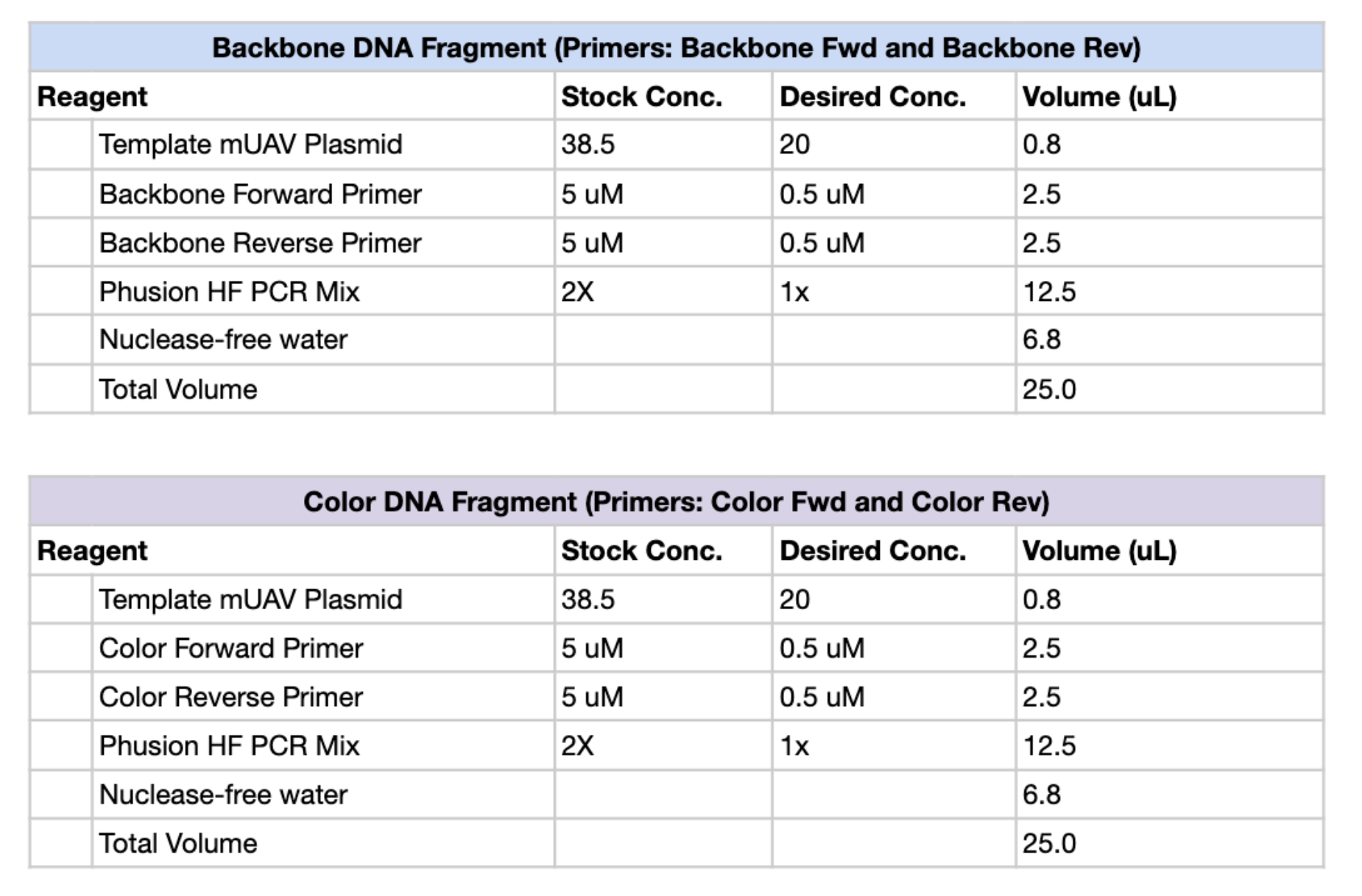
Part 1 1. PCR Figure 1. PCR reaction setup tables for the Backbone DNA Fragment (top) and Color DNA Fragment (bottom), including reagent volumes for a 25 µL total reaction.
Overview In this lab, we designed two neuromorphic genetic circuits using the HTGAA 2026 Genetic Circuit Design Template and simulated their behavior using the Biocompiler-Predict tool. Both circuits are built from endoribonuclease-based sequestrons — the fundamental building blocks of intracellular artificial neural networks (IANNs) — and are intended for transfection into HEK293 cells via Lipofectamine 3000 and execution by an OT-2 liquid handling robot.
Subsections of Labs
Week 1 Lab: Pipetting
Pre-lab answers
Stock MS in g/mL
5 M × 532 g/mol = 2660 g/L = 2.66 g/mL
Serial dilution plan: 5 M → 100 µM
Total dilution = 50,000× → 2 steps.
Step
From → To
Factor
Take stock
+ dH₂O
Final vol
Pipette
1
5 M → 10 mM
500×
2 µL
998 µL
1000 µL
P2/P20 + P1000
2
10 mM → 100 µM
100×
10 µL
990 µL
1000 µL
P20 + P1000
Tubes: 1.5 mL Eppendorfs (volumes too large for PCR strips).
Final reaction (60 µL, MS at 40 µM, dye at 1×)
Reagent
Stock
Final
Volume
Loading dye
6×
1×
10 µL
MS
100 µM
40 µM
24 µL
dH₂O
—
—
26 µL
Total
60 µL
Why 100 µM intermediate instead of diluting straight to 40 µM? 100 µM is a clean serial-dilution endpoint (50,000× = 500× × 100×); 40 µM isn’t. The 100 µM tube also acts as a reusable stock for downstream reactions — error compounds with every extra dilution step, so fewer steps to a clean intermediate is better.
Part 1 — Mixing color (practice)
Followed protocol: tubes 1–3 single colors (500 µL each), tubes 4–6 mixed pairs (R+Y, Y+B, R+B). Two-step pipetting (200 + 20 µL) on tube 4 to practice tip changes.
Plating designs: Used 1–10 µL drops on a glass petri to build volume intuition. Drop diameter scales noticeably with volume — 1 µL drops are barely visible without backlight; 10 µL drops bead high enough to catch reflection.
Result
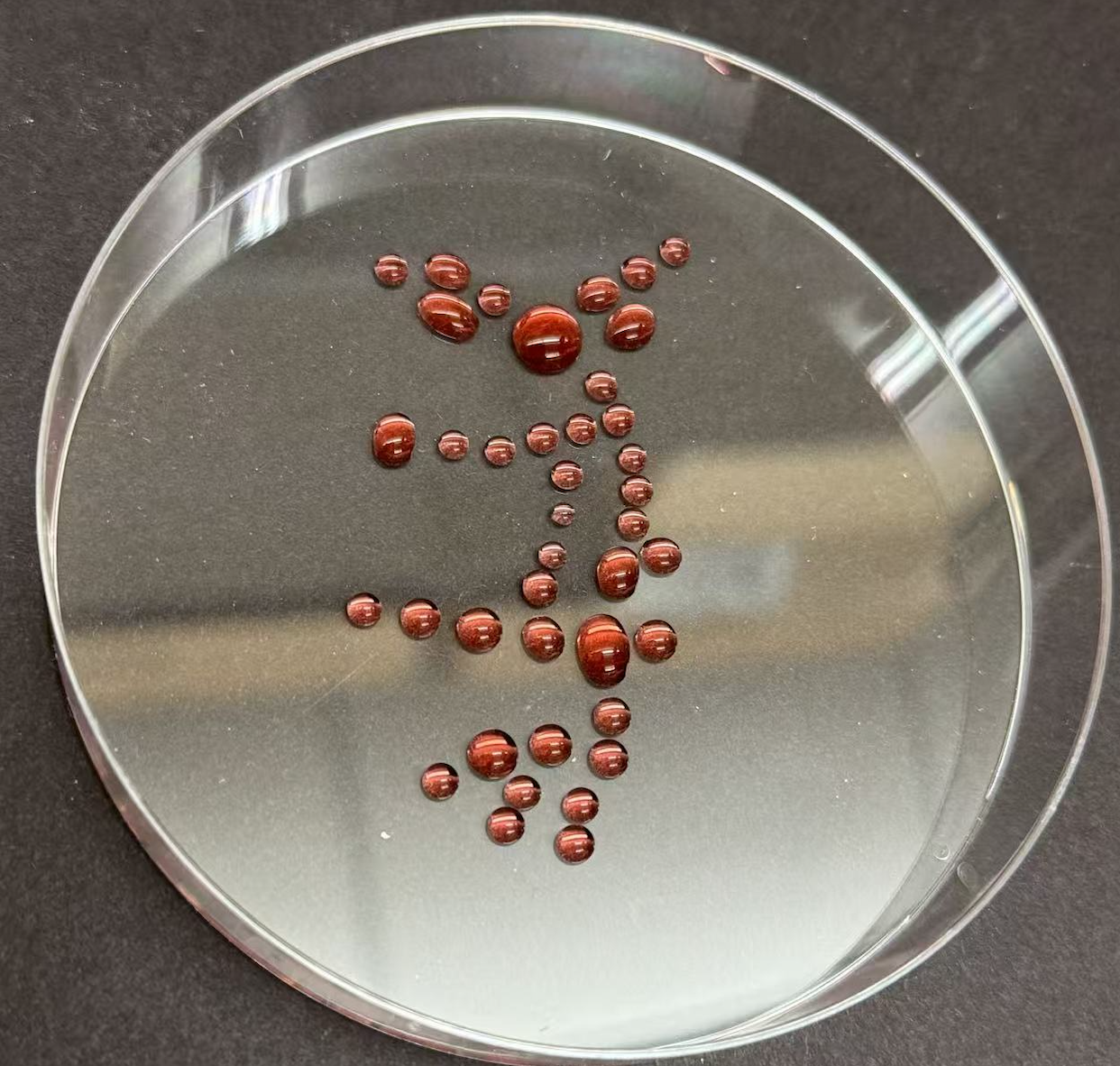
I pipetted the 甲骨文 (oracle bone script) of 马 — the Chinese character for horse — onto the plate to celebrate the Year of the Horse (2026). Oracle bone script is the earliest known form of Chinese writing, carved into ox scapulae and turtle plastrons during the Shang dynasty (~14th–11th c. BCE) for divination. The pictographic form of 马 still shows the horse’s mane, four legs, and tail.
Reference character (甲骨文 of 马)
My pipetted plate
Observations:
Drop size variability across the design = visible record of where my hand was steady vs. shaky.
Surface tension on bare glass keeps drops discrete — no spreading or merging unless they touched.
Part 2 — Serial dilution
Performed the two-step dilution per the table above. Mixed by pipetting up/down 3–4× after each addition. Marked tubes with target concentration.
Prepared the 60 µL final reaction. Loaded 20 µL into a pre-prepared gel well (bonus step) — went in cleanly without puncturing.
Week 11 Lab: Cloud Lab
Part B — Cell-Free Protein Synthesis
B1. Role of each reagent (20 h NMP-Ribose-Glucose mix)
Component
Role in the reaction
BL21 (DE3) Star lysate
Source of ribosomes, tRNAs, aminoacyl-tRNA synthetases, and other translation machinery. (DE3) carries T7 RNAP for transcription; Star = reduced RNase E -> mRNA more stable.
Zwitterionic buffer holds pH near physiological — keeps T7 RNAP and ribosomes active.
Magnesium glutamate
Mg 2+ cofactor for ribosome assembly, T7 RNAP, and aminoacyl-tRNA synthetases. Concentration is highly tunable — too low halts translation, too high promotes misincorporation.
K-phosphate mono/dibasic
Secondary pH buffer + phosphate pool for nucleotide kinase reactions (NMP -> NDP -> NTP).
Ribose
Feeds the salvage pathway: ribokinase -> ribose-5-P -> PRPP, which combines with free bases to form NMPs. Also a slow-burning energy substrate.
Glucose
Carbon source for glycolysis -> continuous ATP regeneration (sustained energy, unlike PEP which burns fast).
AMP / CMP / UMP
NMP precursors. Cellular kinases phosphorylate them to NTPs in situ -> slower ramp than feeding NTPs, but cheaper and less product-inhibition.
GMP (0 mM here)
Omitted in the 20 h mix; GTP is generated via the Guanine salvage path instead (see bonus).
Guanine
Substrate for HGPRT: Guanine + PRPP -> GMP + PPi. Cheaper than buying GMP directly.
17 amino acid mix
Bulk substrate pool for translation (all proteinogenic AAs except Tyr and Cys, which need special handling).
Tyrosine (pH 12)
Added separately — Tyr has very low solubility at neutral pH and must be kept in alkaline solution until dilution.
Cysteine
Added separately — readily oxidizes to cystine (forms disulfides). Kept in its own tube to avoid inactivation before reaction start.
Nicotinamide
NAD+ precursor + inhibitor of NAD-degrading enzymes (NADases) in the lysate -> preserves the redox cofactor pool over the long incubation.
Nuclease-free water
Backfill to final volume; nuclease-free to protect the DNA template and mRNA.
B2. PEP-NTP (1 h) vs NMP-Ribose-Glucose (20 h)
The PEP-NTP mix feeds the reaction with finished NTPs and uses phosphoenolpyruvate as a high-energy ATP regenerator — fast, intense protein synthesis, but PEP is depleted within ~1 hour and the system burns out. The NMP-Ribose-Glucose mix instead supplies precursors (NMPs + ribose for PRPP, glucose for glycolytic ATP) and lets the lysate’s own kinases and salvage enzymes assemble NTPs on demand, giving a slower but sustained ramp that lasts 20+ hours. Cost-per-reaction is also much lower because cheap precursors replace expensive NTPs and PEP.
B3. How can transcription occur without GMP if Guanine is present?
E. coli’s purine salvage pathway rebuilds GMP from free Guanine. Specifically:
So as long as ribose is supplied (to make PRPP) and HGPRT is active in the lysate, free Guanine gets converted to GTP at a rate that supports transcription. This is the same logic the cell uses to recycle purines released from RNA turnover — Ginkgo / OpenAI’s paper exploited it to cut reagent cost.
Part C — Planning the Global Experiment
C1. Biophysical / functional property of each FP that matters for cell-free expression
a. sfGFP (superfolder GFP) — Engineered for robust, fast folding (~13 min maturation) even when fused to aggregation-prone partners. Chromophore (Ser-Tyr-Gly cyclization -> dehydration -> oxidation) requires O2, but maturation is fast enough that O2 rarely limits it in 20 uL wells.
b. mRFP1 — Classic monomeric DsRed-derivative. Slow maturation (~1 h) through a GFP-like green intermediate before red, O2-dependent, and acid-sensitive (pKa ~4.5). Maturation kinetics, not synthesis rate, dominate readout over a 36 h incubation.
c. mKO2 — From Fungia concinna. Acid-stable (pKa ~5.5, lower than most FPs) -> fluorescence is preserved as glycolysis acidifies the well over long incubations. Maturation is fast (~7 min). Bright per molecule.
d. mTurquoise2 — Engineered CFP variant with exceptional quantum yield (~0.93) and long fluorescence lifetime -> very bright per folded molecule. Folding is reliable, but it shares the standard O2 dependence and emits in cyan, requiring the right filter set.
e. mScarlet-I — De novo designed monomeric RFP, “I” = improved maturation (~36 min, vs ~3 h for parent mScarlet). Among the brightest monomeric reds. Acid-sensitive (pKa ~5.4) and O2-dependent — maturation rate is the key bottleneck and matches the 36 h incubation window well.
f. Electra2 — Engineered FP designed for improved photostability / brightness. As with most FPs, chromophore maturation is O2-dependent and folding efficiency at 37 C will set how much of the synthesized protein actually fluoresces; if it’s a slower-folding variant, longer incubation favors it.
C2. Hypothesis
Protein: mScarlet-I (red).
Reagent change: Increase Mg 2+ glutamate from 7 mM to ~10 mM AND extend incubation in mild orbital shaking instead of static.
Expected effect:
Moderately higher Mg 2+ improves T7 RNAP processivity and ribosome activity -> more mScarlet-I polypeptide synthesized within the first 6 h.
Gentle shaking keeps dissolved O2 saturated in the 20 uL droplet, accelerating mScarlet-I’s O2-dependent chromophore oxidation -> more of the synthesized polypeptide reaches the fluorescent state by 36 h.
Net: higher endpoint fluorescence at 36 h vs the control mix.
Risks: Too much Mg 2+ causes misincorporation and aggregation; shaking can foam the lysate. Sweep Mg 2+ in 1 mM increments around 10 mM to find the optimum.
C3. Phase 2 — assigned wells & master mix recipe
Wait for assignment email (by 4/24). Once received, fill in:
Assigned well(s): [e.g., row C col 7, mScarlet-I template]
Custom 2 uL supplement composition (final concentrations after 1:10 dilution into the 20 uL reaction):
[reagent 1: target conc]
[reagent 2: target conc]
[backfill: nuclease-free water]
Reaction recipe per well (20 uL total):
Component
Volume
BL21 (DE3) Star lysate
6 uL
2x Optimized Master Mix
10 uL
Assigned FP DNA template
2 uL
My custom reagent supplement
2 uL
Week 2 Lab: DNA Gel Art
Design (Benchling)
Designed a face: eyes in lanes 1/3/7, eyebrows in lanes 2/6, nose in lane 5, lips in lane 4.
Digest setup (per lane, 20 µL total)
Lane
Enzyme(s)
Water
CutSmart 10×
λ DNA (0.5 µg/µL)
Enzyme(s) (1 µL each)
1
PvuII + SalI
13 µL
2 µL
3 µL
1 + 1 µL
2
BamHI + XhoI
13 µL
2 µL
3 µL
1 + 1 µL
3
PvuII + SalI
13 µL
2 µL
3 µL
1 + 1 µL
4
SalI only
14 µL
2 µL
3 µL
1 µL
5
NdeI + PvuII
13 µL
2 µL
3 µL
1 + 1 µL
6
BamHI + XhoI
13 µL
2 µL
3 µL
1 + 1 µL
7
PvuII + SalI
13 µL
2 µL
3 µL
1 + 1 µL
Incubated at 37 °C, 30 min.
Predicted gel (Benchling virtual digest, NEB 2-Log ladder)
Bench setup
Enzymes, λ DNA, 6× loading dye, and rCutSmart buffer kept on ice. Visible on ice: λ DNA, SacI, KpnI (×2), BamHI, FD PvuII (FastDigest), rCutSmart, Eco32I (= EcoRV), 6× LD.
Gel prep & run
1% agarose: 0.75 g agarose in 75 mL 1× TAE → microwave in 15 s pulses → cool to ~50 °C → 7.5 µL SYBR Safe (10,000×) → pour with 12-well comb → set 30 min.
Gel did not match the predicted pattern. Bands were either absent, smeared, or in unexpected positions. The face design was not recoverable.
Failure analysis — most likely causes
Buffer × enzyme mismatch (top suspect). Ice bucket shows FD PvuII (Thermo FastDigest) but digests used rCutSmart (NEB). FastDigest enzymes are optimized for Thermo’s FastDigest buffer; activity in CutSmart is partial. PvuII appears in 4 of 7 lanes (1, 3, 5, 7) — one mismatch collapses most of the design.
NdeI / XhoI not confirmed on the bench. Neither tube visible on ice. If a substitute was grabbed, lanes 2, 5, 6 wouldn’t cut as designed.
Run voltage / time. Smearing and blended rows = classic too-fast / too-long signature. 115 V is on the high end; try 70–90 V.
DNA overload. 1.5 µg per digest × 20 µL loaded ≈ 150 ng/well, over the 100 ng/well guideline.
Incomplete digestion. 30 min is the floor; 60 min helps with non-optimal buffers.
Next time — checklist
Cross-check enzyme list on the bench before finalizing the Benchling design.
If using FastDigest enzymes, use FastDigest buffer, not CutSmart. Don’t mix systems.
NEB Double Digest Finder for any 2-enzyme combo.
Nanodrop the λ DNA; dilute so each lane loads ≤ 100 ng.
Run at 80–90 V for 45–60 min; stop when dye front is ~⅔ down.
Photograph the gel with the ladder lane clearly visible.
Week 3 Lab: Opentrons Art
Week 6 Lab: Gibson Assemly
Week 6: Gibson Assembly
Group members: Louisa Zhu, Shitong, Jasmin
Part 1
1. PCR
Figure 1. PCR reaction setup tables for the Backbone DNA Fragment (top) and Color DNA Fragment (bottom), including reagent volumes for a 25 µL total reaction.
We then ran the PCR reaction with the following thermocycler settings:
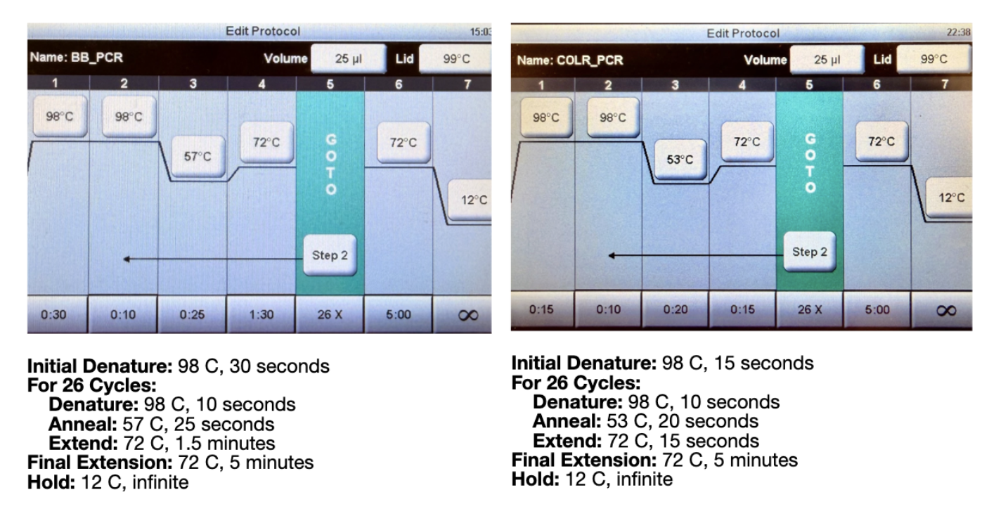
Figure 2. Thermocycler programs for the backbone PCR (BB_PCR, left) and color fragment PCR (COLR_PCR, right). Both protocols use 26 cycles with a final extension at 72°C for 5 minutes.
2. Gel Eletrophoresis
Protocol credit to Louisa:
Take 2 µL of each mixture and transfer into new labeled PCR tubes
Pipette 2 µL of mUAV into a new tube
Add 20 µL of water to each PCR tube
Unpack gel electrophoresis cassette and load into machine
Pipette DNA Ladder into first well
Pipette 20 µL of mixture from each new PCR tube into correct wells (6 full wells total)
Use the automatic setting for 1%, wait 10 minutes
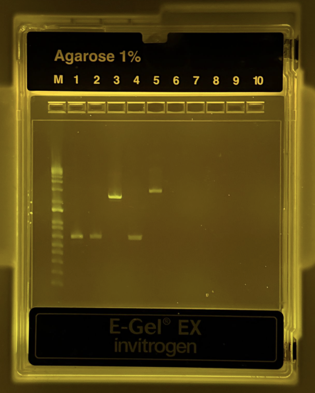
Figure 3. Agarose 1% gel electrophoresis result showing PCR products. The DNA ladder (M) is in the first lane. Bands are visible for the backbone and color fragments, confirming successful amplification.
After PCR amplification, a 1% agarose gel electrophoresis was performed to verify the size and quality of the amplified fragments. As shown in Figure 3, distinct bands were observed in the expected lanes, with the backbone fragment appearing at approximately 1.5 kb and the color fragments (Light Pink, Blue, and Purple) resolving at approximately 500–800 bp. All bands were sharp and well-defined with no visible smearing or non-specific secondary bands, indicating high-specificity amplification with minimal off-target products. The absence of bands in the negative control lane further confirms that there was no contamination during the PCR setup. The fragment sizes observed are consistent with the expected sizes based on the primer design and template mUAV plasmid, confirming that the correct regions were successfully amplified. These results demonstrate that both the backbone and color fragment PCR reactions performed as expected, and that the purified products were of sufficient quality to proceed to Gibson Assembly.
3. DNA Purification and Quantification
Pipette 100 µL of DNA Binding Buffer into a centrifuge tube
Add 20 µL of PCR product
Mix briefly by vortexing
Transfer 120 µL of the mixture into separate columns with a collection tube
Centrifuge for 1 minute
Discard the flowthrough
Add 200 µL of DNA wash buffer to the column
Centrifuge for 1 minute
Repeat the last two steps
Transfer the column to a new tube
Discard flowthrough
Add 6 µL of nuclease-free water to the column matrix
Allow to sit for 2 minutes
Centrifuge for 1 minute
Store and save
Part Two
Materials (Credit to Lousia)
Items used:
P1000 pipette with 1000 µL tips
P20 pipette with 10 µL tips
PCR Tubes
Biological materials:
Purified Fragments
Gibson Assembly Master Mix
Nuclease-Free Water
LB-Agar plates with Chloramphenicol
SOC Growth Medium
DH5α competent cells
Machines used:
Thermal Cycler
Shaking Incubator
Waterbath set to 42°C
Part 1: Setting Up Gibson Assembly
We set up reactions in the proportions shown below for each color fragment, then incubated at 50°C for 30 minutes in a heat block, followed by adding 100 µL of nuclease-free water to dilute each sample.
Reagent
Stock Conc. (ng/µL)
Desired Conc. (ng/µL)
Volume (µL)
Backbone Fragment
50
25
0.5
Color Fragment (Single)
50
50
1.0
Gibson Assembly Mix
2X
1X
5
Nuclease-free water
—
—
3.5
Total Volume
10
Part 2: Transformation
Transfer 20 µL of competent cells to each tube
Transfer purified assembly products into each tube (8 total: 3 Light Pink, 3 Blue, 3 Purple)
Incubate on ice for 30 minutes
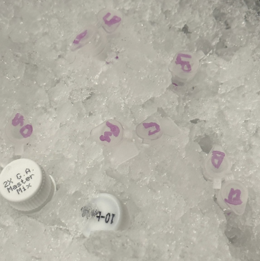
Figure 4. Tubes incubating on ice during the transformation step. Each tube is labeled by color and sample number.
Heat shock the cells at 42°C for 45 seconds immediately after the ice bath
Add 100 µL of SOC media to each tube
Allow growth in a shaking incubator for 1 hour
Transfer 100 µL from each tube to the appropriate plate and spread using plating beads or a plastic spreader
Incubate plates at 37°C for 72 hours
Part 3. Results
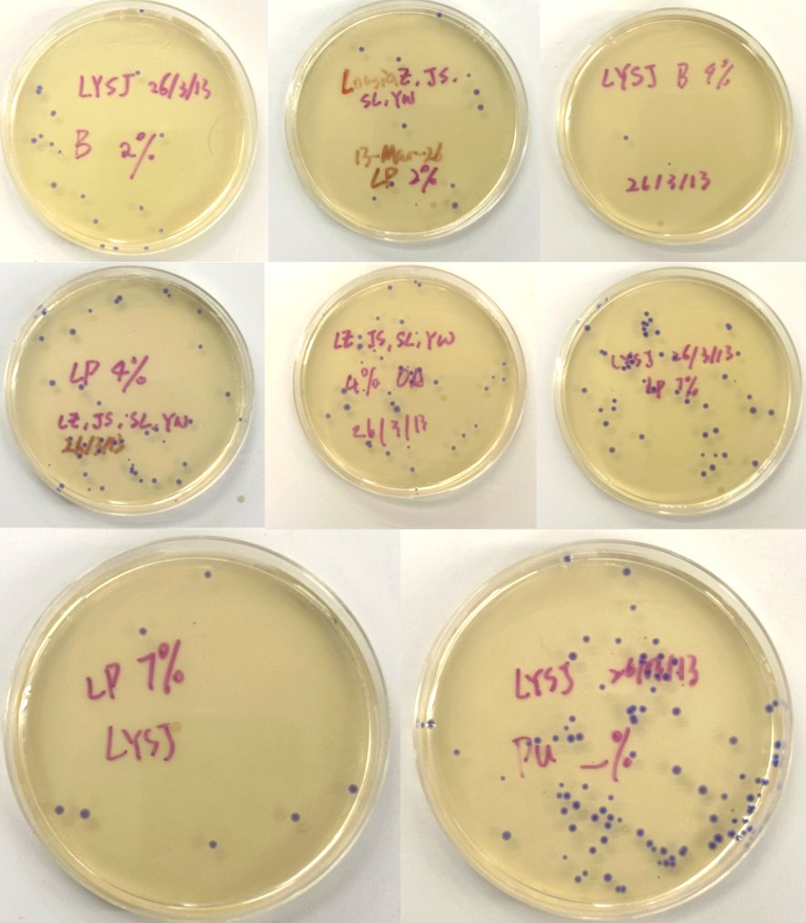
Figure 5 (A-H). LB-Agar plates with Chloramphenicol selection showing colony growth after transformation. Plates were labeled by color fragment condition Blue (B), Light Pink (LP), and Purple (Pu) at varying dilutions (Subject to correction with further observation). Interestingly, all colonies grew out purple-blue regardless of which color fragment was used. This may be because the insert DNA was not incorporated at the right ratio relative to the backbone, causing cells to express the backbone’s default color instead.
Week 7 Lab: Neuromorphic Circuits
Overview
In this lab, we designed two neuromorphic genetic circuits using the HTGAA 2026 Genetic Circuit Design Template and simulated their behavior using the Biocompiler-Predict tool. Both circuits are built from endoribonuclease-based sequestrons — the fundamental building blocks of intracellular artificial neural networks (IANNs) — and are intended for transfection into HEK293 cells via Lipofectamine 3000 and execution by an OT-2 liquid handling robot.
Key components used:
Csy4 — a CRISPR endoribonuclease that cleaves mRNA at its recognition sequence
CasE (EcoCas6e) — a second orthogonal endoribonuclease for independent mRNA cleavage
PgU — a constitutive expression construct
mNeonGreen, mKO2, eBFP2 — fluorescent protein reporters (green, orange, blue)
_rec_ notation indicates a recognition site (e.g., Csy4_rec_mNeonGreen = mNeonGreen mRNA with a Csy4 cleavage site)
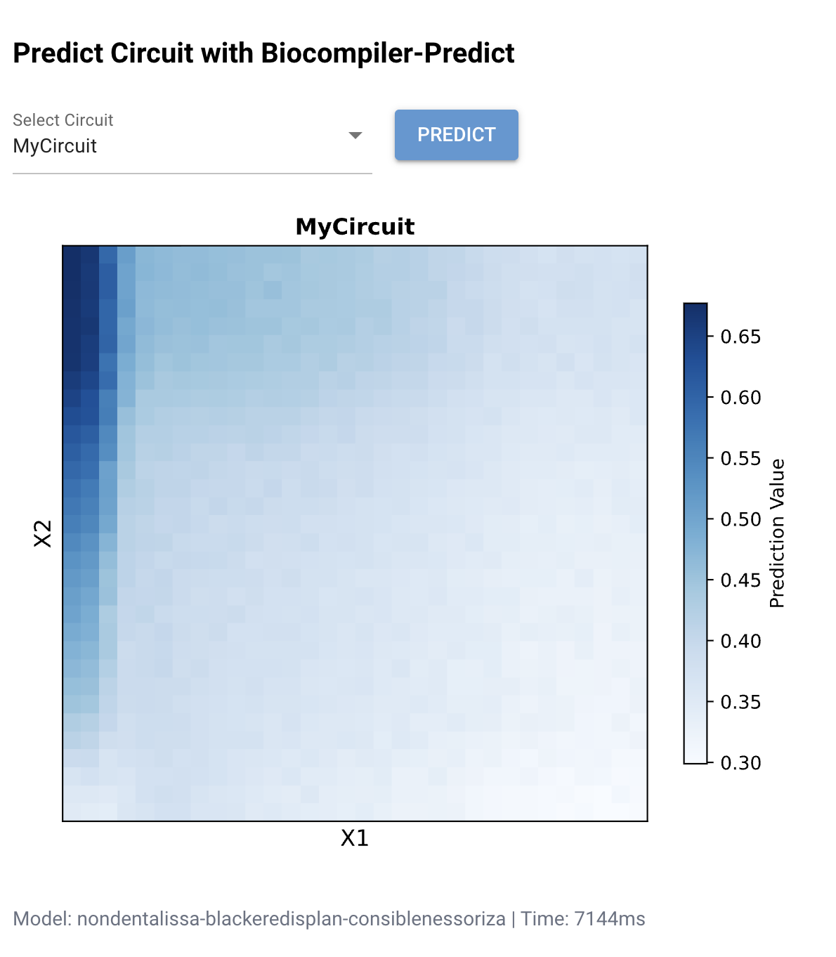
Circuit 1: “MyCircuit” (L-shape response)
Design rationale
This circuit implements a single-layer perceptron where two inputs (X₁ and X₂) each produce an endoribonuclease that negatively regulates a shared fluorescent output. The goal was to achieve an L-shaped dose–response surface: the output (mNeonGreen) should be high only when both inputs are low.
Analogy: Think of it like two faucets draining a bathtub. If either faucet is open (high X₁ or high X₂), water drains out and the tub level drops. The tub is full only when both faucets are closed.
Circuit design table
Circuit name
Transfection group
Contents
Concentration (ng/µL)
DNA wanted (ng)
MyCircuit
X1
Csy4
40
150
MyCircuit
X1
mKO2
50
100
MyCircuit
X2
CasE
50
150
MyCircuit
X2
eBFP2
50
100
MyCircuit
bias_output_csy4
Csy4_rec_mNeonGreen
50
100
MyCircuit
bias_output_case
CasE_rec_mNeonGreen
50
100
Total DNA: 700 ng
How it works
X₁ input delivers Csy4 endoribonuclease DNA (150 ng) along with mKO2 (orange fluorescent protein, 100 ng) as a transfection marker to verify X₁ delivery.
X₂ input delivers CasE endoribonuclease DNA (150 ng) along with eBFP2 (blue fluorescent protein, 100 ng) as a transfection marker for X₂.
Output layer consists of mNeonGreen mRNA with recognition sites for both Csy4 (Csy4_rec_mNeonGreen, 100 ng) and CasE (CasE_rec_mNeonGreen, 100 ng). Both endoribonucleases independently cleave the output mRNA.
When X₁ is high → more Csy4 is produced → more mNeonGreen mRNA is cleaved → output decreases.
When X₂ is high → more CasE is produced → more mNeonGreen mRNA is cleaved → output decreases.
When both are low → minimal cleavage → mNeonGreen output is maximal.
Predicted behavior
Figure 1: Biocompiler-Predict simulation of MyCircuit. The heatmap shows the predicted mNeonGreen output (Prediction Value) as a function of X₁ and X₂ concentrations. High output (dark blue, ~0.65–0.70) is concentrated along the left edge where X₁ is low. The L-shaped pattern confirms that the circuit acts as an approximate NOR-like function: output is highest when inputs are minimal.
Interpretation
The simulation reveals that X₁ (Csy4) has a stronger suppressive effect on the output than X₂ (CasE), as evidenced by the sharp drop-off along the X₁ axis compared to a more gradual decline along X₂. This asymmetry likely reflects differences in the catalytic efficiency and binding affinity of Csy4 versus CasE for their respective recognition sequences on the mNeonGreen mRNA. The L-shaped pattern is consistent with a weighted NOR gate where the X₁ weight is larger than the X₂ weight.
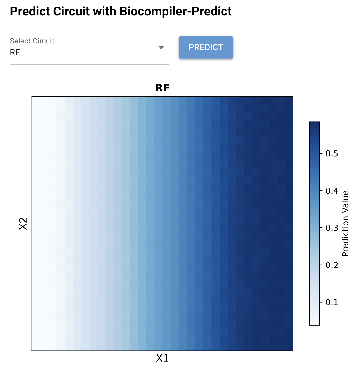
Circuit 2: “RF” (Rectified function)
Design rationale
This circuit implements a more complex multilayer architecture with cross-regulation between endoribonucleases. The goal was to achieve a rectified function — an output that increases monotonically with X₁ while remaining relatively insensitive to X₂, similar to a ReLU (rectified linear unit) activation function in machine learning.
Analogy: Imagine a volume knob (X₁) that smoothly turns up the music, while a second knob (X₂) has little effect because its signal gets cancelled out by internal feedback. The circuit “learns” to listen to one input and ignore the other.
Circuit design table
Circuit name
Transfection group
Contents
Concentration (ng/µL)
DNA wanted (ng)
RF
X1
CasE
50
100
RF
X2
Csy4
50
100
RF
Bias
PgU
50
100
RF
Bias
CasE_rec_Csy4
50
75
RF
Bias
Csy4_rec_CasE
50
75
RF
Bias
PgU_rec_CasE
50
75
RF
Bias
PgU_rec_Csy4
50
75
RF
X1
CasE_rec_Csy4_rec_mKO2
50
50
RF
X2
Csy4_rec_mNeonGreen
50
50
Total DNA: 700 ng
How it works
This is a multilayer circuit with cross-inhibition between the two endoribonucleases:
X₁ input delivers CasE (100 ng) and a reporter CasE_rec_Csy4_rec_mKO2 (50 ng) — an mKO2 mRNA that can be cleaved by both CasE and Csy4, acting as a dual-regulated node.
X₂ input delivers Csy4 (100 ng) and Csy4_rec_mNeonGreen (50 ng) — mNeonGreen output that is negatively regulated by Csy4.
Bias layer creates a rich cross-regulatory network:
PgU (100 ng) — constitutive expression baseline
CasE_rec_Csy4 (75 ng) — Csy4 mRNA with a CasE recognition site (CasE cleaves Csy4 mRNA)
Csy4_rec_CasE (75 ng) — CasE mRNA with a Csy4 recognition site (Csy4 cleaves CasE mRNA)
PgU_rec_CasE (75 ng) — constitutive mRNA regulated by CasE
PgU_rec_Csy4 (75 ng) — constitutive mRNA regulated by Csy4
The cross-inhibition (CasE_rec_Csy4 and Csy4_rec_CasE) creates a mutual negative feedback loop between the two endoribonucleases. This effectively implements a winner-take-all competition: when X₁ drives CasE production, CasE degrades Csy4 mRNA, further reducing Csy4 levels and amplifying the X₁ signal. The result is a rectified response that primarily follows X₁.
Predicted behavior
Figure 2: Biocompiler-Predict simulation of the RF circuit. The heatmap shows a smooth left-to-right gradient where output increases monotonically with X₁ (left axis = low, right axis = high). The output ranges from ~0.05 (white, low X₁) to ~0.55 (dark blue, high X₁). The response is largely independent of X₂, confirming the rectified function behavior.
Interpretation
The RF circuit successfully achieves a unidirectional dose–response: output scales with X₁ concentration while remaining approximately flat across X₂ values. This behavior arises from the mutual antagonism between Csy4 and CasE in the bias layer. When X₁ increases CasE levels, CasE degrades the Csy4_rec_CasE mRNA (reducing Csy4 production), which in turn reduces degradation of CasE mRNA — a positive feedback amplification of the X₁ signal. Meanwhile, X₂-driven Csy4 is counteracted by CasE from both the X₁ input and the bias layer, preventing X₂ from significantly influencing the output.
The smooth gradient (rather than a sharp threshold) reflects the analog nature of the IANN — the circuit computes a continuous function rather than a binary switch.
Comparison of the two circuits
Feature
MyCircuit (L-shape)
RF (Rectified function)
Architecture
Single-layer, two independent inhibitors
Multilayer with cross-inhibition
Number of parts
6
9
Total DNA
700 ng
700 ng
Output reporter
mNeonGreen
mKO2 / mNeonGreen
Input-output behavior
NOR-like: high when both inputs low
ReLU-like: scales with X₁, ignores X₂
Key design feature
Independent cleavage of shared output
Mutual antagonism creates winner-take-all
Predicted dynamic range
~0.30 – 0.70
~0.05 – 0.55
Methods
Circuit design (Day 1)
Circuits were designed using the HTGAA 2026 Genetic Circuit Design Template (Google Sheet).
Part names followed the conventions in the HTGAA 2026 Genetic Circuit Part Names list.
All concentrations were set to 50 ng/µL (with one exception: Csy4 in MyCircuit at 40 ng/µL).
Circuit behavior was simulated using the Biocompiler-Predict tool, which generates heatmaps of predicted output across the X₁–X₂ input space.
Completed spreadsheets were uploaded via the Google Form submission.
Transfection and imaging (Day 2)
HEK293 cells were transfected using Lipofectamine 3000 with the designed plasmid mixes.
An OT-2 liquid handling robot in the Weiss Lab (NE-47, MIT campus) executed the transfection protocol based on our uploaded spreadsheet.
Fluorescence readout of mNeonGreen, mKO2, and eBFP2 will be measured after 24–48 hours of incubation.
Key takeaways
Analog beats digital: Both circuits produce continuous, graded outputs rather than binary on/off responses — demonstrating the fundamental advantage of IANNs over traditional Boolean genetic circuits.
Weight tuning via DNA dosage: The behavior of each circuit was tuned entirely by adjusting the nanogram amounts of each plasmid. No new genetic parts were needed — only different ratios of the same library components.
Cross-inhibition enables complex functions: The RF circuit shows that mutual antagonism between endoribonucleases can create winner-take-all dynamics, allowing one input to dominate. This is a biological implementation of competitive inhibition analogous to lateral inhibition in neural circuits.
Simulation before wet lab: The Biocompiler-Predict tool allowed us to iterate on circuit designs computationally before committing to expensive and time-consuming wet lab experiments.