Week 3 HW: Lab Automation

Assignment: Python Script for Opentrons Artwork

Artistic Concept — “ELM Habitat Cross-Section”

My design uses the 96-well plate as a canvas to depict a cross-sectional schematic of the Multi-Trophic Myco-Foundry — the engineered living material (ELM) habitat I proposed in Week 1. Three food-safe dyes, pipetted by the Opentrons OT-2, fill concentric rings of wells representing the three biological layers of the habitat:

Ring	Wells	Dye	Biological Layer
Outer (radius 3.0–5.0)	40 wells	Coomassie Blue	Structural Shell — fungal mycelium providing radiation shielding
Middle (radius 1.5–3.0)	28 wells	Sunset Yellow	Vascular System — bacterial network transporting phosphite and metabolites
Core (radius < 1.5)	4 wells	Brilliant Green	Metabolic Hub — B. subtilis pharmaceutical production layer

Wells are classified by Euclidean distance from the geometric center of the plate (between wells D6, D7, E6, E7). The result is a visually clean concentric-ring pattern that mirrors the habitat’s layered architecture.

Plate Layout

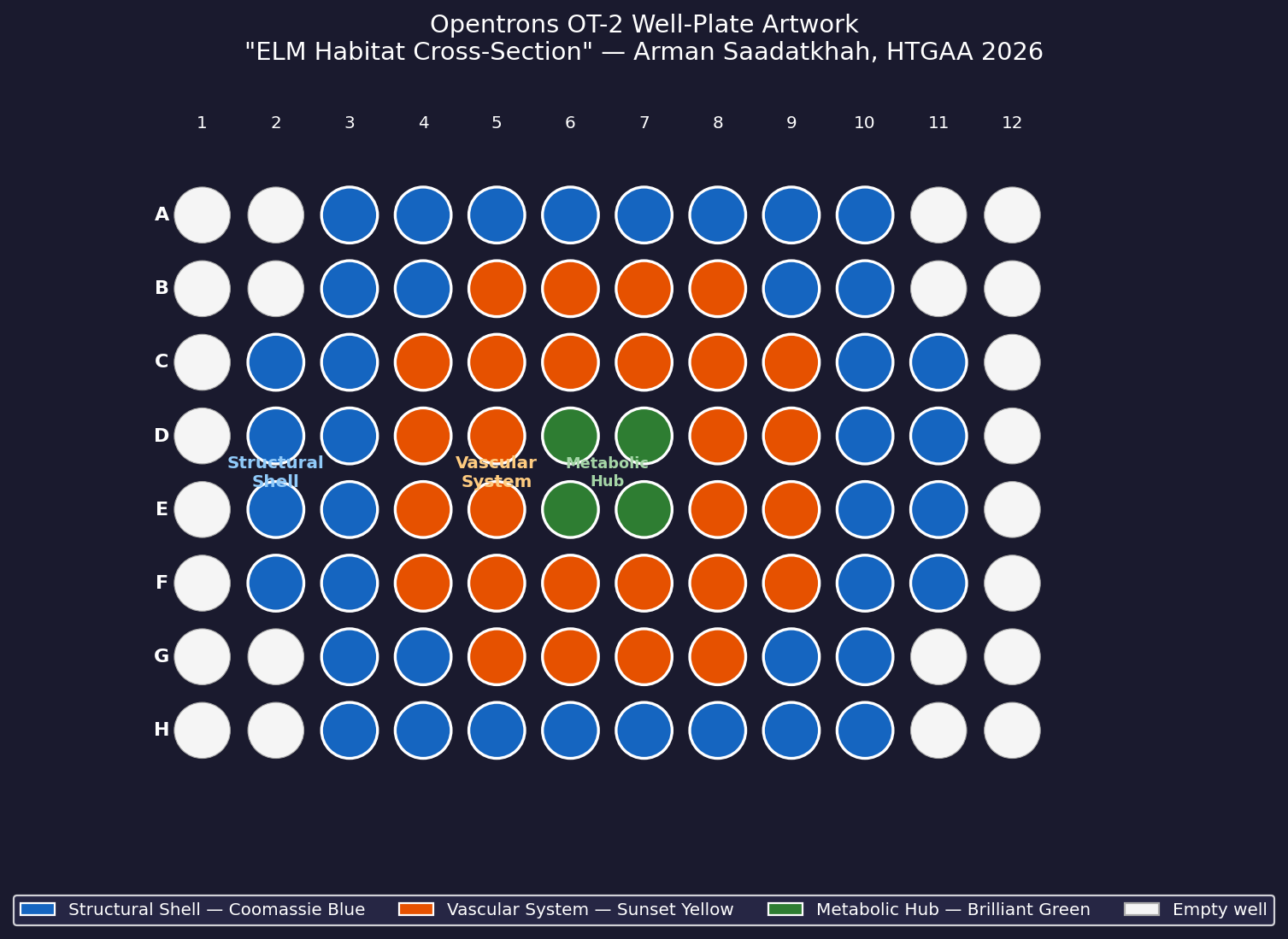Fig 1. Well-plate layout for “ELM Habitat Cross-Section.” Blue = Structural Shell (40 wells), Orange = Vascular System (28 wells), Green = Metabolic Hub (4 wells). Empty wells (corners and edges beyond radius 5.0) are left unfilled.

Python Script (Opentrons API v2.14)

The full protocol is in elm_habitat_opentrons.py. Key design decisions:

new_tip='always' — a fresh tip is used for every well to prevent dye cross-contamination between layers
blow_out=True — residual dye is expelled back into the source well after each transfer, minimising carry-over
VOLUME_UL = 60 µL — sufficient volume for visible colour saturation in a standard flat-bottom 360 µL plate
Wells are computed programmatically via distance formula rather than hand-entered coordinates, making the design easy to rescale or modify

from opentrons import protocol_api
import math

metadata = {
    'protocolName': 'ELM Habitat Cross-Section — Opentrons Art',
    'author': 'Arman Saadatkhah <saadatarman@gmail.com>',
    'apiLevel': '2.14',
}

ROWS = list('ABCDEFGH')
COLS = list(range(1, 13))
ROW_CENTER, COL_CENTER = 3.5, 5.5
VOLUME_UL = 60

def classify_well(ri, ci):
    d = math.sqrt((ri - ROW_CENTER)**2 + (ci - COL_CENTER)**2)
    if d < 1.5:             return 'hub'
    elif 1.5 <= d < 3.0:   return 'vascular'
    elif 3.0 <= d <= 5.0:  return 'shell'
    return 'empty'

def run(protocol: protocol_api.ProtocolContext):
    tiprack_1 = protocol.load_labware('opentrons_96_tiprack_300ul', 1)
    tiprack_2 = protocol.load_labware('opentrons_96_tiprack_300ul', 4)
    plate     = protocol.load_labware('corning_96_wellplate_360ul_flat', 2)
    reservoir = protocol.load_labware('usascientific_12_reservoir_22ml', 3)
    p300 = protocol.load_instrument('p300_single_gen2', 'left',
                                    tip_racks=[tiprack_1, tiprack_2])

    blue   = reservoir['A1']  # Structural Shell
    orange = reservoir['A2']  # Vascular System
    green  = reservoir['A3']  # Metabolic Hub

    shell_wells, vascular_wells, hub_wells = [], [], []
    for ri, row in enumerate(ROWS):
        for ci, col in enumerate(COLS):
            kind = classify_well(ri, ci)
            wn = f"{row}{col}"
            if kind == 'shell':    shell_wells.append(plate[wn])
            elif kind == 'vascular': vascular_wells.append(plate[wn])
            elif kind == 'hub':    hub_wells.append(plate[wn])

    p300.transfer(VOLUME_UL, blue,   shell_wells,
                  new_tip='always', blow_out=True, blowout_location='source well')
    p300.transfer(VOLUME_UL, orange, vascular_wells,
                  new_tip='always', blow_out=True, blowout_location='source well')
    p300.transfer(VOLUME_UL, green,  hub_wells,
                  new_tip='always', blow_out=True, blowout_location='source well')

Reagent volumes required:

Reservoir A1 (blue): ≥ 3.0 mL (40 wells × 60 µL + dead volume)
Reservoir A2 (orange): ≥ 2.0 mL (28 wells × 60 µL + dead volume)
Reservoir A3 (green): ≥ 0.5 mL (4 wells × 60 µL + dead volume)

Estimated run time: ~25 minutes (72 tip changes × ~20 s/transfer)

AI Disclosure

Claude Sonnet 4.6 (Anthropic) was used to assist with script structure, geometric well-classification logic, and blowout/tip-change parameter selection. The artistic concept (ELM habitat cross-section), biological layer assignments, and dye colour choices were developed by the student.

Post-Lab Questions

Q1 — Published Paper Using Opentrons for Novel Biological Applications

Brown DM, Phillips DA, Garcia DC, Karim AS, Jewett MC, Styczynski MP, et al. “Semiautomated Production of Cell-Free Biosensors.” ACS Synthetic Biology, 2025, 14(3): 979–986. DOI: 10.1021/acssynbio.4c00703

What they automated and why it was novel:

The authors used the Opentrons OT-2 to semiautomatically assemble and screen cell-free protein synthesis (CFPS) biosensor reactions in a 96-well format. Each reaction contained a genetically encoded biosensor — a transcription factor coupled to a fluorescent reporter — that signals the presence of a specific analyte (heavy metals, metabolites, or toxins) in a sample.

Previously, CFPS biosensor production required tedious manual pipetting of 8–12 components per reaction, making high-throughput screening impractical. The Opentrons OT-2 automated the liquid handling — dispensing cell lysate, DNA templates, buffer components, and analyte samples — reducing hands-on time from hours to minutes and enabling the team to test dozens of biosensor variants and analyte concentrations in a single run.

Why it matters for HTGAA: This paper demonstrates a direct path from the “design a protein” step (Week 4) to “deploy it as a sensor” step using lab automation. For my ELM habitat project, the same pipeline could be used to screen the CFPS-based pharmaceutical payload — synthesizing and testing different drug-producing constructs automatically before committing them to the living material system.

Q2 — Automation Plan for the ELM Habitat Final Project

Goal: Use lab automation to screen and validate the phosphite auxotrophy biocontainment system — verifying that ptxD-expressing bacteria survive in phosphite-supplemented media and die in phosphate-only media, across a range of concentrations.

Overview

The Opentrons OT-2 will run a 12-condition × 8-replicate growth screen on a standard 96-well plate, testing the ptxD-based kill switch across a 2-fold phosphite dilution series alongside a phosphate-only control. A fluorescent reporter (GFP driven by a growth-responsive promoter) provides a real-time readout of bacterial viability.

Automation Workflow

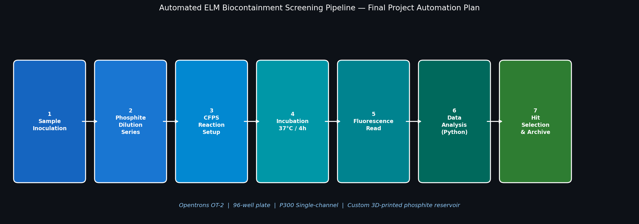Fig 2. Seven-step Opentrons automation pipeline for screening the ELM phosphite auxotrophy kill switch. Steps 1–5 are executed by the OT-2; Steps 6–7 use downstream software analysis.

Step	Action	Opentrons Role
1	Inoculate 96-well plate with ptxD-expressing B. subtilis	P300 multi-channel transfer from overnight culture
2	Dispense phosphite dilution series (columns 1–10) + phosphate control (cols 11–12)	P300 serial dilution across plate columns
3	Add CFPS master mix to designated sensor wells	P20 single-channel for precision low-volume addition
4	Seal plate, transfer to incubator (37°C, 4 h)	OT-2 deck module (Opentrons Heater-Shaker)
5	Transfer 20 µL from each well to black assay plate	P20 multi-channel transfer
6	PHERAstar plate reader: GFP fluorescence at Ex 485 / Em 520 nm	Offline (reader not on OT-2 deck)
7	Python analysis: fit Hill equation to phosphite–viability curve, compute IC₅₀	Automated data pipeline

Pseudocode

# Step 2: Phosphite serial dilution (2-fold, columns 1-10)
phosphite_stock = reservoir['A1']   # 100 mM phosphite
media_blank     = reservoir['A2']   # phosphate-free M9 minimal media

# Seed col 1 with 100 mM phosphite
p300.transfer(100, phosphite_stock, plate.columns()[0])

# Serial 2-fold dilution across columns 1 → 10
for col_idx in range(9):
    p300.transfer(100,
                  plate.columns()[col_idx],
                  plate.columns()[col_idx + 1],
                  mix_after=(3, 80),
                  new_tip='always')

# Columns 11-12: phosphate-only negative control
phosphate_ctrl = reservoir['A3']    # 5 mM phosphate (no phosphite)
p300.transfer(100, phosphate_ctrl, plate.columns()[10:12])

# Step 3: Add bacteria + GFP reporter
bacteria = reservoir['A4']
p300.transfer(50, bacteria, plate.wells(), new_tip='always')

3D-Printed Accessories

A custom 3D-printed phosphite reservoir adapter will be designed using the Opentrons 3D Printing Directory to hold four 15 mL falcon tubes at the correct deck height for the P300. This allows the phosphite stock to be swapped without reconfiguring the deck layout between runs.

Connection to Final Project

This screen directly validates the synthetic auxotrophy layer of the ELM habitat. A well-characterized phosphite IC₅₀ value is required before the ptxD-modified organisms can be deployed in a simulated Mars regolith environment — providing the quantitative biocontainment threshold needed for the safety case to COSPAR. Automating this screen with Opentrons allows 96-condition testing in a single afternoon rather than the 2–3 days required for manual plate setup.

Disclaimer: AI (Claude Sonnet 4.6) was used to assist with pseudocode formatting and automation workflow design. The biological rationale, experimental design, and project connection were developed by the student.