Week 1 Lab: Introduction to Pipetting and Dilutions

Overview

This first HTGAA lab introduces the foundational techniques of pipetting and serial dilutions — critical skills for precise liquid handling in biological and chemical experiments. Two protocols were covered: mixing food coloring solutions to build volume intuition, and performing a serial dilution of a mystery substance (MS) to achieve a target concentration.

Pre-Lab

Key Definitions

Dilution Formula

The core equation for all dilution calculations:

C₁V₁ = C₂V₂

Rearranged to find the transfer volume: V₁ = (C₂ × V₂) / C₁

Volume of water to add: V_water = V₂ − V₁

Dilution Practice 1

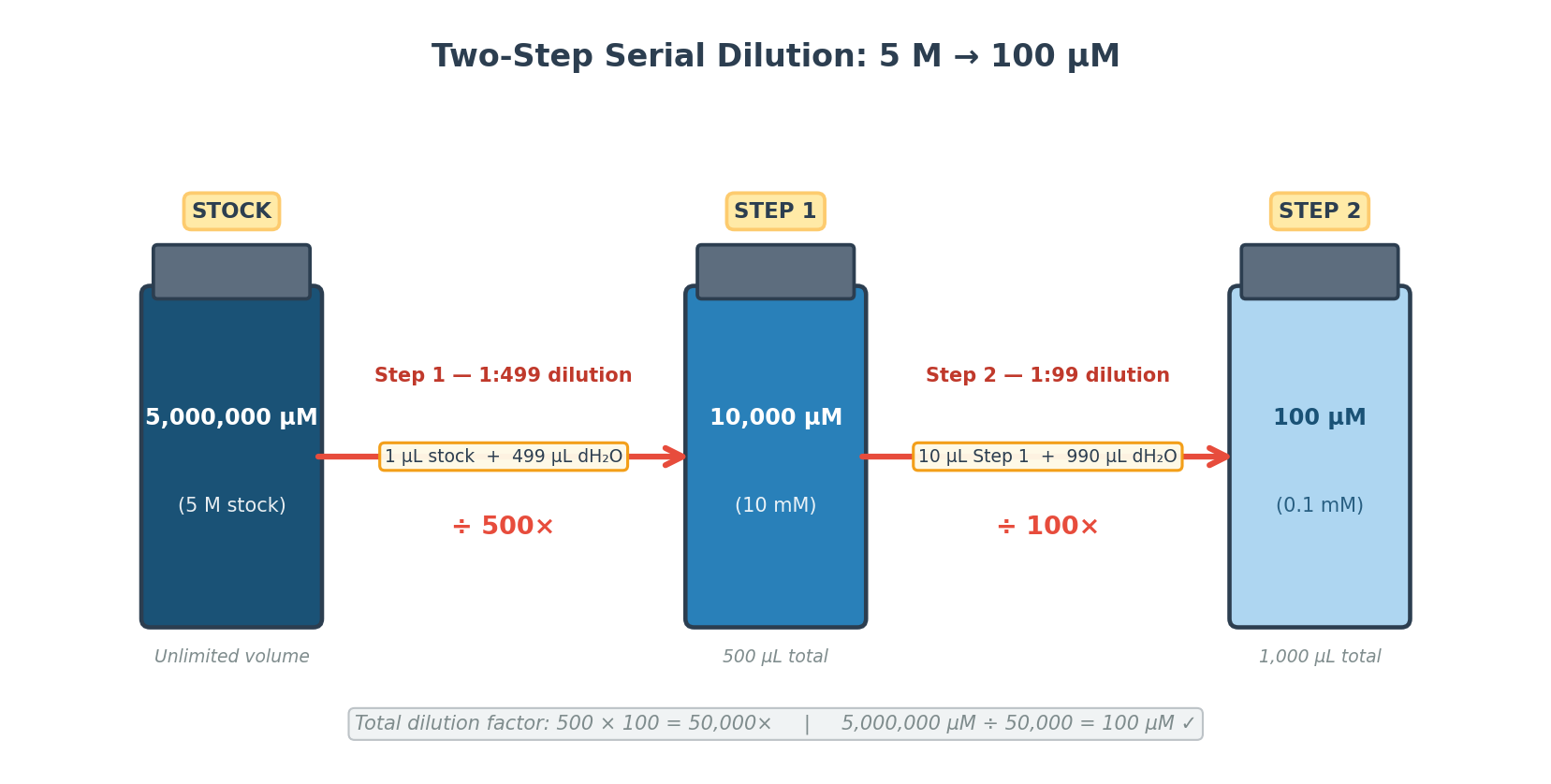
Scenario: Stock [MS] = 5 M. Goal: reach 100 µM using two sequential steps.

Step 1 — 5 M → 10,000 µM (1:499 dilution, 500× dilution factor)

Using C₁V₁ = C₂V₂ with V₂ = 500 µL:

V₁ = (10,000 µM × 500 µL) / 5,000,000 µM = 1 µL of 5 M stock

V_water = 500 − 1 = 499 µL of dH₂O

Result: 500 µL at 10,000 µM (10 mM)

Step 2 — 10,000 µM → 100 µM (1:99 dilution, 100× dilution factor)

Using C₁V₁ = C₂V₂ with V₂ = 1000 µL:

V₁ = (100 µM × 1000 µL) / 10,000 µM = 10 µL of Step 1 solution

V_water = 1000 − 10 = 990 µL of dH₂O

Result: 1000 µL at 100 µM — total dilution factor = 500 × 100 = 50,000×

Dilution Practice 2

Part a — Stock concentration in g/mL

Given: stock = 5 M, molar mass = 532 g/mol

5 mol/L × 532 g/mol = 2,660 g/L = 2.66 g/mL

Part b — Serial dilution plan from 5 M to 100 µM

Total required dilution factor: 5,000,000 µM ÷ 100 µM = 50,000×

A single dilution step is impractical — transferring 1 µL into 50 mL introduces unacceptable pipetting error at the microliter scale. A two-step serial dilution distributes the dilution factor into two manageable operations:

Two dilution steps total. Eppendorf tubes are used at each step because they hold up to 1.5 mL and snap closed securely. The P20 pipette handles small transfers (1–10 µL) with precision; the P1000 adds the bulk water volumes.

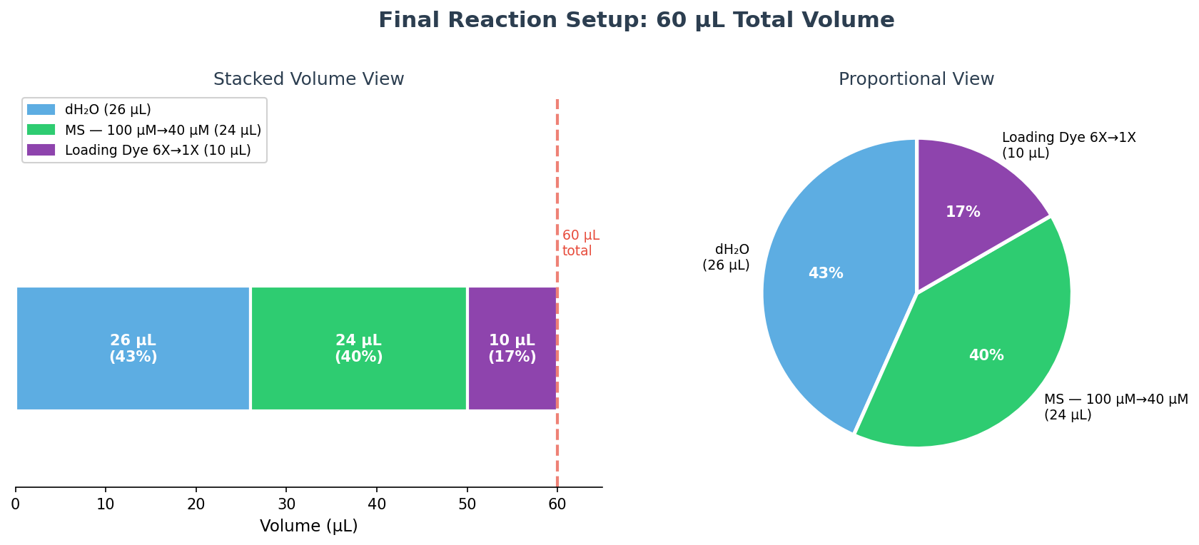
Part c — Final reaction table (60 µL total)

Using C₁V₁ = C₂V₂ for each component:

• Loading dye: V₁ = (1X × 60 µL) / 6X = 10 µL
• MS: V₁ = (40 µM × 60 µL) / 100 µM = 24 µL
• dH₂O: 60 − 10 − 24 = 26 µL

Why prepare 100 µM if 40 µM is the target?

Serial dilutions work most reliably when each step uses a round dilution factor (e.g., 1:500, 1:100) that keeps every transfer volume within the accurate range of an appropriate pipette. Diluting 5 M directly to 40 µM would require a 125,000× dilution — no two-step combination with round factors produces this cleanly. By creating a 100 µM intermediate stock first, the dilution ladder stays simple (1:499 → 1:99), and the final 40 µM is achieved precisely in the reaction setup using the P20. A secondary benefit: the 100 µM stock can be re-used for additional experiments without repeating the full dilution from scratch.

Lab Documentation

Materials

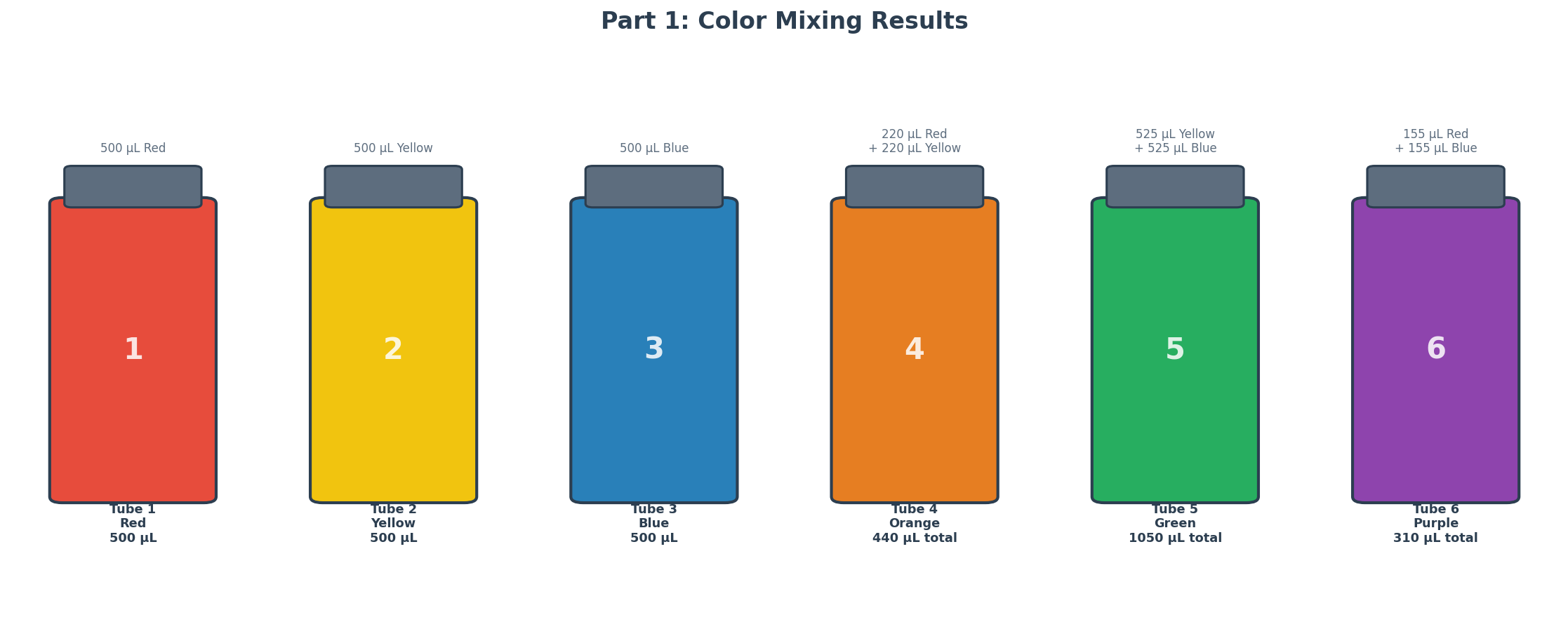
Part 1: Mixing Colors

Six numbered Eppendorf tubes were prepared using red, yellow, and blue food coloring solutions to explore color mixing and build volume intuition at different scales.

For Tube 4, the 220 µL of each color was added in two steps: 200 µL first (P200), then 20 µL (P20), with a tip change between colors to prevent cross-contamination. Mixing was done by pipetting up and down 3–4 times after each addition.

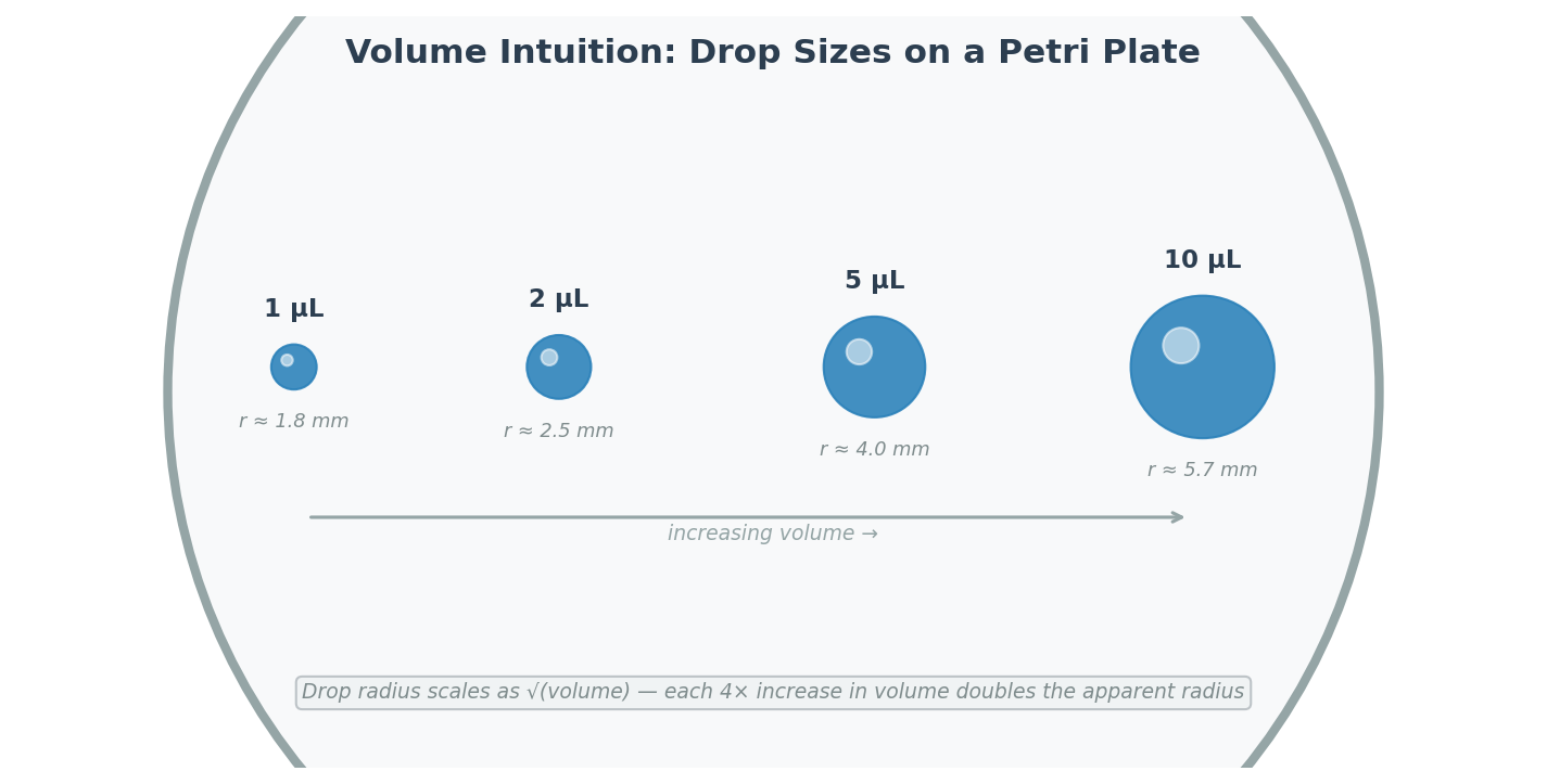
Small volumes of each solution were spotted onto a petri plate in increasing amounts (1 µL, 2 µL, 5 µL, 10 µL) to develop an intuitive sense of scale. At 1 µL, the drop is barely visible; at 10 µL, the drop is clearly a visible dome.

Part 2: Serial Dilution

The two-step protocol was followed to prepare a 100 µM working stock of MS from the 5 M stock, then combined into the final 60 µL reaction:

Step 1 (500× dilution): Using the P20, 1 µL of 5 M MS stock was transferred into a labeled Eppendorf tube. 499 µL of dH₂O was added with the P1000. The solution was mixed by pipetting up and down 4 times. The tube was labeled “10 mM MS”.

Step 2 (100× dilution): Using the P20, 10 µL of the 10 mM intermediate was transferred into a fresh Eppendorf tube. 990 µL of dH₂O was added with the P1000, mixed 4 times, and the tube was labeled “100 µM MS”.

Final Reaction Assembly (60 µL total):

Water was added first to reduce viscosity effects, then MS, then the concentrated loading dye last. The final reaction contains 40 µM MS and 1X loading dye in a bright purple solution.

Bonus — Gel Loading: 20 µL from the final reaction was pipetted into a pre-prepared agarose gel well. The tip was held just above the well opening (not inserted deeply) and the plunger depressed slowly and steadily to avoid puncturing the gel while ensuring the dense, dye-loaded solution sank into the well.

Week 2 Lab: DNA Gel Art

Gel Art: Restriction Digests and Gel Electrophoresis

Overview | Objective

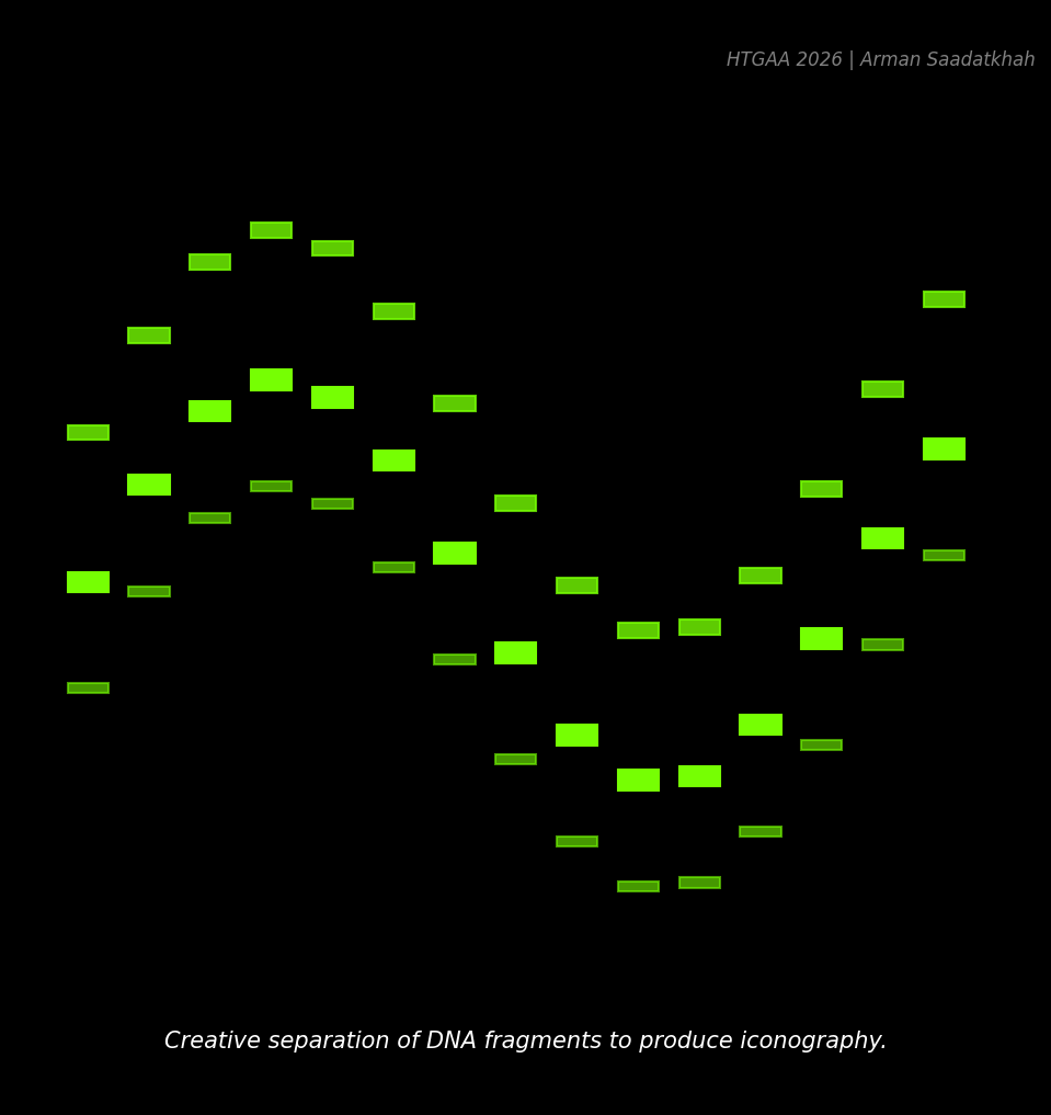
The goal of this 3-hour lab is to immerse you in the practical world of DNA gel electrophoresis and restriction enzyme-based DNA manipulation. You’ll create stunning DNA gel art while mastering essential techniques used in scientific research! Inspired by Paul Vanouse’s Art project and his Latent Figure Protocol, this lab offers a unique opportunity to blend creativity with molecular biology. By visualizing DNA fragments of varying lengths, you’ll gain firsthand experience in a process critical for verifying DNA sequences.

While the outcome of this lab is primarily artistic, gel electrophoresis is a fundamental tool in molecular biology for verifying DNA sequences. It allows you to confirm that the DNA you have obtained—whether purchased, purified, or constructed—matches your expectations. By comparing the lengths of DNA fragments observed on the gel to your predictions, you can assess whether the DNA sequence is correct. Although sequencing provides definitive confirmation, it is significantly more expensive, making gel electrophoresis an essential and cost-effective preliminary step in DNA analysis.

“The America Project”, Paul Vanouse, 2016. (Simulated iconographic Gel Art)

Overview | Concepts Learned & Skills Gained

This lab aims to enhance your understanding of core molecular biology concepts, including the mechanism of gel electrophoresis, the function of restriction enzymes, and the interpretation of DNA banding patterns. Through hands-on experience, you will gain skills in:

• Benchling Tools: Importing and analyzing DNA sequences, simulating restriction digests, and designing gel layouts.
• Restriction Digest Setup: Preparing precise enzyme reactions for targeted DNA fragment generation.
• Agarose Gel Preparation: Calculating and casting 1% agarose gels with appropriate buffers and DNA stains.
• Gel Electrophoresis Execution: Loading samples with accuracy, setting up electrophoresis apparatus, and troubleshooting common issues.
• DNA Visualization: Using a blue light transilluminator to image and document gel results effectively.

Pre-Lab | Reading

(1) How does Gel Electrophoresis Work?

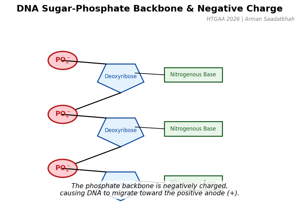
In gel electrophoresis, we place DNA samples in a semi-solid gel called agarose. The gel acts as a molecular mesh. DNA has a negative charge due to the phosphate groups in its sugar-phosphate backbone. When placed in an electric field, DNA fragments move towards the positively charged electrode (the anode).

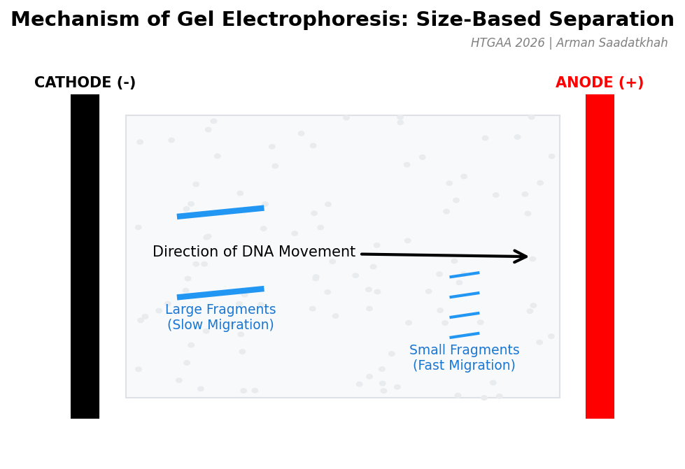
When an electric current is applied, the DNA fragments are pulled through the gel. However, their movement is influenced by size:

• Smaller DNA fragments navigate through the pores more easily and move faster toward the anode.
• Larger DNA fragments experience more resistance, slowing their progress.

(2) DNA Gel Ladders

Gel electrophoresis separates DNA fragments based on length only. DNA Ladders serve as molecular weight markers (biological rulers) providing standardized DNA sizes for comparison.

(3) Restriction enzymes

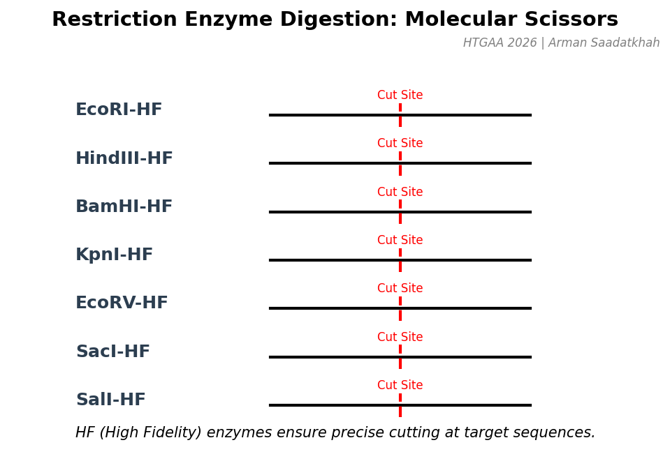
Restriction enzymes, or endonucleases, cut DNA at specific sequences called restriction sites. Each enzyme recognizes a unique nucleotide sequence, often palindromic. We used High Fidelity (HF) enzymes for precision.

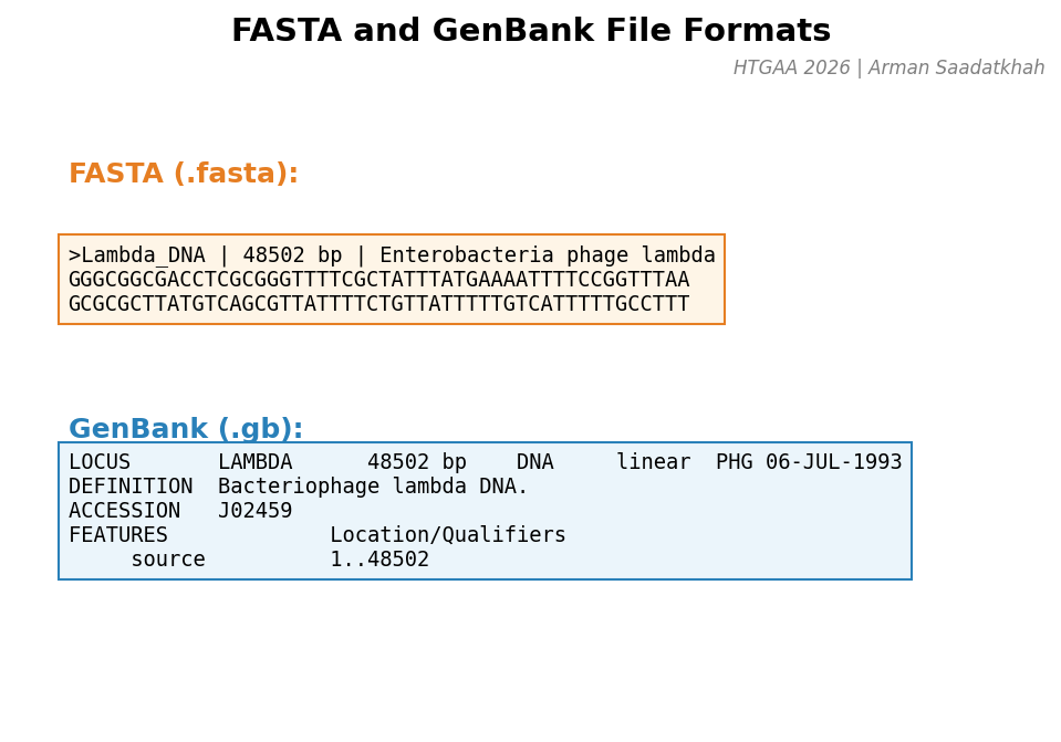
(4) GenBank and FASTA file formats

To run a virtual digest, DNA sequences are stored in FASTA or GenBank file formats. FASTA files have a simple format (sequence ID followed by the sequence), while GenBank files contain additional annotations.

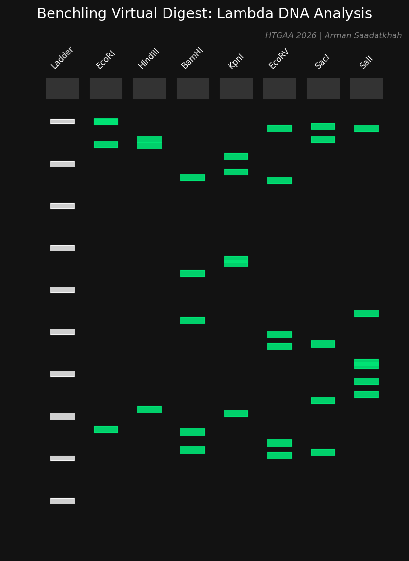
Protocol | Part 0: Designing your Gel Art

Time Estimate: 1 hour

Use Benchling to design your gel art and run your virtual digest. The distinct bands formed from gel electrophoresis can be used to create pictures.

Protocol | Part 1a: Preparing a 1% agarose electrophoresis gel

Time Estimate: 20 minutes prep, 30 minute wait

1. Add 0.75 g of agarose and 75 mL of 1x TAE buffer to a microwavable flask (1% w/v).
2. Heat in a microwave until dissolved.
3. Allow to cool to ~50 ºC, then add 7.5 μL of SYBR Safe DNA stain.
4. Pour into tray with comb and let solidify for 30 minutes.

Protocol | Part 1b: Restriction Digest

Time Estimate: 15 minutes prep, 20 minute wait

Protocol | Part 2: Gel Run

Time Estimate: 15 minutes setup, 1 hour wait

Loading the wells correctly is very important and requires a steady hand. Make sure the pipette tip hovers at the top of the well.

1. Load 20 uL of each sample into the wells.
2. Run the gel at 80V - 115V for around 45 minutes.

Protocol | Part 3: Imaging Your Results

Time Estimate: 5 minutes

Place the gel on the blue light transilluminator. Turn on the light, turn off room lights, and capture a clear image of the bands.

Supplemental | Troubleshooting

• Nonfunctional electrophoresis lane: Excessive DNA concentration or high voltage causing smearing.
• Bleeding trails: Human error in mixing or incorrect incubation.
• Samples not migrating: Check if water was used instead of TAE buffer (lack of conductivity).

HTGAA 2026 | Arman Saadatkhah | Reference: Paul Vanouse “The America Project”

Week 3 Lab: Opentrons Art

Opentrons Artwork: Fluorescent Bacteria Pixel Art

Overview | Objective

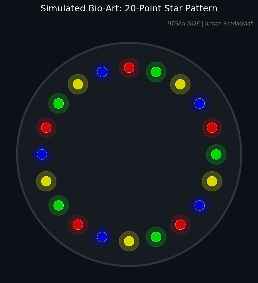
In this two-day lab, you’ll program the Opentrons OT-2 pipetting robot to create stunning, glowing designs by depositing genetically engineered E. coli onto black (charcoal) agar plates. These bacteria express fluorescent proteins in vibrant colors, forming “bio-art” that comes to life under UV light. It’s your chance to turn cutting-edge biotech into a canvas for creativity!

Fig 1. Simulated 20-point star pattern generated via Python for the Opentrons robot.

Overview | Concepts Learned & Skills Gained

This week, you will be working with the Opentrons OT-2, a liquid handling robot used in various life-science laboratories. You will learn:

• How to incorporate automation into synthetic biology research.
• How to code a Python script using the Opentrons API.
• How to create agar plates, a basic tool in molecular biology.

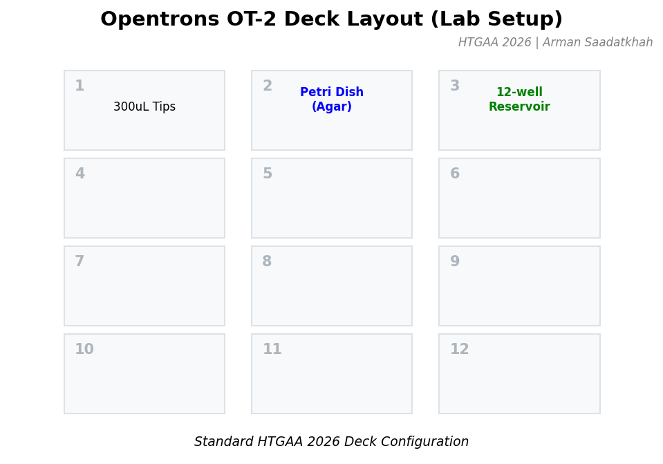
Fig 2. Standard HTGAA 2026 Deck Configuration for the OT-2 robot.

Pre-Lab | Reading

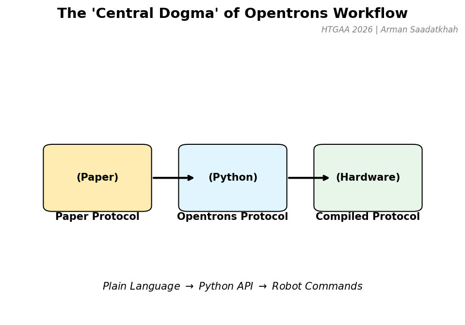
The “Central Dogma” of Opentrons

Before programming, it’s important to understand the workflow that transforms an idea into a precise robotic procedure.

Fig 3. The transformation from plain language instructions to hardware commands.

1. Paper Protocol: Instructions written in plain language (e.g., “Pipette 100 uL into A1”).
2. Opentrons Protocol: The Python script that translates these steps using the Opentrons API.
3. Compiled Protocol: The Opentrons App compiles the script into commands controlling the robot hardware.

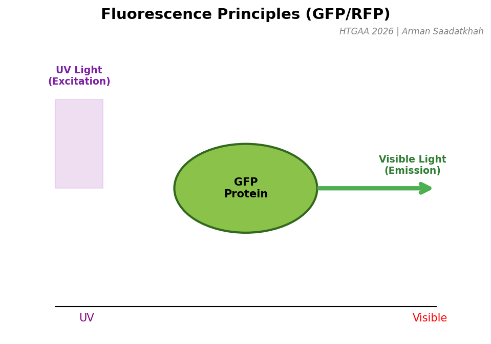
GFP and Friends: The Science of Glow

Green Fluorescent Protein (GFP) is a protein that glows green when illuminated with UV light. “Fluorescing” involves absorbing light at one wavelength (UV) and re-emitting it at another (Visible Green).

Fig 4. The mechanism of absorption and emission in fluorescent proteins.

For this lab, we use E. coli spliced with R/G/B/C/YFP genes. We mix charcoal powder into the agar to make it black, enhancing the visibility of the glowing designs.

Protocol | Part 1: Fluorescent Bacteria & Black Agar Script

Time Estimate: 2 Hours

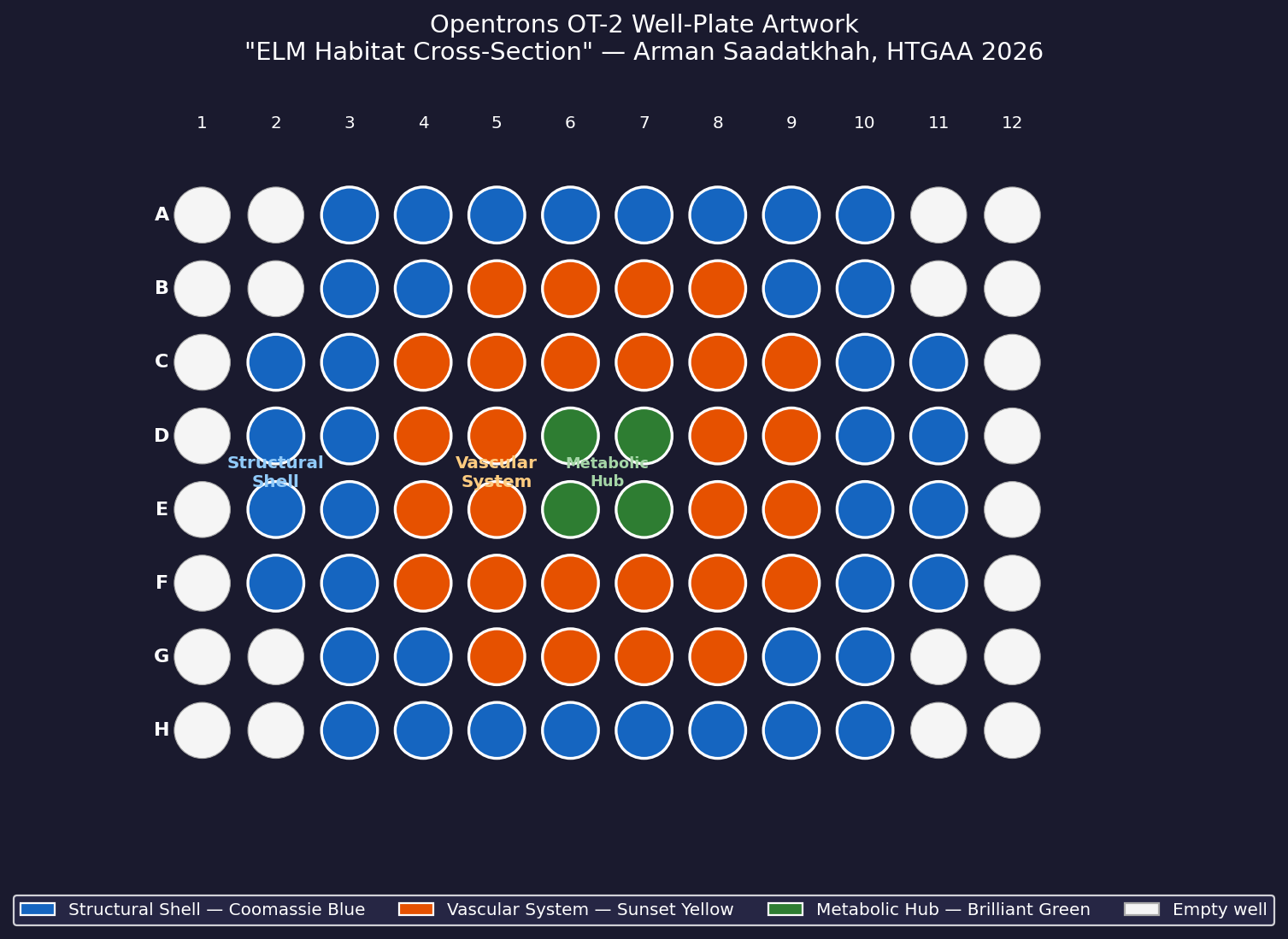
Artistic Concept — “ELM Habitat Cross-Section”

My design uses the 96-well plate as a canvas to depict a cross-sectional schematic of the Multi-Trophic Myco-Foundry — the engineered living material (ELM) habitat proposed in Week 1.

Fig 5. Well-plate layout for “ELM Habitat Cross-Section.” Blue = Structural Shell, Orange = Vascular System, Green = Metabolic Hub.

Python Script (Opentrons API v2.14)

The robot run starts without any tips. Fresh tips are used for every color to prevent cross-contamination.

from opentrons import protocol_api
import math

# Metadata and Setup
metadata = {'protocolName': 'ELM Habitat Art', 'apiLevel': '2.14'}

# Well classification logic for concentric rings
def classify_well(ri, ci):
    d = math.sqrt((ri - 3.5)**2 + (ci - 5.5)**2)
    if d < 1.5:             return 'hub'
    elif 1.5 <= d < 3.0:   return 'vascular'
    elif 3.0 <= d <= 5.0:  return 'shell'
    return 'empty'

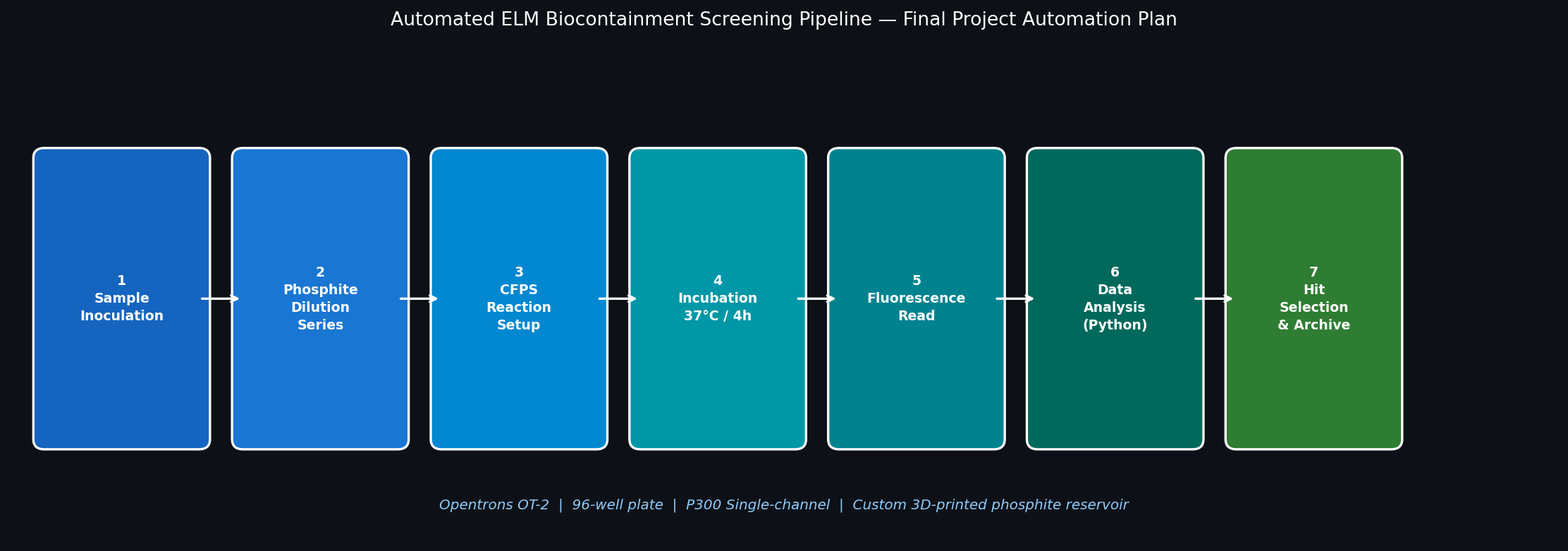
Protocol | Part 2: Automation Plan for Final Project

Goal: Use lab automation to screen and validate the phosphite auxotrophy biocontainment system.

Fig 6. Seven-step Opentrons automation pipeline for screening the ELM phosphite auxotrophy kill switch.

The OT-2 will run a 12-condition × 8-replicate growth screen, testing the ptxD-based kill switch across a 2-fold phosphite dilution series. This allows for rapid calculation of the IC₅₀ value, essential for the safety case of deployment.

Post-Lab | Troubleshooting & Results

Alice Cai’s final plate (2023) demonstrates the transition from a dark charcoal agar to a vibrant glowing masterpiece under UV light. Simple geometric shapes often yield the most precise results on the OT-2.

HTGAA 2026 | Arman Saadatkhah | Reference: Opentrons OT-2 Documentation

Week 6 Lab: Gibson Assembly

The Chromophore Color Cloning Quest

Overview | Objective

In this lab, you’ll be changing the color-generating chromophore of the purple Acropora millepora chromoprotein (amilCP) to a variety of orange, pink, and blue mutants.

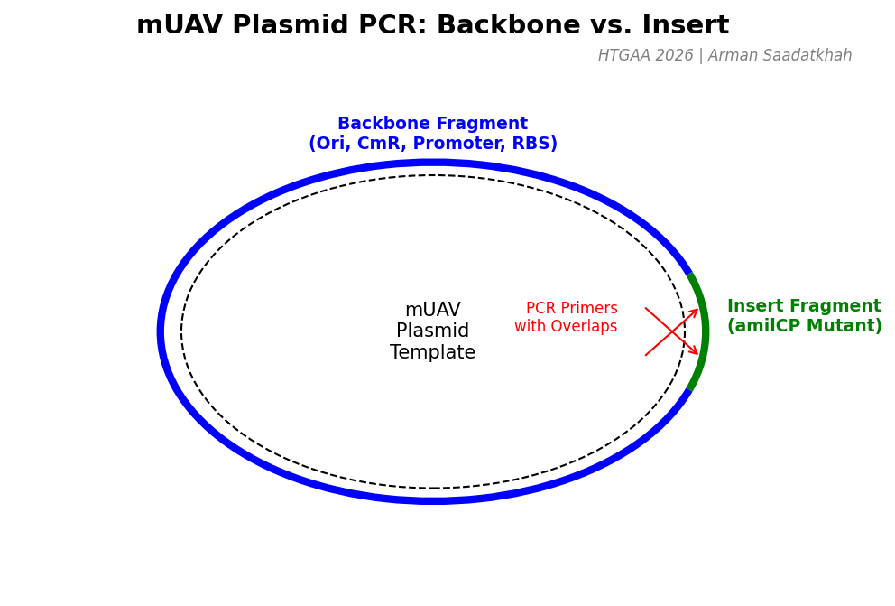
First, we’ll prepare two polymerase chain reactions (PCR) to generate the necessary fragments for a Gibson assembly. Using the amilCP-encoding Addgene mUAV plasmid as a template, we will amplify:

• The Backbone Fragment: Containing the origin of replication, Chloramphenicol resistance, and the promoter/RBS.
• The Insert Fragment: Containing the chromophore region with intentional mutations for color variation.

Fig 1. PCR strategy for generating Backbone and Insert fragments from the mUAV template.

Pre-Lab | Concepts

(1) Spectral Engineering of amilCP

The amilCP gene contains a chromophore (CP) region that can be mutated to express different colors. By changing the DNA sequence at the CP site (cagTGTCAGtac), we can engineer proteins that absorb light at different wavelengths.

Fig 2. DNA sequences and predicted phenotypes for various amilCP mutants.

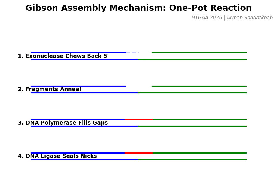
(2) Gibson Assembly Mechanism

Gibson Assembly is a “one-pot” isothermal reaction that allows multiple DNA fragments to be joined together. It relies on overlapping sequences (20-40 bp) at the ends of the fragments.

Fig 3. The four enzymatic steps of Gibson Assembly: Exonuclease chew-back, Annealing, Polymerase fill-in, and Ligase sealing.

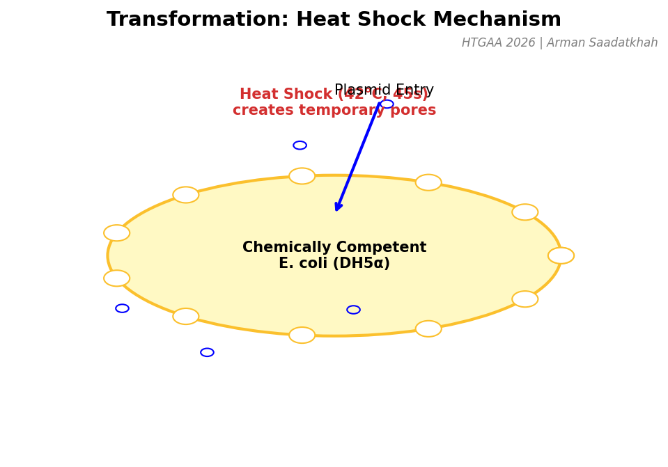
(3) Transformation

Once the plasmid is assembled, it must be introduced into E. coli cells. We use Heat Shock to create temporary pores in the cell membrane, allowing the DNA to enter by diffusion.

Fig 4. Mechanism of Heat Shock transformation in chemically competent DH5α cells.

Protocol | Part 1: PCR & Purification

PCR Setup

We set up two reactions to amplify the backbone and the mutant inserts.

• Backbone Fragment: ~2.5 kb (Primers: Backbone Fwd/Rev)
• Insert Fragment: ~0.5 kb (Primers: Color Fwd/Rev)

DpnI Digest & Purification

After PCR, we treat the samples with DpnI to digest the methylated template DNA (mUAV), ensuring only our newly synthesized mutant fragments are used in the assembly. We then purify the DNA using a silica-based column.

Protocol | Part 2: Assembly & Transformation

Gibson Assembly

We mix our purified Backbone and Insert fragments in a 1:2 molar ratio with the Gibson Assembly Master Mix and incubate at 50°C for 30 minutes.

Transformation

The assembled plasmids are transformed into DH5α competent cells.

1. Thaw cells on ice for 10 minutes.
2. Add 4 uL of assembly product.
3. Heat Shock: 42°C for exactly 45 seconds.
4. Outgrowth: Add SOC media and incubate at 37°C for 1 hour.
5. Plating: Plate onto LB + Chloramphenicol agar.

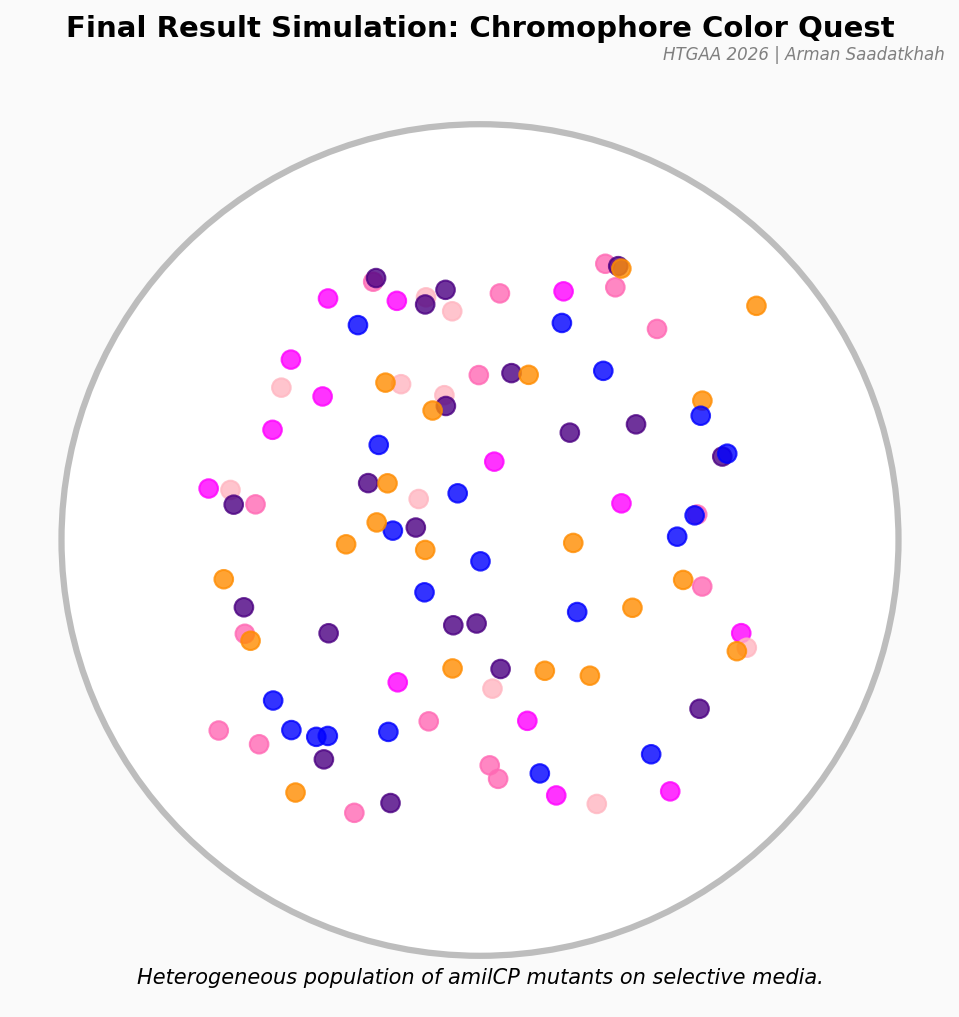
Final Results | Example

Fig 5. Predicted result showing a variety of colorful colonies representing different amilCP mutations.

After 72 hours of incubation, you should see a vibrant variety of purple, orange, pink, and blue colonies!

HTGAA 2026 | Arman Saadatkhah | Reference: Liljeruhm et al. (2018)

Week 7 Lab: Neuromorphic Circuits

Genetic Circuits II: Intracellular Artificial Neural Networks (IANNs)

Overview | Objective

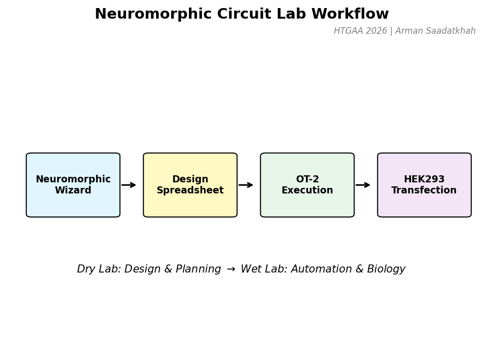
In this two-day lab, you will design and build your very own Intracellular Artificial Neural Network (IANN) using a library of plasmids from the Ron Weiss lab and human embryonic kidney (HEK) 293 cells.

Unlike traditional digital genetic circuits, IANNs perform analog computations and act as universal function approximators. Given an adequate number of intracellular artificial neurons (Sequestrons), you can use an IANN to achieve complex, non-linear input/output behaviors.

Fig 1. Laboratory workflow from computational design to automated execution and biological transfection.

Pre-Lab | Concepts

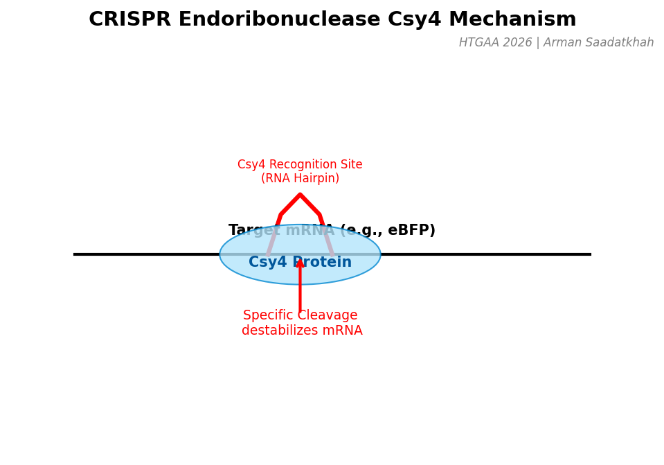
(1) CRISPR Endoribonucleases (Csy4)

Csy4 is a specialized CRISPR endoribonuclease that recognizes specific RNA hairpin sequences. In our circuit, Csy4 acts as the “neuron” that processes information by cleaving and destabilizing target mRNA (like eBFP), effectively performing analog subtraction or thresholding.

Fig 2. Schematic of Csy4 recognizing and cleaving a target mRNA recognition site.

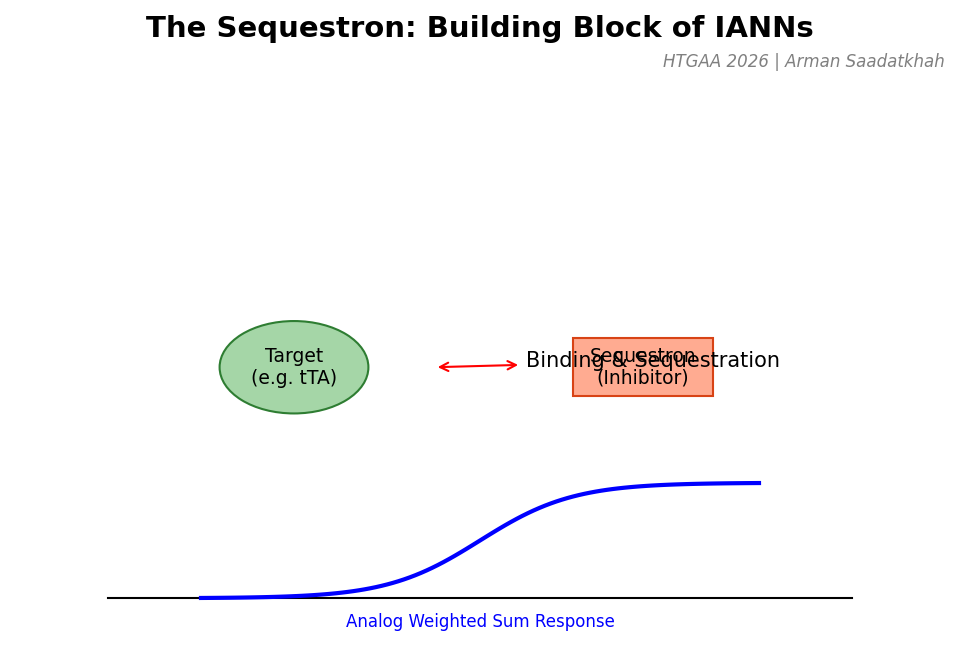
(2) The Sequestron

The Sequestron is the fundamental building block of neuromorphic genetic circuits. It works by “sequestering” or binding an activator (target) with an inhibitor (sequestron), creating a sharp, programmable analog response curve analogous to the activation functions in digital neural networks.

Fig 3. The Sequestron mechanism and its resulting analog weighted sum response.

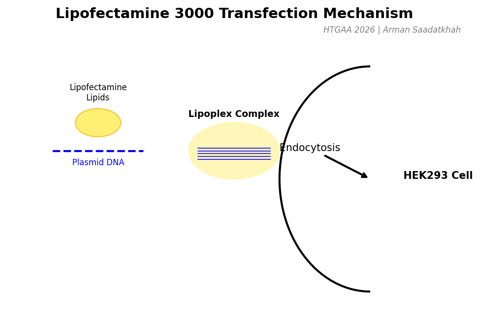
(3) Transfection with Lipofectamine 3000

To get our DNA designs into human HEK293 cells, we use Lipofectamine 3000. This reagent encapsulates plasmid DNA into lipid-based complexes (lipoplexes) that can easily enter cells via endocytosis.

Fig 4. Molecular mechanism of DNA-lipid complex formation and cellular entry.

Dry Lab | Neuromorphic Wizard & Design

The Neuromorphic Wizard software is used to predict the behavior of your IANN designs. By inputting different concentrations of Sequestrons and target plasmids, the wizard provides a simulation of the expected fluorescence output.

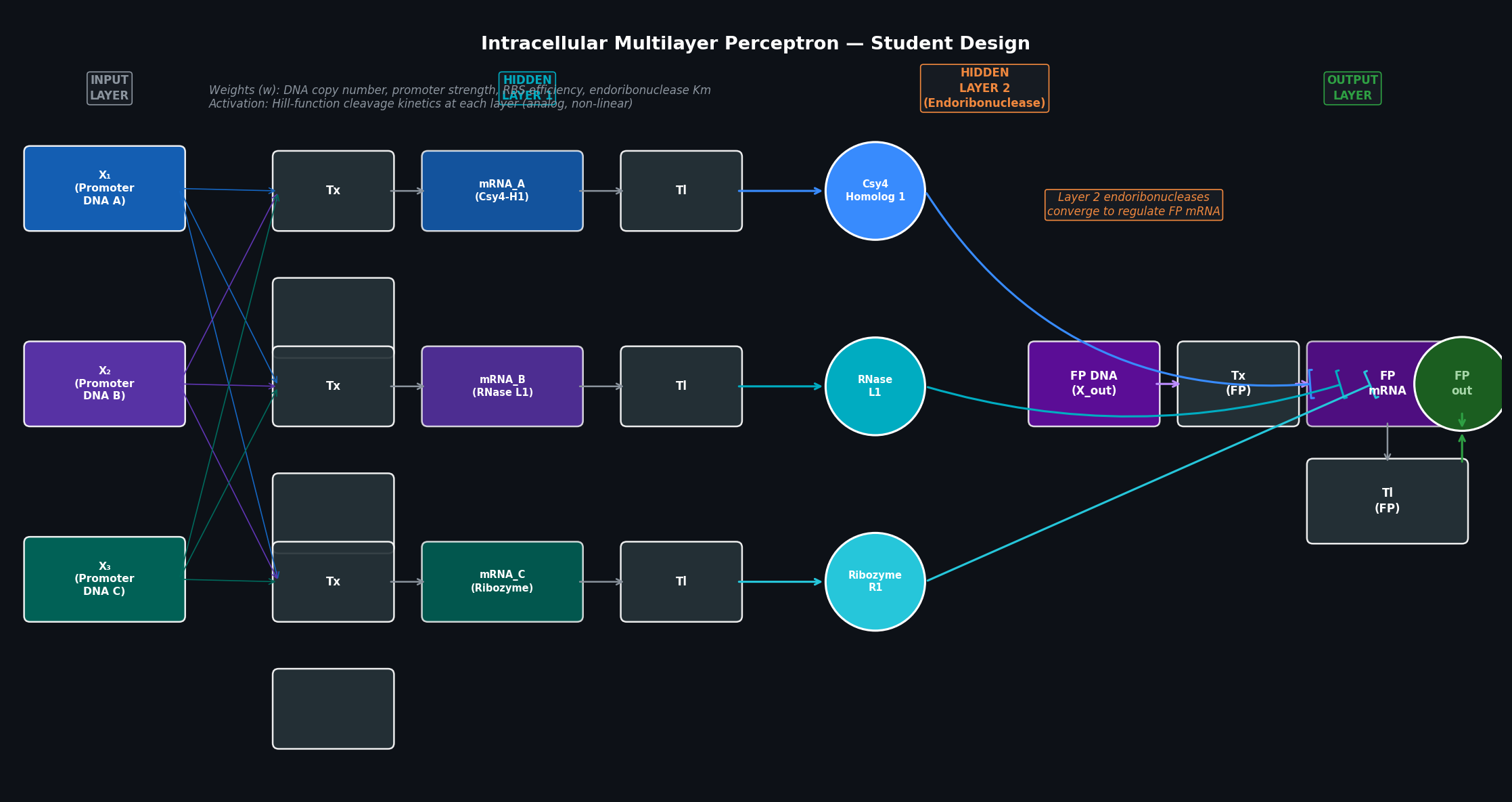
Multilayer IANN Design

For this lab, we developed a multilayer perceptron where multiple DNA inputs converge on a set of hidden layer neurons (endoribonucleases), which then regulate the final output protein level.

Fig 5. Multilayer intracellular perceptron design featuring hidden layers for complex signal processing.

Wet Lab | OT-2 Execution

The design is finalized in a Genetic Circuit Design Template (spreadsheet) and executed by an Opentrons OT-2. The robot handles the precise mixing of the plasmid library and the transfection reagents before adding them to the HEK293 cell culture.

Key Parameters:

• Concentration: 50 ng/μL
• Total DNA: Maximum 650 ng per circuit.
• Cell Type: HEK293 (Human Embryonic Kidney)

Results | Observation

Following transfection, the cells are incubated and observed for fluorescent protein expression. The graded intensity of the fluorescence across different wells validates the analog computational capability of the IANN.

HTGAA 2026 | Arman Saadatkhah | Reference: Ron Weiss Lab, MIT

Week 9 Lab: Cell-Free Systems

Cell-Free Transcription-Translation (TX-TL) Systems

Overview | What is Cell-Free?

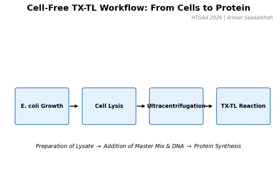
A cell-free system allows biological reactions to occur outside of living cells. By extracting and using cellular components like ribosomes, RNA polymerase, amino acids, and ATP, this method enables reactions in a controlled, simplified environment.

Fig 1. The general workflow for preparing and running a cell-free TX-TL reaction.

Applications

• Synthetic Biology: Testing circuits without cellular constraints.
• Protein Engineering: Rapid production of toxic or difficult proteins.
• Biosensing: Creating portable, paper-based diagnostic tools.

Technical Overview | TX-TL Production

A. Cell Extract Preparation

The process begins with E. coli growth, followed by washing and cell disruption (sonication or freeze-thaw). Ultracentrifugation at 30,000g separates the necessary machinery (ribosomes, factors) from debris. A strict cold chain is maintained to prevent enzymatic degradation.

B. Master Mix Components

The master mix provides the chemical environment and energy required for synthesis.

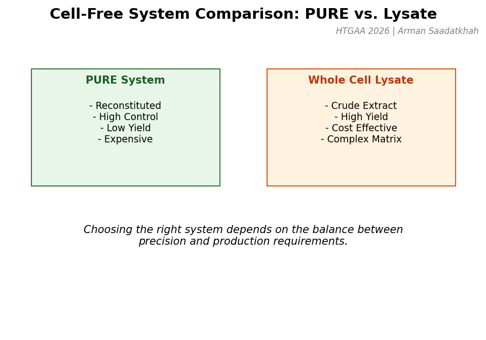
System Comparison | PURE vs. Lysate

There are two primary types of cell-free systems: the PURE System (defined, purified components) and Whole Cell Extract (crude lysate).

Fig 2. Comparison between the PURE system and Whole Cell Lysate systems.

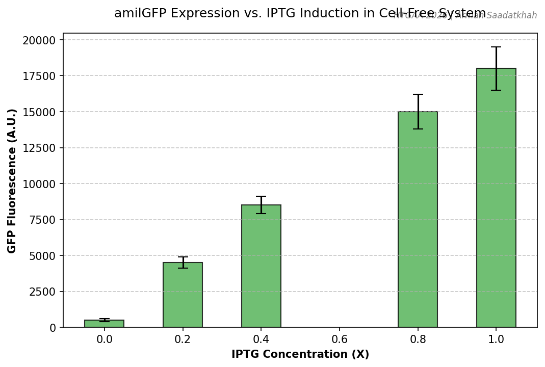
Lab Exercise | amilGFP Induction Quest

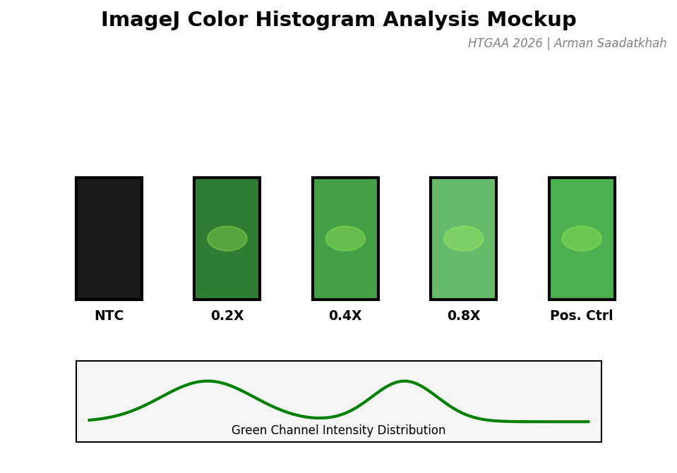
The objective of this lab was to quantify protein production in a cell-free extract using different IPTG levels to induce the expression of amilGFP from a T7-IPTG-inducible plasmid.

Results & Analysis

Fluorescence was monitored over an 8-hour incubation at 30°C. We analyzed the final-point results using ImageJ Color Histogram Analysis.

Fig 3. Mockup of the color histogram analysis used to quantify GFP expression levels.

Fig 4. Quantified GFP fluorescence across varying IPTG inducer concentrations.

Observations

• Fold Change: We observed a significant dose-response relationship between IPTG concentration and GFP yield.
• Background: The Non-Template Control (NTC) showed minimal background fluorescence, validating the specificity of the T7-IPTG system.

Homework Questions

1. Advantages of Cell-Free Protein Synthesis

Cell-free systems offer unparalleled flexibility because the reaction is directly accessible. You can add non-canonical amino acids, adjust magnesium concentrations mid-run, or introduce toxic components that would kill a living cell.

• Beneficial Case 1: Toxic Proteins. Expressing antimicrobial peptides that would lyse the production host.
• Beneficial Case 2: Rapid Prototyping. Testing 100+ genetic circuit variants in a single day without the time-consuming transformation/cloning cycle.

2. Main Components and Roles

• Extract: Contains the molecular hardware (ribosomes, tRNA synthetases, RNA polymerase).
• Master Mix: Provides the fuel (ATP/GTP) and chemical environment (buffers, ions).
• Template (DNA): The software/instructions for the specific protein to be synthesized.

3. Energy Regeneration

Energy regeneration is critical because the initial ATP/GTP supply is exhausted within minutes. We use secondary energy sources like 3-PGA or PEP which, through the action of metabolic enzymes in the lysate, phosphorylate ADP back into ATP, ensuring a continuous supply for several hours.

4. Prokaryotic vs. Eukaryotic Systems

• Prokaryotic (E. coli): High yield, fast, and simple. Ideal for producing amilGFP or other reporter proteins.
• Eukaryotic (Wheat Germ): Slower but capable of complex Post-Translational Modifications (PTMs). Ideal for producing human signaling proteins like Insulin or complex antibodies that require chaperones for correct folding.

5. Optimizing Membrane Protein Expression

I would design the experiment by adding nanodiscs or synthetic liposomes directly to the cell-free reaction.

• Challenge: Membrane proteins are hydrophobic and aggregate in aqueous buffers.
• Solution: The presence of a lipid bilayer allows the protein to co-translationally insert into a stable environment, mimicking its natural state.

6. Troubleshooting Low Yield

• Reason 1: Template Degradation. Strategy: Increase concentration of Murine RNase Inhibitor or use a circular plasmid instead of linear PCR product.
• Reason 2: Substrate Depletion. Strategy: Perform the reaction in a dialysis format to continuously supply small molecules (NTPs, amino acids) and remove byproducts.
• Reason 3: Incorrect Mg2+ Concentration. Strategy: Perform a magnesium titration (e.g., 4mM to 16mM) to find the specific optimum for the T7 polymerase and ribosome used.

HTGAA 2026 | Arman Saadatkhah | Reference: TX-TL Laboratory Manual

Week 10 Lab: Mass Spectrometry

Analytical Protein Characterization via LC-MS

Introduction and Background

Modern bioengineering relies on the ability to understand biological molecules with extraordinary precision. Liquid chromatography–mass spectrometry (LC-MS) is a cornerstone technique for protein characterization, revealing critical information about:

• Molecular Weight
• Protein Sequence
• Protein Folding and Structure

In this lab, we follow an analytical progression from intact protein analysis, through structural interrogation under native and denaturing conditions, to peptide-level sequencing of enhanced Green Fluorescent Protein (eGFP).

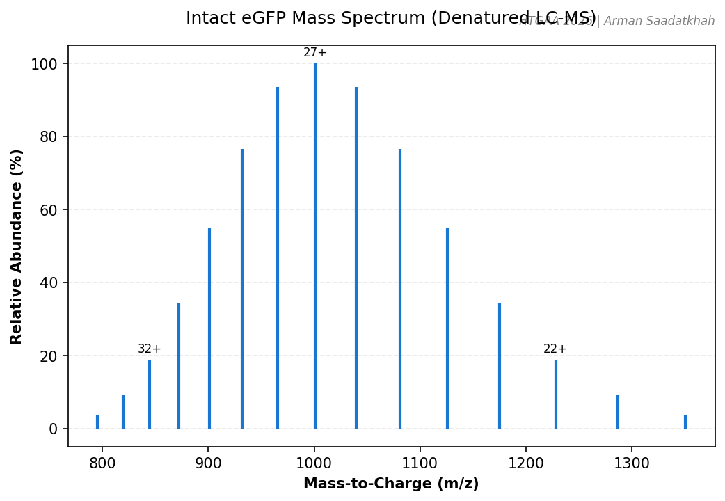
PART I: Molecular Weight Determination

Instrument: Waters Xevo G3 QTof

We analyzed an eGFP standard to determine its molecular weight based on mass-to-charge (m/z) and charge (z) measurements. Under denaturing chromatographic conditions, the protein unfolds, exposing protonation sites.

Fig 1. Simulated intact eGFP mass spectrum showing the charge state envelope (20+ to 34+).

Key Observations:

• eGFP MW: ~27 kDa.
• Deconvolution: MaxEnt1 was used to determine the observed molecular weight from the m/z peaks.

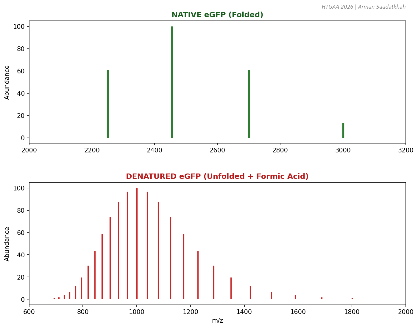
PART II: Native vs. Denatured Protein Structure

The higher-order structure of a protein influences its electrospray ionization (ESI) behavior.

• Native (Folded): Compact, fewer solvent-accessible sites, lower charge states (e.g., 9+ to 13+).
• Denatured (Unfolded): Elongated, many protonation sites, higher and broader charge states (e.g., 20+ to 40+).

Fig 2. Comparison of charge state distributions for native (folded) and denatured (unfolded) eGFP.

By adding formic acid to the native sample, we drop the pH and induce unfolding, directly observing the shift in the mass spectrum.

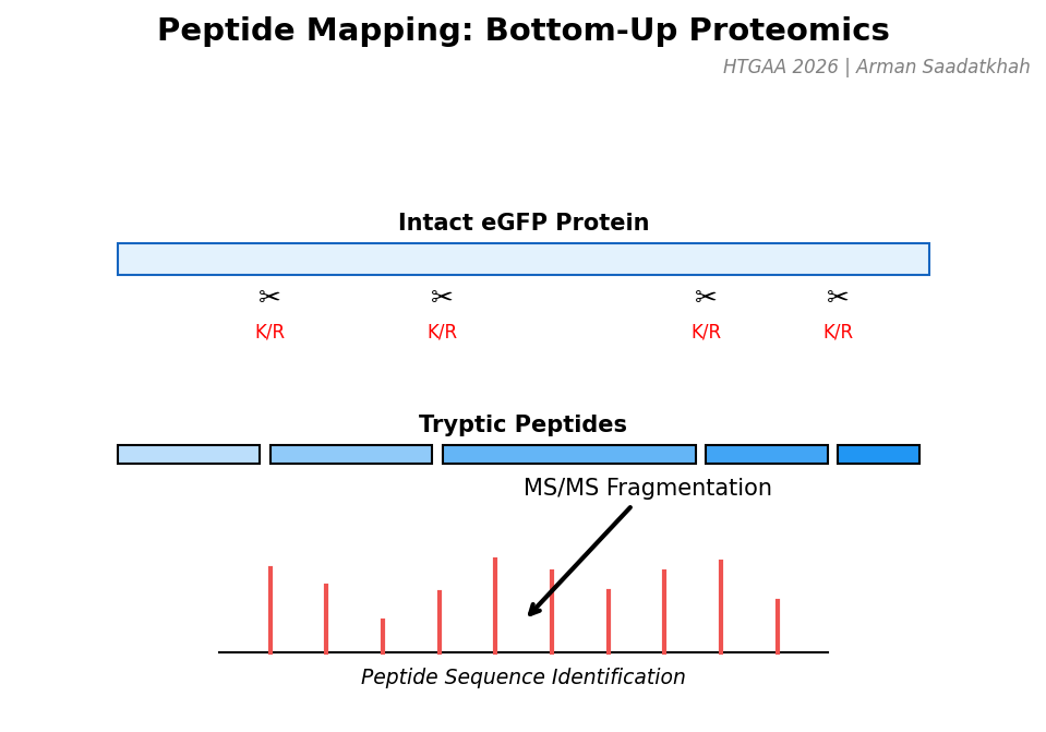
PART III: Peptide Mapping and Primary Sequence

Instrument: Waters BioAccord

To confirm the primary amino acid sequence, eGFP is enzymatically digested by trypsin, which cleaves at the C-terminal side of Lysine (K) and Arginine (R) residues.

Fig 3. Workflow for bottom-up proteomics: Digestion $\rightarrow$ Separation $\rightarrow$ Fragmentation (MS/MS).

Workflow:

1. Denaturation & Reduction: Guanidine HCl and DTT.
2. Buffer Exchange: Using BioRad Micro Bio-Spin columns.
3. Digestion: 20-minute incubation with RapiZyme Trypsin at 55°C.
4. LC-MS/MS: Fragmenting peptide ions to reconstruct the sequence.

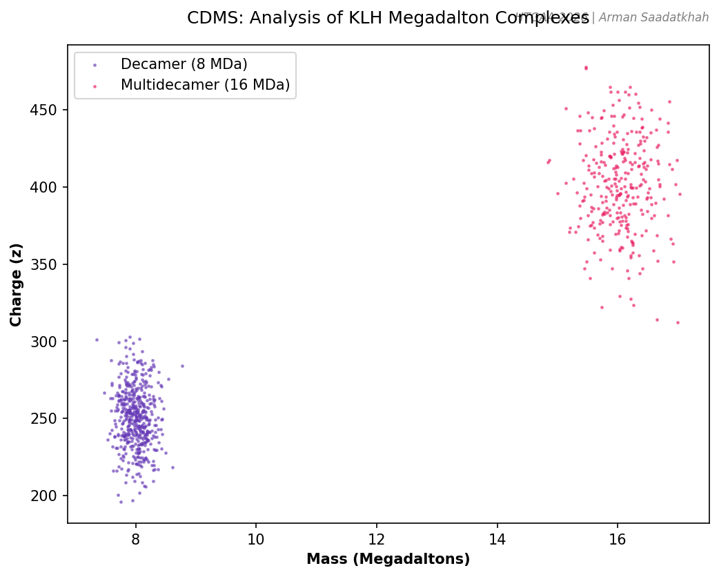
PART IV: Charge Detection Mass Spectrometry (CDMS)

Conventional MS struggles with megadalton-sized complexes due to unresolved charge states. CDMS enables the analysis of large complexes by measuring both m/z and charge (z) for individual ions simultaneously.

Analysis of Keyhole Limpet Hemocyanin (KLH)

KLH exists in massive oligomeric states, including decamers (~8 MDa) and multidecamers (12-32 MDa).

Fig 4. Simulated CDMS plot showing individual ions of KLH decamers and multidecamers.

HTGAA 2026 | Arman Saadatkhah | Reference: Waters Immerse Cambridge

Week 11 Lab: Introduction to Cloud Laboratories

Cloud Laboratories: Collective Art and Cell-Free Optimization

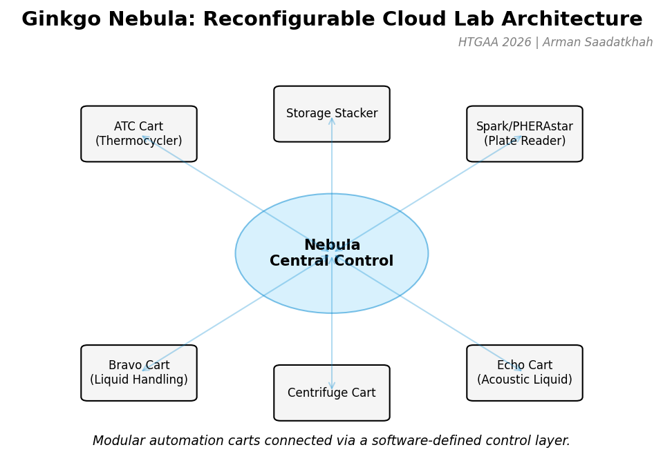
Overview | Introduction

Cloud laboratories are making science accessible, affordable, and reproducible. This lab showcases how cloud labs enable human creativity at scale and provide a platform for global collaboration. Our goal is to design a scientifically rigorous cell-free fluorescent protein optimization experiment together.

Fig 1. Ginkgo Nebula architecture featuring modular automation carts connected via a software-defined control layer.

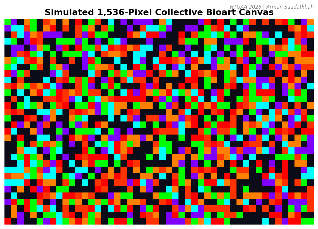
1. The 1,536 Pixel Artwork Canvas

The community bioart project involved contributing pixels to a global artwork experiment. This demonstrates the power of automation (Opentrons and Echo systems) to handle high-density layouts that would be impossible manually.

Fig 2. Simulation of the collective 1,536-pixel bioart canvas using various fluorescent proteins.

My Contribution:

• Pixel Location: I contributed to the “DNA” pattern on the bottom right plate.
• Reflection: I liked the seamless integration of individual designs into a unified biological canvas. For next year, real-time visualization of the design progress would be a great addition.

2. Cell-Free Protein Synthesis Reagents

A cell-free reaction requires a complex mixture of “hardware” (lysate) and “fuel” (master mix).

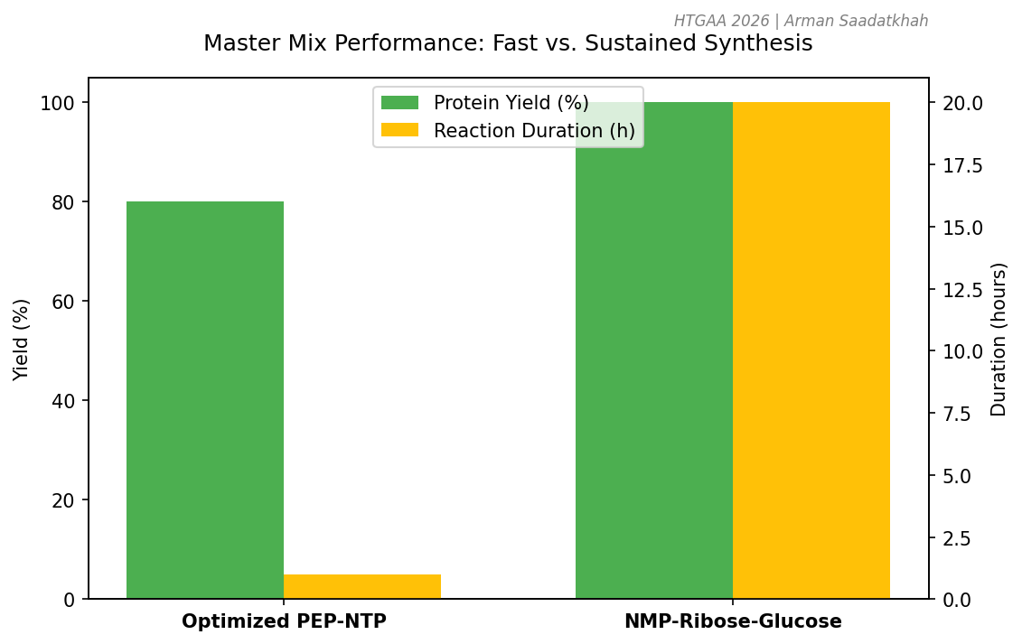
Master Mix Comparison

There are two main strategies for energy provision:

1. 1-hour PEP-NTP: Optimized for speed; uses high-energy phosphate donors (PEP) for rapid protein synthesis.
2. 20-hour NMP-Ribose-Glucose: Optimized for sustained production; uses secondary metabolism to regenerate ATP over longer periods.

Fig 3. Performance trade-offs between rapid (PEP-NTP) and sustained (NMP-based) energy systems.

Component Roles:

• BL21 (DE3) Star Lysate: The molecular machinery (ribosomes, tRNA synthetases, T7 RNA Polymerase).
• HEPES-KOH / Potassium Glutamate: Buffers and salts to maintain optimal pH and ionic strength.
• Ribose/Glucose/NMPs: Building blocks and energy precursors for sustaining the reaction.
• Guanine Bonus: Transcription can occur even without GMP if Guanine is present because the lysate contains salvage pathway enzymes (e.g., phosphoribosyltransferases) that can convert Guanine into GMP/GTP.

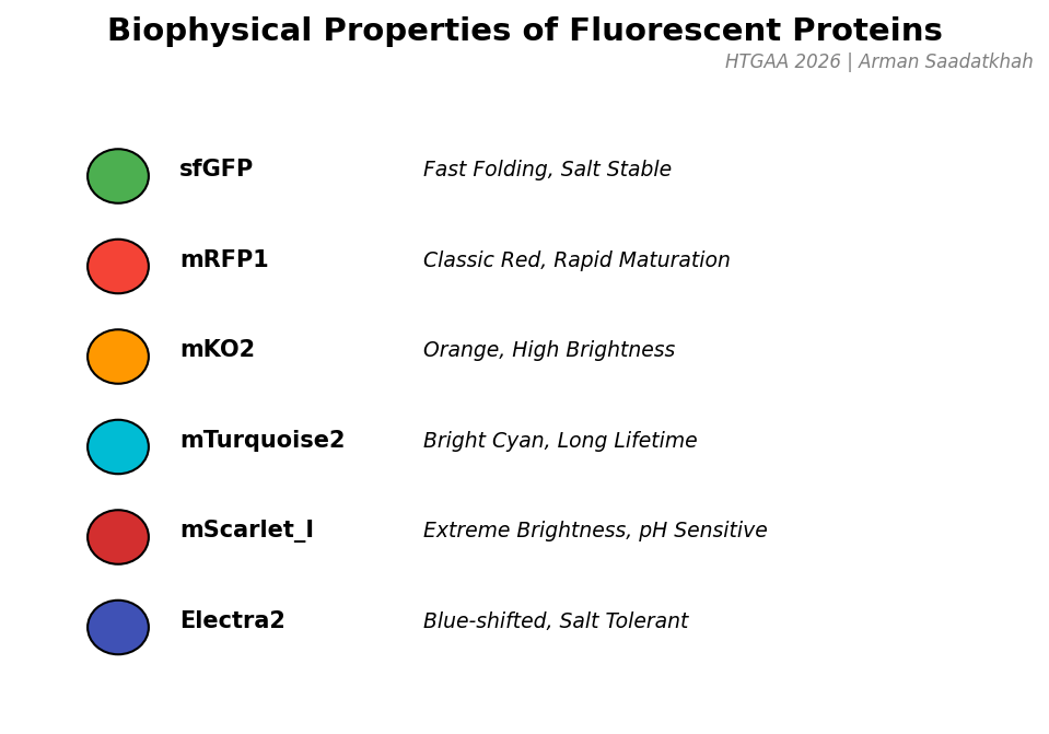
3. Global Experiment: Fluorescent Protein Properties

We used 6 different proteins for our collaborative painting, each with unique biophysical characteristics.

Fig 4. Key functional properties of the fluorescent proteins used in the collective optimization experiment.

Optimization Hypothesis:

• Target Protein: mScarlet_I
• Identified Property: High pH sensitivity (fluorescence drops in acidic conditions).
• Hypothesis: By increasing the HEPES buffer concentration in the master mix from 500mM to 750mM, we can maintain a more stable neutral pH as metabolic byproducts accumulate, thereby maximizing fluorescence over the 36-hour incubation.

4. Generic Cloud Lab Operations (JSON)

Automation in cloud labs like Ginkgo Nebula is driven by software-defined protocols. Below is a sample configuration for a spark_read operation:

{
    "spark_protocol_duration": 60,
    "bs_speed": 200,
    "pl_seal_temp": 166,
    "pl_seal_time": 2.5,
    "spark_protocol_steps": ["Fluorescence_Ex488_Em510"]
}

HTGAA 2026 | Arman Saadatkhah | Reference: Ginkgo Bioworks Nebula Platform

Week 12 Lab: Bioproduction of Beta-Carotene and Lycopene

Bioproduction of Beta-Carotene and Lycopene

Overview | Objective

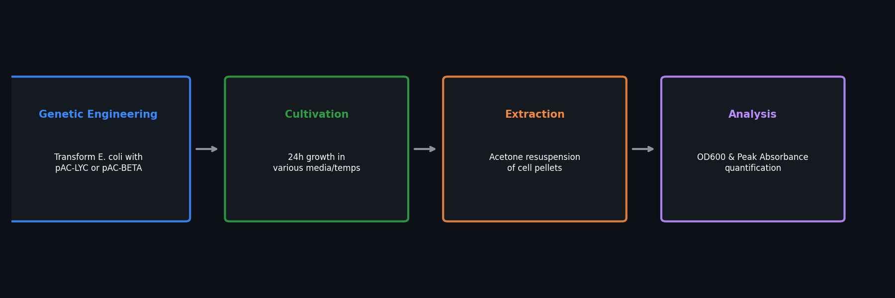
In this two-day lab, you will work with genetically modified E. coli to produce beta-carotene and lycopene, key plant pigments and antioxidants found in carrots and tomatoes. Using the plasmids pAC-LYC and pAC-BETA, which encode the pathways for lycopene and beta-carotene production, your goal will be to optimize the production of these two pigments.

This lab explores bioproduction, using biological systems—such as microorganisms (e.g., bacteria, fungi, algae) or plant and animal cells—to produce valuable compounds or materials. Bioproduction plays a critical role in various fields, including industrial biotechnology, pharmaceuticals, agriculture, and food production, enabling the creation of proteins, enzymes, antibiotics, biofuels, and more.

Fig 1. Overview of the bioproduction workflow, from genetic engineering to pigment extraction.

Overview | Concepts Learned & Skills Gained

A major challenge in bioproduction is the metabolic competition between the organism’s natural drive to reproduce and the production of the target compound. In this lab, you will explore how to fine-tune this balance to maximize pigment production, gaining hands-on experience in optimizing bioproduction systems.

You’ll investigate this by modifying culture conditions:

1. Temperature (30°C vs 37°C)
2. Growth Media Composition (LB vs 2YT, with and without fructose)

By examining how different environmental factors influence bacterial growth and synthesis, you will gain practical insights into metabolic engineering, advancing the potential for scalable bioproduction of essential compounds.

Pre-Lab | Reading

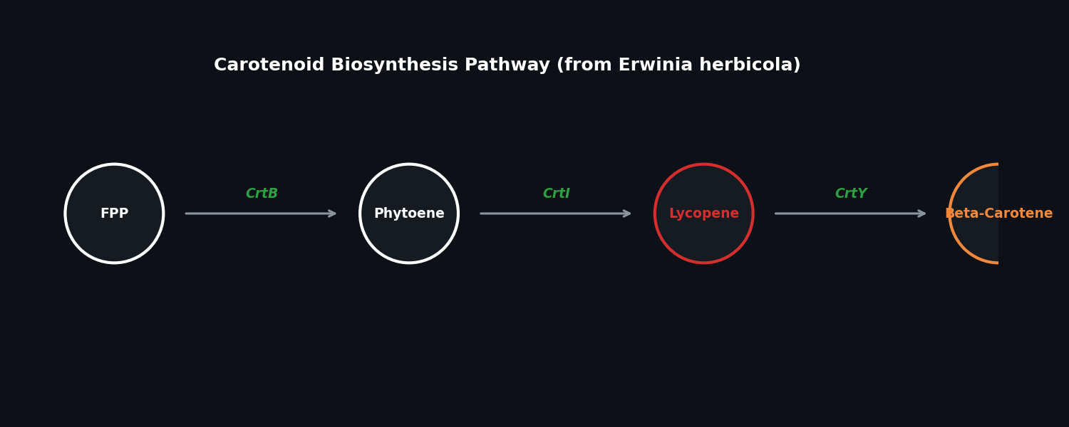
Referring to the pathway, lycopene is the red pigment that gives tomatoes their red color. This pigment is also made by microbes. In fact, transferring a 3-enzyme pathway to E. coli can convert farnesyl diphosphate (FPP) to lycopene.

Fig 2. The biosynthetic pathway for Lycopene and Beta-Carotene.

Plasmids

• pAC-LYC: Contains three genes from Erwinia herbicola: CrtE, CrtI, and CrtB. Produces lycopene.
• pAC-BETA: Produces beta-carotene through the addition of the Erwinia herbicola CrtY gene to the lycopene pathway.
• Resistance: Both plasmids include the gene for chloramphenicol resistance.
• Reference: Addgene #53270, #53272.

Optical Density (OD600)

We will be estimating cell growth by measuring the optical density of cells at a light wavelength of 600 nm (OD600). At 600 nm, dense cell suspensions scatter light, which correlates to approximate cell count. Always blank with the specified media first.

Pre-Lab | Safety

• Acetone: Review the Safety Data Sheet. Acetone is compatible with polypropylene (50 mL conical and 1.5 mL microcentrifuge tubes).

Protocol | Part 1: Overnight Cultures

Time Estimate: 30 Minutes setup, 24 Hour Incubation

Media, Equipment and Consumables

• LB and 2YT with chloramphenicol
• Fructose (for supplementation)
• Pipette set, serological pipettes, and tips
• Culture tubes
• Incubation room (30°C and 37°C)

Experimental Matrix (16 Conditions)

You will set up 16 unique conditions (plus duplicates and media controls, total 34 cultures).

Procedure

1. Prepare 3 mL of the specified media (supplemented with antibiotic).
2. Inoculate with 1 µL of E. coli starter culture containing the specified plasmid.
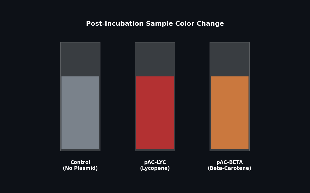
3. Grow for 24 hours in the circular roller drum at the appropriate temperature.

Fig 3. Expected color change post-incubation indicating pigment production.

Protocol | Part 2: Analyze OD600 and Peak Absorbance

Time Estimate: 180 Minutes

OD600 Measurement

1. Open the OD600 program on the spectrophotometer and blank with the respective media.
2. Measure using 800 µL of each culture in a cuvette.
3. Record values in an external table.

Pigment Extraction (Peak Absorbance)

1. Vortex the culture tube to ensure bacteria are suspended.
2. Transfer 1000 µL to a 1.5 mL microcentrifuge tube.
3. Centrifuge at 14,000 rpm for 1 minute.
4. Remove and discard the supernatant.
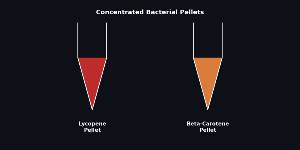
5. Repeat steps 2-4 two more times (total 3 mL concentrated into one pellet). Photograph the pellets!
6. Add 700 µL of acetone to the pellet and pipette up and down until resuspended. Acetone disrupts cell structure and solubilizes the carotenoids.
7. Centrifuge at 14,000 rpm for 1 minute.
8. Transfer 600 µL of the pigmented supernatant to a fresh tube.
9. Dilute with 600 µL of water (prevents acetone from corroding polystyrene cuvettes).
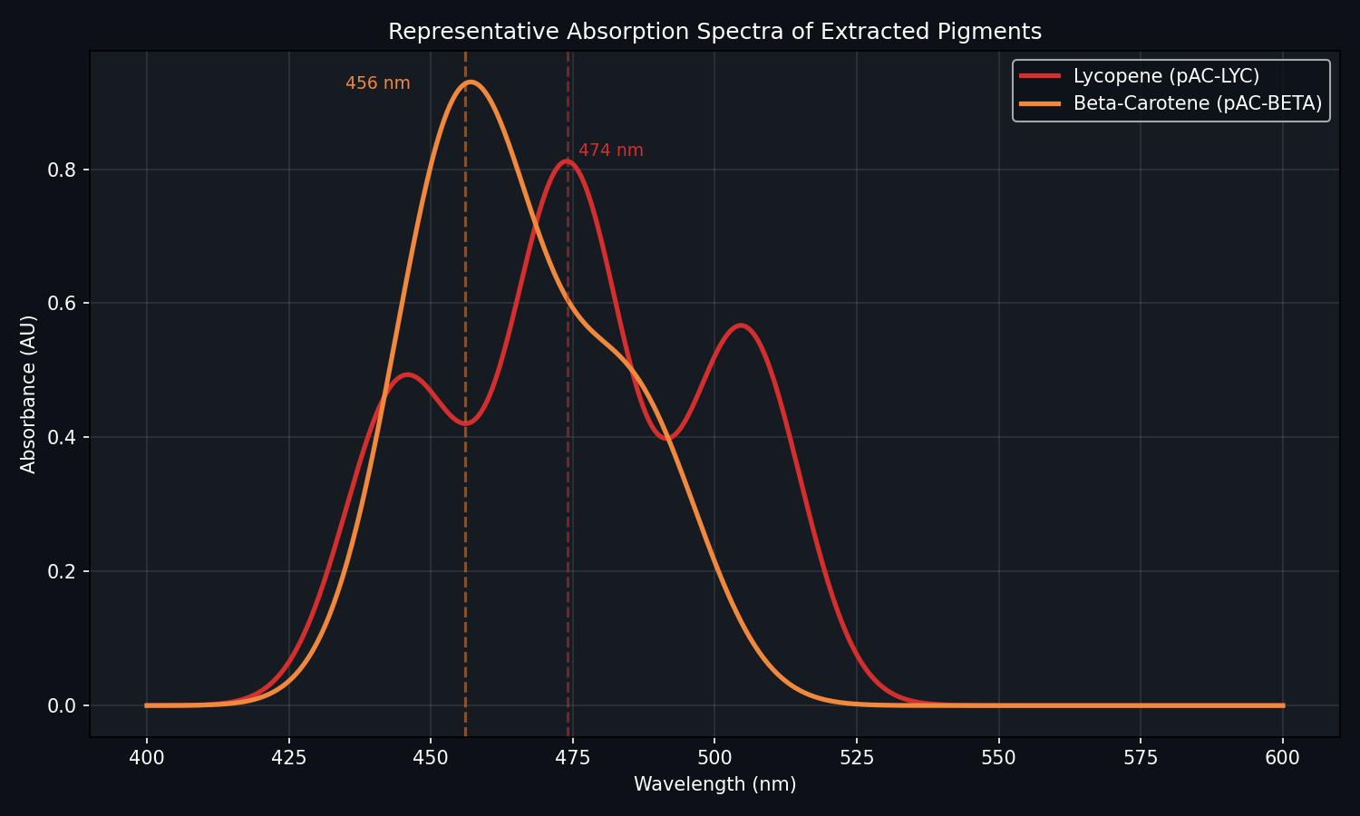
10. Measure absorbance on the spectrophotometer:
    • Lycopene: Measure at 474 nm.
    • Beta-Carotene: Measure at 456 nm.
11. Bleach samples and clean cuvettes after use.

Fig 4. Visualizing carotenoid accumulation in bacterial pellets.

Protocol | Part 3: Analysis

Time Estimate: 1 Hour

Compare relative pigment production per cell. Normalize each sample’s absorption peak measurement by its OD600 value.

• Which culture conditions led to the highest production?
• Plot your results using Excel or Python and include in your writeup.

Key Formula: Absorbance = 2 – log10(%Transmittance) (Beer-Lambert Law).

Fig 5. Example absorption spectrum. Note how pAC-BETA often performs better at 37°C.

Post-Lab Questions | Mandatory

1. Which genes when transferred into E. coli will induce the production of lycopene and beta-carotene, respectively?
   • Lycopene: CrtE, CrtI, and CrtB.
   • Beta-Carotene: CrtE, CrtI, CrtB, and CrtY.
2. Why do the plasmids need to contain an antibiotic resistance gene?
   • To provide a selective advantage to the transformed E. coli. Only bacteria containing the plasmid will survive on media supplemented with chloramphenicol, ensuring the population maintains the engineered pathway.
3. What outcomes might we expect when we vary the media, presence of fructose, and temperature?
   • Higher temperatures (37°C) typically increase growth rates but may lead to protein misfolding or metabolic stress. Nutrient-rich media (2YT) supports higher biomass than LB. Fructose provides an alternative carbon source that can bypass certain regulatory bottlenecks in the MEP pathway, potentially increasing pigment titer.
4. Generally describe what “OD600” measures and how it is interpreted here.
   • OD600 measures the turbidity (light scattering) of a culture at 600 nm. It is used as a proxy for cell density. In this lab, it allows us to normalize pigment production to the number of cells, ensuring we compare efficiency rather than just total volume.
5. What are other experimental setups where acetone could be used to separate cellular matter from a compound?
   • Extracting chlorophyll from leaves, isolating lipids from tissues, or precipitating proteins during DNA extraction.
6. Why engineer E. coli for this when Erwinia herbicola naturally produces them?
   • E. coli is a well-characterized “workhorse” with faster growth cycles, established genetic tools, and a lack of native pigments that would interfere with quantification. It allows for higher-scale, more controllable bioproduction.

Post-Lab Questions | For Committed Listeners Only

The following questions are based on supplemental readings and metabolic pathway design.

Metabolic Pathway Deep-Dive

1. Enzymes: What are the enzymes of the carotene pathway?
   • CrtE (GGPP synthase), CrtB (Phytoene synthase), CrtI (Phytoene desaturase), and CrtY (Lycopene β-cyclase).
2. Rate-Limiting Step: Which step takes the longest, and which enzyme is responsible for it?
   • Within the carotenoid pathway, CrtB (Phytoene synthase) is the primary rate-limiting enzyme. Globally in E. coli, the DXS enzyme (precursor supply) is often the major bottleneck.

DNA Construct Design

1. Organism Choice: Would you choose E. coli or S. cerevisiae for bioproduction? Why?
   • E. coli is preferred for rapid prototyping (20 min doubling time). S. cerevisiae (yeast) is preferred for food-grade products (GRAS) and has a superior native MVA pathway for precursor supply.
2. Expression Vector: Design an expression vector for E. coli. What parts are needed (RBS, terminators, operators, promoters)?
   • Required parts: Promoter (transcription start), Operator (regulation), RBS (translation initiation), Gene of Interest, Terminator (transcription stop), Selectable Marker (antibiotic resistance), and ORI (Origin of Replication).
3. Promoters:
   • What is the function of a promoter? To recruit RNA Polymerase to the DNA.
   • What is the difference between repressible and inducible promoters? Repressible are “on” until a signal turns them off; Inducible are “off” until a signal (e.g., IPTG) turns them on.
   • Which promoter would you use for a carotene/lycopene gene? Why? An inducible promoter (like pLac). This allows the culture to reach high biomass before “switching on” production, minimizing metabolic burden.
4. Origin of Replication (ORI):
   • What is an ORI? The site where DNA replication begins.
   • What are compatibility groups? Groups of plasmids that cannot coexist because they compete for the same replication machinery.
   • What is the best ORI for your chosen promoter and gene? A medium-copy ORI like p15A is often used for carotenoids to balance high yield with cellular health.

Advanced Engineering (Global Listeners)

1. Tuning: Elaborate on how RBS, terminators, and operators contribute to metabolic tuning.
   • RBS strength determines the protein concentration; Terminators prevent transcriptional read-through; Operators allow for dynamic control based on environmental signals.
2. Aptamers & Riboswitches: How can these be used for metabolic engineering in prokaryotes?
   • They act as RNA-based sensors that can sense product levels and automatically down-regulate or up-regulate expression to maintain optimal metabolic flux.
3. Assembly: What approach (e.g., Gibson, Golden Gate) would you use to join these parts?
   • Gibson Assembly for large, scarless constructs; Golden Gate for high-throughput modular library testing.
4. Dream Application: Elaborate on a biosynthetic pathway you would engineer in E. coli. What is its potential impact?
   • Engineering E. coli to produce Astaxanthin (a potent antioxidant) for sustainable aquaculture, reducing the need for synthetic dyes in the salmon industry.

Yeast Engineering (S. cerevisiae)

1. Integration: Create an integration cassette for homologous recombination.
   • Structure: [5’ Homology Arm] - [Promoter] - [Gene] - [Terminator] - [Marker] - [3’ Homology Arm].
2. Parts: List the eukaryotic-specific parts (e.g., Kozak sequence, terminators) needed.
   • Kozak sequence (ACC ATGG), Eukaryotic Promoters (pGAL1), and Eukaryotic Terminators (CYC1).
3. Site Selection: What chromosome site would you use for integration and why?
   • The HO locus is ideal as it is a “safe harbor” where integration does not disrupt essential cellular functions.

HTGAA 2025 | Lab Protocol: Bioproduction of Beta-Carotene and Lycopene