Week 1 HW: Principles and Practices

Application: Living Materials with Multicellular Computational Networks for Collective Sensing and Spatial Response

What is it?

I am interested in Computational Living Materials(CLMs): materials embedded with engineered cells that form cell-to-cell communication networks capable of collectively sensing, processing, and responding to environmental stimuli. Unlike existing engineered living materials that react passively to single inputs, it contain genetic logic circuits enabling the material itself to perform distributed spatial computation before producing an output response.

The Skin Analogy

The concept is inspired by how human skin processes touch. When you feel the difference between a pinprick and a palm press, it’s not because individual nerve cells are different but because of the pattern of activation across a network of communicating cells. Your skin doesn’t just sense but also computes spatially; the sensor and the processor are the same system.

Why do I care?

I am curious about the biomaterial equivalent. Cells embedded in a biomaterial substrate would sense their environment and share information with neighbors and collectively produce visible responses that represent processed information. The material includes the entire signal chain of sensor, processor, output into one living substrate. A local stimulus at one point would trigger a cascade that propagates outward, producing a coordinated response with cell-to-cell communication. Different cell populations can play different roles and multi-cell-type signal-processing networks could potentially perform noise filtering, edge detection, and signal amplification.

I work at the intersection of sensor technology, interaction design, and material fabrication. I’m drawn to the idea that computation doesn’t need silicon but emerge from living systems embedded in the materials around us. This could enable environmental monitoring surfaces, responsive architecture, wearable health interfaces, and entirely new categories of living interactive media.

Policy Goals

1. Enhance Biosecurity

   • Prevent repurposing for harmful applications
   • Ensure genetic designs are traceable

2. Protect the Environment

   • Prevent engineered organisms from escaping into natural ecosystems
   • Prevent gene transfer to wild microbial populations
   • Ensure safe degradation at end of life

3. Ensure Predictable Emergent Behavior

   • Ensure collective behaviors are testable and predictable
   • Prevent unintended behavioral drift from cell mutation

4. Promote Equity, Access & Transparency

   • Prevent biological IP concentration by few corporations
   • Promote open-source genetic designs
   • Require clear labeling of engineered living organisms in materials
   • Establish accountability for harm caused by material

Three Governance Actions

Option 1: Mandatory Dual Biocontainment Standards (Federal Regulatory)

Purpose: Currently, engineered living materials are developed under general lab biosafety rules (BSL-1/2). There are no specific regulations for deploying engineered organisms in materials outside the lab. Propose requiring two independent containment mechanisms: synthetic nutrient dependency & genetic kill switch.

Design: Administered through EPA (environmental release) and FDA (consumer products) using existing biotech frameworks. Manufacturers submit containment data showing organisms degrade within a set timeframe outside intended conditions. Inter-agency review panel evaluates.

Assumptions: Dual containment is achievable at scale (unproven for manufacturing); EPA/FDA have expertise to evaluate this new category (uncertain); lab-tested containment holds in real-world conditions (questionable).

Risks of Failure & “Success”: Too strict → bans development; too loose → inadequate protection. Even “successful” regulation may create false confidence: lab-tested containment may not hold in complex real environments. GMO crop regulation exists, yet gene flow to wild relatives has still occurred.

Option 2: Open-Source Biological Safety Consortium (Community Self-Governance)

Purpose: Top-down regulation often lags behind fast-moving technology. Propose voluntary consortium (modeled on iGEM’s Safety Committee or IETF internet standards) sharing safety standards and open-source containment genetic parts.

Design: “CLM Safety Certified” mark incentivizes membership. Insurance companies require certification for liability coverage. Funded by member dues and government grants (NSF/DARPA). Public registry of deployed organisms. Peer-reviewed safety audits.

Assumptions: Voluntary participation is sufficient (companies may resist open-sourcing); safety mark creates market pressure but public awareness of these materials is near zero; peer review is effective.

Risks of Failure & “Success”: Without legal enforcement, bad actors ignore standards. Dual-use dilemma: publishing how containment works also teaches how to defeat it. Open-source security helps defenders but also informs attackers.

Option 3: Mandatory Behavior Simulation Before Deployment (Government-Funded Technical Strategy)

Purpose: Collective behavior may not be predictable from individual cell specs. Propose mandatory computational simulation before deployment, similar to autonomous vehicle simulation testing.

Design: Agent-based computer models where each virtual cell follows its genetic circuit rules and communication logic. NIH/NIST funds open simulation platforms. Manufacturers must simulate behavior across environmental scenarios, including modeling how mutations over 100+ generations could alter collective behavior.

Assumptions: Models can accurately capture emergent biological behavior; evolutionary drift is somewhat predictable; simulation infrastructure is affordable.

Risks of Failure & “Success”: Inaccurate simulation models provide false confidence. Favors large companies with computational resources (equity problem). Over-reliance on simulation reduces investment in physical containment.

How do the options compare?

Prioritization and Trade-offs

Option 2 as Foundation, with Elements of Options 1 and 3

I would prioritize Option 2 (Open-Source Safety Consortium) as the primary governance framework, supplemented with targeted elements from the other two options.

Why Option 2 as the foundation: CLM technology is at developmental stage and heavy top-down regulation (Option 1) would likely stifle research before it can demonstrate its potential benefits. However, development should happen within a safety-conscious community framework. The open-source consortium has precedent in synthetic biology (iGEM’s safety practices, the BioBricks Foundation) and in technology broadly (IETF for internet standards, Linux Foundation for open-source software). It promotes both safety and equity simultaneously. would prioritize Option 2 (Open-Source Safety Consortium) as the primary governance framework, supplemented with elements from the other two options.

Supplemented with:

• From Option 1: As CLMs approach consumer deployment (likely 5-10 years away), formal regulatory standards should be developed in collaboration with the consortium. The consortium’s standards would inform regulation rather than being replaced by it. This staged approach mirrors how 3D printing governance evolved, early community self-governance followed by targeted regulation as the technology matured.
• From Option 3: The consortium should invest in developing open-source simulation tools for emergent behavior prediction, not as a mandatory gate, but as a shared design tool that helps researchers anticipate and avoid dangerous emergent behaviors during the design phase. Making simulation tools open and accessible avoids the equity problems of mandating them.

Key Trade-offs

The core trade-off is between safety and innovation speed. Option 1 maximizes safety assurance but minimizes innovation velocity. Option 2 maximizes innovation velocity but relies on voluntary compliance for safety. Hybrid attempt balances both by scaling governance intensity with technology maturity, light-touch community governance now, harder rules later when the stakes are higher.

A second trade-off is between openness and dual-use risk. Publishing open-source containment mechanisms helps everyone build safer materials but also helps bad actors understand how to defeat it. The benefit of openness outweighs the dual-use risk at this stage, because the technology is too immature, and the safety community benefits enormously from shared tools. This could change as the technology advances.

Audience Considerations

• Local (MIT/Cambridge): The MIT Institutional Biosafety Committee (IBC) should develop specific guidelines for research, including containment protocols for materials that might be taken outside the lab as final projects.
• National (NIH/NSF): Federal funding agencies should support development of open-source safety tools and simulation platforms, and require funded research to register with the proposed consortium.

Uncertainties

1. Can emergent behavior in CLMs be made reliably safe, or is unpredictability an inherent and irreducible feature of networked living systems?
2. Will the public accept living organisms in their everyday materials? Social acceptance may be a larger barrier than technical or regulatory challenges.
3. How will CLMs interact with natural microbial ecosystems in ways we cannot predict? The history of introduced species suggests we should be humble about our ability to predict ecological consequences.
4. As AI and biological computation converge, will CLMs raise questions about material “agency” that our current ethical frameworks are not equipped to handle? If a material makes a collective decision that harms someone, the question of responsibility may require entirely new ethical or legal frameworks.

References: Jacobson gene synthesis lecture (HTGAA Week 1, Slides 1-5: cell as computer, Slide 14: MutS error correction, Slide 35: genomically recoded organisms, Slide 45: molecular beacons, Slide 46: swigRNA sensors, Slide 59: bioFPGA); Pataranutaporn et al. “Living Bits” (AHs 2020); Oxman et al. “Hybrid Living Materials” (Adv. Funct. Mater. 2019); Basu et al. “Synthetic multicellular system for programmed pattern formation” (Nature 2005, Weiss Lab); DARPA Engineered Living Materials program; Walker et al. “Self-pigmenting textiles” (Nature Biotechnology 2024); Imperial College quorum sensing spatial computation (ACS Synth. Bio. 2024); Wang et al. “Engineering Microbial Consortia as Living Materials” (ACS Synth. Bio. 2024).

(AI Prompt: I’m interested in computational living materials where engineered cells communicate to collectively process information. Help me understand whether this is novel compared to existing engineered living materials, multicellular computation, and living bits research; What are the ethical and biosafety concerns specific to this development to be used outside of labs? Is it possible and help me develop specifc policy and goals; What is the iGEM safety model and how does it compare to IETF-style self-governance? Could something similar work for living materials? What is agent-based modeling in biology? Could it predict emergent behavior in multicellular systems? I need to score my governance options against my policy goals but I’m new to biology, can you help me evaluate which approaches are strongest for things like preventing gene transfer or ensuring traceability? What are the trade-offs between open-sourcing safety mechanisms and dual-use risk in synthetic biology?)

Week 2 Lecture Preparation

Homework Questions from Professor Jacobson:

Nature’s machinery for copying DNA is called polymerase. What is the error rate of polymerase? How does this compare to the length of the human genome. How does biology deal with that discrepancy?

Error rate of polymerase is 1:10⁶. Compared to the length of the human genome with 3.2 billion bases, it is roughly 3,200 errors per cell division. Biology deals with this through the error correction Mismatch Repair (MMR) System such as MutS repair system, additional DNA repair pathways such as Nucleotide excision repair, genetic code redundancy and diploid genomes.

(AI Prompt: what are ways of error correction biology uses to prevent mutations in the human genome beyond the polymerase’s built-in proofreading)

How many different ways are there to code (DNA nucleotide code) for an average human protein? In practice what are some of the reasons that all of these different codes don’t work to code for the protein of interest?

The average human protein is encoded by ~1,036 base pairs of DNA (slide 6). Since each amino acid is encoded by a codon of 3 nucleotides, this corresponds to 1,036 ÷ 3 ≈ 345 amino acids. There are roughly 3³⁴⁵ ways for a protein of 345 amino acids. In practice, most of those sequences won’t work because of mRNA folding, codon usage bias (cells prefer certain codons), and accidental creation of regulatory regions.

(AI prompt: why are there not 3³⁴⁵ ways to code for the protein in biological reality)

Homework Questions from Dr. LeProust:

What’s the most commonly used method for oligo synthesis currently?

Phosphoramidite chemistry column-based and silicon chip-based DNA synthesis.

Why is it difficult to make oligos longer than 200nt via direct synthesis?

In the chemistry synthesis as the open loop protection system, yield is dropping as the number of coupling increases. (1 - 1/N)^N and the error rate is fixed at 1 out of 100 which is 1% for each one to be correct. With 99% coupling efficiency per step, the yield for a 200nt oligo is 0.99²⁰⁰ ≈ 13% usable ones because the error rate is fixed but the chain keeps getting longer. The longer it gets the less usable ones in percentage due to exponential yield decay.

Why can’t you make a 2000bp gene via direct oligo synthesis?

The cost and error rate is really high. With the error rate of 1:10², 20bp out of 2000bp will have error on average. The probability of getting something usable without error is 0.99²⁰⁰⁰ which is essentially impossible.

Homework Question from George Church: [Lecture 2 slides]

What are the 10 essential amino acids in all animals and how does this affect your view of the “Lysine Contingency”?

The 10 amino acids that animals cannot synthesize and must obtain from their diet are PVT TIM HALL: Phenylalanine, Valine, Threonine, Tryptophan, Isoleucine, Methionine, Histidine, Arginine, Leucine, Lysine. The “Lysine Contingency” from Jurassic Park is for biocontainment: if the dinosaurs ever escaped the island, they’d die without their lysine supplements from the park staff. The Lysine Contingency does not make sense because animals including us cannot produce their own lysine but get lysine from their diet, which means that the dinosaurs can freely obtain lysine the way all animals do — eat lysine-containing plants or animals.

(AI prompts: please explain in detail what are the 10 essential amino acids in all animals and what do they do? What is “lysine contingency”?)

Week 2 HW: DNA Read, Write, & Edit

DNA Design Challenge

1. Choose Your Protein

I chose Reflectin A1, the structural protein found in squid skin that is responsible for their ability to dynamically change color and iridescence. Squid iridophores contain layers of reflectin that can shift what wavelengths of light they reflect by changing the protein’s conformation — essentially biological tunable thin-film optics. I’m interested in this because it represents a living material that produces a dynamic optical output as a visual response through intrinsic material properties rather than added pigments. Researchers have fabricated reflectin-based thin films that change color in response to chemical signals, which sits right at the intersection of my interests in materials, sensing, and interaction.

Protein sequence from UniProt (D3UA43) / NCBI (ACZ57764.1):

2. Reverse Translate

Using NCBI, I traced the protein back to its original DNA coding sequence: FJ824804.1 — the mRNA for Reflectin-like protein A1 from Doryteuthis pealeii.

The sequence starts with ATG (start codon) and ends with TAA (stop codon). It’s 1,053 base pairs long, which checks out: 350 amino acids × 3 bases per codon = 1,050, plus 3 for the stop codon.

3. Codon Optimization

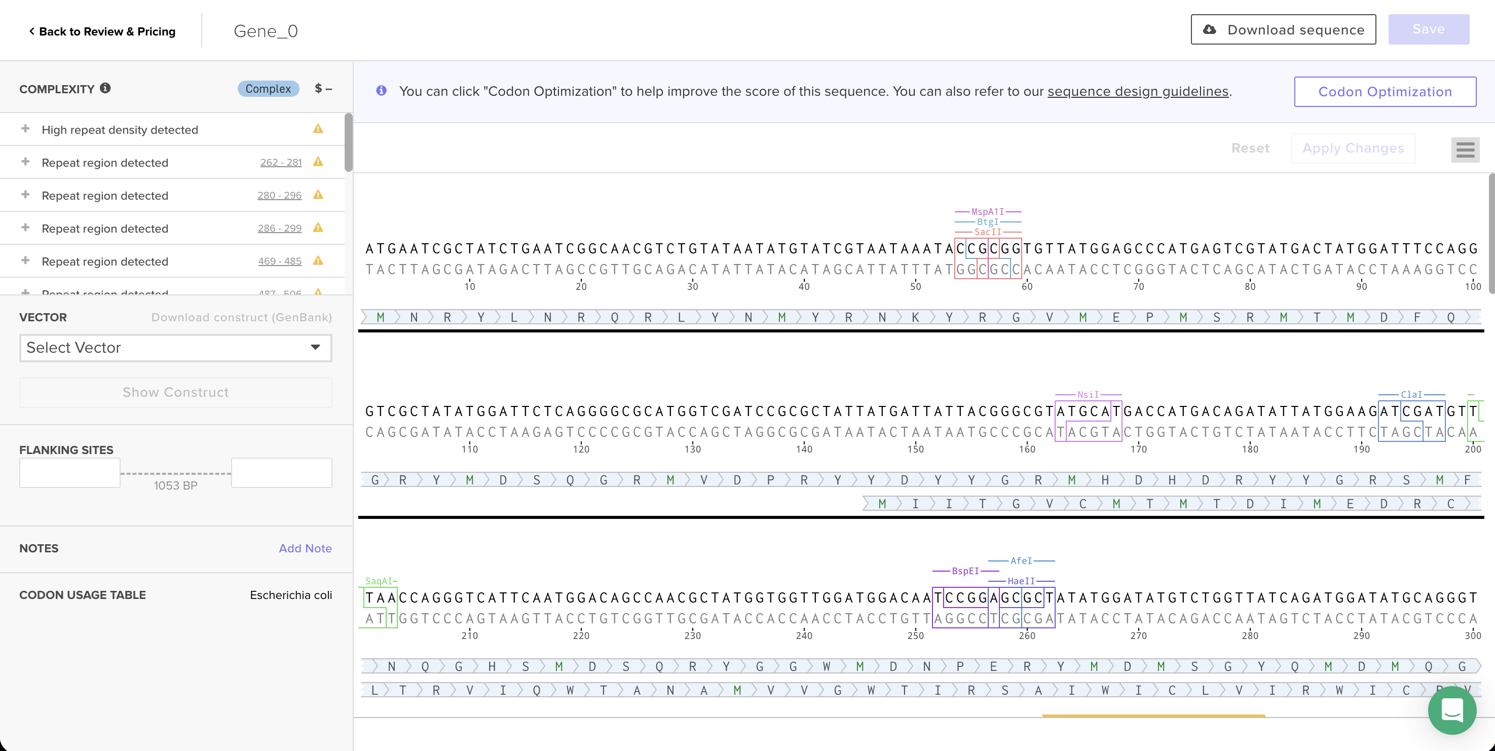
I optimized for E. coli because that’s the organism we’re using in the lab to express proteins. The original DNA sequence comes from squid, which uses a different set of preferred codons than E. coli. Even though multiple codons can encode the same amino acid, cells have different amounts of the tRNA molecules that read each codon. E. coli has abundant tRNA for its commonly-used codons and very little for rare ones. If I put the original squid DNA into E. coli, the ribosome would stall at codons that E. coli rarely uses, resulting in slow or unsuccessful protein production. Codon optimization swaps those squid codons for ones E. coli translates quickly, so it can produce it much more efficiently.

Codon-optimized sequence in Twist’s editor, with Codon Usage Table set to Escherichia coli.

Synthesis complexity: Twist flagged this sequence as “Complex” with 17 warnings — high repeat density and multiple repeat regions throughout the sequence. Reflectin’s amino acid sequence is highly repetitive (the motif YMDMSGYQMDMQGRWMD appears several times), and the underlying protein repetition still creates patterns that are hard to synthesize even after optimization. This is the same challenge the TAs described in recitation about spider silk proteins.

4. Producing the Protein

To produce reflectin from this DNA sequence, I would use a cell-dependent method by putting the DNA into living E. coli and letting them produce it:

• Expression cassette: The coding sequence needs to be wrapped with a promoter (“start transcribing here”), a ribosome binding site (so the ribosome knows where to land on the mRNA), and a terminator (“stop transcribing”).
• Insert into a plasmid: The expression cassette gets placed into a circular plasmid, which also carries an origin of replication (so the bacteria copy it when they divide) and an antibiotic resistance gene (to filter).
• Transform into E. coli: Using heat shock — the bacteria are chilled, the plasmid DNA is added, then a brief heat pulse causes temporary openings in the cell membrane allowing plasmids to enter. Cooled again to close the membrane.
• Grow: The bacteria are plated on media with antibiotics so only the ones carrying the plasmid (and its resistance gene) survive.
• Transcription and translation: The E. coli’s own RNA polymerase reads the DNA and creates mRNA (transcription). Then the cell’s ribosomes read the mRNA codons and build the reflectin protein chain using tRNA (translation).
• Protein: The bacteria are broken open to release the protein inside.

Prepare a Twist DNA Synthesis Order

1. Build DNA Insert Sequence

I built an expression cassette in Benchling by stitching together all the regulatory parts needed for E. coli to read and produce my reflectin protein. The parts, in order:

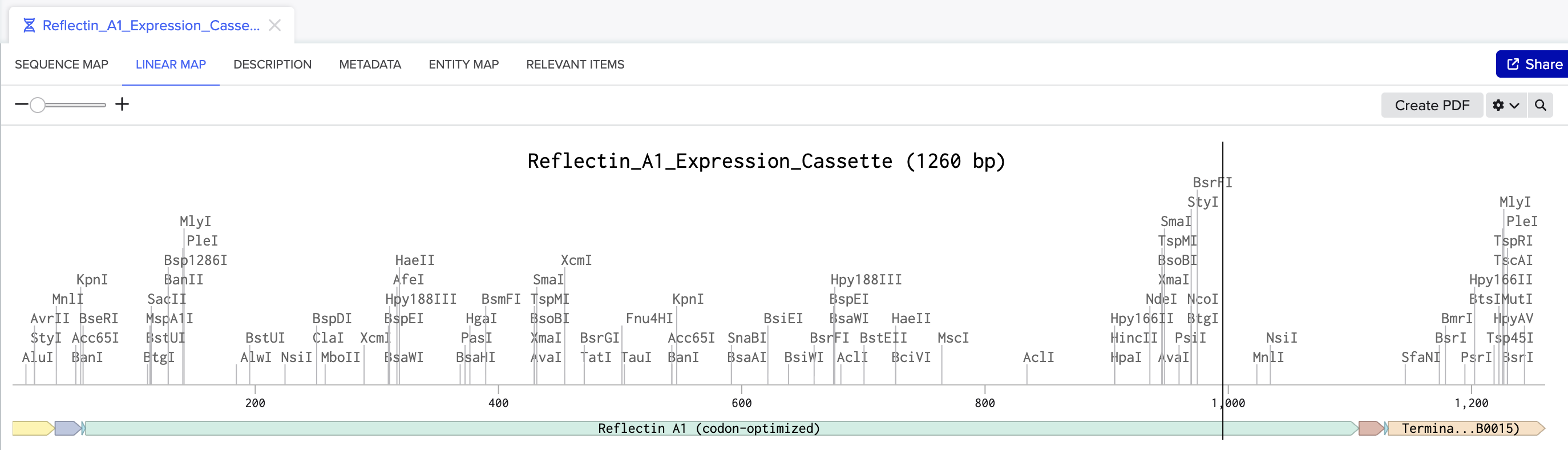
Linear map of the Reflectin A1 expression cassette in Benchling (1,260 bp), showing all annotated parts.

Benchling sequence link | Download FASTA | Download GenBank

2. Upload to Twist & Choose Vector

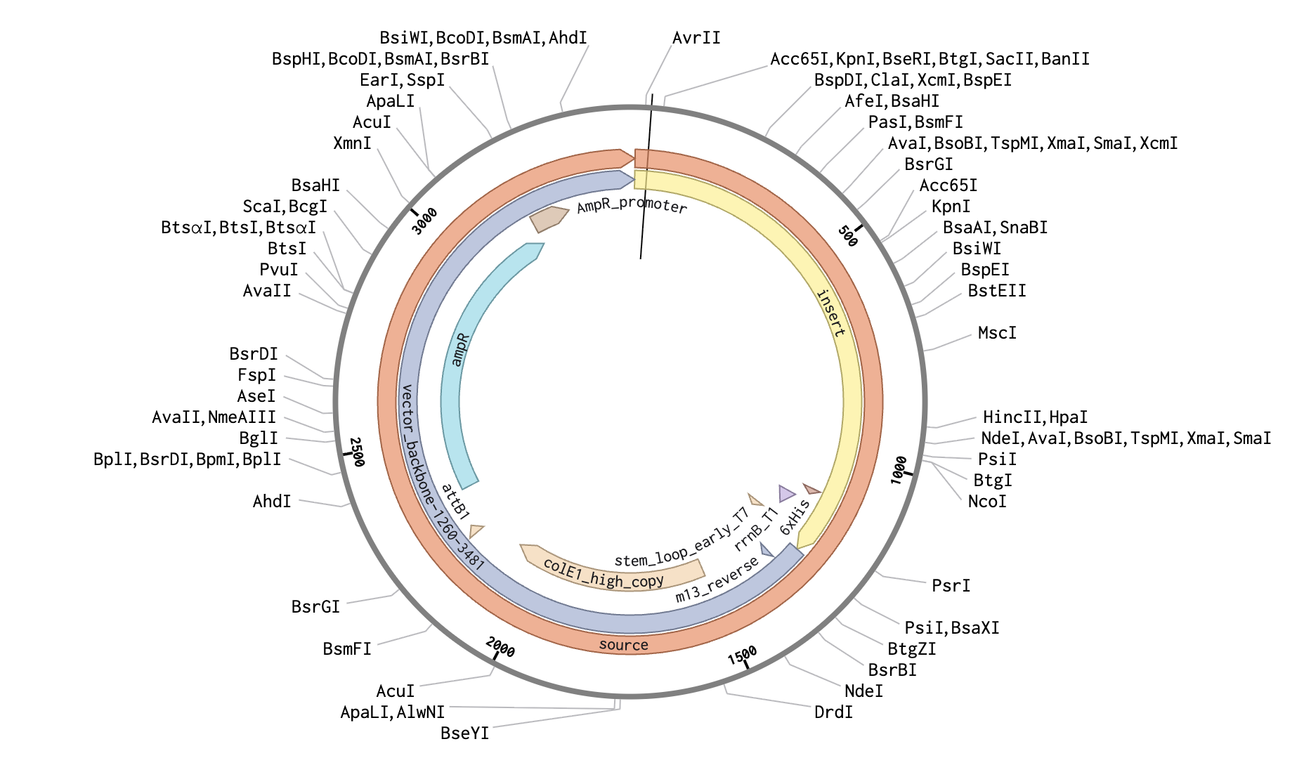
I exported the expression cassette as a FASTA file and uploaded it to Twist as a Clonal Gene using the nucleotide sequence import option. I selected pTwist Amp High Copy as the backbone vector, which provides ampicillin resistance and a high-copy origin of replication. Twist inserts the expression cassette into this backbone to complete the circular plasmid.

I downloaded the full construct as a GenBank file and imported it back into Benchling:

The complete plasmid in Benchling - Reflectin A1 expression cassette inserted into the pTwist Amp High Copy backbone.

DNA Read/Write/Edit

1. DNA Read

What DNA would I want to sequence and why?

I want to sequence DNA that is used for digital data storage — DNA molecules encoding binary information like images, text, or other digital files. The concept is taking digital data (0s and 1s), mapping it onto DNA bases (A, T, G, C), synthesizing those sequences, and storing them physically. DNA is incredibly dense as a storage medium and it lasts without power. George Church’s lab demonstrated this in 2012 by encoding an entire book into DNA.

I am interested in the reading-back problem. Storing data in DNA is only useful if we can reliably retrieve it later, which means sequencing the DNA and decoding it back into the original binary. With the right sequencing technology for retrieval, DNA data storage could become practical for things like archiving cultural heritage, scientific datasets, or even personal data.

What technology would I use?

I would use nanopore sequencing, such as Oxford Nanopore’s MinION device. For DNA data storage, portability matters so that we could read data anywhere outside of just biofacilities.

This is a third-generation sequencing technology: it reads single molecules of DNA directly, without needing to copy the DNA first that rely on PCR amplification which can introduce copying errors.

Input and preparation: The input is the DNA sample containing the encoded data.

1. Library preparation: Attach adapter sequences to the ends of the DNA molecules. They are short DNA sequences with a motor protein attached that guides the strand into the nanopore.
2. No PCR amplification needed: Nanopore sequencing reads native single molecules, so you skip the amplification step that other methods require. This is faster and avoids errors introduced by copying.
3. Load onto the flow cell: Pipette the prepared library onto the MinION flow cell, which contains an array of nanopore proteins embedded in a membrane.

Base calling: Each nanopore is a tiny protein channel in an electrically charged membrane. A voltage drives ionic current through the pore, and when a DNA strand gets fed through by a motor protein, each base (A, T, G, C) blocks the current slightly differently because of its unique size and charge. The device measures these current fluctuations in real time, and a machine learning algorithm figures out the sequence from the pattern of electrical shadow each base casts as it squeezes through a tiny hole.

Output: The outputs are long reads of continuous sequences that can be tens of thousands to millions of bases long and they show up in real time, so we can start seeing results within minutes. For DNA data storage, these reads would be decoded back into binary using whatever encoding scheme was used to write the data.

2. DNA Write

What DNA would I want to synthesize and why?

I want to synthesize a mechanosensitive genetic circuit, a system where living cells can detect physical pressure and produce a visible response. The core component would be MscL (Mechanosensitive Channel of Large Conductance), a protein found in E. coli that acts as a pressure-activated gate in the cell membrane. When the cell experiences mechanical force, MscL opens and allows ions to flow through, which can be wired to trigger gene expression.

The full circuit would involve multiple genes working together: MscL as the sensor, a signal transduction pathway that converts the mechanical input into a transcriptional response, and a fluorescent reporter (like sfGFP) as the visible output. When the cells experience pressure, they glow. What excites me about this is that it’s essentially a biological touch sensor but with living cells instead of electronics. Embedding these cells in a material creates a surface that visually responds to touch.

The DNA I’d need to synthesize would include: the MscL gene (codon-optimized for E. coli), a synthetic promoter responsive to the downstream signal, the sfGFP reporter gene, and the necessary regulatory parts (RBS, terminators).

What technology would I use?

I would use phosphoramidite chemical synthesis, which is the method companies like Twist Bioscience use. This is currently the standard for synthesizing custom DNA sequences.

Essential steps:

1. Sequence design: Design the full multi-gene circuit digitally, codon-optimize for E. coli, and check for synthesis constraints (repeats, GC content, homopolymers).
2. Oligonucleotide synthesis: Short single-stranded DNA fragments (~200 bases) are built one base at a time on a solid support. Each cycle adds one nucleotide through a chemical reaction, with about 99% efficiency per step.
3. Assembly: The short oligos are assembled into longer sequences through overlapping ends.
4. Cloning and verification: The assembled gene is inserted into a plasmid, transformed into E. coli, grown and then sequenced to verify.

Limitations:

• Length: Phosphoramidite chemistry has a practical limit of about 200 bases per oligo because the ~99% per-step yield compounds.
• Repetitive sequences: As I saw with reflectin, repetitive protein motifs create repetitive DNA that is hard to synthesize accurately.
• GC content: Sequences with very high or very low GC content are harder to synthesize because they affect the secondary structure of the DNA during the chemical process.

3. DNA Edit

What DNA would I want to edit and why?

I want to edit the MSTN gene (myostatin) in human muscle cells. Myostatin is a protein that signals muscles to stop growing once they reach a certain size. This makes sense developmentally, but as humans age, muscle mass naturally declines (sarcopenia), leading to frailty, falls, and loss of independence. By editing the myostatin gene, we could preserve muscle mass well into old age.

Myostatin knockouts have been demonstrated across multiple animal species. There are famously muscular “mighty mice” with the gene disabled, and Belgian Blue cattle naturally carry a myostatin mutation that gives them dramatically increased muscle mass. A few humans have been documented with natural myostatin mutations and they show unusually high muscle mass with no apparent negative health effects.

What technology would I use?

I would use CRISPR-Cas9, the most widely used gene editing system. It was adapted from a bacterial immune defense mechanism and has become the standard tool for making precise edits to DNA in living cells. It has two components: the Cas9 protein (molecular scissors that cut DNA) and a guide RNA (a short sequence that tells Cas9 exactly where to cut for gene editing, designed to match the target sequence).

Preparation and steps:

1. Design a guide RNA (~20 nucleotides) matching a region of the MSTN gene, adjacent to a PAM sequence (short DNA motif that Cas9 requires to bind).
2. Assemble the components: Cas9 protein + guide RNA into a ribonucleoprotein complex. RNP delivery is preferred for therapeutic use because it degrades quickly, reducing the risk of unintended edits.
3. Deliver to muscle cells using a viral vector injected into muscle tissue, or lipid nanoparticles.
4. Cas9 cuts the MSTN gene: Once inside the cell, the guide RNA directs Cas9 to the myostatin gene. Cas9 cuts both DNA strands at that spot.
5. Cell repair disrupts the gene: The cell tries to repair the break using a process called non-homologous end joining (NHEJ), which often introduces small insertions or deletions at the cut site which disrupt the gene’s reading frame, effectively no longer producing functional myostatin.

Limitations:

• Off-target edits: The guide RNA might bind to similar sequences elsewhere in the genome and cause unintended cuts.
• Delivery: Getting CRISPR into enough muscle cells across the body is hard. Vectors have limited capacity and can trigger immune responses.
• Mosaic results: Not every cell gets edited, so you end up with a mix of edited and unedited cells. The effect depends on hitting enough of them.
• Irreversibility: Once knocked out, you can’t easily turn the gene back on if something goes wrong.
• Ethical and regulatory concerns: Editing healthy human genomes for enhancement (rather than treating disease) raises significant ethical questions.

Week 3 HW: Lab Automation

Post-Lab Qeustions

1. Paper Review: Automation for Novel Biology

Usai et al. (2023) — “Design and biofabrication of bacterial living materials with robust and multiplexed biosensing capabilities” — Materials Today Bio (open access)

This paper uses a CELLINK INKREDIBLE+ 3D bioprinter, a pneumatic-based, dual-head, computer-controlled extrusion system, to fabricate engineered living materials (ELMs) with spatially arranged bacterial biosensors. The automation principle is similar to the Opentrons where CAD-designed structures are translated into G-code instructions that control precise deposition of biological materials at defined spatial coordinates.

The authors embedded engineered E. coli strains into an alginate/gelatin hydrogel bioink, then used the bioprinter’s dual printheads to deposit different strain-contained bioinks into adjacent separate compartments, creating material structure and biological pattern. Each strain contains a synthetic gene circuit that produces a visible color change (red fluorescent protein) in response to a specific chemical input including quorum sensing molecules (VAI/PAI), IPTG, and tetracycline.

The novel application is the multi-strain spatial logic that automation enables. They built several configurations that would be impossible to fabricate by hand at this precision:

• A level-bar readout — four compartments containing the same VAI sensor but with different promoter strengths (from the Anderson promoter library), so each bar activates at a different chemical concentration threshold which can be used to estimate the analyte concentration range.
• A shuriken-shaped AND gate — 4 compartments each have its own sensing system; one compartment is a boolean logic gate only turns red when both IPTG and VAI are present.
• A cell-cell communication device — two strain types printed in adjacent compartments: a sender strain produces VAI when triggered, and the signal molecule diffuses through the hydrogel to activate a receiver strain (turns red) in an adjacent compartment, creating emergent spatial patterns based on geometry.

The materials were validated in real-world conditions including non-sterile soil, tap water, and clinical bronchial aspirate samples from P. aeruginosa-infected patients, demonstrating that automation-fabricated biosensing materials can function outside the lab. Cell viability persisted over 15 days with periodic subculturing, and the materials remained functional after one month of refrigerated storage.

This paper is directly related to my interest in wearable biosensor arrays using cell-free systems rather than living cells, but the core concept of spatially arranged biosensors that produce colorimetric outputs with built-in signal processing is shared. The automation-enabled precision of multi-compartment spatial arrangement from this paper is inspiring to me.

2. Automation Plan for Final Project

My idea for the final project is to use freeze-dried cell-free (FDCF) reaction spots deposited in a designed spatial array with layered computation capability. When rehydrated, sender spots produce a diffusible signal molecule that travels and activates receiver spots at neighboring positions, producing color. Inspired by the level-bar readout in the paper, receivers contain different concentrations of toehold switch sensor, giving it a different activation threshold. The emergent pattern is non-uniform gradient arising from spatial diffusion distance and engineered sensitivity thresholds.

The emergent pattern depends on three variables: sender/receiver distance, sender concentration, and receiver sensitivity. I intend to use automation in 2 possible ways:

1. Sender/receiver pair screening via Ginkgo Nebula (cloud lab)

Before spatial exploration, I need to identify which cell-free formulations work (individual validation) and which sender/receiver pairs successfully communicate (pair activation). This is suited for cloud lab automation:

1. Echo transfer receiver toehold switch variants + trigger molecules (single validation), and sender reaction outputs + receiver variants (pair screening), into wells
2. Bravo stamp in cell-free TX-TL master mix
3. Multiflo dispense cell-free lysate to start expression
4. PlateLoc seal the plate
5. Inheco incubate at 30–37°C for 1–4 hours
6. XPeel remove seal
7. PHERAstar read colorimetric/fluorescent output

This screens: (a) which receivers produce color when triggered directly, and (b) whether the sender reaction produces enough signal to activate those validated receivers at realistic concentrations.

2. Diffusion-gradient screening via Opentrons OT-2

With validated sender/receiver pairs from Stage 1, I would use the Opentrons to deposit sender and receiver spots to test spatial configurations on my final material (possibly textiles) to find which produce the most compelling emergent patterns. I would need to design a 3D-printed holder for my material to mount on the OT-2 deck.

I used Claude to help understand, develop, and refine this automation plan.

Week 4: Protein Design Part I

Part A: Conceptual Questions

Q1. How many molecules of amino acids do you take with a piece of 500 grams of meat?

500g of meat contains approximately 125g of protein. One mole of a 100-Dalton molecule weighs 100 grams and Avogadro’s number (6.022 × 10²³) is the number of molecules in one mole. So 125g of protein ÷ 100 g/mol = 1.25 moles of amino acid residues, multiplied by Avogadro’s number: 1.25 × 6.022 × 10²³ ≈ 7.5 × 10²³ amino acid molecules.

Q2. Why do humans eat beef but do not become a cow, eat fish but do not become fish?

Digestive enzymes(proteases like pepsin and trypsin) break down the cow’s proteins into individual amino acids via hydrolysis. They are absorbed into our bloodstream and our cells reassemble them into human proteins following the instructions in DNA.

Q3. Why are there only 20 natural amino acids?

The 20 amino acids cover a broad range of chemical properties, positive and negative charges, hydrophobic and hydrophilic, large and small, rigid and flexible structures. This set is chemically diverse enough to build proteins capable of catalyzing thousands of reactions and forming diverse structures. The triplet codon system (64 codons from 4 bases) naturally accommodates around 20 amino acids after accounting for stop codons and redundancy. Early life developed and evolved from this set.

Q5. Where did amino acids come from before enzymes that make them, and before life started?

Amino acids form spontaneously through non-biological chemistry. The Miller-Urey experiment (1953) demonstrated that sparking a mixture of water, methane, ammonia, and hydrogen(simulating early Earth conditions) produced multiple amino acids without any enzymes or cells. Amino acids have also been found on meteorites and detected in interstellar molecular clouds. Energy sources like lightning, UV radiation, and hydrothermal vents can drive the formation of amino acids from simple precursors such as hydrogen cyanide and ammonia. Amino acids are not uniquely biological but are basic organic chemistry that life later organized into a precise system.

Q6. If you make an α-helix using D-amino acids, what handedness (right or left) would you expect?

It would form a left-handed α-helix. Natural L-amino acids produce right-handed α-helices because the L-configuration creates specific steric preferences in backbone angles that favor a right-handed spiral. D-amino acids are the mirror of L-amino acids, so preferences flip and the resulting helix spirals in the opposite direction.

Q7. Can you discover additional helices in proteins?

Yes. Beyond the standard α-helix, other helical forms exist. The 3₁₀ helix is tighter, with hydrogen bonds between amino acid i and i+3 (compared to i and i+4 in the α-helix), making it narrower. The π-helix is wider and looser, with i to i+5 hydrogen bonds. Polyproline helices (type I and II) have no internal hydrogen bonds.

Q8. Why are most molecular helices right-handed?

Life and protein-making exclusively uses L-amino acids, and the L-configuration creates steric preferences that favor right-handed helices. Specifically, in an L-amino acid, the side chain clashes with the backbone carbonyl in a left-handed spiral, which is energetically unfavorable.

Q9. Why do β-sheets tend to aggregate? What is the driving force for β-sheet aggregation?

β-sheets are extended, flat structures with hydrogen bond donors and acceptors exposed along their edges. These unsatisfied hydrogen bonding sites in their edges will bond to those of other β-sheets. This is inherently self-propagating because the outward facing edges drive intermolecular aggregation. The flat faces of stacked β-sheets also interact through hydrophobic packing forces.

Q10. Why do many amyloid diseases form β-sheets? Can you use amyloid β-sheets as materials?

Amyloid diseases involve proteins that misfold into β-sheet-rich structures. The β-sheet conformation is a generic, low-energy state that doesn’t require the precise side-chain packing of a native fold. When a protein misfolds and exposes β-sheet edges, it templates neighboring proteins to misfold the same way, creating a self-propagating cascade. Amyloid β-sheets can be used as materials because they have tensile strength comparable to steel, resist heat and proteases, and self-assemble spontaneously. Researchers have used them as scaffolds for tissue engineering, conductive nanowires, adhesive coatings, and hydrogel matrices for cell culture.

Part B: Protein Analysis and Visualization

Protein Selection

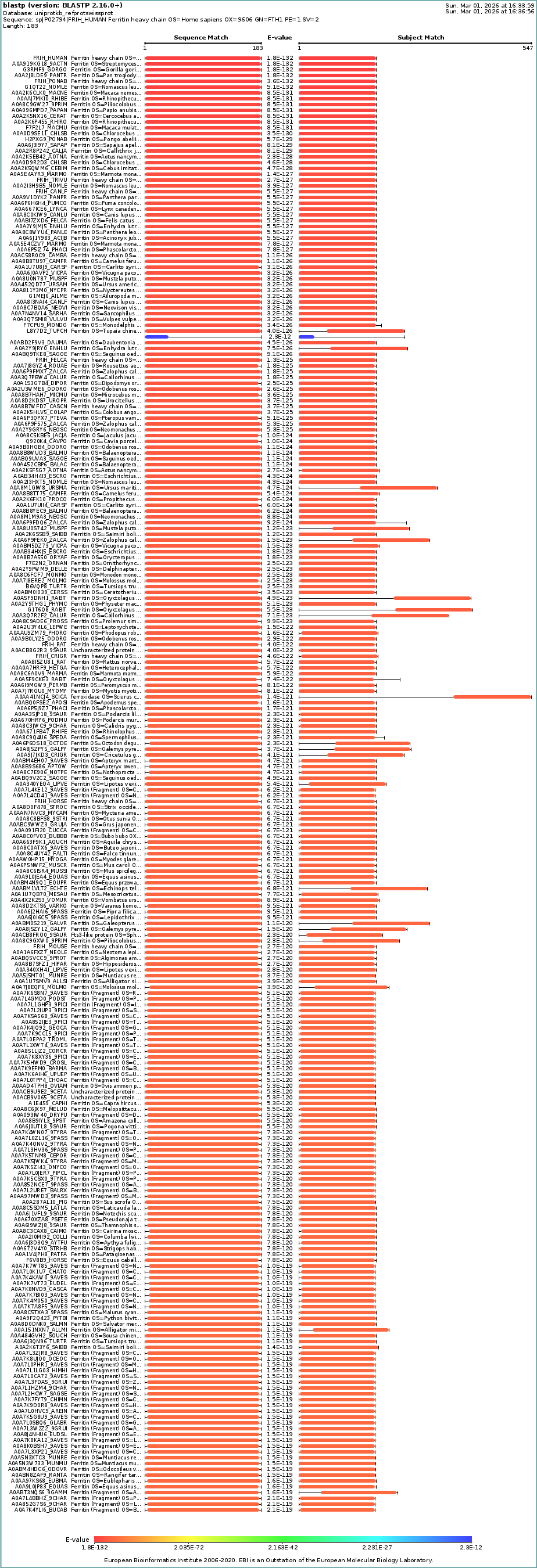
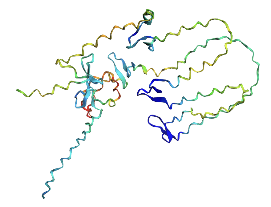
I selected human heavy-chain ferritin (HuHF), the primary iron-storage protein found in virtually all living organisms. I chose this because its self-assembling architecture makes it a powerful platform for nanotechnology applications including drug delivery, biosensor scaffolding, and templated nanomaterial synthesis. Ferritin represents a natural example of the design principle: simple modular subunits that autonomously organize into functional nanostructures.

Sequence Analysis

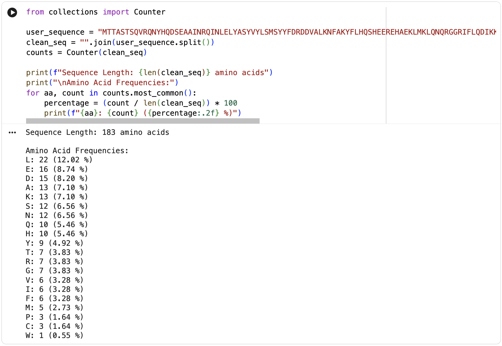
The protein is 183 amino acids long. The most frequent amino acid is leucine (L).

Homologs: BLAST search of UniProt identified at least 250 homologs at ≥90% sequence identity, including primates, other mammals, and even bacteria.

Protein Family: Ferritin belongs to the ferritin-like superfamily (Pfam: PF00210). This superfamily also includes bacterioferritins and DNA-binding proteins from starved cells (Dps proteins). InterPro classifies it under the ferritin/ribonucleotide reductase-like domain family.

RCSB Structure

Protein Structure on RCSB: https://doi.org/10.2210/pdb1FHA/pdb

When was it solved: deposited in 1990 and released in 1992, with the primary citation published in 1991 (Lawson et al., Nature 349: 541-544). It was solved by X-ray crystallography at a resolution of 2.40 Å(good quality). The R-value of 0.205 further confirms the model fits the experimental data well.

Other molecules in the structure: The structure contains two types of non-protein molecules: iron (Fe³⁺) ions located at the ferroxidase center within each of its four-helix bundle, which is where ferritin catalyzes the oxidation of Fe²⁺ to Fe³⁺ for storage; and calcium (Ca²⁺) ions, likely present from crystallization conditions.

Structure classification: The protein is classified as a METAL BINDING PROTEIN with the enzyme classification EC 1.16.3.1 (ferroxidase). The biological assembly has octahedral symmetry (O) as a homo 24-mer (A24), with each subunit folded as a four-helix bundle.

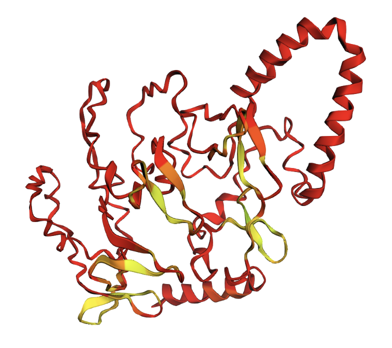
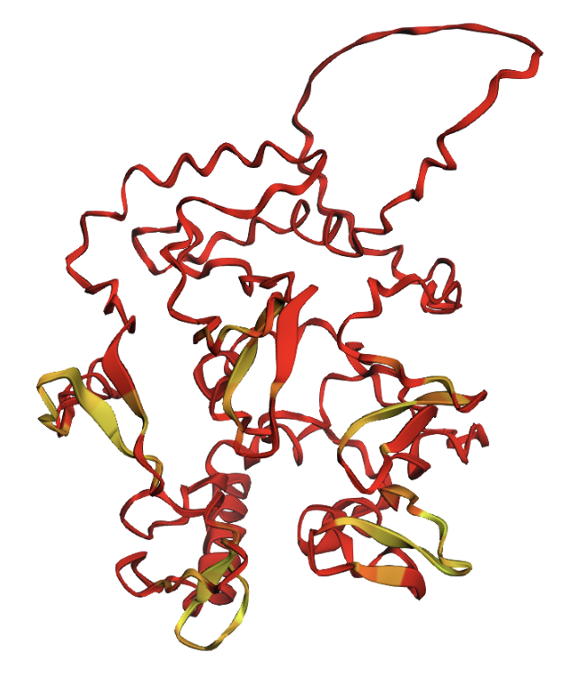
PyMOL Visualization

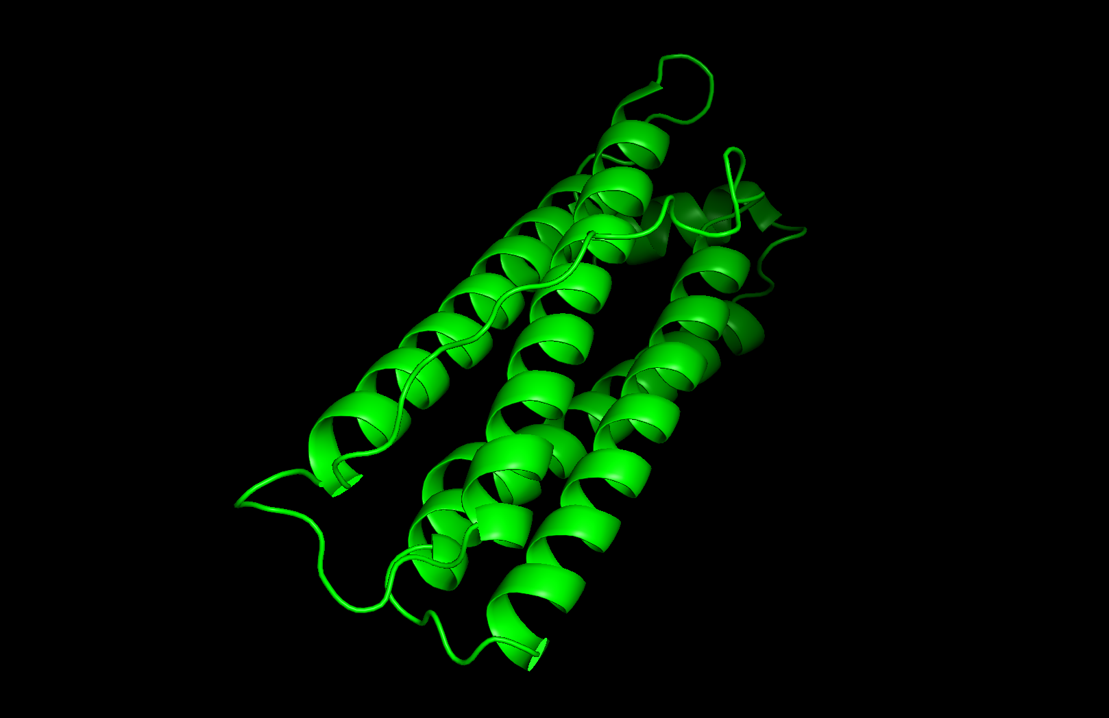
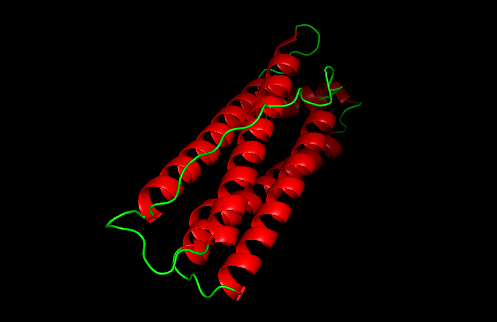
Cartoon visualization

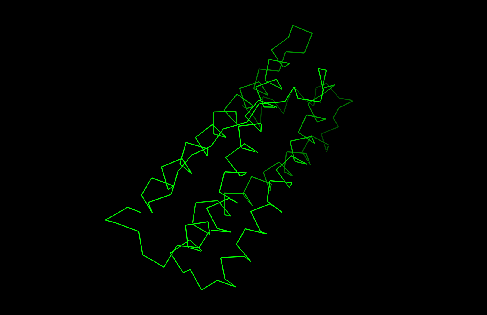
Ribbon visualization

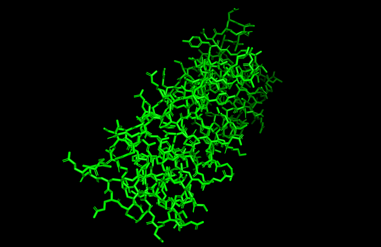
Ball and stick visualization

Secondary structure: The protein is almost entirely alpha-helical (red) with no beta-sheets. The only non-helical regions (green) are short loops connecting the four main helices.

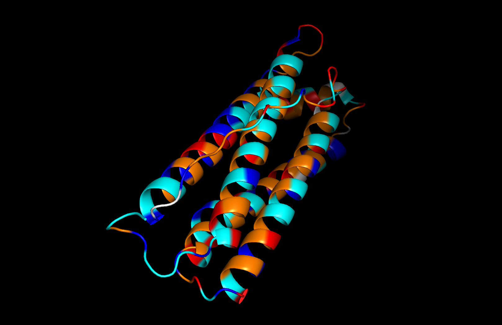
Residue type: Hydrophobic residues (orange) and hydrophilic/charged residues (cyan, blue, red) are interspersed along the helices, but the hydrophobic residues face inward toward the bundle core while charged and polar residues face outward toward solvent. This inside-out arrangement is typical of soluble proteins.

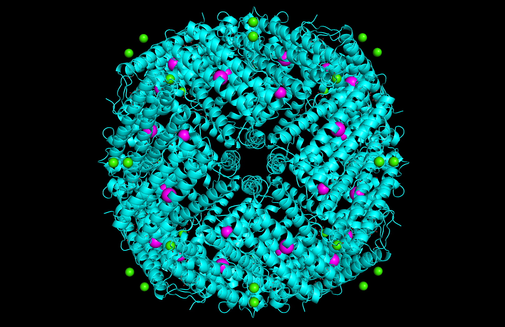
Surface and binding pockets: The 24-mer assembly reveals a hollow spherical cage with visible pores which are the channels through which iron ions enter and exit the interior cavity. Iron atoms (magenta spheres) are visible at the ferroxidase centers within each subunit, and calcium ions (green spheres) sit at the symmetry axes.

Part C: Using ML-Based Protein Design Tools

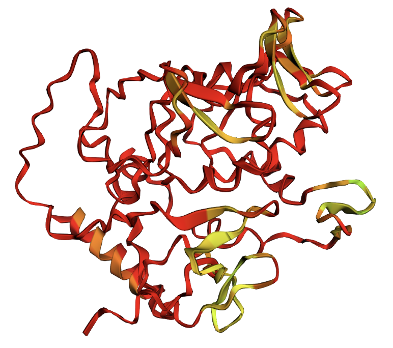
For Part C, I chose Reflectin A1 from Doryteuthis pealeii (longfin inshore squid), the protein responsible for dynamic structural coloration in cephalopod skin.

C1. Protein Language Modeling

Deep Mutational Scan

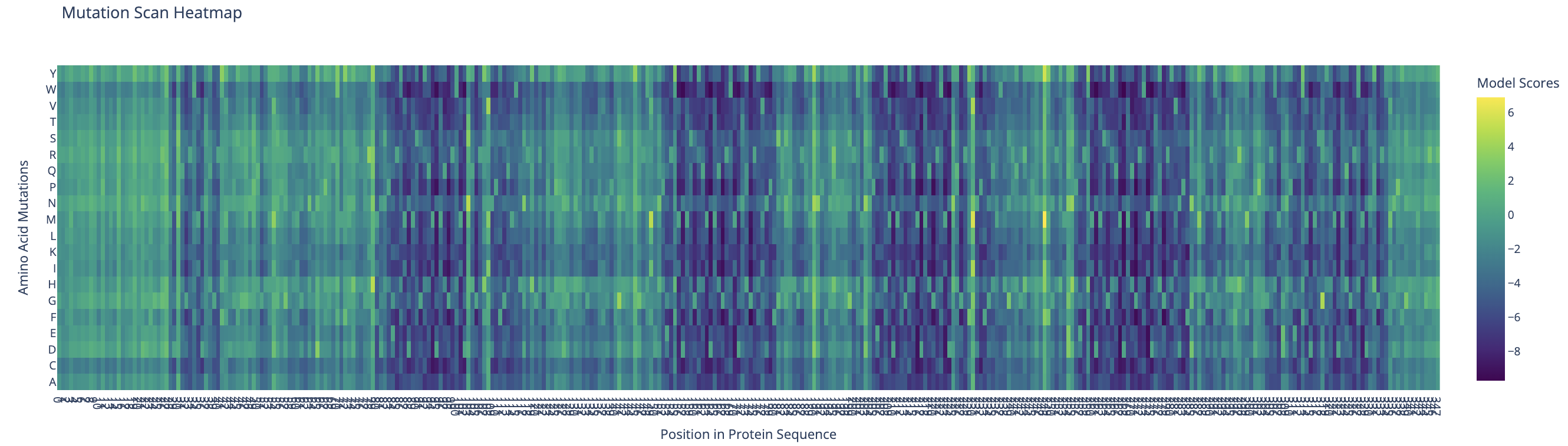
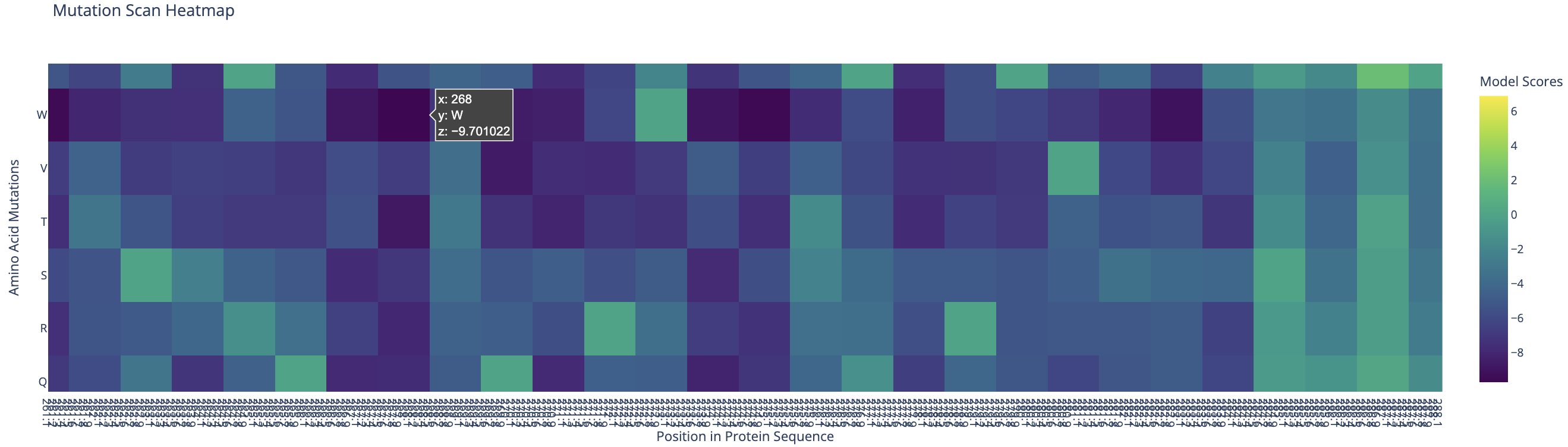
I used ESM-2 to perform the deep mutational scan of Reflectin A1 (350 aa) in RELATIVE mode, scoring the predicted effect of every possible single amino acid substitution at every position.

ESM-2 deep mutational scan heatmap. X-axis: position in sequence (1–350). Y-axis: amino acid substitutions. Color: model score (yellow = tolerated, dark blue/purple = deleterious).

The heatmap reveals regularly spaced clusters of mutation-intolerant positions approximately every 50–70 residues. This periodicity suggests the model has learned the repeating internal motif structure of the reflectin family. Cysteine(C) and tryptophan(W) substitutions are the most strongly penalized across these positions, likely because introducing disulfide-forming or large aromatic residues at these sites would disrupt the native fold.

Standout residue: Position 268 mutated to tryptophan (W) scored −9.70, the most deleterious prediction in the scan. It is also intolerant to methionine, leucine, lysine, and isoleucine, which suggests the original residue at this position is structurally or functionally critical and cannot be replaced without disrupting the protein.

Latent Space Analysis

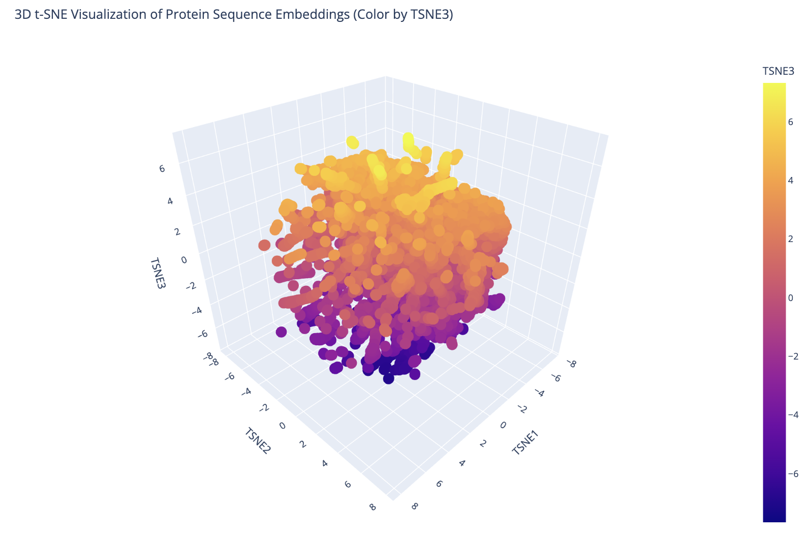
I embedded 15,177 proteins from the ASTRAL SCOP structural classification database using ESM-2 mean token embeddings (320 dimensions), then reduced them to 3D with t-SNE for visualization. The resulting plot shows clear clustering — proteins with similar sequences and structures group into distinct neighborhoods, confirming that ESM-2’s learned representations capture meaningful structural relationships.

3D t-SNE visualization of 15,177 ASTRAL SCOP protein embeddings colored by TSNE3 component. Distinct clusters correspond to different protein fold families.

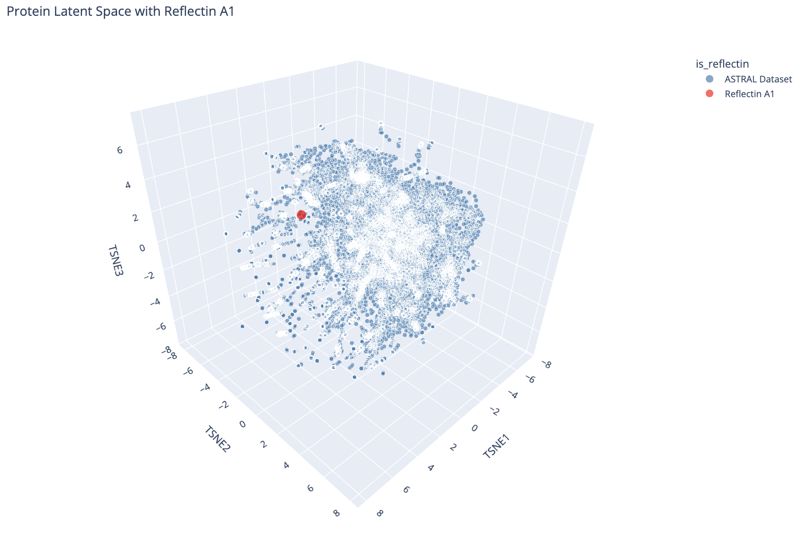
I then embedded Reflectin A1 into the same space and projected it alongside the ASTRAL dataset.

Reflectin A1 (red dot) plotted in the ESM-2 latent space alongside the ASTRAL dataset (blue). It sits near the periphery of the main cluster.

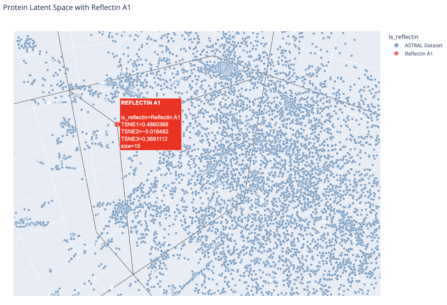
Zoomed view showing Reflectin A1’s position relative to nearby ASTRAL proteins.

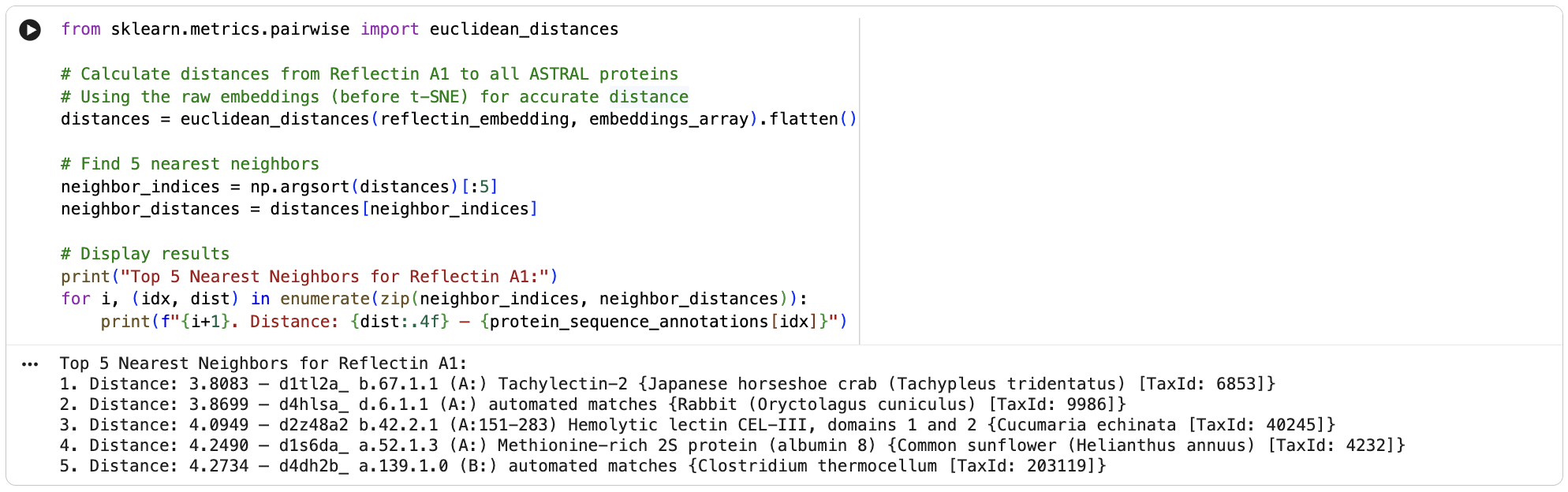
Using Euclidean distance in the original 320-dimensional embedding space, the 5 nearest neighbors to Reflectin A1 are:

1. Tachylectin-2, Japanese horseshoe crab (dist: 3.81)
2. Rabbit protein, automated match (dist: 3.87)
3. Hemolytic lectin CEL-III, sea cucumber (dist: 4.09)
4. Methionine-rich 2S albumin, sunflower (dist: 4.25)
5. Clostridium thermocellum protein, automated match (dist: 4.27)

Two of the five closest neighbors are lectins with repetitive structural motifs used for carbohydrate binding. Reflectin also contains repetitive internal motifs, so ESM-2 may be picking up on this shared repetitive sequence character despite the proteins being functionally unrelated. The methionine-rich neighbor is also notable since reflectin is unusually rich in methionine. The relatively large distances across all five neighbors (3.8–4.3) confirm that reflectin has no close structural homologs in the database, consistent with it being a structurally novel protein unique to cephalopods.

C2. Protein Folding

Folding with ESMFold

I folded Reflectin A1 using ESMFold and compared the result to the AlphaFold prediction.

ESMFold produced very low confidence scores: a pLDDT of 39.15 (out of 100) and pTM of 0.157 (out of 1). Values below 50 pLDDT indicate intrinsic disorder. The structure is almost entirely red when colored by confidence, meaning ESMFold cannot confidently predict any region of the fold.

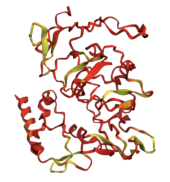
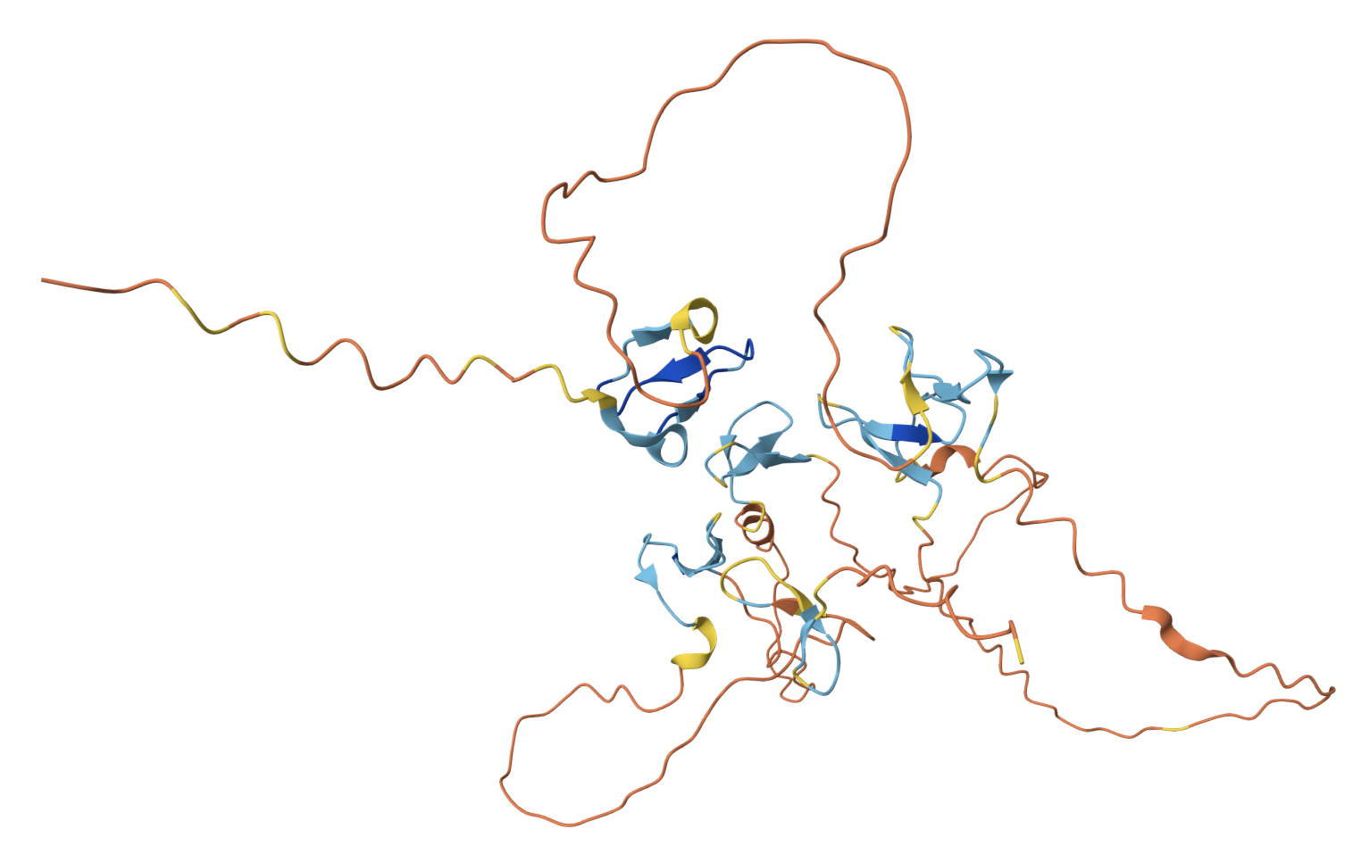
ESMFold prediction colored by pLDDT confidence. Red = very low confidence, yellow = slightly higher confidence. The protein is almost entirely red.

AlphaFold prediction for comparison. Both models show the protein is largely disordered, but AlphaFold identifies a few small β-sheet domains (blue) within the repetitive regions that ESMFold misses entirely.

Mutation Resilience

I tested whether the predicted structure is sensitive to mutations by single substitutions and large segment replacements:

Q268W single mutation: virtually identical to original.

W81A single mutation: virtually identical to original.

Positions 100–130 replaced with all alanines. A helix appears in the alanine region, but confidence remains low.

Positions 200–230 replaced with all glycines. A large disordered loop appears where the glycines were inserted.

Single mutations had essentially no effect on the predicted structure where pTM remained identical at 0.157 and pLDDT changed by less than 0.5 points. Even replacing 31 consecutive residues with alanines or glycines only reduced pLDDT by 0.5–2.7 points. The glycine segment had the largest effect (pLDDT dropped from 39.15 to 36.48), likely because glycine is the most flexible residue and further destabilized an already disordered region. The structure appears highly resilient to mutation because there is so little predicted structure to begin with. ESMFold already has near-zero confidence in the original sequence, so mutations cannot meaningfully change much.

C3. Protein Generation (Inverse Folding)

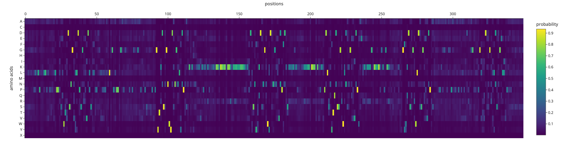
I used ProteinMPNN (v_48_020, sampling temperature 0.1) to perform inverse folding on the AlphaFold-predicted backbone of Reflectin A1.

ProteinMPNN amino acid probabilities at each position. Bright spots indicate positions where the model is highly confident about which residue should occupy that position.

The designed sequence had a sequence recovery of only 16.9%, meaning ProteinMPNN’s ideal sequence for this backbone is extremely different to the actual reflectin sequence. Reflectin sequence is optimized for self-assembly and dynamic nanostructure formation by sticking to other reflectin molecules. Many reflectin proteins come together and stack into organized layers, and it’s those layers that create the structural color (iridescence) in squid skin. The spacing between layers determines what wavelength of light gets reflected. ProteinMPNN designs for structural stability rather than the intermolecular interactions.

Folding the Designed Sequence with ESMFold

I folded the ProteinMPNN-designed sequence with ESMFold to compare it to the original:

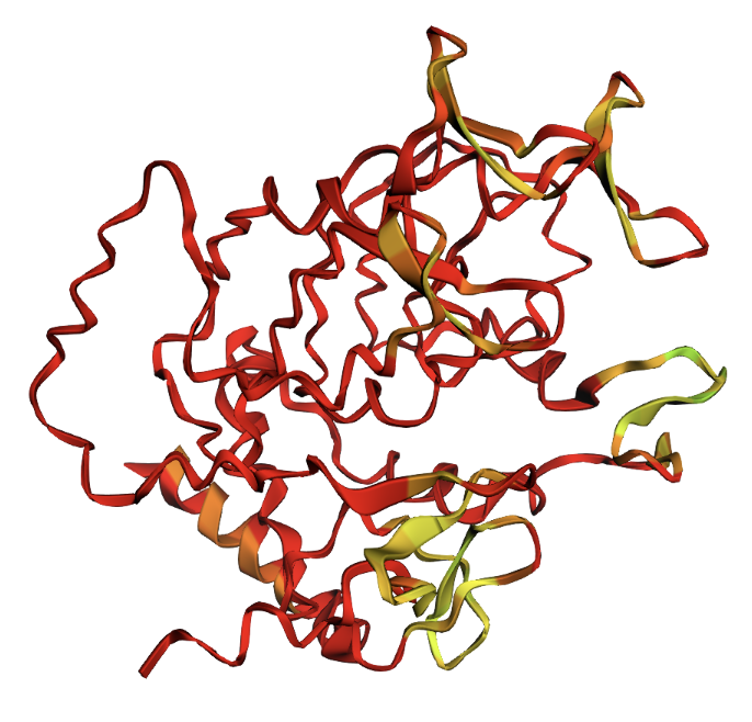
ESMFold prediction of the ProteinMPNN-designed sequence. The structure shows substantially more secondary structure elements (helices and sheets) compared to the original.

The ProteinMPNN-designed sequence folds with dramatically higher confidence (pLDDT 72.86 vs 39.15). The designed sequence contains many more prolines, glycines, and lysines residues that promote stable secondary structures and far fewer of reflectin’s characteristic methionine-rich and aromatic motifs. This highlights a fundamental tension in protein engineering: a sequence that folds well as a monomer is not necessarily a sequence that functions correctly.

Week 5: Protein Design Part II

Part A: SOD1 Binder Peptide Design

Design of short peptides targeting the A4V mutant of human SOD1 (P00441) as a potential therapeutic strategy for familial ALS.

Part 1: Generate Binders with PepMLM

SOD1 Original Sequence:

A4V Mutant SOD1 Sequence

Binder Results

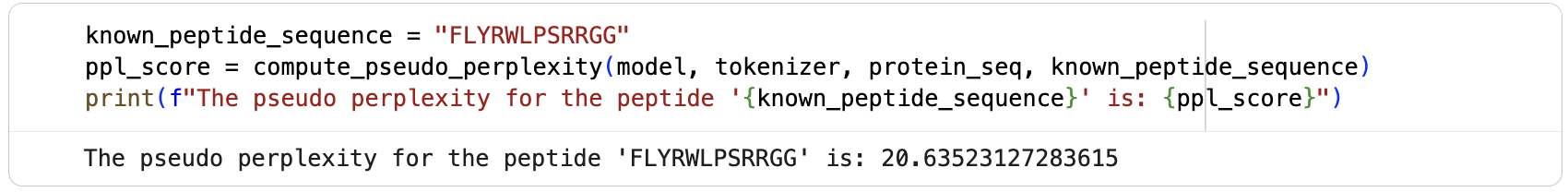
Four 12-mer peptides were generated by PepMLM-650M, and the known SOD1-binding peptide FLYRWLPSRRGG was scored separately for comparison.

Part 2: Evaluate Binders with AlphaFold3

Each peptide was co-folded with the A4V mutant SOD1 sequence as separate chains using the AlphaFold3 server. Peptide 4 (WHYYVAGLEHKX) could not be submitted due to the ambiguous X residue.

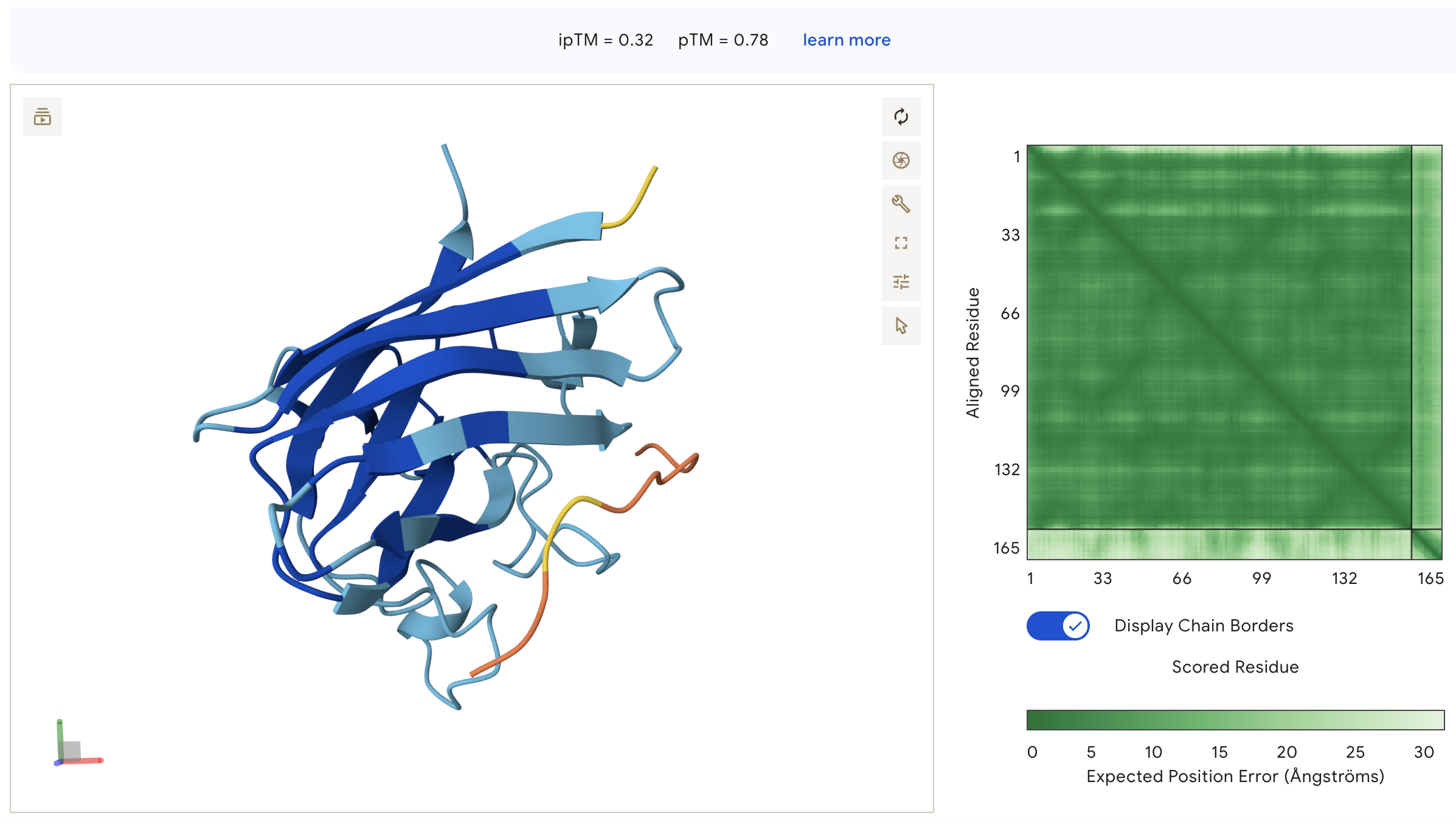
Peptide 1: WHYYAVVARHKE (ipTM = 0.32)

WHYYAVVARHKE: ipTM = 0.32, peptide appears as an unstructured surface-bound loop that is not contacting the N-terminus where A4V sits, with high inter-chain PAE indicating poorly defined binding.

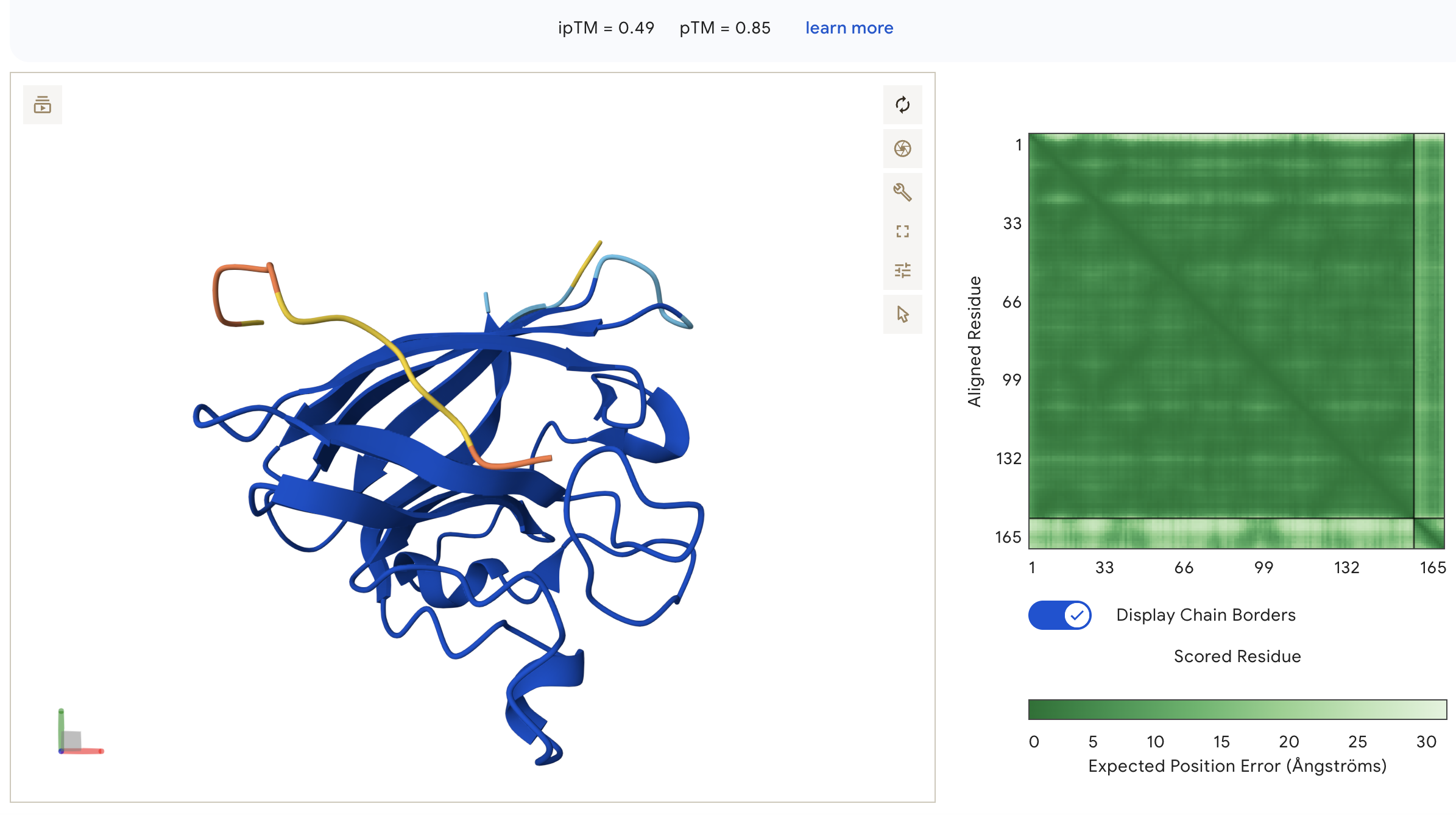
Peptide 2: WRVGAVGVAHKK (ipTM = 0.49)

WRVGAVGVAHKK: ipTM = 0.49, peptide appears as an unstructured loop on the opposite face from the N-terminus, with high inter-chain PAE indicating poorly defined binding, though ipTM is notably higher than all other peptides including the known binder.

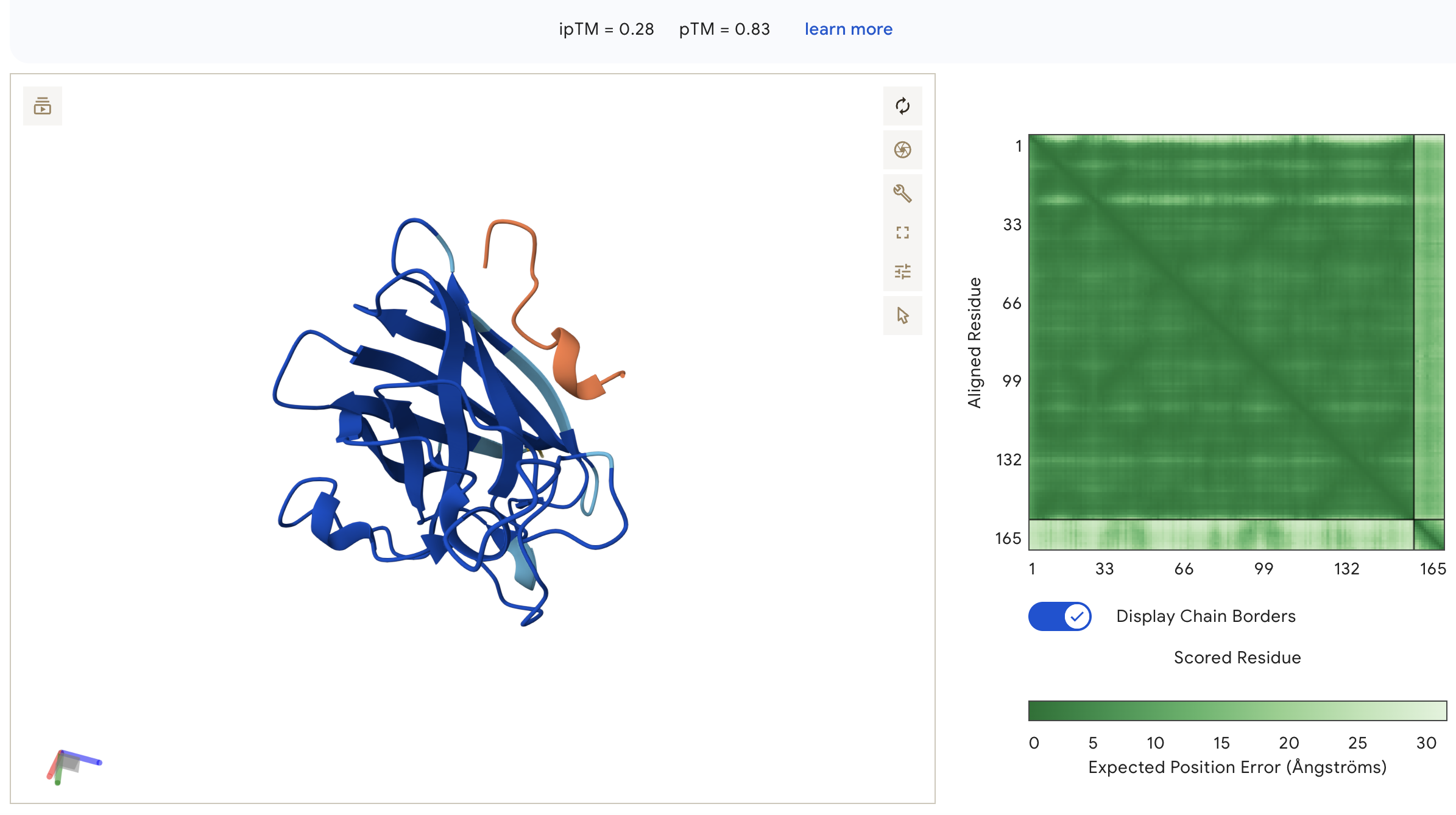
Peptide 3: WHSYATVVEHWE (ipTM = 0.28)

WHSYATVVEHWE: ipTM = 0.28, peptide is surface-bound on the lateral face of the β-barrel away from the N-terminus, with very light inter-chain PAE indicating the weakest binding confidence of all peptides.

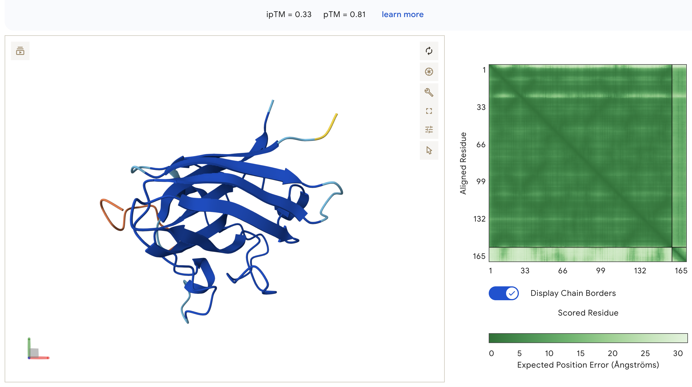
Known Binder: FLYRWLPSRRGG (ipTM = 0.33)

FLYRWLPSRRGG: ipTM = 0.33, peptide wraps around the lateral face of the β-barrel as an extended unstructured loop, with no engagement near the N-terminus and high inter-chain PAE indicating poorly defined binding geometry.

All peptides scored below 0.5 ipTM, indicating low overall interface confidence across the set; however, peptide 2 (WRVGAVGVAHKK) achieved the highest ipTM at 0.49, exceeding the known binder (0.33), suggesting it is the strongest structural candidate despite none localizing clearly to the N-terminal A4V site.

Part 3: Evaluate Properties with PeptiVerse

Each peptide was evaluated against the A4V mutant SOD1 sequence using PeptiVerse for predicted binding affinity, solubility, hemolysis probability, net charge, and molecular weight.

Peptide 1: WHYYAVVARHKE

Peptide 2: WRVGAVGVAHKK

Peptide 3: WHSYATVVEHWE

Known Binder: FLYRWLPSRRGG

Higher ipTM does not correlate with stronger predicted binding affinity; peptide 3 (WHSYATVVEHWE) shows the highest affinity (5.604) despite the lowest ipTM (0.28), while peptide 2 (WRVGAVGVAHKK) has the best structural confidence but mid-range affinity (5.520); all peptides are predicted soluble and non-hemolytic, making peptide 2 the best overall candidate as it balances the strongest structural binding (ipTM 0.49), low hemolysis risk (0.020), and relatively good binding affinity.

Part 4: Motif-Guided Generation with moPPIt

moPPIt was run targeting motif positions 1–8 of A4V SOD1, with objectives set to Hemolysis, Solubility, Affinity, and Motif (all weights = 1). Four 12-mer peptides were generated.

Comparison and Evaluation

PepMLM peptides are dominated by aromatic residues (W, H, Y, F), while moPPIt peptides are more compositionally diverse featuring charged and polar residues alongside three cysteine-containing sequences because generation was guided by multiple objectives. The moPPIt set achieves higher predicted affinity overall, though motif adherence varies: EKASGGHEHNPI scores only 0.364. The computational scores are predictions, not measurements so the first step is to actually test whether these peptides bind A4V SOD1 in the lab and confirm the predicted properties hold experimentally. From there, you would test whether binding has a functional effect in cells and what type of delivery method.

Part C: L-Protein Mutant Design

The MS2 lysis protein (UniProt P03609) is a 75-residue protein with a soluble N-terminal domain (residues 1–40) that interacts with the E. coli chaperone DnaJ, and a transmembrane domain (residues 41–75) responsible for membrane poration and lysis. The goal is to engineer mutants that improve DnaJ-independence or lysis efficiency to overcome bacterial resistance.

Mutation Selection

Five mutants were selected using three sources: (1) experimental lysis data from Chamakura et al., (2) ESM-2 log-likelihood ratio (LLR) scores from the Colab notebook, and (3) conservation analysis across 26 homologous sequences from pBLAST.

Mutations were selected where experimental data confirmed both Lysis=1 and Protein Levels=1, meaning the mutant phage still kills bacteria and still produces the protein. Conserved positions with strong experimental support were also included.

The ESM-2 LLR scores weakly correlate with the experimental lysis data. S15A and A45P have near-zero LLR scores (tolerated but not predicted as beneficial), while R18G, R30Q, and L44P are all negative where the model predicts these as slightly harmful. Yet all five maintain lysis experimentally.

S15A: position 15 is variable across MS2 strains, and A is observed in nature at this position, making this the most conservative and well-supported mutation. Located in the soluble domain, it may alter DnaJ interaction.

R18G and R30Q: both in the soluble domain at conserved positions, but directly confirmed by experimental data to maintain lysis function.

L44P and A45P: in the transmembrane domain. Both are experimentally confirmed to maintain lysis (Lysis=1, Protein=1) with only A45P variable in nature.

Week 6: Genetic Circuit Part I

DNA Assembly

Q1. What are some components in the Phusion High-Fidelity PCR Master Mix and what is their purpose?

Phusion Master Mix contains Phusion DNA Polymerase, which has 3’ to 5’ proofreading exonuclease activity that corrects misincorporated bases, with a much lower error rate than standard Taq polymerase. dNTPs are the substrate for new strand synthesis. A reaction buffer maintains optimal pH and ionic conditions, and includes MgCl₂ as a required cofactor for polymerase function and primer binding.

Q2. What are some factors that determine primer annealing temperature during PCR?

Annealing temperature is primarily set by the primer melting temperature. Longer primers have a higher melting temperature because more base pairs stabilize binding. Higher GC content raises the temperature because GC pairs form three hydrogen bonds versus two for AT pairs, which requires more energy to break.

Q3. Compare and contrast PCR and restriction enzyme digests.

PCR makes copies of a DNA fragment, and works on any sequence because the primers are designed to control what the ends of the fragment look like. Custom overhang sequences make PCR useful for Gibson assembly. The downside is that polymerase can occasionally introduce errors, and very long fragments are hard to amplify.

Restriction enzymes simply cut DNA at specific recognition sequences to produce fragments with defined sticky or blunt ends which cannot be customized. They do not copy DNA or introduce mutations. It is simpler and error-free but requires the right recognition sites to already be present in the sequence.

PCR is better when generating a fragment from scratch or needing custom ends for cloning. Restriction digestion is preferred when vectors already have the mapped restriction cut sites.

Q4. How can you ensure that the DNA sequences that you have digested and PCR-ed will be appropriate for Gibson cloning?

First, primers must be designed with approximately 20 or more base pairs of overlapping sequence between adjacent fragments so the Gibson enzymes can recognize and join them. Second, fragment sizes should be confirmed by gel electrophoresis. Third, PCR products must be purified using a column cleanup kit to remove leftover primers, polymerase, and salts that would interfere with the assembly reaction.

Q5. How does the plasmid DNA enter the E. coli cells during transformation?

In heat shock transformation, cells are treated with cold CaCl₂ to make them competent, then briefly heated to 42°C for 45 seconds. This thermal shock disrupts the membrane, allowing plasmid DNA to enter. The cells are then rapidly cooled on ice to close the pores. Cells then recover in SOC media before plating on an agar plate.

Q6. Describe another assembly method in detail.

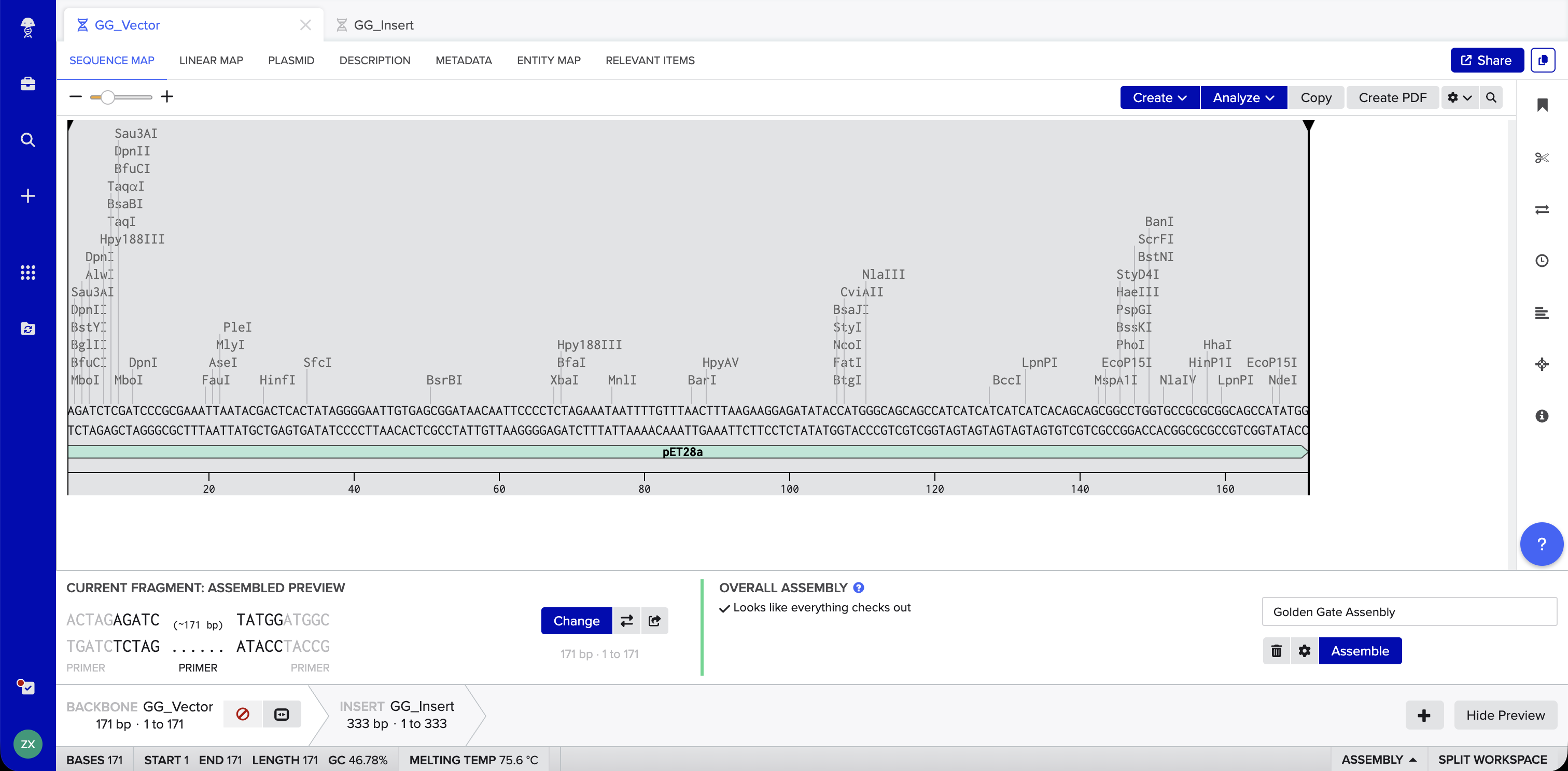
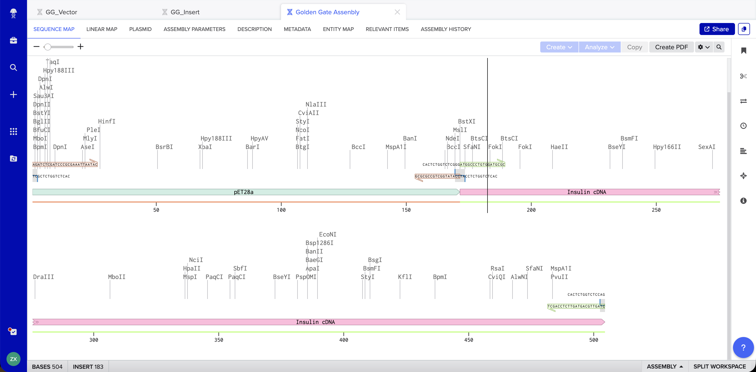
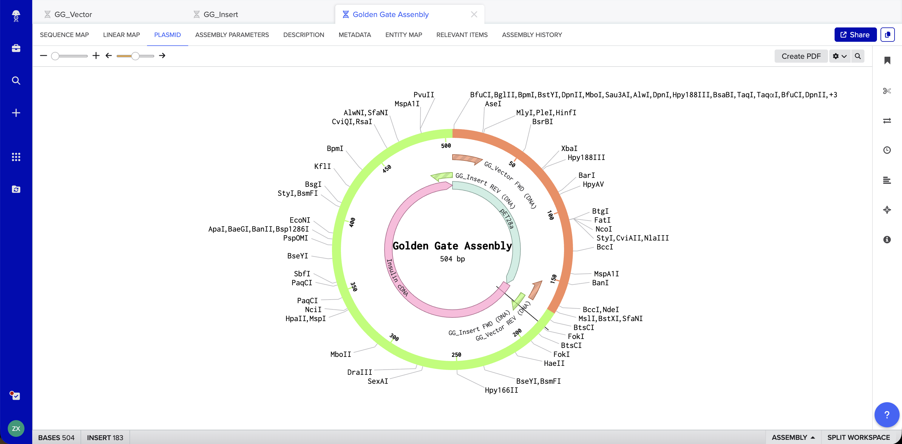
Golden Gate Assembly uses Type IIS restriction enzymes (such as BsaI) to generate unique 4-bp sticky ends on each DNA fragment. Unlike standard restriction enzymes, Type IIS enzymes cut outside their recognition sequence, so the recognition site is absent from the final product. Each junction is designed with a unique overhang, ensuring fragments can only assemble in one correct order. The reaction runs with both restriction enzyme and ligase in a single tube, cycling between digestion and ligation temperatures until the correct assembly accumulates.

Benchling Simulation: The assembly was modeled in Benchling using a pET28a-derived vector (GG_Vector), a widely used bacterial expression vector, as the backbone and an insulin cDNA insert (GG_Insert). Benchling automatically designed four primers with BsaI recognition sites and generated sticky ends GGAT and AGAG at the two junctions. The plasmid map shows the vector and insert joined into a 504 bp circular construct with 0 errors and 0 warnings.

Asimov Kernel

Repository: Annie_Week 6 HW

Repressilator

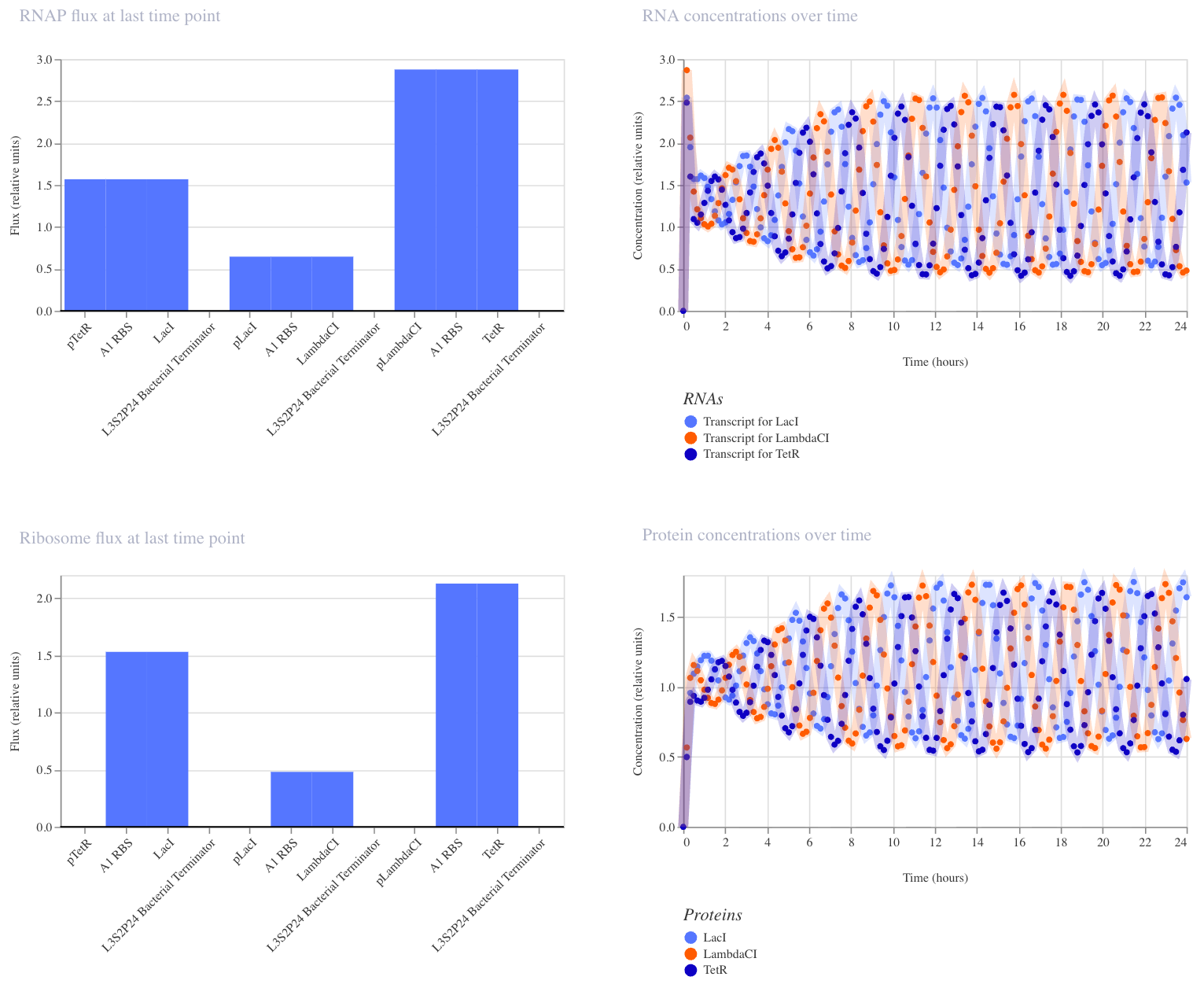
The repressilator is a synthetic genetic oscillator where three repressors are arranged in a negative feedback loop; each repressor inhibits the promoter driving the next:

pTetR → LacI → pLacI → LambdaCI → pLambdaCI → TetR → (back to pTetR)

No single protein can stay high for long, so the system continuously oscillates. I recreated the circuit in Kernel using parts from the Characterized Bacterial Parts repository and ran the simulator (E. coli, 24 hours, 10-minute timestep, transient transfection, no ligands). The simulator shows the expected oscillating expression of three repressor proteins (LacI, LambdaCI, TetR) cycling out of phase over 24 hours, confirming that each protein suppresses the next in the loop.

Custom Constructs

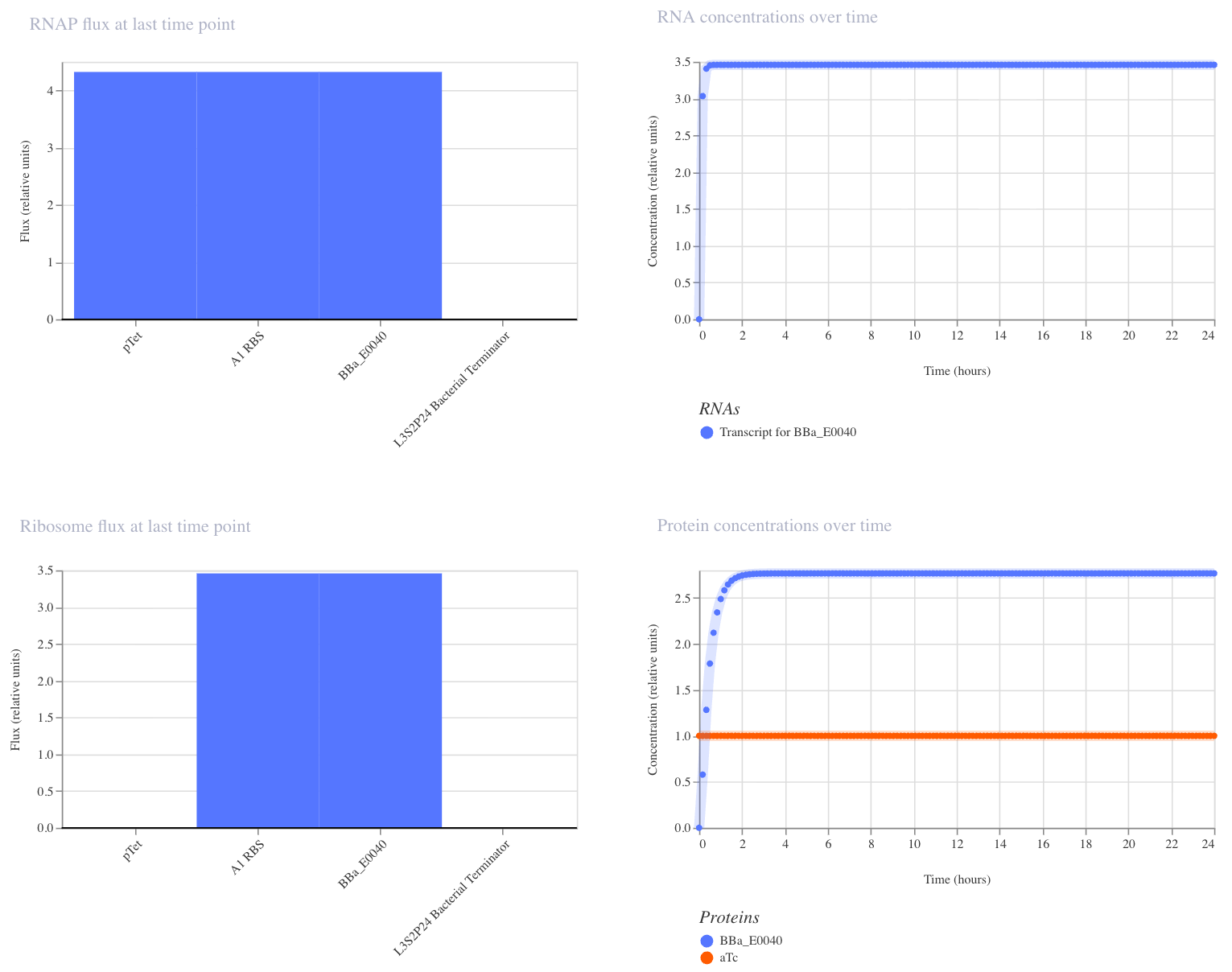
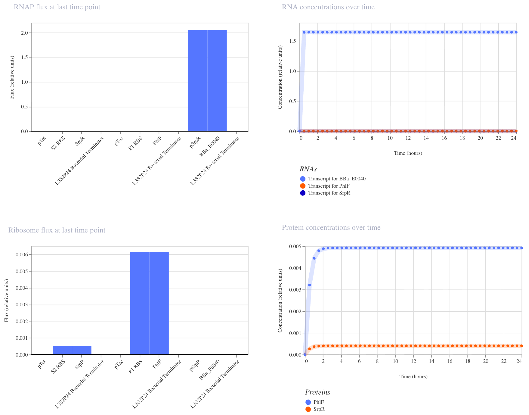
1. Single Reporter

This construct is a simple on/off switch: a single promoter (pTet) drives expression of GFP (BBa_E0040). pTet is normally repressed, but when aTc is added, it blocks that repression and GFP is produced. GFP should rise and hold steady after aTc addition.

I ran the simulator with aTc added at hour 0 (E. coli, 24 hours, 10-minute timestep, transient transfection). GFP rose quickly and plateaued at ~2.7 relative units, confirming that the circuit switches on as expected.

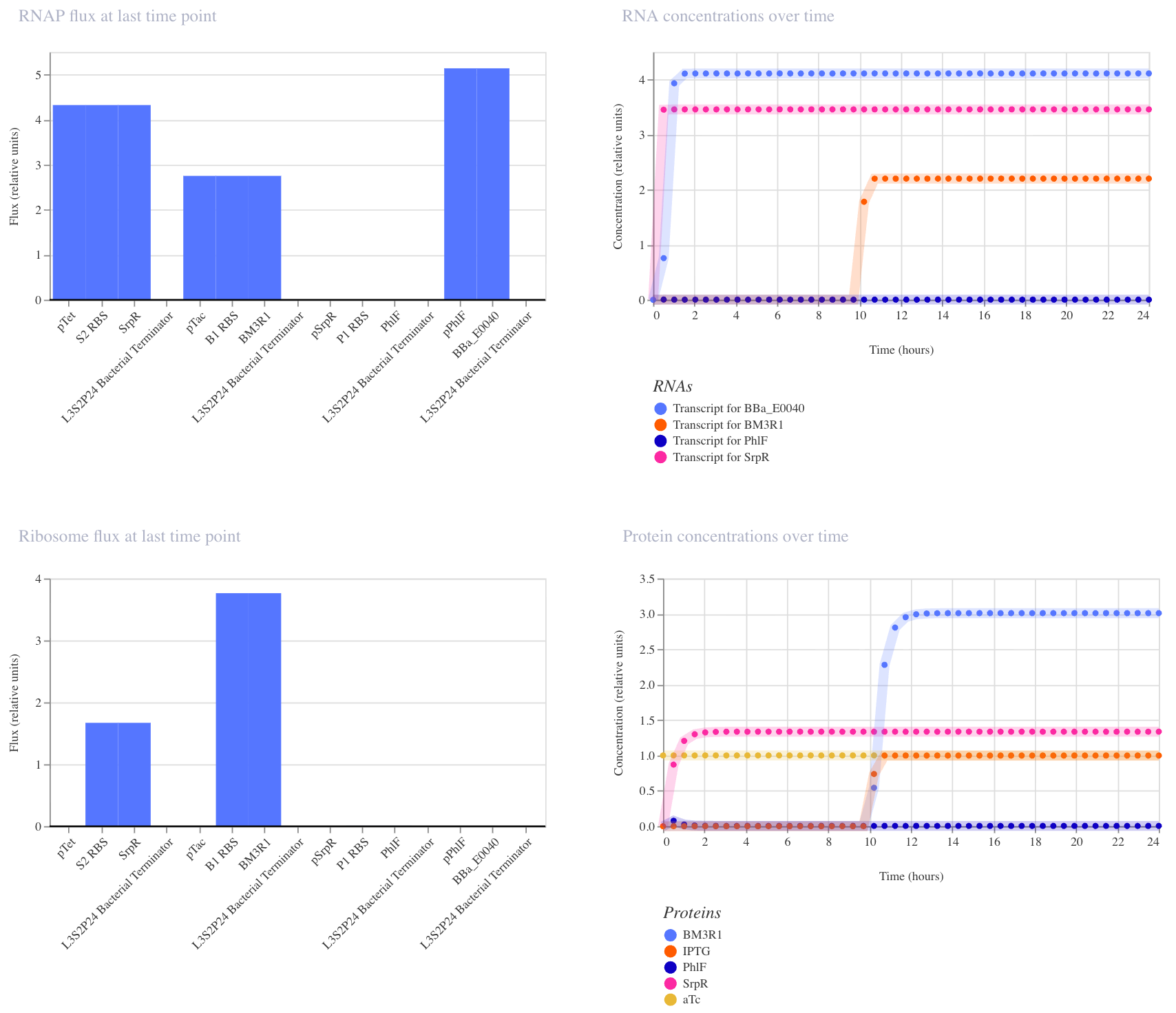
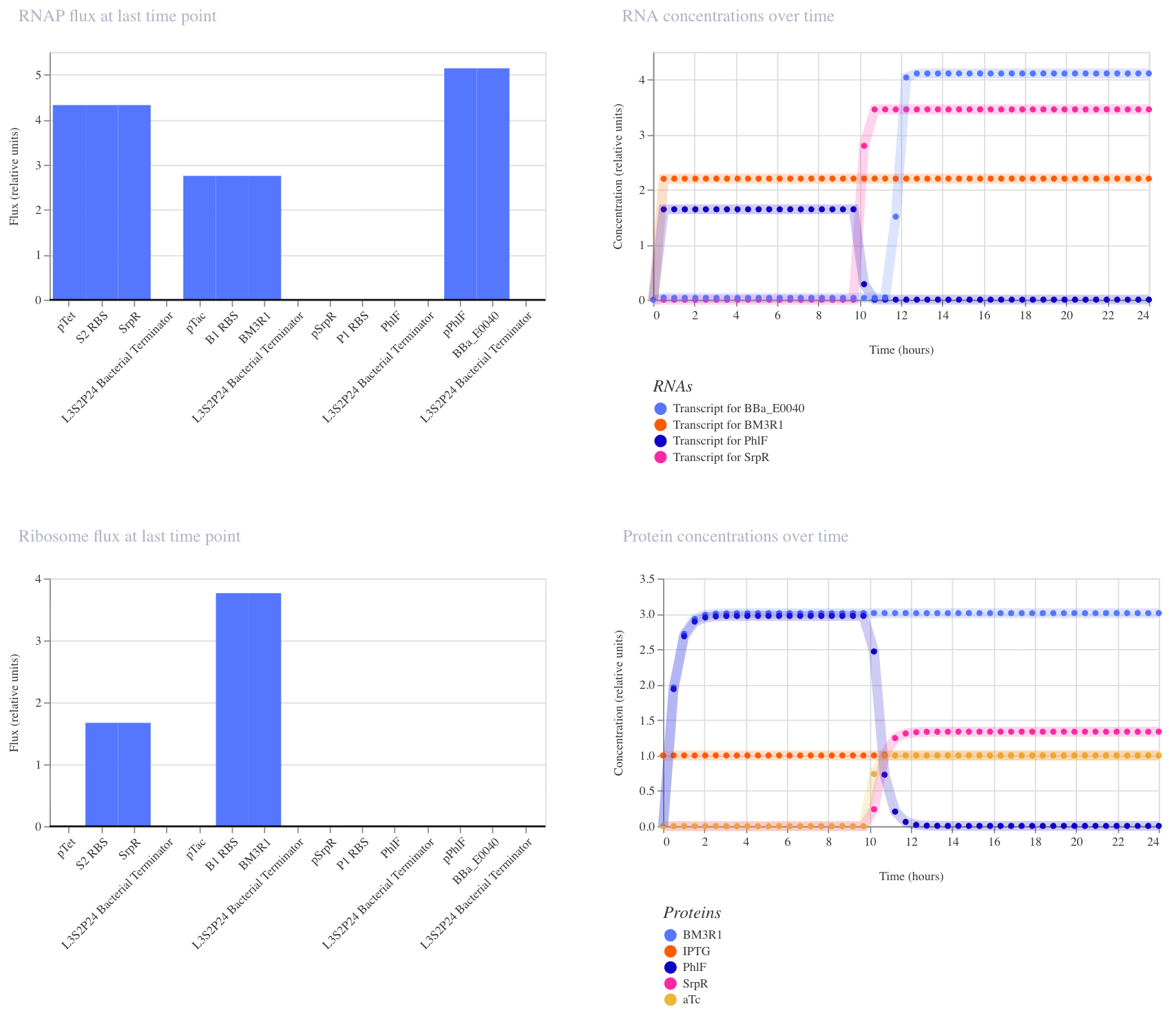
2. AND Gate

This construct implements two-input logic: GFP (BBa_E0040) is only produced when both aTc AND IPTG are present. The logic works through a double repression cascade: aTc induces SrpR and IPTG induces BM3R1, and both repressors are needed together to sufficiently suppress PhIF. Only when PhIF is low enough does pPhIF turn on and drive GFP expression. I expected GFP to remain off when only one input is present, and to switch on only when both inputs are active simultaneously.

I ran two simulations (E. coli, 24 hours, 30-minute timestep, transient transfection).

In the first run (aTc at hour 0, IPTG at hour 10), the results didn’t fully match expectations: GFP appeared elevated before both inputs were present, suggesting leakiness where one repressor alone was partially sufficient to suppress PhIF. This likely reflects imperfect repression strength in the cascade, which is a known limitation of cascaded repressor designs.

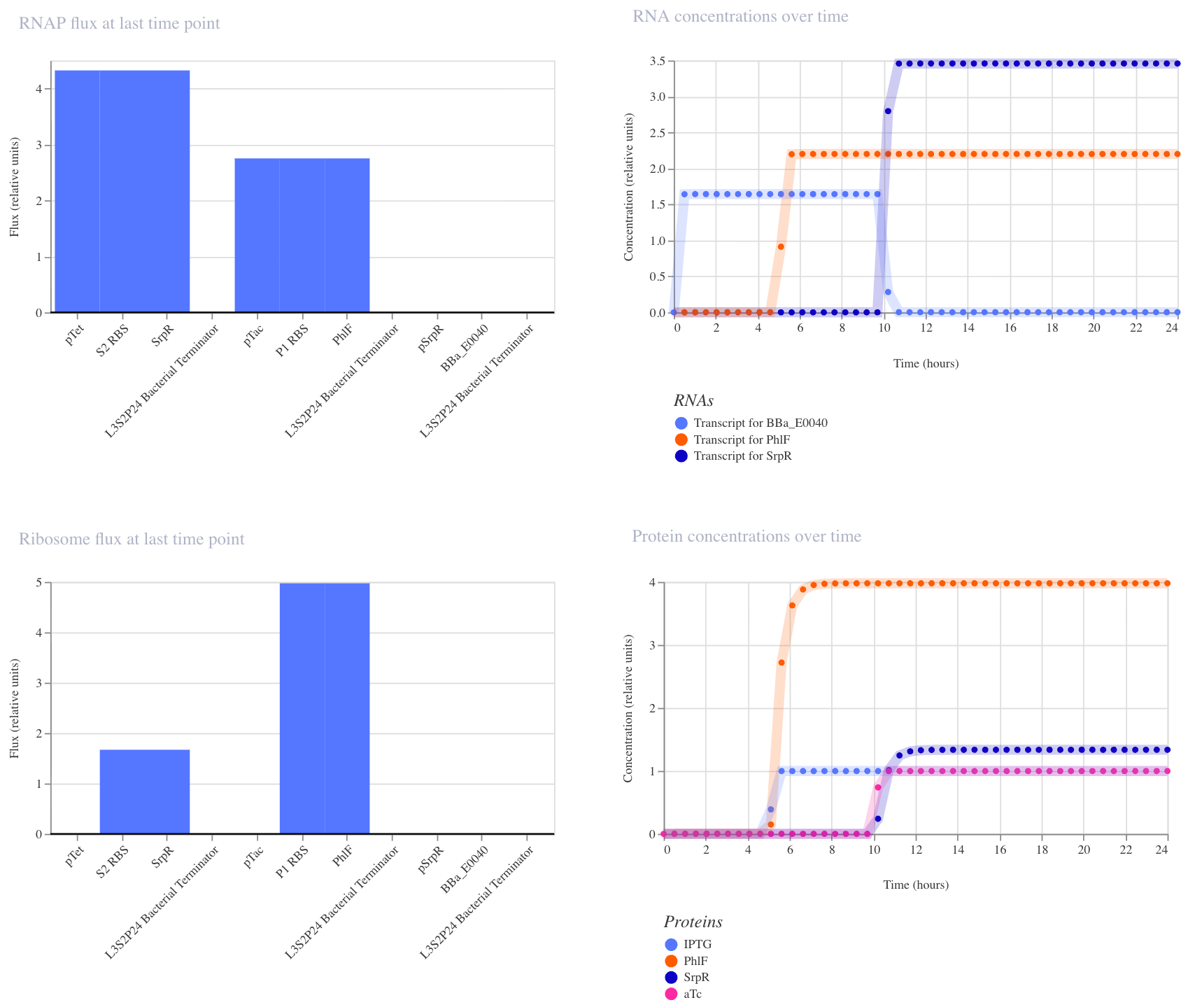
In the second run (IPTG at hour 0, aTc at hour 10), the expected AND gate behavior was clearly visible: GFP remained off until aTc arrived at hour 10, then switched on sharply. This confirms that both inputs are required for full GFP activation, and that the order of input delivery affects how cleanly the logic is observed.

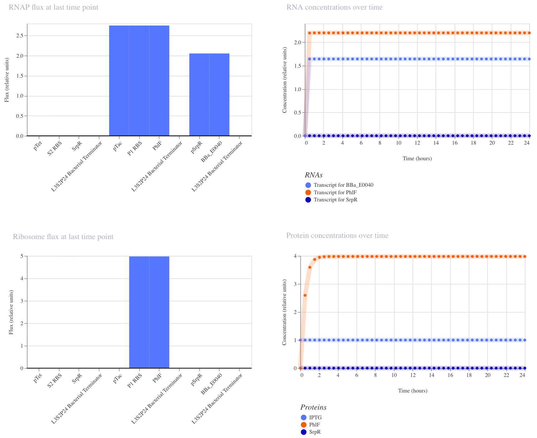
3. NAND Gate

This construct implements NAND logic: GFP (BBa_E0040) is ON by default and only turns off when both aTc AND IPTG are present. aTc induces SrpR via pTet, and IPTG induces PhIF via pTac. Only when both repressors are active simultaneously is pSrpR sufficiently repressed to turn off GFP. I expected GFP to be on in all conditions except when both inputs are present together.

I ran three simulations to test this (E. coli, 24 hours, 30-minute timestep, transient transfection).

With no inputs, GFP RNA was high (~1.7), confirming it is on by default.

With IPTG alone, GFP RNA remained high, confirming that a single input is insufficient to turn it off.

In the third run (IPTG at hour 5, aTc at hour 10), GFP RNA stayed high until aTc arrived at hour 10, at which point it dropped to near zero, confirming that both inputs together are required to turn GFP off. This matches the expected NAND behavior.

Week 7: Genetic Circuits Part II

Part 1: Intracellular Artificial Neural Networks

Q1. What advantages do IANNs have over traditional genetic circuits, whose input/output behaviors are Boolean functions?

Traditional genetic circuits are limited to discrete on/off outputs — a gene is either expressed or it isn’t. IANNs can compute analog, weighted combinations of inputs, which means the output can vary continuously depending on the relative strength of multiple signals. This allows a single cell to integrate many inputs simultaneously and produce graded responses, rather than being locked into binary logic. It also means that the same circuit architecture can be tuned to respond to different input combinations just by changing the weights, without redesigning the circuit from scratch.

Q2. Describe a useful application for an IANN; include a detailed description of input/output behavior, as well as any limitations an IANN might face to achieve your goal.

An IANN could be used for early cancer detection inside a cell — taking in multiple biomarker inputs (like elevated levels of specific transcription factors or oncoproteins) and only triggering a reporter output when the weighted combination exceeds a threshold. The input would be endogenous molecular concentrations, and the output would be something like a fluorescent signal or apoptosis trigger. The limitation is that biological noise inside a cell is high, so the weights are hard to set precisely, and the system might fire incorrectly if any one input fluctuates. Translating a trained weight matrix into actual RNA/protein concentrations is also not straightforward.

Q3. Multilayer perceptron diagram

The diagram shows an intracellular two-layer perceptron. In this circuit:

• X1 = DNA encoding Csy4 (endoribonuclease, Layer 1 inhibitor)
• X2 = DNA encoding Csy4_rec_CasE (CasE mRNA with Csy4 recognition hairpins, Layer 1 output)
• B1 = DNA encoding CasE_rec_mNeonGreen (mNeonGreen mRNA with CasE recognition hairpins, Layer 2 output)
• Blue circle = mNeonGreen fluorescent protein (final output)

When X1 is active, Csy4 cleaves the Csy4_rec_CasE mRNA so no CasE is produced, leaving the CasE_rec_mNeonGreen mRNA intact in Layer 2 and allowing mNeonGreen to be translated — the cell glows only when X1 suppresses the intermediate layer.

Part 2: Fungal Materials

Q1. What are some examples of existing fungal materials and what are they used for? What are their advantages and disadvantages over traditional counterparts?

Mycelium-based composites are probably the most well-known example — companies like Ecovative grow fungal networks on agricultural waste to make packaging foam and leather alternatives like Bolt Threads’ Mylo. They’re biodegradable and low carbon footprint compared to plastic foam or animal leather, but mechanical consistency is hard to control at scale and they’re still slower to produce than conventional manufacturing.

Chitosan, most commonly extracted from crustacean shells, can also be derived from fungal cell walls — and the fungal version is gaining interest as a vegan, seafood-free alternative for biodegradable films, wound dressings, and antimicrobial textile coatings. It’s biocompatible and compostable compared to synthetic polymer coatings, but fungal extraction yields are currently much lower than crustacean sources, and the material can be brittle without plasticizers.

Fungal pigments are a lesser-known but really interesting case — species like Monascus produce deep reds and Isaria produces yellows that are being explored as natural textile dyes. Compared to synthetic dyes, they’re biodegradable and less toxic, but yield is low, color consistency batch-to-batch is tricky, and lightfastness is generally worse than synthetic alternatives.

Q2. What might you want to genetically engineer fungi to do and why? What are the advantages of doing synthetic biology in fungi as opposed to bacteria?

I’d want to engineer fungi to secrete specific structural proteins — like silk or reflectin-like proteins — directly into the mycelium matrix as it grows, so the material self-assembles with tunable optical or mechanical properties built in. This is interesting for wearables because you could grow a material that is already functionalized rather than coating it afterward. The reason to use fungi over bacteria here is that fungi are eukaryotes, so they can handle larger, more complex proteins with proper folding and post-translational modifications that bacteria often struggle with. They also naturally grow into 3D fibrous networks, which means you get macroscale structure for free — bacteria just make a liquid culture you then have to process separately.

Week 9: Cell-Free Protein Expression

Part A: General Questions

Q1. Explain the main advantages of cell-free protein synthesis over traditional in vivo methods, specifically in terms of flexibility and control over experimental variables. Name at least two cases where cell-free expression is more beneficial than cell production.

Cell-free systems can be freeze-dried and reactivated through hydration, making them deployable outside of a wet lab without refrigeration or live cell maintenance or biosafety issues. This opens up applications that in vivo systems simply can’t reach: (1) toxic proteins that would kill a living host can be expressed safely; (2) materials embedded with biological sensing or production capacity like textiles or wound dressings where living cells are not practical.

Q2. Describe the main components of a cell-free expression and role of each component.

Cell lysate provides the ribosomes, translation factors, RNA polymerase, and other endogenous machinery needed for transcription and translation. DNA template is the gene of interest to be expressed. An energy regeneration system (like phosphocreatine + creatine kinase) continuously regenerates ATP to power the reaction. Amino acids are the building blocks for the protein. Salts and buffers maintain optimal pH and ionic conditions to keep conditions stable for expression.

Q3. Why is energy provision regeneration critical in cell-free systems? Describe a method you could use to ensure continuous ATP supply in your cell-free experiment.

Cell-free reactions consume ATP rapidly and have no metabolism to regenerate it, so the reaction stalls quickly without a continuous supply. A common method is the phosphocreatine/creatine kinase system: creatine kinase transfers a phosphate group from phosphocreatine to ADP, regenerating ATP. An alternative is the maltose/maltose binding protein system which uses sugar metabolism to drive ATP regeneration over longer timescales.

Q4. Compare prokaryotic versus eukaryotic cell-free expression systems. Choose a protein to produce in each system and explain why.

Prokaryotic systems (like E. coli lysate) are cheaper, faster to prepare, and have higher yields which means they are good for simple soluble proteins. Eukaryotic systems (like wheat germ or HeLa cell lysate) support post-translational modifications like glycosylation and disulfide bond formation. A bacterial enzyme like Cas9 can be produced in a prokaryotic system since it doesn’t require post-translational modifications and benefits from high yield. Human antibodies can be produced in a eukaryotic system since proper glycosylation is critical for its function and stability.

Q5. How would you design a cell-free experiment to optimize the expression of a membrane protein? Discuss the challenges and how you would address them in your setup.

Membrane proteins are challenging because they are hydrophobic and aggregate easily without a lipid environment. I would supplement the cell-free reaction with nanodiscs or liposomes to provide a membrane-like environment for the protein to fold into as it’s being synthesized. Detergents can also be added at sub-CMC concentrations to stabilize the protein without denaturing it. Yield would be optimized by titrating Mg2+ and K+ concentrations, and the protein would be assessed by SDS-PAGE and a functional binding assay rather than just fluorescence, since aggregation can give a false positive for expression.

Q6. Imagine you observe a low yield of your target protein in a cell-free system. Describe three possible reasons for this and suggest a troubleshooting strategy for each.

First, the DNA template concentration may be too low or the template may be degraded which would need to run a gel to check template integrity and titrate DNA concentration across a range to find the optimum. Second, the Mg2+ concentration may be off (critical cofactor for ribosomes and polymerases) so I would run a Mg2+ optimization grid. Third, the protein may be expressed but insoluble and aggregating, I would run both soluble and total fractions on SDS-PAGE separately to check whether the protein is being made but crashing out, and if so, add chaperones or adjust the reaction temperature to slow translation and allow proper folding.

Week 10: Imaging and Measurement

Final Project

Aspects of measurement

My final project, “Visible Emotion,” is a cell-free cortisol biosensor that outputs a spatial fluorescence gradient on filter paper. A constitutive T7-LuxI sender produces AHL, which diffuses outward and activates a dual-color receiver array: mVenus (low threshold, yellow) and mScarlet3 (high threshold, red). In Aim 2, the constitutive sender is replaced by a cortisol-responsive circuit: sweat cortisol binds a DNA aptamer, releasing a trigger strand that activates a toehold switch driving LuxI, linking stress level to the color gradient.

1. Spatial fluorescence gradient: Fluorescence intensity of mVenus and mScarlet3 as a function of distance from the AHL source. I will image the substrate with a fluorescence microscope or gel documentation system using YFP and RFP filter sets, then extract radial fluorescence intensity profiles in ImageJ (plot intensity vs. distance to sender spot curve for each channel). This follows the same imaging approach as Basu et al. 2005 (Nature 434, 1130), adapted from living cells on agar to cell-free on paper.

2. AHL diffusion: The diffusion distance determines the spatial extent of the fluorescence gradient. How far detectable fluorescence extends from the sender over time. Time-lapse fluorescence imaging at 1-2 hour intervals over 6-12 hours, measuring the radius of mVenus signal (extends further, low threshold) vs. mScarlet3 signal (confined closer, high threshold) using ImageJ.

3. pLux dose-response curve: Fluorescence output vs. AHL concentration for each receiver construct in 96-well plate format. Serial dilutions of synthetic AHL with known concentration (0 to 10 uM) added to cell-free reactions, measured by plate reader (mVenus: Ex 515/Em 528 nm; mScarlet3: Ex 569/Em 593 nm). This establishes the transfer function to understand at what AHL concentration does each reporter turn on and confirms the two constructs have different activation thresholds and dynamic range.

4. Cortisol cascade activation: Whether cortisol triggers the full aptamer → toehold → LuxI → AHL → receiver cascade. Two-stage plate reader assay: incubate hydrocortisone at varying concentrations with aptamer-toehold-LuxI cell-free reaction, then transfer to a pLux-mVenus receiver reaction. Cortisol dose-dependent mVenus fluorescence confirms the cascade is functional.

5. Protein expression verification: Gel electrophoresis of cell-free reaction products to confirm bands at expected molecular weights compared to a ladder (LuxR ~29 kDa, mVenus ~27 kDa, mScarlet3 ~26 kDa, LuxI ~25 kDa). Fluorescent proteins can also be visualized directly on unstained gels under blue light excitation.

Technologies summary: fluorescence microscopy, ImageJ, fluorescence plate reader, gel electrophoresis, gel documentation system.

Waters Part I — Molecular Weight

1. What is the calculated molecular weight of eGFP?

Unmodified MW: ~28,006.60 Da. With GFP chromophore maturation: the chromophore forms by cyclization of Ser65-Tyr66-Gly67, which loses one water molecule (-18.015 Da) and undergoes oxidation (-2.016 Da), for a net change of -20.031 Da. Predicted MW with chromophore: ~27,986.57 Da.

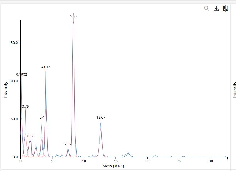
2. Calculate the molecular weight using the adjacent charge state approach.

I select from the intact LC-MS data:

• $\frac{m}{z_n}$ = 966.0390
• $\frac{m}{z_{n+1}}$ = 933.8391

Determine z for each adjacent pair of peaks (n, n+1):

$$z = \frac{\frac{m}{z_{n+1}}}{\frac{m}{z_n} - \frac{m}{z_{n+1}}}$$

$$z = \frac{933.8391}{966.0390 - 933.8391} = \frac{933.8391}{32.1999} = \textbf{29}$$

The peak at 966.0390 has charge state 29+ and the peak at 933.8391 has charge state 30+.

Calculate MW:

$$MW = z \times \frac{m}{z_n} - z \times 1.008$$

$$MW = 29 \times 966.0390 - 29 \times 1.008 = 28{,}015.13 - 29.23 = \textbf{27,985.9 Da}$$

Calculate the accuracy of the measurement:

$$Accuracy = \frac{|MW_{experiment} - MW_{theory}|}{MW_{theory}}$$

$$Accuracy = \frac{|27985.9 - 27986.6|}{27986.6} = \mathbf{4.29 \times 10^{-5}}$$

In ppm: $4.29 \times 10^{-5} \times 10^{6}$ = ~43 ppm.

3. Can you observe the charge state for the zoomed-in peak?

Yes, the charge state can be determined: 19+ charge state. This can be found by counting from the charge states already determined in Q2, and assigning each successive peak one fewer charge moving to the right, which places the peak at m/z ≈ 1474 at 19+. In the zoomed view, isotope peaks are partially visible but it’s difficult to count the number of peaks and the signal is somewhat noisy at this m/z spacing (1/19 = 0.053 m/z). The instrument’s 30,000 resolution is just sufficient to begin resolving isotope peaks at this charge state (required resolution: 1474/0.053 ≈ 27,800).

Waters Part II — Secondary/Tertiary Structure

1. Explain the difference between native and denatured protein conformations.

When a protein unfolds (denatures), its compact 3D structure opens up into an extended, disordered chain. For eGFP, this means the beta-barrel collapses, the chromophore environment is disrupted, and the protein loses its fluorescence.

In the mass spectrometer, this is detected through the charge state distribution.

• Native (folded): the protein is compact, so fewer surface-accessible sites are available for protonation. It picks up fewer charges per molecule, shifting the charge state envelope to higher m/z values (right side of spectrum). You see fewer, tighter peaks.
• Denatured (unfolded): the protein is extended, exposing more basic residues to protonation. This produces more charges per molecule, shifting the envelope to lower m/z values (left side of spectrum). You see more peaks spread across a broader range.

2. Can you discern the charge state of the peak at ~2800 m/z?

Looking at the zoomed view, the spacing between isotope peaks = $1/z$.

$$z = \frac{1}{2545.2222 - 2545.1304} = \frac{1}{0.0918} \approx \textbf{11}$$

Waters Part III — Peptide Mapping

1. How many Lysines (K) and Arginines (R) are in eGFP?

Lysine (K): 20 residues. Arginine (R): 6 residues. Total K + R: 26.

2. How many peptides will be generated from tryptic digestion?

Using the ExPASy PeptideMass tool (https://web.expasy.org/peptide_mass/) with the parameters in Figure 4: 19 peptides

3. How many chromatographic peaks in the eGFP peptide map (Figure 5a)?

Between 0.5 and 6 minutes with >10% relative abundance, approximately 22 peaks

Q4. Does the number of peaks match the predicted peptide count?

There are more peaks (22) than predicted peptides (19). Reasons: missed cleavages produce additional longer peptide species (the expected fragments and the uncut fragment as separate peaks), the chromophore modification creates a mass variant of the peptide containing residues 65-67, and trypsin autolysis fragments contribute additional peaks.

5. Identify the peptide at 2.78 minutes (Figure 5b).

The most abundant peak is at $\frac{m}{z}$ = 525.76712. Looking at the isotope peak spacing in the inset: 526.25918 − 525.76712 = 0.492, so charge $z = 1/0.492$ = 2+.

Calculate the singly charged mass $[M+H]^+$:

$$[M+H]^+ = \frac{m}{z} \times z - 1 \times 1.008$$

$$[M+H]^+ = 525.767 \times 2 - 1 \times 1.008 = 1051.534 - 1.008 = \mathbf{1050.526\ Da}$$

6. Identify the peptide and calculate mass accuracy.

Comparing 1050.526 Da to the predicted tryptic peptide list from the PeptideMass tool, this matches FEGDTLVNR (predicted $[M+H]^+$ = 1050.5214 Da).

$$PPM\ error = \frac{|1050.526 - 1050.521|}{1050.521} \times 10^{6} \approx \mathbf{4.6\ ppm}$$

7. What is the percentage of sequence confirmed by peptide mapping?

88% sequence confirmed by peptide mapping.

Waters Part IV — KLH Oligomers

Identify the oligomeric species on the CDMS spectrum.

Waters Part V — Did I Make GFP?