from opentrons import types
import string
metadata = {
'protocolName': '{ANNIE} - Opentrons Art - HTGAA',
'author': 'HTGAA',
'source': 'HTGAA 2026',
'apiLevel': '2.20'
}
Z_VALUE_AGAR = 2.0
POINT_SIZE = 0.75
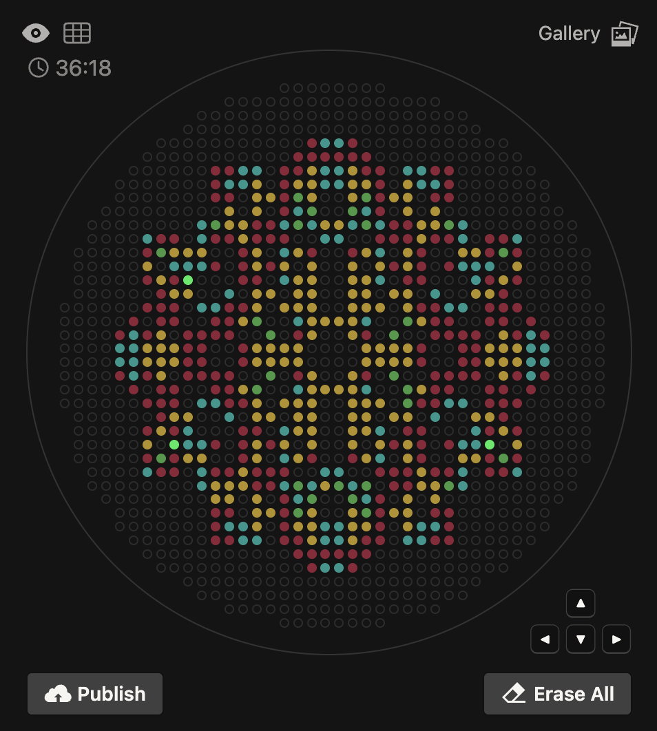
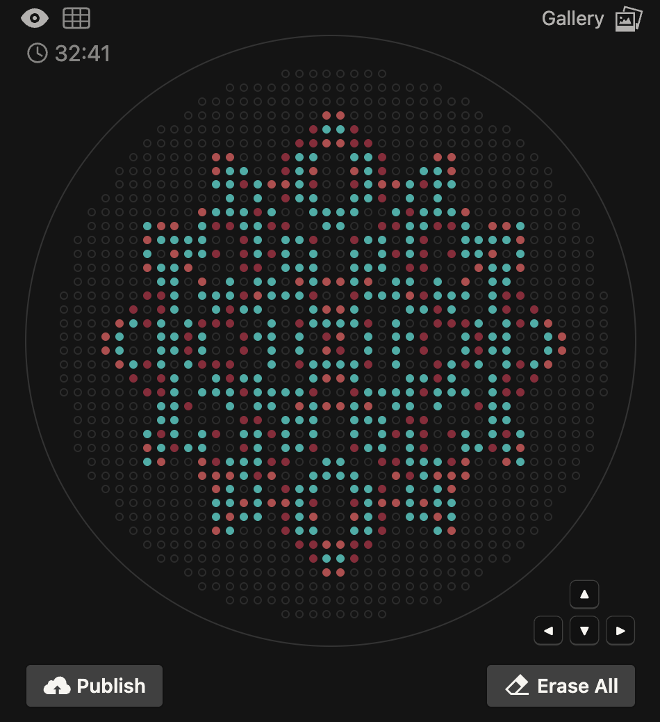
mjuniper_points = [(-1,31), (1,31), (-13,27), (-11,27), (-1,27), (1,27), (11,27), (13,27), (-15,25), (-13,25), (-1,25), (1,25), (13,25), (15,25), (-5,21), (5,21), (-19,19), (-7,19), (-3,19), (3,19), (7,19), (19,19), (-27,17), (-19,17), (-1,17), (1,17), (19,17), (27,17), (-7,15), (7,15), (-23,13), (-21,13), (-19,13), (19,13), (21,13), (23,13), (-7,11), (7,11), (21,11), (-15,9), (15,9), (-19,7), (-17,7), (17,7), (19,7), (-5,5), (5,5), (-29,3), (29,3), (-31,1), (-29,1), (29,1), (31,1), (-31,-1), (-29,-1), (29,-1), (31,-1), (-29,-3), (29,-3), (-5,-5), (5,-5), (-19,-7), (-17,-7), (17,-7), (19,-7), (-15,-9), (15,-9), (-21,-11), (-7,-11), (7,-11), (21,-11), (-21,-13), (-19,-13), (19,-13), (21,-13), (-7,-15), (7,-15), (-27,-17), (-19,-17), (-1,-17), (1,-17), (19,-17), (27,-17), (-19,-19), (-7,-19), (-3,-19), (3,-19), (19,-19), (-5,-21), (5,-21), (-15,-25), (-13,-25), (-1,-25), (1,-25), (13,-25), (15,-25), (-13,-27), (-11,-27), (-1,-27), (1,-27), (11,-27), (13,-27), (-1,-31), (1,-31)]
mko2_points = [(-3,27), (3,27), (-11,25), (-5,25), (-3,25), (3,25), (5,25), (11,25), (-11,23), (-9,23), (-3,23), (3,23), (9,23), (11,23), (-15,21), (-11,21), (11,21), (15,21), (-15,19), (-13,19), (-1,19), (1,19), (13,19), (15,19), (-13,17), (13,17), (-23,15), (-21,15), (-19,15), (-11,15), (-5,15), (5,15), (11,15), (19,15), (21,15), (-27,13), (-11,13), (-7,13), (-3,13), (3,13), (7,13), (11,13), (27,13), (-25,11), (-5,11), (-3,11), (3,11), (5,11), (25,11), (-23,9), (-21,9), (-11,9), (-9,9), (-5,9), (-3,9), (3,9), (5,9), (9,9), (11,9), (21,9), (23,9), (-11,7), (-7,7), (-5,7), (-3,7), (3,7), (5,7), (7,7), (11,7), (-13,5), (-3,5), (-1,5), (1,5), (3,5), (13,5), (-25,3), (-3,3), (3,3), (25,3), (-27,1), (-25,1), (-23,1), (-11,1), (-9,1), (-7,1), (-5,1), (5,1), (7,1), (9,1), (11,1), (23,1), (25,1), (27,1), (-27,-1), (-25,-1), (-23,-1), (-11,-1), (-9,-1), (-7,-1), (-5,-1), (5,-1), (7,-1), (9,-1), (11,-1), (23,-1), (25,-1), (27,-1), (-25,-3), (-3,-3), (3,-3), (25,-3), (-13,-5), (-3,-5), (-1,-5), (1,-5), (3,-5), (13,-5), (-11,-7), (-7,-7), (-5,-7), (-3,-7), (3,-7), (5,-7), (7,-7), (-23,-9), (-21,-9), (-11,-9), (-9,-9), (-5,-9), (-3,-9), (3,-9), (5,-9), (9,-9), (11,-9), (21,-9), (23,-9), (-25,-11), (-5,-11), (-3,-11), (3,-11), (5,-11), (25,-11), (-27,-13), (-11,-13), (-7,-13), (-3,-13), (3,-13), (7,-13), (11,-13), (27,-13), (-21,-15), (-19,-15), (-11,-15), (-5,-15), (5,-15), (11,-15), (19,-15), (21,-15), (-13,-17), (13,-17), (-17,-19), (-15,-19), (-13,-19), (-1,-19), (13,-19), (15,-19), (-17,-21), (-15,-21), (-11,-21), (11,-21), (15,-21), (-11,-23), (-9,-23), (-3,-23), (3,-23), (9,-23), (11,-23), (-11,-25), (-5,-25), (-3,-25), (3,-25), (5,-25), (11,-25), (-3,-27), (3,-27)]
mrfp1_points = [(-3,31), (3,31), (-5,29), (-3,29), (-1,29), (1,29), (3,29), (5,29), (-17,27), (-15,27), (-7,27), (-5,27), (5,27), (7,27), (15,27), (17,27), (-17,25), (-7,25), (7,25), (17,25), (-17,23), (-15,23), (-7,23), (7,23), (15,23), (17,23), (-7,21), (7,21), (-11,19), (-9,19), (9,19), (11,19), (-25,17), (-23,17), (-17,17), (-15,17), (-11,17), (-9,17), (-7,17), (7,17), (9,17), (11,17), (15,17), (17,17), (23,17), (25,17), (-27,15), (-13,15), (-3,15), (3,15), (13,15), (23,15), (27,15), (-17,13), (-13,13), (-9,13), (9,13), (13,13), (17,13), (-27,11), (-23,11), (-13,11), (-11,11), (11,11), (13,11), (23,11), (27,11), (-25,9), (25,9), (-27,7), (-25,7), (-23,7), (-15,7), (-13,7), (13,7), (15,7), (23,7), (25,7), (27,7), (-29,5), (-25,5), (-23,5), (-17,5), (-15,5), (15,5), (17,5), (23,5), (25,5), (29,5), (-31,3), (-27,3), (-21,3), (-19,3), (-17,3), (-15,3), (-5,3), (5,3), (15,3), (17,3), (19,3), (21,3), (27,3), (31,3), (-21,1), (-19,1), (-13,1), (13,1), (19,1), (21,1), (-21,-1), (-19,-1), (-13,-1), (13,-1), (19,-1), (21,-1), (-31,-3), (-27,-3), (-21,-3), (-19,-3), (-17,-3), (-15,-3), (-5,-3), (5,-3), (15,-3), (17,-3), (19,-3), (21,-3), (27,-3), (31,-3), (-29,-5), (-25,-5), (-23,-5), (-17,-5), (-15,-5), (15,-5), (17,-5), (23,-5), (25,-5), (29,-5), (-27,-7), (-25,-7), (-23,-7), (-15,-7), (-13,-7), (13,-7), (15,-7), (23,-7), (25,-7), (27,-7), (-25,-9), (25,-9), (-27,-11), (-23,-11), (-13,-11), (-11,-11), (11,-11), (13,-11), (23,-11), (27,-11), (-17,-13), (-13,-13), (-9,-13), (9,-13), (13,-13), (17,-13), (-27,-15), (-23,-15), (-13,-15), (-3,-15), (3,-15), (13,-15), (23,-15), (27,-15), (-25,-17), (-23,-17), (-17,-17), (-15,-17), (-11,-17), (-9,-17), (-7,-17), (7,-17), (9,-17), (11,-17), (15,-17), (17,-17), (23,-17), (25,-17), (-11,-19), (-9,-19), (9,-19), (11,-19), (-7,-21), (7,-21), (-17,-23), (-15,-23), (-7,-23), (7,-23), (15,-23), (17,-23), (-17,-25), (-7,-25), (7,-25), (17,-25), (-17,-27), (-15,-27), (-7,-27), (-5,-27), (5,-27), (7,-27), (15,-27), (17,-27), (-5,-29), (-3,-29), (-1,-29), (1,-29), (3,-29), (5,-29), (-3,-31), (3,-31)]
mclover3_points = [(-5,23), (5,23), (-3,21), (3,21), (-17,19), (-5,19), (5,19), (17,19), (-25,15), (25,15), (-11,5), (11,5), (-9,3), (9,3), (-9,-3), (9,-3), (-11,-5), (11,-5), (11,-7), (-25,-15), (25,-15), (-5,-19), (1,-19), (5,-19), (17,-19), (-3,-21), (3,-21), (-5,-23), (5,-23)]
sfgfp_points = [(-21,11), (-23,-13), (23,-13)]
point_name_pairing = [("mjuniper", mjuniper_points),("mko2", mko2_points),("mrfp1", mrfp1_points),("mclover3", mclover3_points),("sfgfp", sfgfp_points)]
TIP_RACK_DECK_SLOT = 9
COLORS_DECK_SLOT = 6
AGAR_DECK_SLOT = 5
PIPETTE_STARTING_TIP_WELL = 'A1'
well_colors = {
'A1': 'sfGFP', 'A2': 'mRFP1', 'A3': 'mKO2', 'A4': 'Venus',
'A5': 'mKate2_TF', 'A6': 'Azurite', 'A7': 'mCerulean3', 'A8': 'mClover3',
'A9': 'mJuniper', 'A10': 'mTurquoise2', 'A11': 'mBanana', 'A12': 'mPlum',
'B1': 'Electra2', 'B2': 'mWasabi', 'B3': 'mScarlet_I', 'B4': 'mPapaya',
'B5': 'eqFP578', 'B6': 'tdTomato', 'B7': 'DsRed', 'B8': 'mKate2',
'B9': 'EGFP', 'B10': 'mRuby2', 'B11': 'TagBFP', 'B12': 'mChartreuse_TF',
'C1': 'mLychee_TF', 'C2': 'mTagBFP2', 'C3': 'mEGFP', 'C4': 'mNeonGreen',
'C5': 'mAzamiGreen', 'C6': 'mWatermelon', 'C7': 'avGFP', 'C8': 'mCitrine',
'C9': 'mVenus', 'C10': 'mCherry', 'C11': 'mHoneydew', 'C12': 'TagRFP',
'D1': 'mTFP1', 'D2': 'Ultramarine', 'D3': 'ZsGreen1', 'D4': 'mMiCy',
'D5': 'mStayGold2', 'D6': 'PA_GFP'
}
volume_used = {
'mjuniper': 0, 'mko2': 0, 'mrfp1': 0, 'mclover3': 0, 'sfgfp': 0
}
def update_volume_remaining(current_color, quantity_to_aspirate):
rows = string.ascii_uppercase
for well, color in list(well_colors.items()):
if color == current_color:
if (volume_used[current_color] + quantity_to_aspirate) > 250:
row = well[0]
col = well[1:]
next_row = rows[rows.index(row) + 1]
next_well = f"{next_row}{col}"
del well_colors[well]
well_colors[next_well] = current_color
volume_used[current_color] = quantity_to_aspirate
else:
volume_used[current_color] += quantity_to_aspirate
break
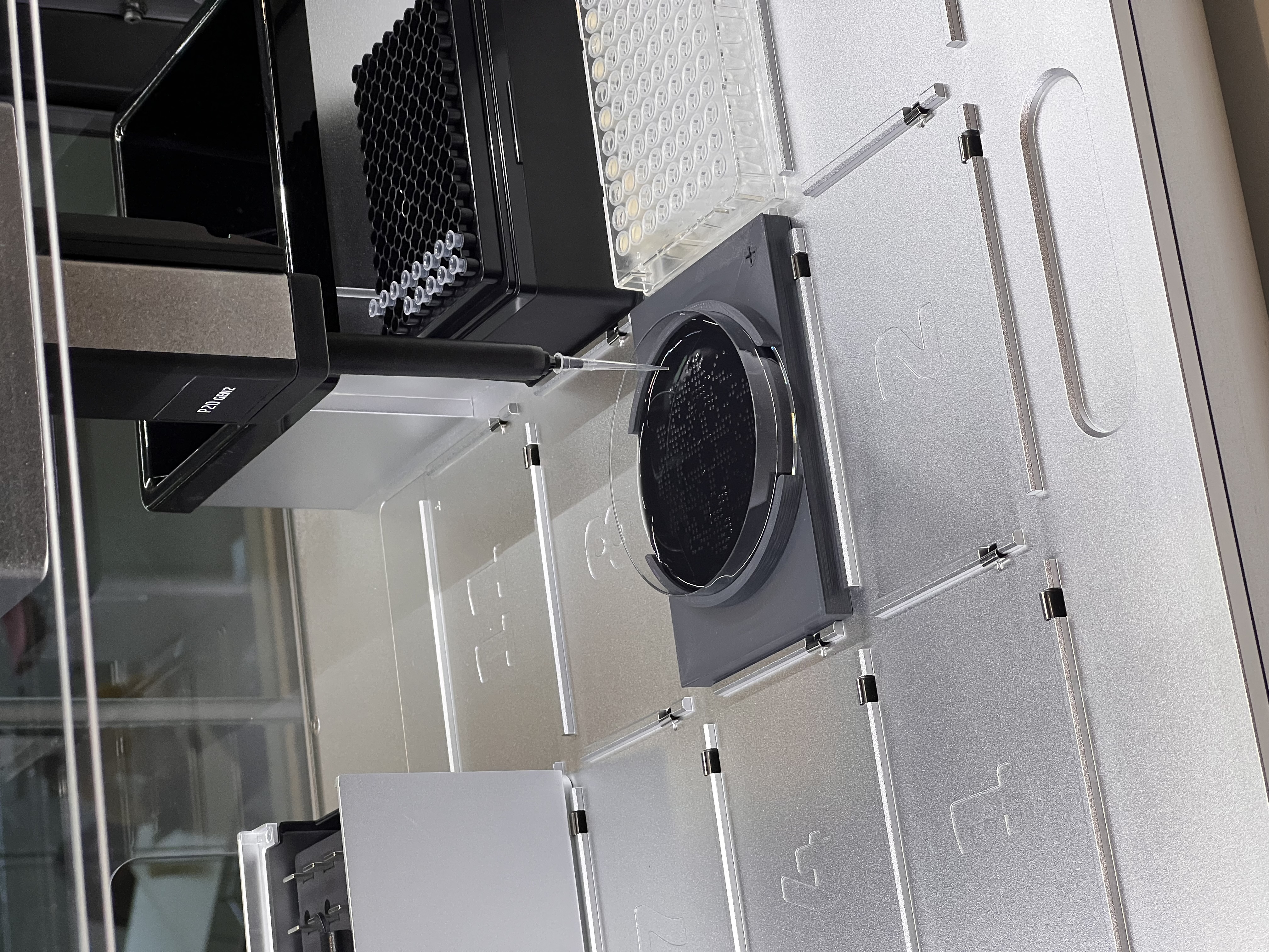
def run(protocol):
protocol.home()
tips_20ul = protocol.load_labware('opentrons_96_tiprack_20ul', TIP_RACK_DECK_SLOT, 'Opentrons 20uL Tips')
pipette_20ul = protocol.load_instrument("p20_single_gen2", "right", [tips_20ul])
temperature_plate = protocol.load_labware('opentrons_96_aluminumblock_generic_pcr_strip_200ul', 6)
agar_plate = protocol.load_labware('htgaa_agar_plate', AGAR_DECK_SLOT, 'Agar Plate')
agar_plate.set_offset(x=0.00, y=0.00, z=Z_VALUE_AGAR)
center_location = agar_plate['A1'].top()
pipette_20ul.starting_tip = tips_20ul.well(PIPETTE_STARTING_TIP_WELL)
def dispense_and_jog(pipette, volume, location):
assert(isinstance(volume, (int, float)))
above_location = location.move(types.Point(z=location.point.z + 2))
pipette.move_to(above_location)
pipette.dispense(volume, location)
pipette.move_to(above_location)
def location_of_color(color_string):
for well, color in well_colors.items():
if color.lower() == color_string.lower():
return temperature_plate[well]
raise ValueError(f"No well found with color {color_string}")
for i, (current_color, point_list) in enumerate(point_name_pairing):
if not point_list:
continue
pipette_20ul.pick_up_tip()
max_aspirate = int(18 // POINT_SIZE) * POINT_SIZE
quantity_to_aspirate = min(len(point_list)*POINT_SIZE, max_aspirate)
update_volume_remaining(current_color, quantity_to_aspirate)
pipette_20ul.aspirate(quantity_to_aspirate, location_of_color(current_color))
for i in range(len(point_list)):
x, y = point_list[i]
adjusted_location = center_location.move(types.Point(x, y))
dispense_and_jog(pipette_20ul, POINT_SIZE, adjusted_location)
if pipette_20ul.current_volume == 0 and len(point_list[i+1:]) > 0:
quantity_to_aspirate = min(len(point_list[i:])*POINT_SIZE, max_aspirate)
update_volume_remaining(current_color, quantity_to_aspirate)
pipette_20ul.aspirate(quantity_to_aspirate, location_of_color(current_color))
pipette_20ul.drop_tip()
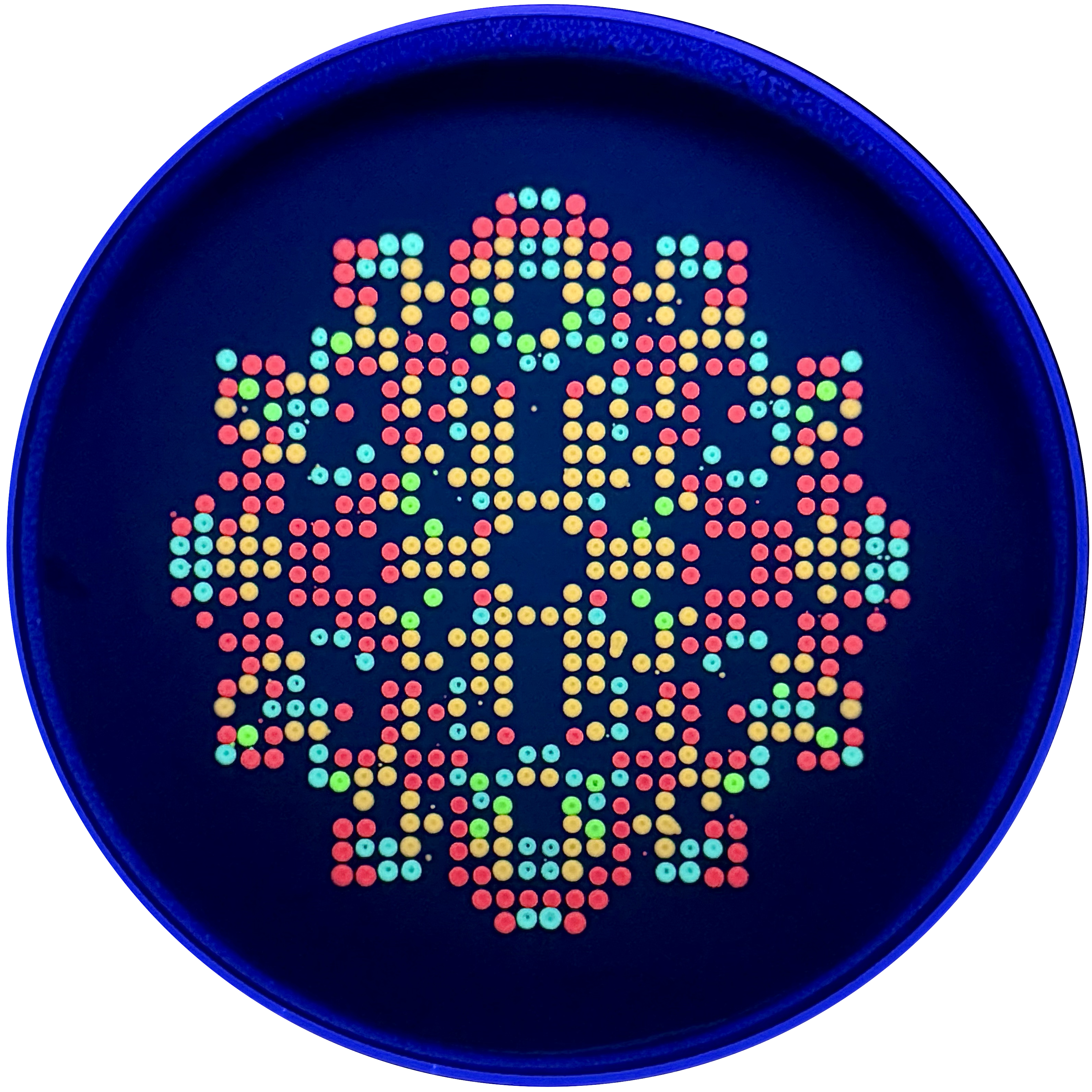
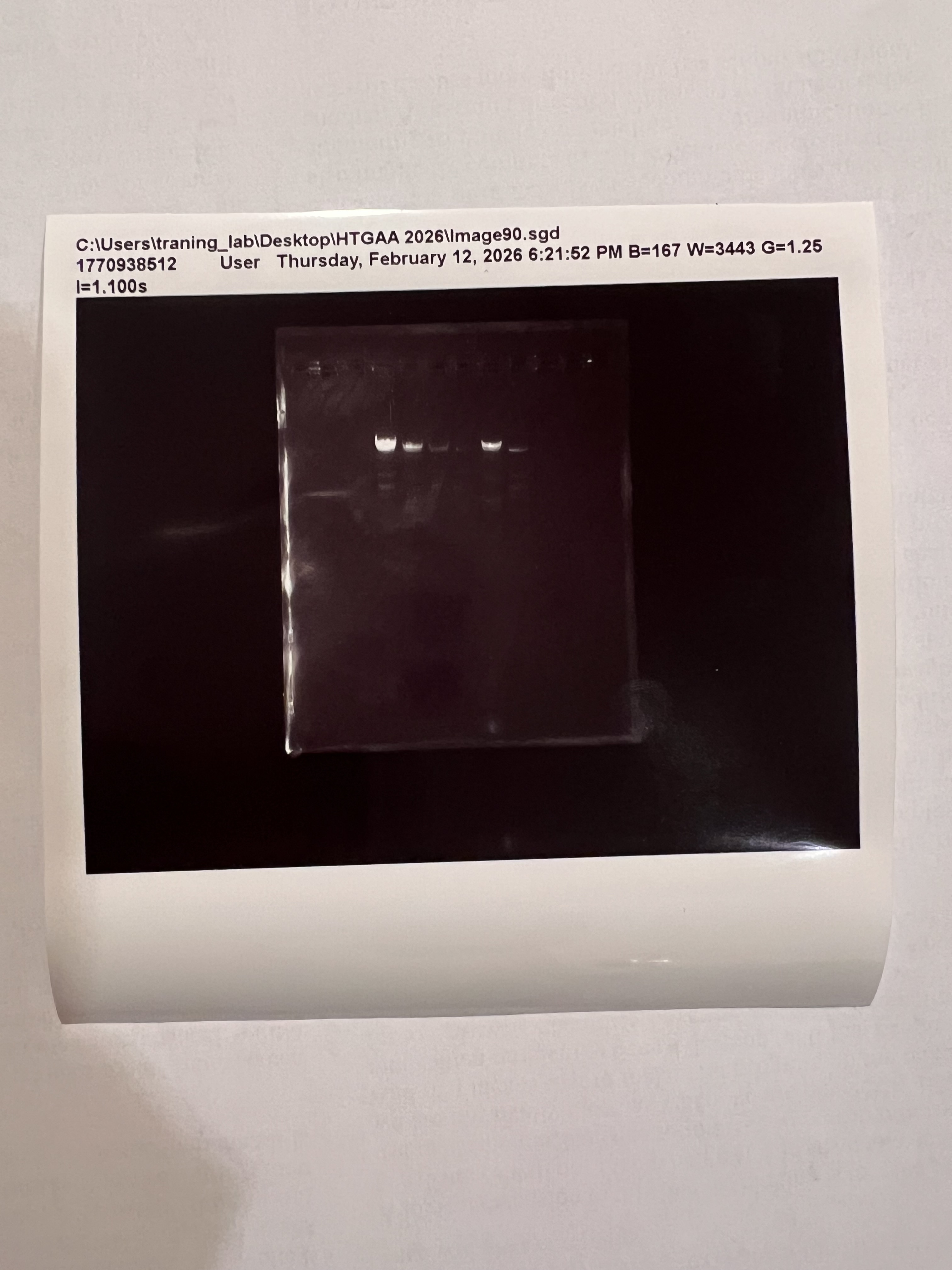
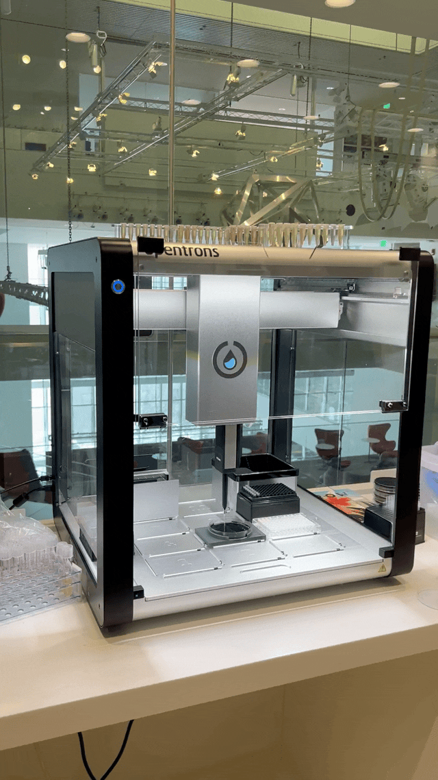
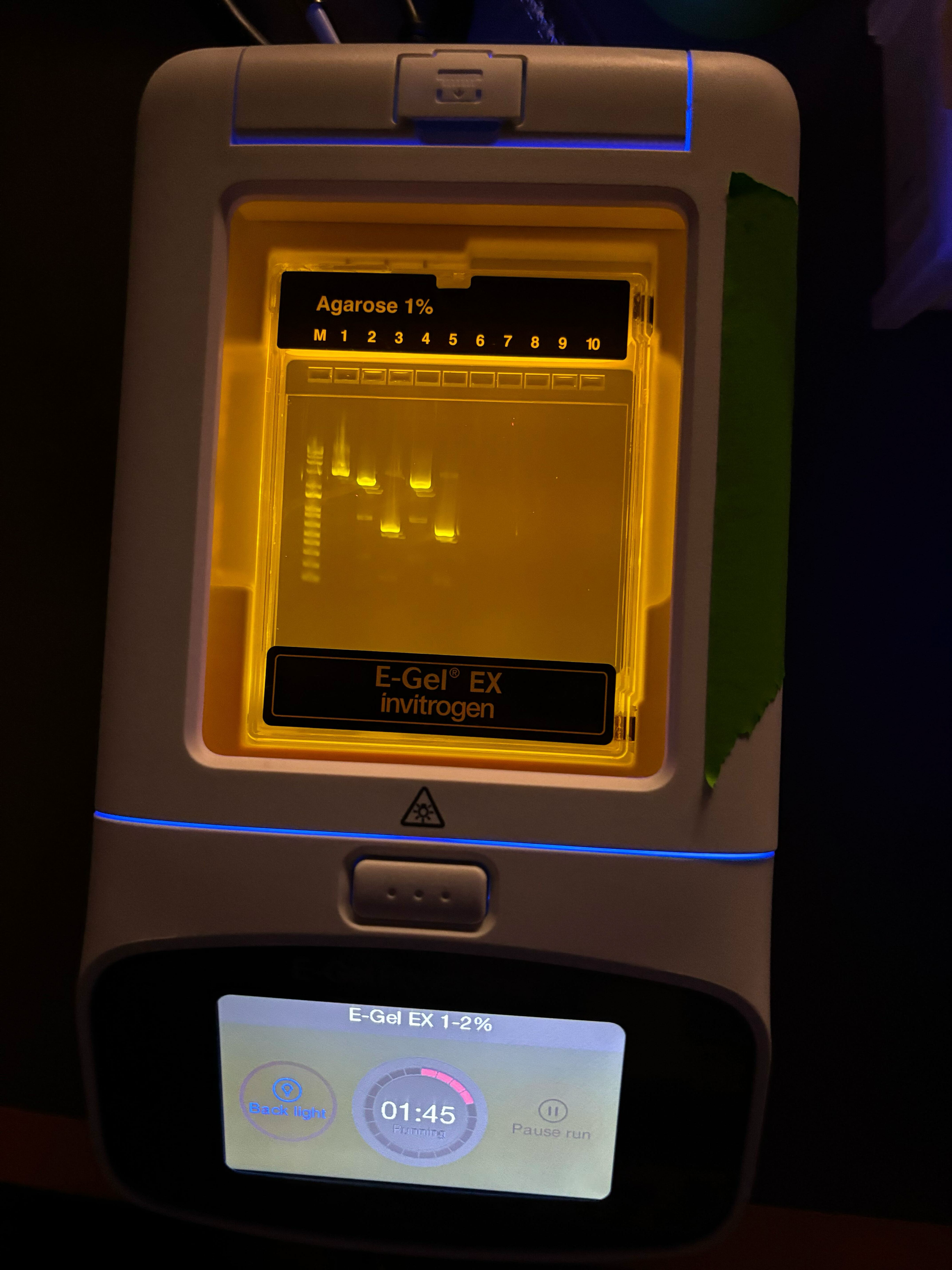
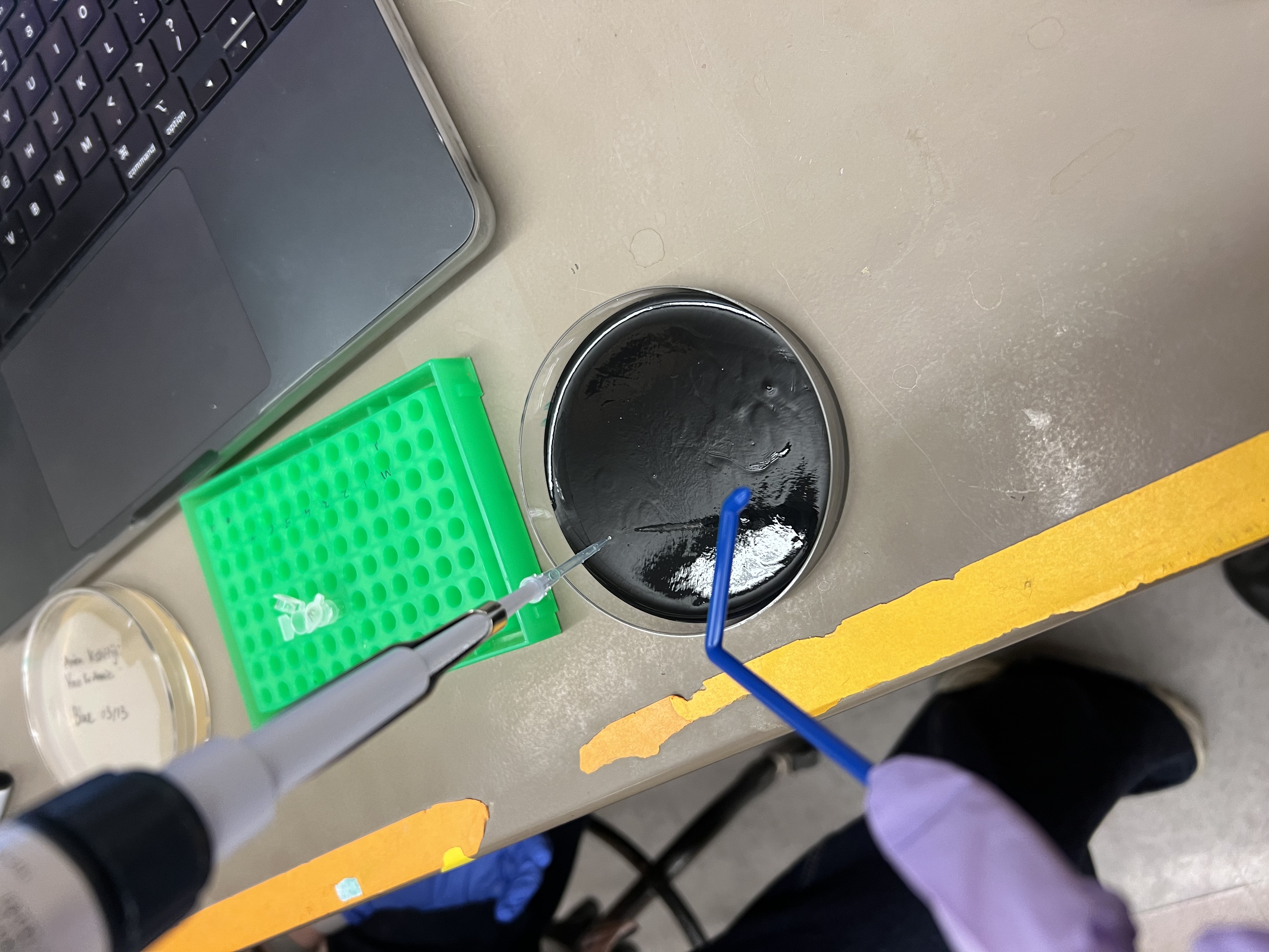
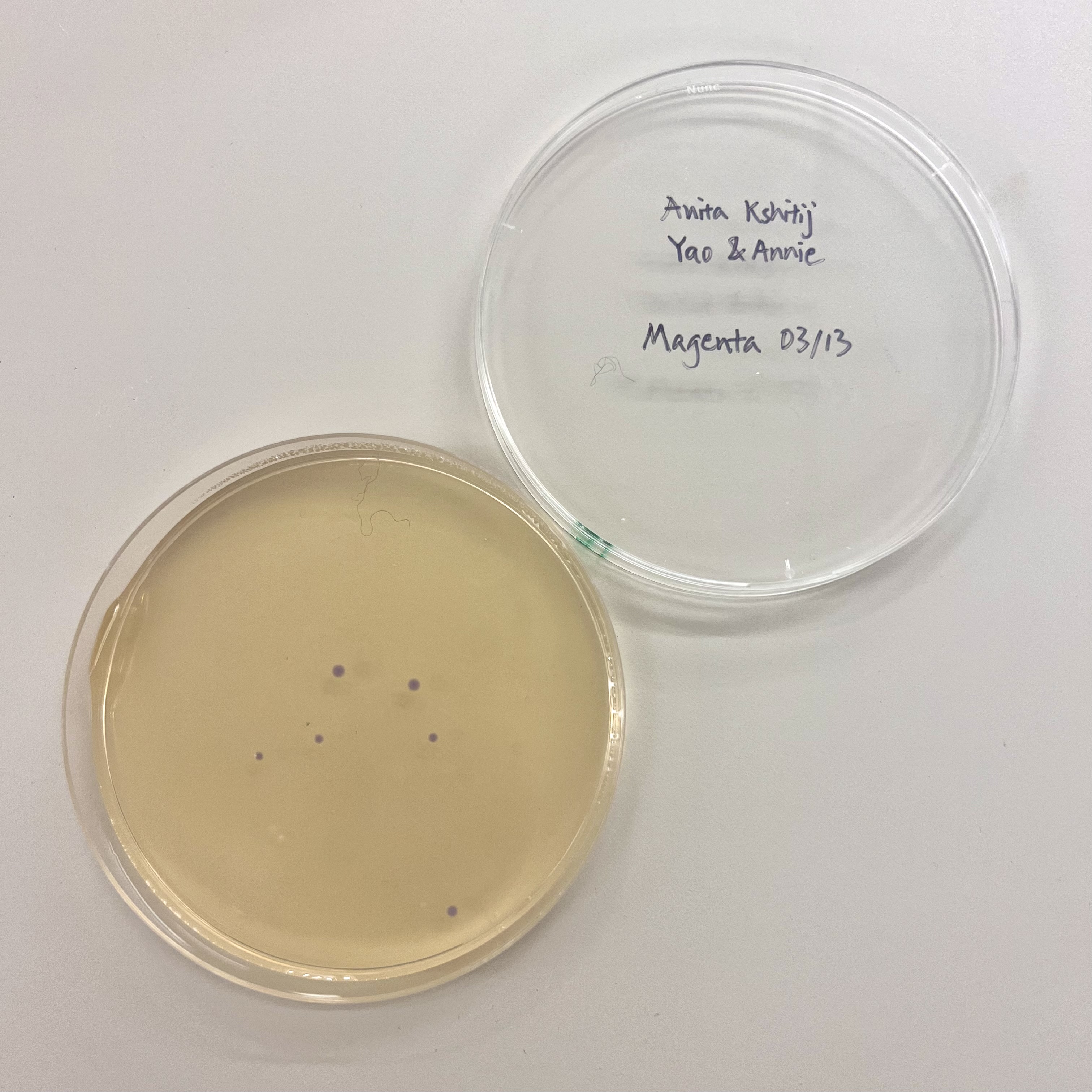
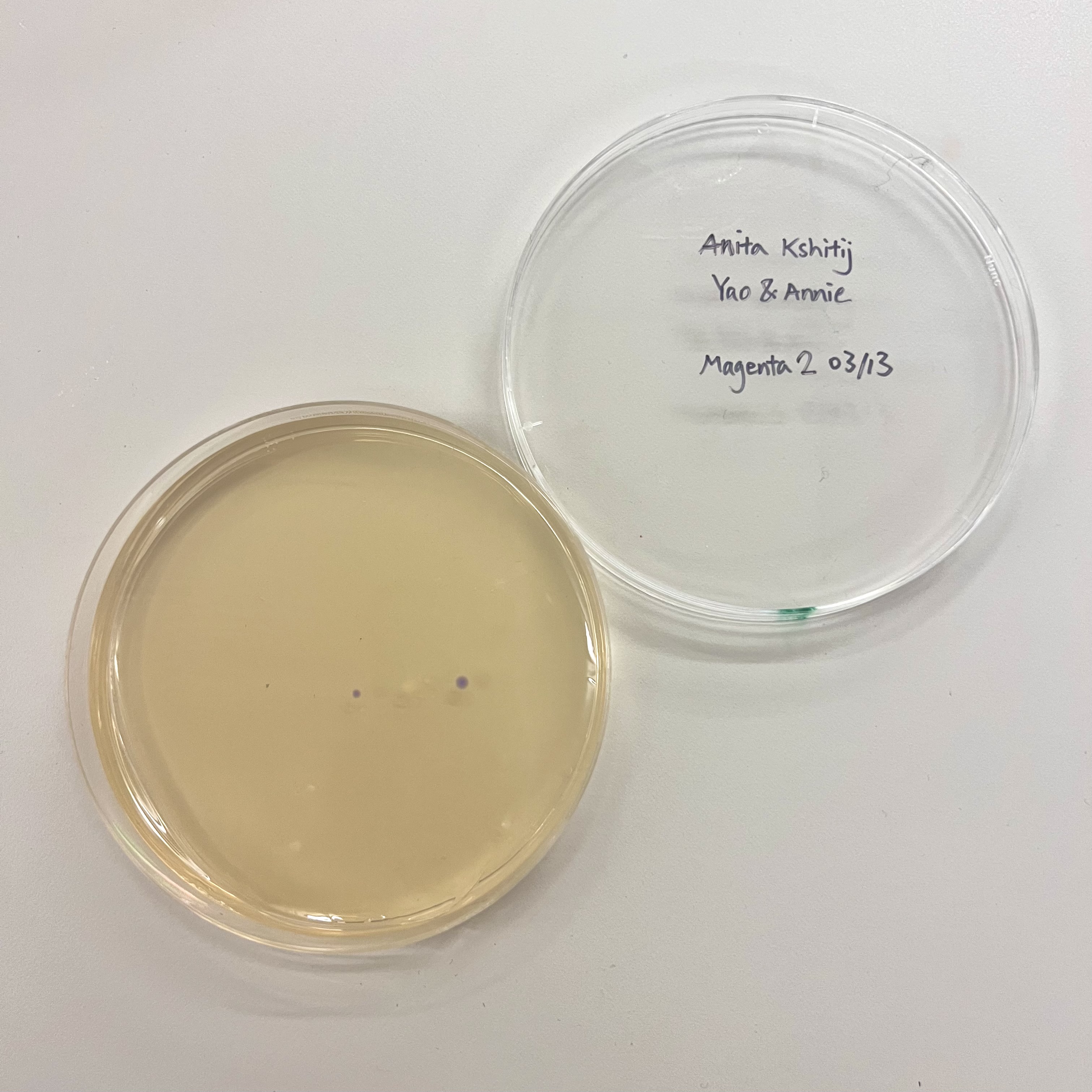
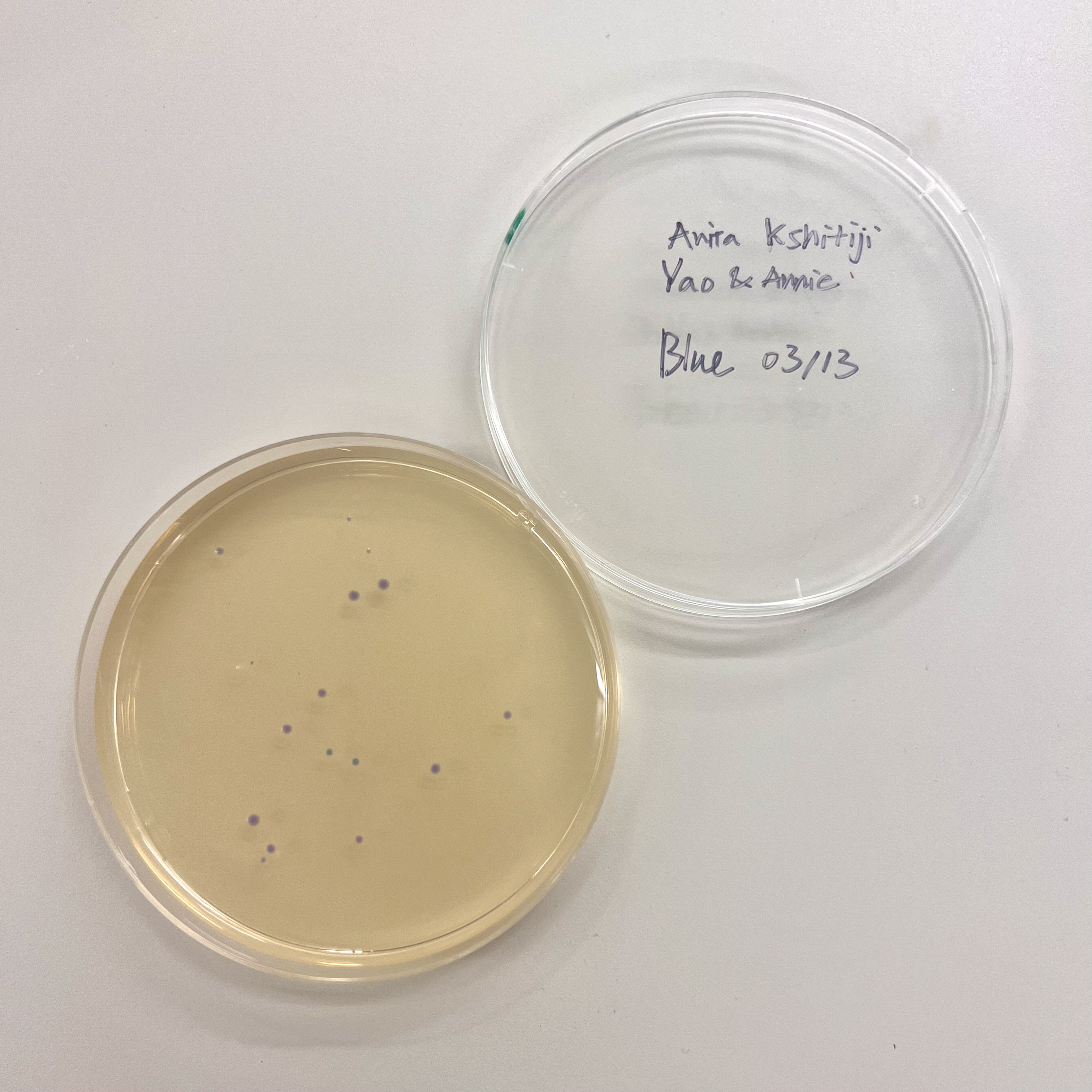
The OT-2 dispensed 0.75 µL drops of each fluorescent strain onto the charcoal agar plate.
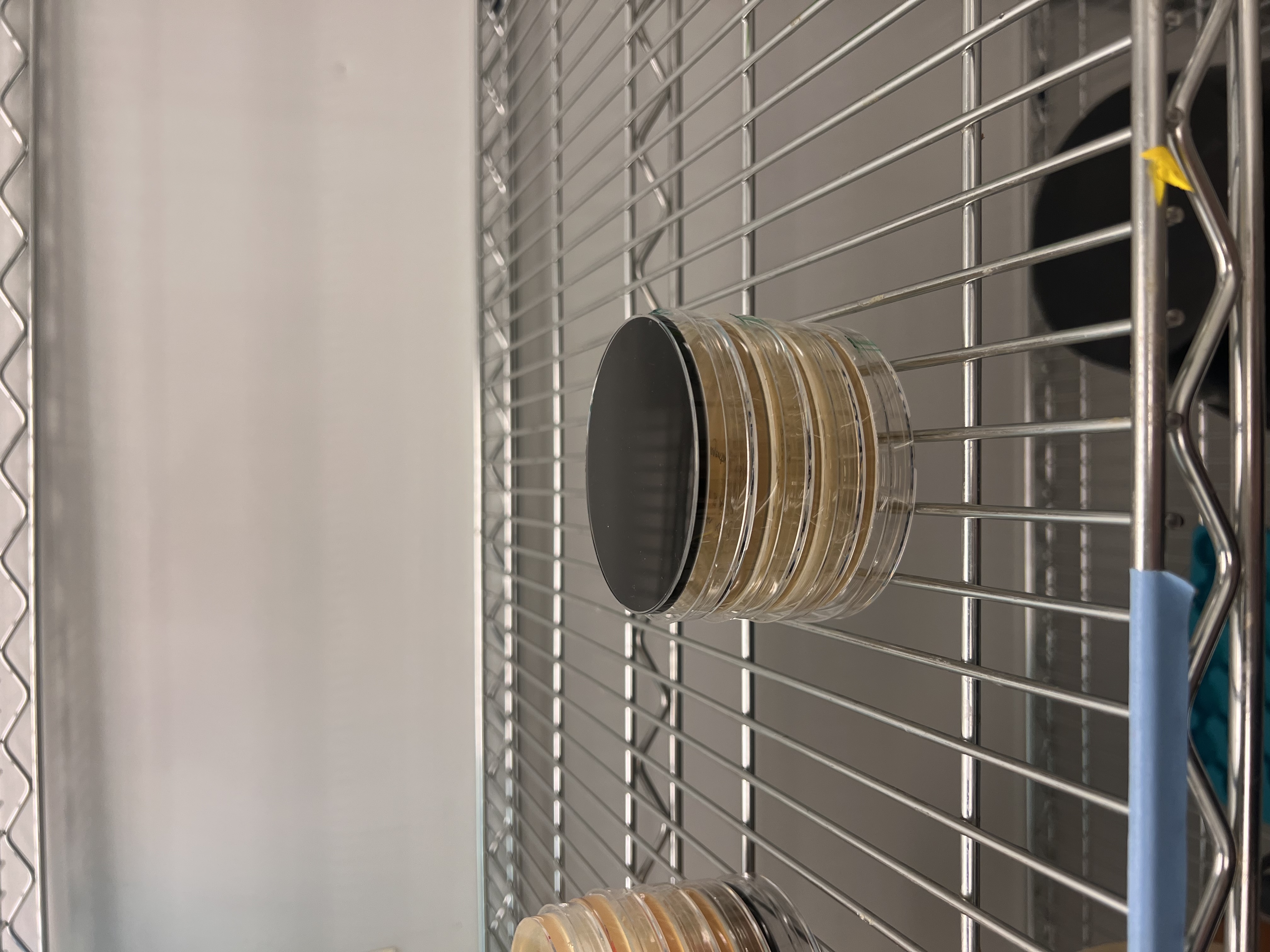
After overnight incubation, the plate was imaged under UV light.