Week 1 HW: Final Project Ideas

HTBAA Homework #1: Automated Biomanufacturing as a Discovery Engine for Biosensors

Course: How to Biomanufacture (Almost) Anything 2026 Assignment: Homework #1 — Biomanufacturing Proposal Due: Tuesday, September 22

1. What I Want to Biomanufacture, and Why

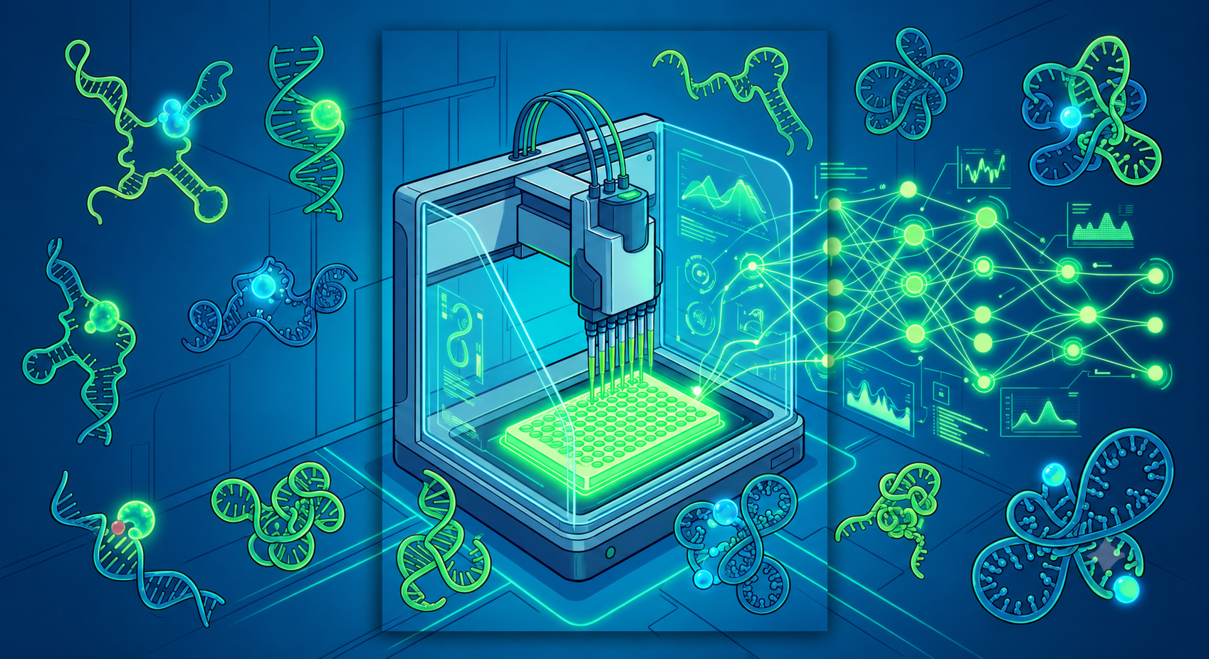
Most biosensor development treats “biomanufacturing” as the last step of the pipeline: once a laboratory has identified a promising aptamer or engineered protein switch, that molecule is scaled up and produced. My proposal inverts that relationship. I want to biomanufacture the biosensors themselves, but as the output of a closed, automated discovery loop in which biomanufacturing infrastructure is also the instrument that generates the data used to train and continually fine-tune the computational model that designs the sensors. In other words, the “product” is twofold: (i) a validated family of nucleic-acid (aptamer) and protein-based biosensors for a target class of analytes, and (ii) a progressively improving, experimentally grounded design model — a lab-in-the-loop system — that gets better at proposing new sensors with each iteration.

Motivation. Biosensor discovery today is bottlenecked by two disconnected worlds. On one side, structure- and sequence-based generative and predictive models (e.g., protein-language models, RNA structure predictors) can propose enormous numbers of candidate binders quickly and cheaply. On the other side, our ability to know whether a candidate actually binds a target analyte, with what affinity and specificity, still depends on comparatively slow, manual, low-throughput wet-lab assays (SELEX rounds, ELISA-type binding assays, biolayer interferometry). Asin-Garcia et al. (2025) argue that biomanufacturing more broadly is limited less by a lack of biological ideas than by a lack of research infrastructure that can consolidate automation, data, and expertise into reproducible pipelines. I want to apply that same infrastructural logic to biosensor discovery specifically: rather than manually deciding which experiment to run next, an automated pipeline should decide which data is missing, generate a protocol to acquire it, execute that protocol in an automated or cloud laboratory, and feed the result back into the model. This is directly motivated by, and would make direct use of, the specific case of trRosettaRNA2 (Wang, Peng and Yang, 2026), an RNA structure-prediction network that I examined as a template chassis for this idea (described in Section 2).

Who this is for. The intended beneficiaries are twofold: (a) practising biosensor developers (academic labs, diagnostics companies) who need custom aptamer/protein sensors for a novel analyte and currently must run SELEX or directed-evolution campaigns nearly from scratch each time; and (b) downstream users of the sensors — for instance, environmental monitoring programmes needing rapid, low-cost detection of an emerging contaminant class (e.g., per- and polyfluoroalkyl substances, PFAS) or public-health programmes needing point-of-care diagnostics for a metabolite panel. I think this is interesting/important because it reframes automated biomanufacturing not simply as a scale-up tool, but as a data-generation instrument for machine learning — the same conceptual shift that high-throughput “biofoundry” thinking has brought to strain engineering (Petzold and Mukhopadhyay, 2025) should be brought to affinity-reagent discovery, where public training data (e.g., existing aptamer/SELEX databases, RNA structure databases) is sparse relative to the size of chemical and sequence space that needs to be searched.

2. What Living System Would I Use?

I propose a cell-free transcription–translation (TX-TL) system, most likely derived from Escherichia coli lysate, as the primary chassis, complemented by an in vitro transcription system for RNA aptamer candidates. I choose a cell-free chassis over a whole living cell for three reasons, drawing on Karim and Jewett’s (2021) review of cell-free biomanufacturing: cell-free systems (i) have shorter development times because there is no strain-construction or transformation step between designing a sequence and testing it, (ii) tolerate reaction conditions and candidate molecules (including some that might be toxic or growth-inhibiting to a living cell) that would otherwise compromise cell viability, and (iii) their open reaction environment makes it straightforward to add an analyte directly to the reaction and read out a biosensor’s response in the same well, which is exactly what a screening-and-training loop requires.

High-level system description.

• Inputs: a linear DNA template (or plasmid) encoding a candidate aptamer or protein-based biosensor construct fused to a reporter (e.g., a fluorescent or luminescent output, or a riboswitch-controlled reporter gene for RNA aptamers); crude E. coli lysate containing the transcription/translation machinery; an energy/amino-acid/NTP master mix; and a dilution series of the target analyte (or a decoy panel of non-target molecules, to screen for specificity).
• Biological process: the cell-free extract transcribes and translates (or, for RNA aptamers, only transcribes) the candidate sequence. If the candidate is a functional biosensor, analyte binding alters folding or allosteric behaviour in a way that is coupled to the reporter signal (e.g., a fluorogenic aptamer scaffold such as a Spinach/Broccoli-type aptamer, or an allosteric transcription-factor-based protein switch).
• Outputs: a dose–response curve (signal vs. analyte concentration) for every candidate sequence tested, plus a specificity profile against the decoy panel. Each of these dose–response measurements becomes a labelled data point (sequence → binding/response behaviour) for the computational model described below.

Assumptions. I assume: (a) a reporter architecture can be found or engineered that is at least loosely generalisable across many candidate sequences within a design round, so that a lack of signal can be attributed to a lack of binding rather than to a broken reporter; (b) cell-free extracts can be produced in large, characterised batches so that batch-to-batch variability is a manageable (if non-trivial — see Section 5) source of noise; and (c) for the RNA-aptamer arm of the project, a suitable in vitro selection or rational-design starting library exists so that the model is not designing from a fully naïve sequence space in round one.

Model and its structural analogue. As requested, I examined the trRosettaRNA2 repository (YangLab-SDU, GitHub) and its associated manuscript (Wang, Peng and Yang, 2026) as a concrete example of how a “living-system-adjacent” computational model for nucleic-acid biosensors could be structured and where a fine-tuning step could realistically be inserted. trRosettaRNA2 is an end-to-end deep network for RNA 3D structure prediction, organised as: (i) a pre-trained secondary-structure (SS) module, trained on large public RNA sequence/structure corpora, which outputs base-pairing probabilities as prior information; (ii) a two-track transformer, RNAformer (12 blocks), which jointly updates an MSA representation (dimensions n × L × c) and a pairwise representation (L × L × c); (iii) an SS-aware structure module (8 blocks) that folds this information into 3D atomic coordinates, with the whole SS→RNAformer→structure loop recycled up to three times; and (iv) an optional Rosetta-based energy-minimisation step to relax steric clashes. Critically, the whole network is comparatively small (~30 million parameters), and — as the repository name signals — the SS module is already a pre-trained, swappable component: the authors explicitly support substituting a custom SS input for their own predicted one.

This is precisely the structure my proposal needs. A biosensor design model built on this kind of architecture would use the pre-trained SS/structure backbone to represent candidate aptamer sequences, and I would insert the transfer-learning step not by retraining the ~30M-parameter backbone from scratch each round, but by (a) freezing the pre-trained SS and RNAformer weights, (b) inserting lightweight, low-rank adapter layers into the RNAformer and structure-module blocks, and (c) appending a new, small property-prediction head that maps the model’s pair/structure embeddings onto a functional read-out — binding affinity or reporter fold-change against a specific analyte — a target the base model was never trained to predict. Only the adapters and the new head would be updated after each round of automated experiments. The main limitation I identified from reviewing the repository is that trRosettaRNA2 is trained purely to predict structure, with no functional or ligand-binding labels anywhere in its training objective (the “Training” section of the repository is explicitly not yet released, underscoring how little of this pipeline is turnkey); bridging structure prediction to function prediction is the genuine scientific gap this proposal must close, and it is precisely the gap that the automated experiment-generation loop is meant to fill with real binding data.

3. How Would I Use Automation?

I would automate two connected parts of the workflow using a desktop liquid-handling robot (e.g., an Opentrons OT-2 or similar) for prototyping, feeding into a cloud-lab-style platform for scale-out once a design–build–test–learn (DBTL) cycle has been validated manually.

What gets automated, and why.

1. Build/assembly and reaction setup. The liquid handler assembles each cell-free reaction: dispensing lysate, energy mix, DNA template for each candidate sequence, and the analyte dilution series, across a 96- or 384-well plate. This is the natural first target for automation because it is repetitive, error-prone by hand at the volumes required (sub-microlitre to low-microlitre), and must be done identically across every candidate to keep the resulting dataset comparable — a requirement Petzold and Mukhopadhyay (2025) identify as central to converting high-throughput technologies into usable biomanufacturing data rather than noisy one-off measurements.
2. Measurement and sampling. A plate reader (fluorescence/luminescence) integrated with the liquid-handling deck automatically reads every well at fixed time intervals, producing kinetic dose–response curves rather than single end-point reads, which gives the downstream model richer labels per experiment.
3. The active-learning “agent” step. This is the automation layer that is most specific to my proposal and least standard in existing biofoundry workflows: after each round, an agent script inspects the current model’s loss landscape (per Section 4) and the uncertainty of its property-prediction head across sequence space, and selects the next batch of candidate sequences and analyte concentrations that are expected to be most informative (e.g., via uncertainty sampling or a Bayesian-optimisation acquisition function) rather than the most likely to succeed. This selection is converted programmatically into a new liquid-handling protocol (a worklist of wells, volumes, and template identities), which is submitted to the automated or cloud-lab platform without a human manually re-designing the plate map each round.

I automate the build and test stages rather than the learn stage (which remains computational) because these are the stages where manual labour scales linearly with the number of candidates and rounds, whereas the model-fitting step scales primarily with compute. Automating sampling/measurement also directly addresses reproducibility: Petzold and Mukhopadhyay (2025) emphasise that automated, standardised sampling and measurement is what allows high-throughput data to actually be pooled across rounds and used to train models, rather than being idiosyncratic to whichever person ran a given plate.

4. How Much Would I Need to Make, and How Long Would It Take?

(a) How much?

I define the meaningful scale as: enough of the final, validated aptamer/protein sensor construct to manufacture 100,000 point-of-care lateral-flow-style test strips, a plausible pilot deployment scale for an environmental or public-health screening programme (e.g., a regional PFAS-in-drinking-water screening effort).

Assumptions (back-of-envelope, order-of-magnitude):

• Each test strip requires approximately 1 pmol of active sensor construct per strip (a typical order-of-magnitude loading for a lateral-flow aptamer capture/reporter element).
• Molecular weight of an RNA aptamer of ~40 nucleotides ≈ 13,000 g/mol (≈325 g/mol per nucleotide × 40 nt).
• Mass per strip = 1 × 10⁻¹² mol × 1.3 × 10⁴ g/mol = 1.3 × 10⁻⁸ g = 13 ng.
• For 100,000 strips: 100,000 × 13 ng = 1.3 × 10⁶ ng = 1.3 mg of purified aptamer.
• Applying a conservative 10× safety/loss factor for purification, quality control, and manufacturing losses: ≈13 mg of final purified aptamer needed.
• Converting to reaction scale: a typical in vitro transcription reaction yields on the order of 1–2 mg RNA per mL of reaction under optimised conditions. At 1.5 mg/mL, producing 13 mg requires ≈9 mL of IVT reaction volume (before purification losses already included above), which is a trivially small, easily automatable production run once the sequence is finalised — the bottleneck in this proposal is not this final manufacturing step but the discovery loop that precedes it.

(b) How long?

Two very different timeframes apply, matching the prompt’s note that prototyping and scaled manufacturing may use different automation technologies.

Discovery-loop time (prototyping, desktop liquid handler). Assume each DBTL round tests 176 candidate sequences × 1 buffer/decoy control condition across a 384-well plate (leaving room for a concentration series), that assembly + measurement (kinetic read, 6 time points) takes the liquid-handling platform and plate reader ≈4 hours per round, and that model retraining (adapter fine-tuning only, not full backbone retraining) on a single modern GPU takes ≈1–2 hours given the small (“last-mile”) dataset size. If convergence to a validated top candidate requires 8–10 rounds (a reasonable estimate for an active-learning campaign refining a pre-existing structural prior rather than searching from a naïve library), total discovery time ≈ 10 rounds × (4 h wet-lab + 2 h compute + ~18 h overnight incubation/QC buffer) ≈ 10 rounds × 1 day/round = roughly 2 working weeks, plus time for initial cell-free extract preparation and the trained backbone’s initial fine-tuning setup — call it 4–6 weeks end-to-end for a first validated sensor family, consistent with the general expectation in the automation literature that biofoundry-style automation compresses DBTL cycle time from months to weeks (Petzold and Mukhopadhyay, 2025).

Manufacturing-scale time (cloud lab / parallel IVT reactors). Once the sequence is fixed, producing the 9 mL (scaled up with a safety margin to, say, 100 mL of pooled reaction across parallel automated reactors to allow for purification losses and QC replicates) is limited by IVT reaction time (typically 2–4 hours per batch) and purification (a few hours per batch via automated column or magnetic-bead purification on the same robotic deck). Running, for example, 10 parallel 10 mL reactions on a cloud-lab platform, the entire 100 mL production run could be completed, purified, and QC’d in under two working days, i.e., manufacturing at this pilot scale is fast relative to the multi-week discovery phase — the discovery loop, not the manufacturing step, is the rate-limiting stage of this proposal, which is itself an argument for why automating the discovery loop (not just the production loop) is the more valuable target for this project.

5. What I Don’t Know Yet

1. Data efficiency of the fine-tuning step. Each automated round is likely to generate only tens to a few hundred new labelled sequence–function data points. It is not established whether adapter-based fine-tuning of a structure-prediction backbone like trRosettaRNA2 can meaningfully shift a downstream binding-affinity prediction head with datasets this small, or whether many more rounds (and therefore much more automation throughput) would be needed before the model’s loss on held-out sequences meaningfully improves. I would need to run a pilot active-learning simulation on an existing public aptamer affinity dataset to estimate a realistic learning curve before committing to a wet-lab round structure.
2. Whether structural embeddings transfer to functional (binding) prediction at all. trRosettaRNA2’s pre-trained representations encode 3D geometry, not ligand-binding energetics; a candidate can be predicted with high structural confidence (high pLDDT) and still fail to bind a small-molecule analyte, or vice versa. I do not yet know how strongly (if at all) the model’s structural embeddings correlate with functional binding behaviour, and this would need to be measured empirically — likely in round one of the wet-lab loop — before the acquisition function in Section 3 can be trusted to select informative experiments rather than structurally interesting but functionally irrelevant ones.
3. Reproducibility of the cell-free chassis as a measurement instrument. Because this proposal relies on cell-free extract not just as a production system but as the sensor for generating training labels, batch-to-batch variability in lysate activity (a known practical issue for cell-free systems generally) could be mistaken by the model for genuine sequence-to-function signal, corrupting the training data. I would need to characterise extract batch variability directly (e.g., via repeated reference-construct controls in every plate) and determine whether it can be normalised out computationally or whether it requires a dedicated, larger-scale, more tightly controlled extract-production process before the loop can be trusted to run with minimal human oversight.

Use of AI

I used Claude (Anthropic), specifically the Claude Sonnet 5 model, as a research and drafting assistant for this assignment. My prompts asked Claude to: (i) extract accurate, citable information relevant to biomanufacturing infrastructure, cell-free systems, and high-throughput automation (ii) fetch and read the public trRosettaRNA2 GitHub repository and associated documentation to summarise its model architecture and identify a scientifically reasonable point to insert a transfer learning finetuning step (iii) help structure and draft this homework response around my own proposed idea, following the four-question framework and Harvard citation style specified in the assignment.

All conceptual framing, the specific target application, the back-of-envelope calculations, and the final list of unknowns reflect my own reasoning and judgement, refined through this AI-assisted drafting and research process; I reviewed the architecture description of trRosettaRNA2 and the calculations for accuracy

References

Asin-Garcia, E., Fawcett, J.D., Batianis, C. and Martins dos Santos, V.A.P. (2025) ‘A snapshot of biomanufacturing and the need for enabling research infrastructure’, Trends in Biotechnology, 43(5), pp. 1000–1014. Available at: https://doi.org/10.1016/j.tibtech.2024.10.014.

Averesch, N.J.H., Berliner, A.J., Nangle, S.N., Zezulka, S., Vengerova, G.L., Ho, D., Casale, C.A., Lehner, B.A.E., Snyder, J.E., Clark, K.B., Dartnell, L.R., Criddle, C.S. and Arkin, A.P. (2023) ‘Microbial biomanufacturing for space-exploration—what to take and when to make’, Nature Communications, 14, 2311. Available at: https://doi.org/10.1038/s41467-023-37910-1.

Karim, A.S. and Jewett, M.C. (2021) ‘Toward sustainable, cell-free biomanufacturing’, Current Opinion in Biotechnology, 69, pp. 136–144. Available at: https://doi.org/10.1016/j.copbio.2020.12.012.

Petzold, C.J. and Mukhopadhyay, A. (2025) ‘From bench to biofactory: high-throughput technologies and automated workflows to accelerate biomanufacturing’, Current Opinion in Biotechnology, 94, 103320. Available at: https://doi.org/10.1016/j.copbio.2025.103320.

Wang, W., Peng, Z. and Yang, J. (2026) ‘Predicting RNA 3D structure and conformers using a pre-trained secondary structure model and structure-aware attention’, Nature Machine Intelligence (in press). Available at: https://doi.org/10.1038/s42256-026-01223-x. Code repository: YangLab-SDU (2026) trRosettaRNA2 [GitHub repository]. Available at: https://github.com/YangLab-SDU/trRosettaRNA2 (Accessed: 22 September 2026).

Yap, W.S., Choudhury, D. and Suntornnond, R. (2023) ‘Towards biomanufacturing of cultured meat’, Trends in Biotechnology, 41(3), pp. 292–294. Available at: https://doi.org/10.1016/j.tibtech.2023.01.014.

Ye, J.-W., Lin, Y.-N., Yi, X.-Q., Yu, Z.-X., Liu, X. and Chen, G.-Q. (2023) ‘Synthetic biology of extremophiles: a new wave of biomanufacturing’, Trends in Biotechnology, 41(3), pp. 342–357. Available at: https://doi.org/10.1016/j.tibtech.2022.11.010.

Zhang, Y.-H.P., Sun, J. and Ma, Y. (2017) ‘Biomanufacturing: history and perspective’, Journal of Industrial Microbiology & Biotechnology, 44, pp. 773–784. Available at: https://doi.org/10.1007/s10295-016-1863-2.

Week 2 HW: DNA Design

HTBAA Homework #2: DNA Design

From an aptamer-biosensor concept (HW1) to a concrete expression construct

Prepared by: Nitin Due: Tuesday, 29 September, 2:30 p.m. ET

Part 0: Set up in Kernel

I do not yet have Kernel access, so I have not created the repository/folder this part asks for, and I want to be upfront about that rather than invent one. What follows is everything Kernel would normally do for Parts 1–4 — pulling real part sequences from public databases, codon-optimizing, checking reading frame, and reasoning about restriction sites and biosecurity screening — done instead with direct database lookups (NCBI/UniProt/Addgene/FPbase) and a short Python script I wrote and ran myself for the codon-optimization and sequence-integrity checks, so that every claim below is checked rather than asserted. Once I do have Kernel access, I would create a repository and a folder named nitin-theo-biosensor (to be renamed to the lastname-project convention once I set it up) and rebuild this design inside it so the part sequences and construct map are backed by Kernel’s own records rather than my manual sourcing.

Part 1: Define my expression target

This continues directly from [HW1](Homework #1): a lab-in-the-loop pipeline that uses automated experimentation to discover and improve RNA aptamer biosensors, with structural predictions (and eventually fine-tuning) coming from a model like trRosettaRNA2. Homework #2 asks me to make one physical instance of that biosensor concrete enough to order. Rather than jump straight to a de novo, not-yet-discovered aptamer, I’m designing the validation construct: a well-characterized aptamer-gated biosensor that lets me confirm the physical platform (host, reporter, assay, backbone) actually works before the automated discovery loop from HW1 starts feeding it real SELEX output. This is a deliberate, stated choice, not a dodge — Kernel’s construct-design tools, the cell-free assay, and the automation would all need a known-good positive control before I’d trust them on an unknown sequence.

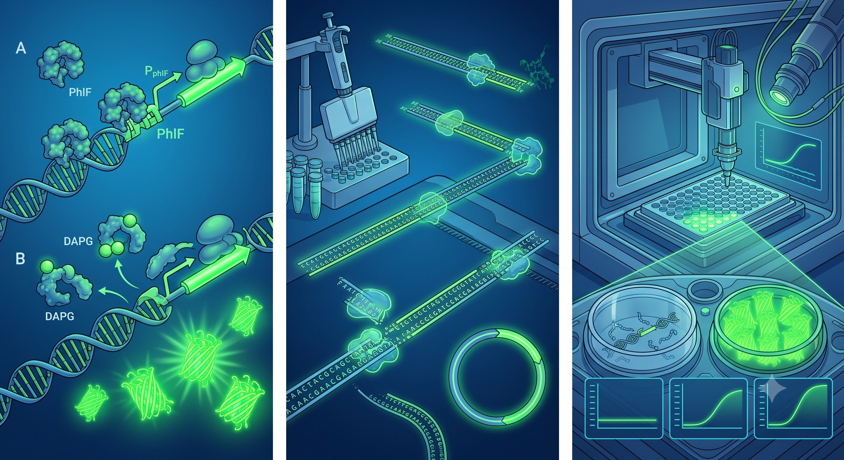
What molecule am I expressing? A protein reporter — superfolder GFP (sfGFP) — whose translation is gated by an RNA element (not itself translated) upstream of it. The thing being “sensed” is theophylline; the thing being manufactured and measured is sfGFP fluorescence as a function of theophylline concentration.

What is the sequence, and where does it come from?

• Reporter protein (sfGFP): 238 aa, derived from Aequorea victoria GFP with the point mutations S30R, Y39N, F64L, S65T, F99S, N105T, Y145F, M153T, V163A, I171V and A206V (Pédelacq et al., 2006). Canonical sequence per FPbase (GenBank ASL68970; PDB 2B3P): MSKGEELFTGVVPILVELDGDVNGHKFSVRGEGEGDATNGKLTLKFICTTGKLPVPWPTLVTTLTYGVQCFSRYPDHMKRHDFFKSAMPEGYVQERTISFKDDGTYKTRAEVKFEGDTLVNRIELKGIDFKEDGNILGHKLEYNFNSHNVYITADKQKNGIKANFKIRHNVEDGSVQLADHYQQNTPIGDGPVLLPDNHYLSTQSVLSKDPNEKRDHMVLLEFVTAAGITHGMDELYK A plasmid encoding this exact protein under a T7 promoter already exists and is orderable (Addgene plasmid #69496, “pJL1”, deposited by the Jewett lab) — I used that as my ground truth for the protein sequence rather than trusting my own recall of it.
• Sensing/regulatory element (theophylline riboswitch): the 33-nt minimal theophylline RNA aptamer originally selected by Jenison et al. (1994) by in vitro selection (SELEX) against theophylline: 5′-GGCGAUACCAGCCGAAAGGCCCUUGGCAGCGUC-3′, positioned as a translational riboswitch — fused so that, in the theophylline-free state, the aptamer’s own fold sequesters a synthetic Shine–Dalgarno/RBS sequence, and theophylline binding shifts the equilibrium to expose it for ribosome loading, following the design principle first demonstrated by Suess et al. (2004) and Desai and Gallivan (2004), and refined by Lynch et al. (2007) and Topp and Gallivan (2008). I am not inventing my own exact base-level fusion junction here — the published constructs differ in the precise spacer/overlap and get materially different ON/OFF dynamic range as a result, so the specific junction I would order is one I’d pull from a published sequence listing (or, more realistically, test 3–4 published junction variants in parallel, which is exactly the small-batch pattern HW1’s automation loop is built around) rather than guess.

What host/chassis? A cell-free (acellular) E. coli-lysate transcription–translation (TX-TL) system, consistent with HW1’s Section 2. Concretely, T7 RNA polymerase drives transcription from a T7 promoter in an E. coli S30-type extract or a reconstituted (PURE-type) system — the same cell-free format Rasor et al. (2021) argue is well suited to automation because there is no cell-viability constraint to protect. I also chose this host because a theophylline riboswitch of this exact family has already been shown to function in an E. coli S30 cell-free extract, not just in living cells (the kinetic-trapping study by the Gallivan group; Nucleic Acids Research, 2014), which is direct precedent that this mechanism survives the move out of the cell.

Where does the product need to go? Cytoplasmic — or, more precisely, free in the cell-free reaction well. No secretion or membrane targeting is needed: the read-out is fluorescence accumulation in solution, so no signal peptide or targeting tag is included.

Part 2: Genetic parts

Part 3: Assemble the construct

5′→3′ order: T7 promoter → 5′ UTR (theophylline riboswitch/RBS) → sfGFP CDS → T7 terminator, carried in the pJL1 backbone (ori + KanR). The construct map is shown above as a diagram.

Reading-frame check. I verified this computationally rather than by eye: I translated the final 717-nt CDS (see Part 4) back into protein using the standard genetic code and confirmed (a) it starts with ATG, (b) it ends with exactly one stop codon and no internal stop codons, and (c) the translated protein is character-for-character identical to the 238-aa sfGFP sequence I started from. This is the kind of check Kernel would normally run automatically on assembly; I ran it explicitly in Python to make sure my codon-optimization pass (Part 4) hadn’t silently broken the frame.

Part 4: Optimize and quality-check

Codon optimization. I wrote a short Python script and ran it (rather than describing this step abstractly) using a real E. coli K-12 codon-usage table (frequencies per 1,000 codons, sourced from GenScript’s published codon-frequency reference, itself derived from the standard Kazusa Codon Usage Database) to re-encode the sfGFP protein sequence with each amino acid’s highest-frequency E. coli codon, and compared that against a “naive” encoding of the identical protein using the equivalent human codon-usage table (from the same reference) — a realistic stand-in for what you’d get if you pulled a mammalian-optimized sfGFP sequence off the shelf without re-optimizing it for a bacterial/cell-free host.

Codon usage matters for expression in E. coli because translation rate at each codon depends on the abundance of the matching charged tRNA; codons that are rare in the host’s own genome correspond to low-abundance tRNAs, and stringing several of them together — which is exactly what happens if you keep a human-biased sequence — causes ribosome stalling, incomplete/truncated protein, and reduced overall yield. This risk is if anything sharper in a cell-free system than in vivo: a living cell can transcribe and charge more tRNA on demand, but a cell-free reaction starts with a fixed tRNA pool inherited from the lysate at preparation time and cannot replenish it, so a rare-codon bottleneck can’t be worked around mid-reaction the way it sometimes can be in vivo.

Constraint I applied, and what it caught. I did not just run the naive “pick the top codon everywhere” substitution and stop there. That first pass introduced two internal NdeI sites (CATATG) at nucleotide positions 229–234 and 649–654 — NdeI matters here specifically because it’s the actual 5′ restriction site the Jewett lab uses to clone inserts into pJL1 (confirmed directly from Addgene’s cloning-method field for several pJL1 constructs: “5′ cloning site NdeI”). Two internal NdeI sites inside the insert would let a restriction digest cut the gene itself, not just the vector boundary, which would silently wreck an NdeI/SalI cloning step. I fixed both by substituting the second-most-frequent E. coli codon (CAC instead of CAT) at the two histidine positions responsible, which removed both sites at the cost of raising the rare-codon count only slightly (from 3 to 5 of 239 codons) and leaving GC content essentially unchanged (49.1%). I also checked for SalI (GTCGAC), BsaI (GGTCTC/GAGACC) and XhoI (CTCGAG) sites (none found) and for homopolymer runs of 6+ identical bases, since long runs are a known local difficulty for both chemical synthesis and downstream sequencing (one 6-nt poly-T run remains in the optimized sequence — noted as a mild synthesis-difficulty flag in Part 5, not something I removed, since doing so would mean drifting further from the optimal codon at that position for a single-nucleotide-run issue most vendors handle routinely).

Final, NdeI/SalI-clean, E. coli-codon-optimized sfGFP CDS (717 nt, verified to translate back to the exact original protein with no internal stops):

ATGAGCAAAGGCGAAGAACTGTTTACCGGCGTGGTGCCGATTCTGGTGGAACTGGATGGCGATGTGAACGGCCATAAATTTAGCGTGCGTGGCGAAGGCGAAGGCGATGCGACCAACGGCAAACTGACCCTGAAATTTATTTGCACCACCGGCAAACTGCCGGTGCCGTGGCCGACCCTGGTGACCACCCTGACCTATGGCGTGCAGTGCTTTAGCCGTTATCCGGATCACATGAAACGTCATGATTTTTTTAAAAGCGCGATGCCGGAAGGCTATGTGCAGGAACGTACCATTAGCTTTAAAGATGATGGCACCTATAAAACCCGTGCGGAAGTGAAATTTGAAGGCGATACCCTGGTGAACCGTATTGAACTGAAAGGCATTGATTTTAAAGAAGATGGCAACATTCTGGGCCATAAACTGGAATATAACTTTAACAGCCATAACGTGTATATTACCGCGGATAAACAGAAAAACGGCATTAAAGCGAACTTTAAAATTCGTCATAACGTGGAAGATGGCAGCGTGCAGCTGGCGGATCATTATCAGCAGAACACCCCGATTGGCGATGGCCCGGTGCTGCTGCCGGATAACCATTATCTGAGCACCCAGAGCGTGCTGAGCAAAGATCCGAACGAAAAACGTGATCACATGGTGCTGCTGGAATTTGTGACCGCGGCGGGCATTACCCATGGCATGGATGAACTGTATAAATAA

Sequence search (in place of a Kernel/BLAST run). I don’t have BLAST access via Kernel right now, and I’d rather say that plainly than fabricate a BLAST report, so here is the honest, reasoned version of the same question. Because I built this CDS by reverse-translating a reference protein sequence rather than by editing an existing deposited DNA sequence, I can say with certainty, by construction, what a real search would find: at the protein level, a tblastn-style search would return a very close (likely 100%, modulo the exact GFP numbering convention used) match to the original superfolder GFP sequence from Pédelacq et al. (2006) — this is a well-known, extensively re-derived engineered protein, not a natural gene and not novel. At the nucleotide level, a blastn-style search would not return 100% identity to any single deposited plasmid sequence (including the original pJL1-sfGFP), because I chose fresh, optimized codons at roughly half of all 239 positions — those substitutions are synonymous (silent at the protein level) but real at the DNA level. So the honest answer to “is it identical to a natural gene, or novel?” is: the protein is an established, non-natural, previously engineered variant with a well-known closest match; the specific codon-level DNA sequence I designed is a fresh (if unremarkable) synonymous variant of an existing construct, not identical to any one deposited record. I would confirm this with an actual BLAST/Kernel search before ordering.

Safety screen (reasoned, not run). Commercial and academic DNA synthesis screening today generally follows either the International Gene Synthesis Consortium’s Harmonized Screening Protocol or the equivalent US HHS Screening Framework Guidance (issued 2010, updated 2023), and a growing share of providers additionally run IBBIS’s open-source Common Mechanism tool, which uses sequence-alignment methods (BLAST, DIAMOND, HMMER, cmscan) against curated databases of regulated/hazardous (“sequences of concern”) biological sequences as well as general NCBI databases, on a minimum 50-nt screening window (Wheeler et al., 2024). I would expect this construct to come back clean, and I can say why rather than just asserting it: none of the four parts derive from a regulated pathogen, toxin, or select agent — sfGFP derives from a non-pathogenic jellyfish (Aequorea victoria); the theophylline aptamer is a fully synthetic, in-vitro-selected sequence with no natural viral, bacterial, or toxin origin; the T7 promoter/terminator derive from bacteriophage T7, which is not itself a regulated pathogen; and the pJL1 backbone’s KanR marker and pUC-derived origin are standard, widely-distributed cloning-vector elements. If a screen did flag something here, given the specific parts involved, I’d expect it to be a low-confidence, short-window coincidental match rather than a genuine hazard, and I’d want to see exactly which database hit fired before assuming it’s a false positive.

Part 5: From design to build

How would I build it? The full insert I need synthesized — T7 promoter through T7 terminator — is roughly 850 bp (promoter ~20 bp + riboswitch/RBS 5′ UTR ~60–100 bp + 717-bp sfGFP CDS + terminator ~50 bp), well within the length a commercial vendor synthesizes as a single linear double-stranded DNA fragment (a “gene fragment”/gBlock-class product) rather than something that needs to be built up from smaller pieces by hand. I would order that fragment directly and clone it into a linearized pJL1 backbone by Gibson assembly — not a guess: Gibson assembly (Gibson et al., 2009) is the literal cloning method Addgene’s own records list for several existing pJL1-family constructs (including the sfGFP-expressing ones), which tells me this exact backbone-plus-insert combination is routinely built this way in practice. Gibson assembly is a good fit here specifically because it’s a single-tube, sequence-homology-based reaction that doesn’t depend on convenient restriction sites — relevant given that my codon optimization pass in Part 4 had to actively remove restriction sites the naive optimization introduced, which is exactly the kind of constraint Gibson assembly sidesteps for the vector-insert junction (even though the pJL1-internal NdeI/SalI sites still mattered for my codon choice inside the CDS itself, since some constructs in this same lineage are built by restriction cloning instead).

What does synthesis constrain, and does my design have anything hard to synthesize? Chemical (phosphoramidite) DNA synthesis has a per-coupling error rate that compounds with length and is worse in regions with strong secondary structure, high GC content, or repetitive/homopolymeric runs, which is why gene-length constructs historically needed post-synthesis error correction — Carr et al. (2004) describe an enzymatic approach using the mismatch-binding protein MutS to selectively cleave and remove error-containing duplexes from a synthesis pool, which is the direct ancestor of the sequencing-verification step every modern commercial gene-synthesis vendor now runs by default. My design has two features worth flagging under this lens, both of which I found computationally rather than by inspection: (1) the E. coli-optimized CDS still contains one six-nucleotide poly-T run, a known locally error-prone motif for synthesis and sequencing; and (2) the riboswitch element is, by design, a folded RNA structure (that’s the entire mechanism — it has to fold to sequester the RBS) — the corresponding DNA template will have real secondary-structure-forming potential in that region, which can stall polymerase during both chemical synthesis and any PCR-based amplification step, exactly the class of problem Carr et al. (2004) and the chip-based synthesis literature discuss.

Prototype vs. scale. For this single validation construct, ordering one synthesized fragment plus one Gibson assembly reaction is the right scale of tool — anything more elaborate would be solving a problem I don’t have yet. But this construct is explicitly a stand-in for what HW1’s automation loop will eventually need to build many of: candidate riboswitch/RBS-junction variants (and, later, entirely new aptamer sequences) tested in parallel batches. At that scale, ordering each variant as an individually synthesized fragment stops being the right tool — this is exactly the problem chip-based, multiplexed oligo synthesis was built to solve. Tian et al. (2004) and Kong et al. (2007) demonstrate parallel gene synthesis directly on programmable DNA microchips, and Kosuri et al. (2010) show how to go from a chip-synthesized oligo pool to selectively amplified, gene-length constructs at far lower per-sequence cost than individually ordered oligos. This directly answers a gap I flagged but couldn’t source in HW1’s Section 4a, where I estimated the design-phase campaign’s oligo cost using individually-ordered-oligo pricing and only speculated, without a citation, that pooled/array synthesis would be “one to two orders of magnitude” cheaper for exactly this kind of large combinatorial library — Kosuri et al. (2010) is the citation that claim needed.

Part 6: What don’t you know yet

1. Whether the riboswitch retains its reported dynamic range in this exact pairing. The theophylline-riboswitch mechanism is confirmed to work in living E. coli cells (Desai and Gallivan, 2004; Topp and Gallivan, 2008) and, separately, in E. coli S30 cell-free extract in general (the 2014 Nucleic Acids Research kinetic-trapping study from the Gallivan group) — but not, as far as I found, with this specific riboswitch fused directly to sfGFP in the pJL1/T7 architecture. I would find this out with a straightforward with/without-theophylline fluorescence titration in the actual cell-free reaction, across a concentration range bracketing the reported theophylline aptamer binding Kd (~400 nM in vitro) and the much higher concentration (~300–500 µM) historically needed to activate these riboswitches in intact cells.

2. Whether the exact aptamer-to-RBS junction I have not yet committed to matters as much as the literature suggests it does. I deliberately did not invent a specific base-level fusion sequence in Part 1/2 because published variants of this riboswitch family differ in spacer length and overlap and get materially different ON/OFF ratios as a result. I would want to build and test a small panel of 3–4 published junction variants side by side rather than commit the whole downstream cloning effort to just one on the first pass — which is, not coincidentally, exactly the small parallel-batch pattern HW1’s automated lab-in-the-loop system is designed to run.

3. Whether my codon-optimization changes altered local mRNA structure near the start codon in a way that matters. I checked reading frame, restriction sites, GC content and rare-codon burden computationally, but I did not model the folding energy of the actual designed 5′ region (riboswitch + start codon + first several CDS codons), and translation-initiation rate in bacteria is known to be sensitive to secondary structure right around the ribosome binding site — a change that’s silent at the protein level can still change how fast ribosomes load. I would check this with an RNA-folding tool (e.g. RNAfold) on the final designed sequence before ordering, which is exactly the kind of check I’d expect Kernel to surface automatically once I have access to it.

AI use disclosure

I used the Claude Sonnet 5 model accessed via claude.ai, as a research and drafting assistant for this assignment, continuing directly from the same conversation and AI-assisted workflow described in my Homework #1 submission.

References

Bu, Y., Liu, Y., Hu, A., Lee, Y.C. and Yobas, L. (2026) ‘Auto-SELEX: a fully automated microfluidic platform for rapid discovery of high-affinity aptamers’, Lab on a Chip, 26(14), pp. 4117–. https://doi.org/10.1039/D6LC00275G

Carr, P.A., Park, J.S., Lee, Y.-J., Yu, T., Zhang, S. and Jacobson, J.M. (2004) ‘Protein-mediated error correction for de novo DNA synthesis’, Nucleic Acids Research, 32(20), e162. https://doi.org/10.1093/nar/gnh160

Desai, S.K. and Gallivan, J.P. (2004) ‘Genetic screens and selections for small molecules based on a synthetic riboswitch that activates protein translation’, Journal of the American Chemical Society, 126(41), pp. 13247–13254. https://doi.org/10.1021/ja048634j

Elowitz, M.B. and Leibler, S. (2000) ‘A synthetic oscillatory network of transcriptional regulators’, Nature, 403, pp. 335–338. https://doi.org/10.1038/35002125

GenScript (n.d.) Codon usage frequency table. Available at: https://www.genscript.com/tools/codon-frequency-table (Accessed: 29 September 2026). Note: technical/vendor reference table (Kazusa Codon Usage Database-derived), not a peer-reviewed source; used here only as the source of the raw per-codon frequency figures I computed with.

Gibson, D.G., Young, L., Chuang, R.-Y., Venter, J.C., Hutchison, C.A. and Smith, H.O. (2009) ‘Enzymatic assembly of DNA molecules up to several hundred kilobases’, Nature Methods, 6, pp. 343–345. https://doi.org/10.1038/nmeth.1318

Jenison, R.D., Gill, S.C., Pardi, A. and Polisky, B. (1994) ‘High-resolution molecular discrimination by RNA’, Science, 263(5152), pp. 1425–1429. https://doi.org/10.1126/science.7510417

Kong, D.S., Carr, P.A., Chen, L., Zhang, S. and Jacobson, J.M. (2007) ‘Parallel gene synthesis in a microfluidic device’, Nucleic Acids Research, 35(8), e61. https://doi.org/10.1093/nar/gkm121

Kosuri, S., Eroshenko, N., LeProust, E.M., Super, M., Way, J., Li, J.B. and Church, G.M. (2010) ‘Scalable gene synthesis by selective amplification of DNA pools from high-fidelity microchips’, Nature Biotechnology, 28, pp. 1295–1299. https://doi.org/10.1038/nbt.1716

Lambert, T.J. (2019) ‘FPbase: a community-editable fluorescent protein database’, Nature Methods, 16, pp. 277–278. https://doi.org/10.1038/s41592-019-0352-8

Lynch, S.A., Desai, S.K., Sajja, H.K. and Gallivan, J.P. (2007) ‘A high-throughput screen for synthetic riboswitches reveals mechanistic insights into their function’, Chemistry & Biology, 14(2), pp. 173–184. https://doi.org/10.1016/j.chembiol.2006.12.008

Martin, R.W., Des Soye, B.J., Kwon, Y.-C., Kay, J., Davis, R.G., Thomas, P.M., Majewska, N.I., Chen, C.X., Marcum, R.D., Weiss, M.G., Stoddart, A.E., Amiram, M., Ranji Charna, A.K., Patel, J.R., Isaacs, F.J., Kelleher, N.L., Hong, S.H. and Jewett, M.C. (2018) ‘Cell-free protein synthesis from genomically recoded bacteria enables multisite incorporation of noncanonical amino acids’, Nature Communications, 9, 1203. https://doi.org/10.1038/s41467-018-03469-5

Pédelacq, J.-D., Cabantous, S., Tran, T., Terwilliger, T.C. and Waldo, G.S. (2006) ‘Engineering and characterization of a superfolder green fluorescent protein’, Nature Biotechnology, 24(1), pp. 79–88. https://doi.org/10.1038/nbt1172

Rasor, B.J., Vögeli, B., Landwehr, G.M., Bogart, J.W., Karim, A.S. and Jewett, M.C. (2021) ‘Toward sustainable, cell-free biomanufacturing’, Current Opinion in Biotechnology, 69, pp. 136–144. https://doi.org/10.1016/j.copbio.2020.12.012

Stanton, B.C., Nielsen, A.A.K., Tamsir, A., Clancy, K., Peterson, T. and Voigt, C.A. (2014) ‘Genomic mining of prokaryotic repressors for orthogonal logic gates’, Nature Chemical Biology, 10, pp. 99–105. https://doi.org/10.1038/nchembio.1411

Tian, J., Gong, H., Sheng, N., Zhou, X., Gulari, E., Gao, X. and Church, G. (2004) ‘Accurate multiplex gene synthesis from programmable DNA microchips’, Nature, 432, pp. 1050–1054. https://doi.org/10.1038/nature03151

Topp, S. and Gallivan, J.P. (2008) ‘Riboswitches in unexpected places — a synthetic riboswitch in a protein coding region’, RNA, 14(12), pp. 2498–2503. https://doi.org/10.1261/rna.1225108

Wachsmuth, M., Domin, G., Lorenz, R., Serfling, R., Findeiß, S., Stadler, P.F. and Morl, M. (2014) ‘A family of synthetic riboswitches adopts a kinetic trapping mechanism’, Nucleic Acids Research, 42(10), pp. 6753–6761. https://doi.org/10.1093/nar/gku262

Wheeler, N.E. et al. (2024) ‘Developing a common global baseline for nucleic acid synthesis screening’, Applied Biosafety, 29(2), pp. 71–78. https://doi.org/10.1089/apb.2023.0034

Week 3 HW: Cell-Free Protocols

HTBAA Homework #3: Designing a Cell-Free Reaction Composition

Prepared by: Nitin Due: Tuesday, 6 October 2026

0. Scope, and how this relates to my main project

This is a deliberate branch off my HW1/HW2 thread rather than a continuation of it. My main project is a lab-in-the-loop system for discovering aptamer biosensors, and in HW2 I designed a theophylline-riboswitch-gated sfGFP construct to validate the cell-free layer of that pipeline. HW3 fixes the three protein targets (sfGFP, PETase, Reteplase) and fixes the reporter sequence, so the riboswitch design does not transfer directly. What does transfer is the reaction chemistry underneath it: every assay in my pipeline runs in an E. coli lysate CFPS reaction, so a cheaper and more reproducible reaction composition lowers the per-assay cost of my entire HW1 scale estimate. I return to that connection briefly in Section D.

One scoping note on provenance: I could not access coopetition.htgaa.org, which requires an HTGAA Keycloak login. That means I do not have the actual reagent menu, the available stock concentrations, or the current community reagent list. Every volume in Section B is therefore computed against assumed stock concentrations and must be recomputed against the real menu before submission. I have flagged this at the point of use rather than burying it here.

A sequence check worth doing first

I verified the three supplied sequences rather than taking the handout’s stated sizes at face value, because $/g is inversely proportional to molecular weight and a tag changes it:

The cysteine counts confirm the handout’s folding-difficulty argument exactly (0, 1 and 9 disulfide bonds). The length and mass discrepancies for PETase and Reteplase are not errors: the supplied constructs carry N-terminal Strep-tag II (WSHPQFEK) plus a TEV site (ENLYFQ) and linkers, and sfGFP carries a C-terminal Strep-tag II. The handout’s figures describe the untagged mature proteins. This matters for the coopetition objective: if titer is quantified on the tagged construct, the $/g denominator should use the tagged mass (33.2 and 44.1 kDa), which is roughly 13–19% higher than the untagged values and therefore makes $/g look correspondingly better. Worth confirming which convention the scoring uses.

A. Compare cell-free reaction compositions

A1. Why potassium glutamate and magnesium glutamate concentrations differ, and which is more sensitive

The two differ by more than an order of magnitude in every published formulation — potassium glutamate sits at roughly 130–200 mM while magnesium glutamate sits at roughly 4–12 mM — because they do different jobs.

Potassium glutamate sets bulk ionic strength and is there to mimic the E. coli cytoplasm, which is the explicit founding premise of PANOx-SP (Jewett and Swartz, 2004). Glutamate is deliberately chosen as the counter-ion over acetate or chloride because glutamate is the dominant cytoplasmic anion. Its optimum is broad: it is a bulk electrostatic environment, not a stoichiometric participant.

Magnesium glutamate is a catalytic and structural cofactor. Mg²⁺ mediates ribosomal subunit association, stabilises tRNA and mRNA tertiary folds, and is stoichiometrically complexed with nucleotide triphosphates (the true polymerase substrate is Mg-ATP, not free ATP). Too little and ribosomes dissociate and polymerases stall; too much and translational fidelity drops and nucleotides are over-chelated. Its optimum is correspondingly narrow.

Magnesium is clearly the more sensitive of the two, and I want to ground that in experimental behaviour rather than assert it mechanistically. The strongest evidence is what the Olsen et al. (2026) team actually re-optimised: they re-determined magnesium and phosphate concentrations for every new lysate batch, for every change in lysate concentration, and for every new source strain — and did not do the same for potassium glutamate. A parameter that must be retuned per lysate batch is, by definition, the sensitive one. Two further observations support this: E. coli extract optima cluster tightly at 8–12 mM Mg(Glu)₂, whereas a C. autoethanogenum extract optimised at 32 mM with a reported five-orders-of-magnitude swing in luciferase expression across the 8–36 mM range (Krüger et al., 2020) — an enormous response to a modest concentration change; and across the eight formulations Olsen et al. tabulated, magnesium glutamate barely moves (4–12 mM) precisely because it has so little room to move.

Practical consequence for the coopetition: magnesium is the parameter most likely to cause a composition that wins in round 1 to fail reproducibility in round 2, because the 96-well re-test may use a different lysate batch. Spending screening budget on a magnesium titration around the chosen point is better insurance than optimising a dozen cheap salts.

A2. PEP+NTP versus ribose+NMP formulations

These are two different answers to the same question: where does the ATP come from?

PEP + NTP (the PANOx-SP approach). Nucleotides are supplied directly as triphosphates (ATP ~1.2 mM; GTP/UTP/CTP ~0.86 mM each), and phosphoenolpyruvate at ~33 mM acts as a high-energy secondary phosphate donor, regenerating ATP from ADP via pyruvate kinase. It works well and was the highest-yielding formulation in Olsen et al.’s own head-to-head comparison. It has two problems. Cost: PEP alone runs roughly $2,000–3,000 per litre of reaction, pushing total reagent costs above $4,000/L and accounting for over 75% of material costs. Metabolic dynamics: Olsen et al. measured the time course directly and found ATP surges within 30 minutes and then falls to nearly zero, while inorganic phosphate rises sharply and stays high because Pi is liberated stoichiometrically as PEP is consumed. Accumulated phosphate chelates magnesium and the reaction dies early — the system is energetically front-loaded and short-lived.

Ribose + NMP (the RF_opt approach). Nucleotides are supplied as monophosphates, which are far cheaper, and the lysate’s own surviving kinase activity phosphorylates them up to triphosphates in situ. Energy comes from non-phosphorylated carbon sources — ribose, maltodextrin, glucose — feeding glycolysis to regenerate ATP. The measured behaviour is qualitatively different: RF_opt begins with no exogenous ATP at all, yet reaches comparable ATP within 30 minutes and then sustains roughly 250 µM for the entire reaction, well above the ATP affinity threshold for cell-free expression. Phosphate stays at 10–15 mM, about three-fold lower than PANOx-SP. The outcome is a longer-lived reaction: 2.4 ± 0.3 g/L sfGFP, an 87% yield increase over PANOx-SP, at 99% lower reagent cost.

Two constraints and one caveat that matter for design. NMP concentrations must be capped at about 5 mM or insoluble precipitates form, and NMPs must be added to the reagent mix last. Separately, Olsen et al. found GMP can be replaced by guanine plus ribose with no yield penalty — relevant to Section C below. The caveat: RF_opt buys its cost advantage at the price of robustness. It is more sensitive to lysate amount than PANOx-SP, more sensitive to surface-area-to-volume ratio (because it is oxygen-limited), and needs per-lysate magnesium and phosphate retuning. In a 384-well plate at 20 µL — a high surface-area-to-volume, oxygen-rich geometry — that sensitivity may actually work in our favour, but it is the main reason a cheap composition can fail to reproduce on scale-up to 2 mL tubes.

A3. Compare and contrast two published formulations: PANOx-SP versus RF_opt

What the comparison actually teaches. The headline is not “fewer components” but that removing expensive components and switching the energy strategy raised yield. Olsen et al. explored 1,231 reaction mixtures to get there, and a minimal formulation of only potassium glutamate, NMPs and amino acids was already productive at 0.5 g/L. That is the single most useful prior for this coopetition: the design space rewards subtraction, and reagents that feel obligatory (tRNA, CoA, NAD⁺) are dispensable when the lysate is not dialysed. It also reframes the cost problem — in RF_opt, reagents fall from 75% of total material cost to under 4%, meaning that once you adopt a cheap formulation, lysate and DNA dominate and further reagent trimming has sharply diminishing returns.

Provenance warning on the cost figures

These numbers are widely quoted in mutually incompatible ways, and I think this is worth stating explicitly before anyone builds a cost model on them.

• Olsen et al. is peer-reviewed (Nature Communications, 5 March 2026, 17:3478). The published version reports ~$60/g_protein at the 15 µL scale and ~$39/g at 4 mL with oxygen supplementation. The August 2025 bioRxiv preprint of the same work reports $55/g and $36/g. The figures shifted between preprint and publication; the published values should be cited.
• Smith et al. (2026) is a preprint (bioRxiv, 5 February 2026) and has not been peer reviewed. It reports sfGFP at $422/g versus what it calls Olsen et al.’s $698/g — a 40% improvement, with a 27% titer increase, from six rounds and roughly 29,000–36,000 conditions on Ginkgo’s RAC cloud lab.
• These two sets of numbers are not comparable. Olsen’s ~$60/g counts reagents only; Smith’s $422/g counts total reaction components including lysate and DNA. Quoting “$60/g” and “$422/g” in the same table as though they measure the same thing would be wrong by roughly an order of magnitude. Note also that the 36,000-experiment figure comes from Ginkgo’s own press release, not the preprint’s abstract, and press-release figures should be labelled as such.

My own sanity check, flagged as inference rather than a sourced result. Lysate is fixed at 5,000 nL per 20 µL reaction, so at $4.00/mL it contributes exactly $0.02 per reaction regardless of composition. At a 2.4 g/L titer, a 20 µL reaction yields 48 µg, so lysate alone sets a floor of about $417/g. That this lands within 1% of Smith et al.’s reported $422/g total is striking and suggests their number is almost entirely lysate-dominated at a titer near 2.4 g/L. I have not verified their titer or cost basis, so treat this as a hypothesis to check against their Table 1 — but if it holds, it means the only lever that materially moves $/g in this coopetition is titer, not reagent cost. Reagent trimming below a certain point is optimising a rounding error.

For orientation, the lysate-only floor at other titers:

B. Three reaction compositions

Read this before the tables. Volumes are computed as V = 20,000 nL × C_final / C_stock, rounded to the nearest 25 nL as the specification requires. The stock concentrations are my assumptions, since I could not reach the coopetition reagent menu. The target final concentrations are the real design content and are grounded in the citations given; the nanolitre volumes are arithmetic that must be recomputed against the actual menu stocks. Rounding to 25 nL introduces up to roughly 6% error on the smallest additions (spermidine, putrescine), which is acceptable for those but would not be for magnesium — if the real stock makes magnesium land awkwardly, dilute the stock rather than accept the rounding error, for the sensitivity reasons in A1.

All three designs follow the RF_opt direction (NMP + non-phosphorylated energy, no PEP, no tRNA/CoA/NAD⁺), because A3 establishes that this is both cheaper and higher-yielding, and because A’s cost analysis says titer is what matters.

Design 1 — sfGFP (reducing)

Rationale: an RF_opt-direction composition using the 5 mM NMP cap, maltodextrin and ribose for ATP regeneration, spermidine retained (both Olsen et al. and Smith et al. identify spermidine as yield-positive), and no PEP, tRNA, CoA or NAD⁺. The 1,400 nL of headroom is deliberate: it is the room to run a magnesium titration (A1) without rebuilding the whole composition.

Design 2 — PETase (reducing)

I would submit the Design 1 composition unchanged for PETase in round 1. This is an experimental-design choice, not laziness, and I want to defend it explicitly. TfCut2 has one disulfide bond and the handout states it remains compatible with reducing conditions, so there is no mechanistic reason to switch regimes. More importantly, I have no PETase-specific data, and the handout’s own framing — that a composition performing well for one protein may perform poorly for another — is a hypothesis that only gets tested if someone submits the same composition across two proteins. Submitting an sfGFP-optimal composition for PETase measures the transfer gap directly and tells the community something the all-variants-differ approach cannot. If the transfer gap turns out to be large, round 2 has a clear direction: a lower magnesium variant, since the longer transcript and the single disulfide may shift the optimum.

Design 3 — Reteplase (oxidising / DSB)

Also specified outside the variable budget: BL21 Star (DE3) Δgor lysate, IAM-treated at the low dose (25 µM, not 500 µM), with the IAM quenched by cysteine.

The design decision that matters here, and why. The handout tells you Reteplase needs GSSG/GSH and DsbC. What it does not tell you is that bolting that oxidising module onto a low-cost non-phosphorylated formulation is actively dangerous. Olsen et al. found that adding IAM, GSSG and GSH to RF_opt reduced sfGFP production by 75–97%. They traced the mechanism: glutathione addition drops the reaction pH, and because RF_opt is already more acidic than PANOx-SP, the pH falls below 7.0 — outside the 7.4–7.8 cytoplasmic range where PANOx-SP comfortably sits. Two fixes recovered the yield: raising the HEPES buffer to pH 7.5, and knocking out glutathione reductase (Δgor) in the lysate source strain, which let them use 20-fold less IAM (25 µM rather than 500 µM) while stabilising the oxidising environment. Both are built into the design above. Without the pH 7.5 specification, I would expect this composition to fail badly, and I think that is the most likely silent failure mode for anyone submitting a cheap oxidising Reteplase formulation.

The specific values — 4 mM GSSG, 1 mM GSH (a 4:1 oxidised:reduced ratio), 5 µM purified DsbC, 25 µM IAM, Δgor — are Olsen et al.’s, not invented. There is also a direct functional precedent: they expressed vtPA, a truncated tissue plasminogen activator closely related to Reteplase, in oxidised RF_opt and showed it was enzymatically active using the IPR-AMC fluorogenic assay — the same substrate and the same assay the handout specifies for Reteplase here. That is about as close to a validated starting point as this target has. Note, though, that even with the pH fix, glutathione addition still reduced yields by up to 62% in their hands, so Reteplase should be expected to be the lowest-titer and highest-$/g of the three targets regardless of composition.

C. Community reagent proposal: guanine

Proposal: add guanine (the free nucleobase) to the reagent inventory.

How I decided on it. I worked backwards from where the remaining cost actually sits. Section A establishes that once PEP is removed, NMPs become the most expensive reagent group in the minimal formulation — Olsen et al. put them at $62/g_protein — and that lysate then dominates everything else. So the only reagent-side lever left with real headroom is making nucleotides cheaper. Olsen et al. tested exactly this and report a specific, actionable result: most individual replacements of nucleoside monophosphates with their corresponding nucleosides or nucleobases decreased yield, but GMP could be replaced by a combination of guanine and ribose with no loss of protein yield. They name this in their discussion as “one potential path” to lower cost. Ribose is already on the menu under energy regeneration; guanine, as far as I can tell from the handout’s category table, is not. So the single missing piece needed to test a published, yield-neutral cost reduction is one cheap nucleobase.

Why it is a good coopetition reagent specifically: it is a targeted substitution with a published positive result behind it rather than a speculative addition, it attacks the largest remaining reagent cost, nucleobases are substantially cheaper than nucleotides, and it is a clean single-variable experiment (swap GMP for guanine, hold everything else) that fits the staged screening design well. If it works, adenine, cytosine and uracil are the obvious follow-ups — though Olsen et al.’s data suggests those will not transfer, since guanine was the surprising exception rather than the rule. That asymmetry is itself worth knowing.

Caveat I would post with it: Olsen et al. observed insoluble precipitates with many nucleotide alternatives and explicitly flagged precipitate formation as needing further investigation. Guanine has poor aqueous solubility at neutral pH, so this needs a solubility check at the intended stock concentration before it goes into an Echo acoustic dispenser — nanolitre acoustic transfer is unforgiving of precipitates, and a reagent that crashes out in the source plate will silently wreck a whole 384-well run.

A second idea for the forum (more speculative, and I would label it as such). Olsen et al. found dissolved oxygen was the largest single lever they identified — switching from a 20% to a 100% O₂ feed raised sfGFP from under 2 g/L to 3.7 ± 0.2 g/L, a 45% improvement, and they note RF_opt-style formulations are especially sensitive to surface-area-to-volume ratio. The menu already carries catalase and pyruvate oxidase under oxygen-related components. Whether an oxygen-carrier additive would help in a sealed 384-well plate is a reasonable question, but I have not found a CFPS paper testing one, so I would raise it as a question rather than a recommendation.

D. Connection back to the main project

Three things from this homework feed my HW1 pipeline.

The cost model changes. My HW1 estimate costed the design phase on oligonucleotide synthesis and treated the assay as negligible. The arithmetic in Section A says the assay floor is set by lysate and titer, not reagents — roughly $417/g at a 2.4 g/L titer. For a pipeline running thousands of 20 µL reporter assays, that is the number to plan around, and it is a correction to HW1.

The coopetition is a working instance of my proposed loop. Smith et al. is GPT-5 proposing compositions, a cloud lab executing them, and results returning to the model over six rounds — structurally the same closed loop I proposed in HW1, with a Pydantic schema doing the design-to-protocol validation step I described abstractly. Their reported sub-1% error rate for AI-designed plates reaching the lab is a useful benchmark for the protocol-generation step I hand-waved.

One hypothesis I now want to test. A composition optimised for maximum sfGFP titer is not necessarily optimal for a riboswitch biosensor, which needs low background and high dynamic range rather than maximum absolute signal. Magnesium is the obvious suspect, since Section A1 establishes it as the sensitive parameter and Mg²⁺ also stabilises RNA tertiary structure — the very folding the riboswitch depends on. I flagged this intuition in discussion before doing the reading and could not source it then; I still cannot source it for riboswitches specifically, so it remains my hypothesis. But it is now a sharper and more testable one: titrate magnesium against ON/OFF ratio rather than against titer, and expect the two optima to diverge.

E. What I do not know

1. The actual reagent menu and stock concentrations. Every nanolitre figure in Section B is provisional until recomputed against coopetition.htgaa.org. The target concentrations are the defensible part.
2. RF_opt’s complete component list. I have its character — 12 components, NMP-based, maltodextrin and ribose, HEPES, spermidine, no tRNA/CoA/NAD⁺ — and several exact values, but not the full Table 1 with every concentration. My Design 1 is RF_opt-directional, built on PANOx-SP’s well-documented salt concentrations with RF_opt’s energy strategy substituted in. Pulling the real Table 1 would improve it.
3. Whether my lysate-floor inference is right. The $417/g versus $422/g coincidence is suggestive, not established. It needs checking against Smith et al.’s Table 1 before anyone relies on the conclusion that titer is the only lever that matters.

AI use disclosure

I used Claude (Anthropic, Claude Opus 5 as a research and drafting assistant for this assignment, continuing directly from the same conversation and AI-assisted workflow described in earlier HW.

References

Jewett, M.C. and Swartz, J.R. (2004) ‘Mimicking the Escherichia coli cytoplasmic environment activates long-lived and efficient cell-free protein synthesis’, Biotechnology and Bioengineering, 86(1), pp. 19–26. https://doi.org/10.1002/bit.20026

Krüger, A., Mueller, A.P., Rybnicky, G.A., Engle, N.L., Yang, Z.K., Tschaplinski, T.J., Simpson, S.D., Köpke, M. and Jewett, M.C. (2020) ‘Development of a clostridia-based cell-free system for prototyping genetic parts and metabolic pathways’, Metabolic Engineering, 62, pp. 95–105. https://doi.org/10.1016/j.ymben.2020.06.004

Olsen, M.L., Copeland, C.E., Sundberg, C.A., Aw, R., Shaver, Z.M., Rao, G., Swartz, J.R., Karim, A.S. and Jewett, M.C. (2026) ‘Design-driven optimization of low-cost reagent formulations for reproducible and high-yielding cell-free gene expression’, Nature Communications, 17(1), 3478. https://doi.org/10.1038/s41467-026-69605-8 (Peer-reviewed. Preprint version: bioRxiv, https://doi.org/10.1101/2025.08.01.668204, August 2025 — cost figures differ slightly between the two; published values cited here.)

Rasor, B.J., Vögeli, B., Landwehr, G.M., Bogart, J.W., Karim, A.S. and Jewett, M.C. (2021) ‘Toward sustainable, cell-free biomanufacturing’, Current Opinion in Biotechnology, 69, pp. 136–144. https://doi.org/10.1016/j.copbio.2020.12.012

Silverman, A.D., Karim, A.S. and Jewett, M.C. (2020) ‘Cell-free gene expression: an expanded repertoire of applications’, Nature Reviews Genetics, 21, pp. 151–170. https://doi.org/10.1038/s41576-019-0186-3

Smith, A.A., Wong, E.L., Donovan, R.C., Chapman, B.A., Harry, R., Tirandazi, P., Kanigowska, P., Gendreau, E.A., Dahl, R.H., Jastrzebski, M., Cortez, J.E., Bremner, C.J., Che, J.C., Thavarajah, W., Smith, D. and Thomas, T.F. (2026) ‘Using a GPT-5-driven autonomous lab to optimize the cost and titer of cell-free protein synthesis’, bioRxiv [preprint], 5 February. https://doi.org/10.64898/2026.02.05.703998 (Not peer-reviewed. The 36,000-condition figure comes from Ginkgo Bioworks’ accompanying press release, not the preprint abstract.)

Final Project